Abstract
3D sound propagation modeling in the context of acoustic noise monitoring problems is considered. A technique of effective source spectrum reconstruction from a reference single-hydrophone measurement is discussed, and the procedure of simulation of sound exposure level (SEL) distribution over a large sea area is described. The proposed technique is also used for the modeling of pulse signal waveforms at other receiver locations, and results of a direct comparison with the pulses observed in the experimental data is presented.
1. Introduction
Monitoring of acoustic energy levels distribution over a large sea areas due to anthropogenic noises generated in course of various industrial activities on the continental shelf is one of applications for which 3D sound propagation models are necessary [1,2,3,4,5,6,7]. Indeed, it is absolutely impossible to cover the entire sea area of interest by receivers, and few point-wise reference measurements should be used to reconstruct the soundscape of the marine environment. It is often desirable to conduct comprehensive monitoring of noise pollution of the sea area in real time in order to provide a possibility for prompt assessment of its impact on the marine fauna and for undertaking adequate noise mitigation measures in a timely manner [1]. This challenge imposes severe restrictions on the performance of computational codes for sound propagation modelling. For example, in the case of acoustical monitoring of seismic survey a problem of simulating broadband (10–250 Hz) pulses propagation in 3D computational domain representing a sea area that stretches for tens of kilometers in both horizontal directions [3,8]. Many existing techniques for the modeling of sound propagation cannot meet the requirement that broadband simulation in such domain must be carried out almost in real time. For example, it is known that within the framework of modern highly-accurate approach based on 3D parabolic equation (PE) it takes about 20 h to compute acoustic field at one single frequency of 25 Hz in the wedge benchmark problem [9]. Thus, one can hardly rely on 3D PEs for performing simulation of broadband sources in a timely manner.
A good compromise between the accuracy of the field modeling and efficiency of computations can be achieved by using the mode parabolic equations (MPE) theory [10,11,12,13]. During the past decade several computational models based on this approach were developed at POI. Among them there is a code based on narrow-angle MPE with mode coupling taken into account [14], as well as the code based on the adiabatic wide-angle and pseudodifferential MPEs [12,15].
In this study we discuss practical applications of MPE-based methods of acoustic field computations to the problems of the modeling of sound exposure levels [8] (SEL) distributions arising when performing monitoring of seismic survey in a given sea area. The estimation of SEL distribution consists in a three-step procedure:
- 1
- the reconstruction of effective spectrum of a point source approximating a set of airguns from a point-wise reference measurement data obtained using an autonomous underwater acoustic recorder;
- 2
- the multi-frequency simulation of acoustic field in the area of interest;
- 3
- the computation of SEL distribution by integration over the frequency range of the source performed for a spatial grid of points in the area of interest.
We also compute the time series of the pulse at another point where a recorder was deployed in order to evaluate the quality of our simulation (as we cannot directly validate the SEL distribution). It is shown that in the considered example SEL computation performed using adiabatic pseudodifferential MPE [13] results in greater accuracy than computations involving coupled-mode narrow-angle MPEs [14]. This conclusion is consistent with the results of previous work indicating that in typical shallow-water environments with small-angle bottom slope the angular aperture in the horizontal plane is more important than taking mode coupling effects into account.
The study is organized as follows. In Section 2 we describe the experiment that is simulated in the remaining part of the study. In Section 3 we briefly outline MPE-based modeling techniques, and in Section 4 we also explain how we obtain an effective source spectrum and use it for computing pulses at a specified receiver positions and SEL distribution over entire water area of interest. Numerical experiments and the modeling results are discussed in Section 5.
2. Experimental Setup
During the seismic survey in the shallow part of the shelf Sakhalin Island, in the Chayvo license area, seismic pulses were generated by the catamaran vessel, Iskatel-4, operating at depths of 8–30 m. The total volume of airguns was . In sound emission mode a group of airguns was positioned at the depth of 4–4.2 m, while the draft of the vessel was 5 m.
In order to organize acoustic noise monitoring in the course of the survey two underwater acoustic recorders [16] operating in an autonomous mode were deployed at the 10 and 20 m isobaths at sea. Variations in acoustic pressure were recorded using calibrated GI-50 hydrophones at a distance of 20 cm from the bottom in a frequency range of 2–15,000 Hz and a dynamic range of at least 145 dB. In addition to acoustic pulses recording, hydrological measurements were carried out in the survey area, including measurements of the sound velocity profile in the water column during seismic operations. Figure 1 shows a map of the area, the seismic profile along which the vessel was moving in operational mode, and the averaged profile of the sound speed in the water column measured during seismic operations.
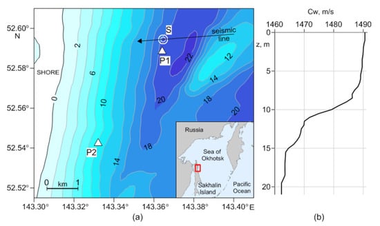
Figure 1.
Map of the seismic survey area with indication of one of the sound emission point S and two reception points P1 and P2 (a). The measured sound speed profile inside the water layer (b).
Figure 2 shows the waveforms of seismic pulses observed at monitoring points P1 and P2. At the distance of 630 m from the emission point (i.e., at P1), where the water depth is 20 m, the magnitudes of the pulse measured near the bottom reaches 3000 Pa. Its spectrum contains two pronounced maxima at the frequencies of 47 Hz and 125 Hz. The value of the sound exposure level SEL in a one-second interval at the point P1 reaches 168 dB re 1 . Note that the SEL quantity is calculated in the frequency domain (not from the time series) by integration over the frequency interval of 10–400 Hz (see Section 3 below). This allows us to reduce the influence of low-frequency pseudo-noise from the flow around the hydrophone and noises with frequencies above 400 Hz.
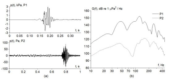
Figure 2.
Variations in acoustic pressure in receivers P1 and P2 (a) and their spectra (b) corresponding to a seismic survey signal emitted at point S.
At the far measurement point P2 located at the distance of 6.2 km from the source, where sea depth is 10 m, the magnitude of the measured pulse does not exceed 90 Pa, and the values of the pulse parameter SEL in a one-second interval decrease to 138.7 dB re . From the waveform of the seismic signal at the point P2, it can be seen that a long low-frequency precursor with a central frequency of 40 Hz is recorded first. This precursor is an interference-type headwave (also known as Buldyrev’s headwave) propagating in the upper layer of bottom sediments. A waterborne component of the pulse is formed behind it, and its energy is mainly distributed over the frequency range of 90–400 Hz.
We use the signal observed at P1 as a reference for reconstructing an effective source spectrum, and the accuracy of reconstruction is validated by the comparison of the waveform recorded at P2 with the simulated pulse computed for this point.
Note that separate air guns used on ships during seismic surveys are combined into arrays (batteries) in order to increase the magnitude of sound pressure and reduce the rate of pulses emission.
In addition, the combination of airguns allows to direct major part of the low-frequency (5–120 Hz) sound energy into the bottom. However, another part of the acoustic energy also propagates in the horizontal directions by exciting waterborne and water-bottom normal modes.
The respective component of the survey pulse can be recorded by hydrophones at the bottom at some distance from the transmitting system. According to field measurements taken at the reception point P1, 91% of the acoustic energy of the recorded pulse is concentrated in the frequency range of 10–200 Hz. The value of the total sound exposure corresponding to the entire pulse near the bottom at the point P1 exceeds the value of the signal energy in the frequency range of 10–200 Hz by just 0.5 dB. Thus, when performing modeling of the seismic survey signal propagation (see Section 3, Section 4 and Section 5), we will restrict ourselves to the frequency range from 10 to 200 Hz.
Note that although in actual experiments the pulses were received by 5 different recorders, we have a permission to present the measurement results from only two of them.
3. Modeling Techniques
In this section we discuss the two approaches used in the present study for the modelling of broadband signals propagation. Both methods are based on the mode parabolic equations (MPE) theory that goes back to works of Collins [10] and Trofimov [17]. This theory was further developed in [11,12,13,14,18]. In particular, Trofimov et al. [14] developed a narrow-angle MPE theory with mode interaction (MPE-MI) taken into account. Although this method was successfully used to solve many practical and idealized problems, it was clear that it is not capable of handling horizontal aperture of the source of more than . This can be clearly seen when solving cross-slope propagation problem for the standard wedge benchmark case. On the other hand, pseudodifferential MPE (PDMPE) from [12,13] can handle arbitrarily wide angles in the horizontal plane, and yet this method is not capable of taking mode interaction into account so far. Both methods however ensure high-speed computations as compared to, e.g., 3D parabolic equation models. We also expect that these methods are somewhat more accurate as compared to the techniques based on rays/Gaussian beams, especially in cases when sea depth is comparable to the wavelength.
Now we briefly describe the two MPE-based approaches to the simulation of sound propagation mentioned above. In both of them acoustic field of a pulse signal in the frequency domain is represented in the form of a modal expansion
where is the source spectrum, are normal modes computed at a vertical cross-section of the considered shallow-water waveguide for a given pair of horizontal coordinates (the corresponding eigenvalues are denoted hereafter as ), and are the so-called mode amplitudes.
Many standard methods can be used to obtain from acoustic spectral problem [19], and afterwards the only remaining task is to compute the amplitudes . Once these functions are known, the distribution can be computed for the given frequency . After repeating such calculations for certain vector of frequencies we can evaluate the waveform of the pulse signal at the receiver by using Fourier transform [19] (note that we use hats over functions in order to emphasize that they are defined in the frequency domain).
3.1. Narrow-Angle Mode Parabolic Equation with Mode Coupling
Within the MPE-MI approach developed by Trofimov et al. [14] the principal oscillation in mode amplitudes is cancelled out according to the formula
where the phase can be obtained by a standard cumulative integral
A system of coupled narrow-angle parabolic equations for smooth envelope functions of mode amplitudes can be written as [14]
3.2. Adiabatic Wide-Angle Mode Parabolic Equation
Introducing the reference modal eigenvalue and cancelling out the principal oscillation from by the substitution
we can show that the envelope function satisfies the so-called pseudo-differential mode parabolic equation (PDMPE) [12,13]
where .
On a small interval of length the PDMPE (3) can be formally solved as
A -Padé approximant of the exponential on the right-hand side of the latter formula (known as the propagator) can be written in the form of a partial fraction expansion as
and hence the solution of the PDMPE (3) can be advanced in x-direction by
4. Source Spectrum Reconstruction and Computation of the SEL Distribution
Equation (1) expresses the solution of the direct problem of sound propagation, i.e., it allows to compute acoustic field due to a point source emitting a signal with the waveform (and the spectrum , where is the Fourier transform). In practice, however, the source waveform is unknown. In order to obtain the SEL distribution we need to estimate using reference measurements. In the experiment considered in this study we use the signal recorded at the point P1 for this purpose. After estimating effective we can use the Equation (1) to compute the field in the frequency domain by solving MPEs.
Assume that we observe signal in the recording made at . We can compute by using its spectrum and the formula
where the denominator is computed by solving MPEs for a discrete set of frequencies uniformly distributed over a given interval (the frequency band).
SEL for the frequency band can be computed using the frequency-domain representation of acoustic field by the following formula
where , , and is the time window size for frequency-domain analysis (in our case ).
5. Simulation Results
The geoacoustic waveguide model used in the simulation of sound propagation along the acoustic path S-P1-P2 consists of two layers (water column and bottom sediments). A realistic bathymetry profile is used in our simulations. The bottom consists of the three sublayers as shown in Figure 3. The sound speed, the density of the sediments, and the attenuation coefficient in the bottom are approximated by piecewise-linear functions of the depth z (cf. Figure 3). This model is based on the estimates of the bottom parameters made during the previous work in this area (see [20]), and we slightly adjusted it to the input format of the Ample and MPE programs used in the simulations. Elastic properties of the bottom are not taken into account, since the bedrock emerges deeper than the considered lower boundary of the waveguide. The sound speed profile in the water column is obtained from in-situ CTD measurements.
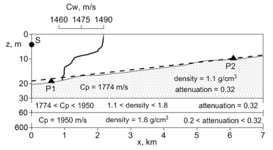
Figure 3.
Waveguide model in the considered example, and the values of acoustic parameters of the media.
Sound source (an array of airguns) is located at the depth of 4 m. The duration of the model signal is 1 s, excluding precursors.
In this section we investigate the differences between the two models described in Section 3 in order to draw a conclusion on which of them is more adequate for solving acoustic monitoring problems.
5.1. Effective Wedge (Averaged Bottom Slope)
As can be seen from Figure 1, isobaths in the area of interest are almost equidistant parallel straight lines, and therefore the bathymetry in the computational domain can be approximated by a linear function. The bottom inclination slope angle is about which is typical for Sakhalin shelf. The propagation path S-P1-P2 is aligned at the angle of about to the x axis, i.e., almost in the cross-slope direction. From the literature it is known that in such environments mode coupling is almost negligible, while horizontal refraction can play an important role in the SEL distribution.
We start with a waveguide model with the bottom approximated by a by a sloping plane described by the following equation:
Using this simple model we investigate the difference between SEL predictions obtained by the narrow-angle MPE model and wide-angle AMPLE program.
Figure 4 shows the horizontal distribution of the SEL parameter of a pulse signal propagating from point S in a waveguide with the bathymetry described by Equation (9), calculated by the Ample (subplot (a)) and the MPE methods (subplot (b)). Subplot (c) corresponds to the modulus of the difference of these SEL distributions. Calculations indicate that at depths less than 10 m, the field difference exceeds 8 dB. It is clear that Ample (as compared to the MPE model) allows to better reproduce the effect of horizontal refraction of sound over the sloping bottom. SEL difference is significant enough to conclude that in propagation scenarios similar to the one considered here it is important to use a model that has sufficiently wide aperture in the horizontal plane.
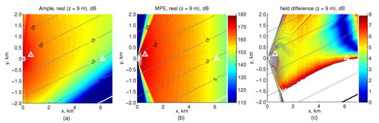
Figure 4.
Spatial distribution of the SEL parameter at a horizon of 9 m, calculated by Ample (a) and MPE (b) for the waveguide model with the bottom slope given by Equation (9). SEL difference modulus is also shown (c).
5.2. Realistic Bathymetry
Let us now investigate the accuracy of SEL computations by the two models by using realistic bathymetry data in our geoacoustic waveguide model. In this case we can also simulate the waveform of the signal at the point P2 and evaluate the accuracy of the model by a direct comparison with measurements data.
Figure 5, Figure 6 and Figure 7 show calculation results in the case of realistic bathymetry. Contour plots in Figure 5 show that SEL distribution patterns in this case are qualitatively similar to the ones obtained using a simplified bathymetry model (9). Note that the difference between the two models (Figure 5c) in this case also resembles the contour plot in Figure 4c. SEL distributions clearly reflect bathymetry features in the area, and their patterns show typical manifestation of the horizontal refraction in a shallow-water environment (noticeably greater field magnitude in the deeper part of the area).
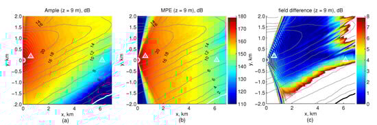
Figure 5.
Spatial distribution of the SEL parameter at a horizon of 9 m, calculated by Ample (a) and MPE (b) for realistic bathymetry. Field difference module (c).
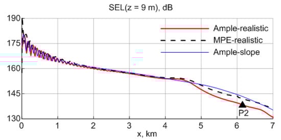
Figure 6.
The dependence of the SEL on the range x at the depth of 9 m calculated by Ample and MPE for realistic and linear bathymetry.
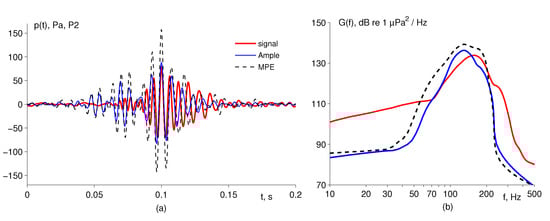
Figure 7.
Comparison of filtered experimental and model pulse signals at the reception point P2 (a) and their spectra (b).
Also note that the results obtained using Ample and MPE exhibit relatively good agreement along the path (i.e., along the line ) (see Figure 6 and also Figure 5c along the x axis). However, stepping aside from this line we observe significant differences in the results produced by the two models (see Figure 5c). Clearly, this difference results from the limited aperture of the MPE in the horizontal plane, and it is important to note that it reaches 8 dB even within the sector (about the line ) at the distance of ca. 7 km from the source.
A final validation of both models is accomplished by direct comparison of the pulse signal waveforms at the point P2 (recall that the source spectrum is reconstructed using the data from the point P1). This comparison in presented in Figure 7). The pulse obtained using Ample program exhibits significantly better agreement to the signal observed in the experiment.
Similar results were obtained for other recorders used in our measurements program, however, as was mentioned earlier, we don not have the permission to present them in this publication.
6. Conclusions and Future Work
In this study we outlined and validated an algorithm for estimating SEL distribution over a large sea area in the course of acoustical monitoring of anthropogenic noises of various origins (e.g., pile driving and seismic survey). In our algorithm, one recording unit (with a hydrophone) deployed in the area of interest is used for reconstructing effective source spectrum, and the MPE theory is used for computing the field and SEL in the entire area.
The proposed approach is illustrated by using measurements data collected in the Sea of Okhotsk on the Sakhalin shelf. In the considered setup, seismic pulses emitted by a survey vessel were recorded by the two receivers deployed near the vessel track. Pulses recorded by a receiver P1 located ca. 600 m from the emission point S were used for the source spectrum reconstruction, while the data from the other receiver P2 were used for the comparison with the simulation results and validation of the accuracy of SEL modeling.
It was shown that our approach allows to reproduce the pulse waveform at P2 with reasonable accuracy, both in time- and in frequency-domain. It is also important to note that pseudo-differential (wide-angle) adiabatic MPE produces significantly more accurate results than its narrow-angle counterpart, even if the mode interaction is taken into account. Despite the fact that total SEL of the signal in our simulation is reproduced with accuracy sufficient for practical applications (as we can from the direct comparison at the point P2), we still observe substantial disagreement of spectra for the frequency range 10–50 Hz (as can be seen from Figure 7). This disagreement can be explained by the lack of knowledge about the layers constituting the sea bottom. It would be appropriate to incorporate a geoacoustic inversion algorithm into our software, so that the structure of bottom layers is also reconstructed on the basis of measurements data. Indeed, the dispersion data of broadband seismic survey pulses obtained from acoustic measurements taken few kilometers away from the source (e.g., at P2 in our case) can be used to perform the inversion by a warping-based method [21]. This would further improve the quality of SEL distribution modeling. Of course, even in this case the inverted parameters of the bottom layers would only be a path-averaged rough approximations to their counterparts in real marine environment, and some important 3D effects arising from the variations of bottom parameters along and across the pass [22] still would be neglected.
The question of choosing adequate mathematical methods for 3D modeling of sound propagation in cases when the computational cost is as important as the accuracy is still open. In recent study [23] a comprehensive comparison of several important approaches and respective computational codes was presented, and it was shown that in many cases Gaussian beams [24] can be an attractive option. In our opinion however the advantages and shortcomings of the MPE-based technique are somewhat better balanced, though some additional work still has to be done in order to include mode interaction [14] into the model from [12].
Author Contributions
Methodology, P.P.; data analysis and numerical simulations, D.M. and M.F.; software development, A.T. and P.P.; writing (original draft), D.M.; writing and editing: all authors. All authors have read and agreed to the published version of the manuscript.
Funding
This study was supported by POI FEB RAS Program “Modeling of various-scale dynamical processes in the ocean” (project No. 121021700341-2) and “Study of the fundamental foundations of the origin, development, transformation and interaction of hydroacoustic, hydrophysical and geophysical fields of the World Ocean” (project No. AAAA-A20-120021990003-3). MPE and Ample software was developed with support of Exxon Neftegas Limited.
Institutional Review Board Statement
Not applicable.
Informed Consent Statement
Not applicable.
Data Availability Statement
Not applicable.
Conflicts of Interest
The authors declare no conflict of interest.
References
- Rutenko, A.; Borisov, S.; Gritsenko, A.; Jenkerson, M. Calibrating and monitoring the western gray whale mitigation zone and estimating acoustic transmission during a 3D seismic survey, Sakhalin Island, Russia. Environ. Monit. Assess. 2007, 134, 21–44. [Google Scholar] [CrossRef] [PubMed] [Green Version]
- Nowacek, D.P.; Bröker, K.; Donovan, G.; Gailey, G.; Racca, R.; Reeves, R.R.; Vedenev, A.I.; Weller, D.W.; Southall, B.L. Responsible practices for minimizing and monitoring environmental impacts of marine seismic surveys with an emphasis on marine mammals. Aquat. Mamm. 2013, 39, 356. [Google Scholar] [CrossRef] [Green Version]
- Rutenko, A.; Borovoi, D.; Gritsenko, V.; Petrov, P.; Ushchipovskii, V.; Boekholt, M. Monitoring the acoustic field of seismic survey pulses in the near-coastal zone. Acoust. Phys. 2012, 58, 326–338. [Google Scholar] [CrossRef]
- Bailey, H.; Brookes, K.L.; Thompson, P.M. Assessing environmental impacts of offshore wind farms: Lessons learned and recommendations for the future. Aquat. Biosyst. 2014, 10, 1–13. [Google Scholar] [CrossRef] [PubMed] [Green Version]
- Racca, R.; Austin, M.; Rutenko, A.; Bröker, K. Monitoring the gray whale sound exposure mitigation zone and estimating acoustic transmission during a 4-D seismic survey, Sakhalin Island, Russia. Endanger. Species Res. 2015, 29, 131–146. [Google Scholar] [CrossRef] [Green Version]
- Lucke, K.; Martin, S.B.; Racca, R. Evaluating the predictive strength of underwater noise exposure criteria for marine mammals. J. Acoust. Soc. Am. 2020, 147, 3985. [Google Scholar] [CrossRef]
- Bröker, K.C. Monitoring and Mitigation of the Sound Effects of Hydrocarbon Exploration Activities on Marine Mammal Populations. Ph.D. Thesis, University of Groningen, Groningen, The Netherlands, 2021. [Google Scholar]
- Rutenko, A.; Gritsenko, V.; Kovzel, D.; Manulchev, D.; Fershalov, M.Y. A Method for Estimating the Characteristics of Acoustic Pulses Recorded on the Sakhalin Shelf for Multivariate Analysis of their Effect on the Behavior of Gray Whales. Acoust. Phys. 2019, 65, 556–566. [Google Scholar] [CrossRef]
- Lin, Y.T.; Duda, T.F.; Newhall, A.E. Three-dimensional sound propagation models using the parabolic-equation approximation and the split-step Fourier method. J. Comput. Acoust. 2013, 21, 1250018. [Google Scholar] [CrossRef] [Green Version]
- Collins, M.D. The adiabatic mode parabolic equation. J. Acoust. Soc. Am. 1993, 94, 2269–2278. [Google Scholar] [CrossRef]
- Abawi, A.T.; Kuperman, W.A.; Collins, M.D. The coupled mode parabolic equation. J. Acoust. Soc. Am. 1997, 102, 233–238. [Google Scholar] [CrossRef]
- Petrov, P.S.; Ehrhardt, M.; Tyshchenko, A.G.; Petrov, P.N. Wide-angle mode parabolic equations for the modelling of horizontal refraction in underwater acoustics and their numerical solution on unbounded domains. J. Sound Vib. 2020, 484, 115526. [Google Scholar] [CrossRef]
- Petrov, P.S.; Antoine, X. Pseudodifferential adiabatic mode parabolic equations in curvilinear coordinates and their numerical solution. J. Comput. Phys. 2020, 410, 109392. [Google Scholar] [CrossRef] [Green Version]
- Trofimov, M.Y.; Kozitskiy, S.; Zakharenko, A. A mode parabolic equation method in the case of the resonant mode interaction. Wave Motion 2015, 58, 42–52. [Google Scholar] [CrossRef]
- Tyshchenko, A.; Zaikin, O.; Sorokin, M.; Petrov, P. A Program based on the Wide-Angle Mode Parabolic Equations Method for Computing Acoustic Fields in Shallow Water. Acoust. Phys. 2021, 67, 512–519. [Google Scholar] [CrossRef]
- Rutenko, A.; Borisov, S.; Kovzel, D.; Gritsenko, V. A radiohydroacoustic station for monitoring the parameters of anthropogenic impulse and noise signals on the shelf. Acoust. Phys. 2015, 61, 455–465. [Google Scholar] [CrossRef]
- Trofimov, M.Y. Narrow-angle parabolic equations of adiabatic single-mode propagation in horizontally inhomogeneous shallow sea. Acoust. Phys. 1999, 45, 575–580. [Google Scholar]
- Trofimov, M.Y. Wide-angle mode parabolic equations. Acoust. Phys. 2002, 48, 728–734. [Google Scholar] [CrossRef]
- Jensen, F.B.; Kuperman, W.A.; Porter, M.B.; Schmidt, H. Computational Ocean Acoustics; Springer: New York, NY, USA, 2011. [Google Scholar]
- Rutenko, A.; Gavrilevsky, A.; Putov, V.; Soloviev, A.; Manulchev, D. Monitoring of anthropogenic noise on the shelf of the Sakhalin Island during seismic surveys. Acoust. Phys. 2016, 62, 348–362. [Google Scholar] [CrossRef]
- Bonnel, J.; Thode, A.; Wright, D.; Chapman, R. Nonlinear time-warping made simple: A step-by-step tutorial on underwater acoustic modal separation with a single hydrophone. J. Acoust. Soc. Am. 2020, 147, 1897–1926. [Google Scholar] [CrossRef] [Green Version]
- Lunkov, A.; Sidorov, D.; Petnikov, V. Horizontal Refraction of Acoustic Waves in Shallow-Water Waveguides Due to an Inhomogeneous Bottom Structure. J. Mar. Sci. Eng. 2021, 9, 1269. [Google Scholar] [CrossRef]
- Oliveira, T.C.; Lin, Y.T.; Porter, M.B. Underwater sound propagation modeling in a complex shallow water environment. Front. Mar. Sci. 2021, 8, 751327. [Google Scholar] [CrossRef]
- Porter, M.B. Beam tracing for two-and three-dimensional problems in ocean acoustics. J. Acoust. Soc. Am. 2019, 146, 2016–2029. [Google Scholar] [CrossRef] [PubMed]
Publisher’s Note: MDPI stays neutral with regard to jurisdictional claims in published maps and institutional affiliations. |
© 2022 by the authors. Licensee MDPI, Basel, Switzerland. This article is an open access article distributed under the terms and conditions of the Creative Commons Attribution (CC BY) license (https://creativecommons.org/licenses/by/4.0/).