Development of a Computational Model for Investigation of and Oscillating Water Column Device with a Savonius Turbine

Abstract

The present work aims to develop a computational model investigating turbulent flows in a problem that simulates an oscillating water column device (OWC) considering a Savonius turbine in the air duct region. Incompressible, two-dimensional, unsteady, and turbulent flows were considered for three different configurations: (1) free turbine inserted in a long and large channel for verification/validation of the model, (2) an enclosure domain that mimics an OWC device with a constant velocity at its inlet, and (3) the same domain as that in Case 2 with sinusoidal velocity imposed at the inlet. A dynamic rotational mesh in the turbine region was imposed. Time-averaged equations of the conservation of mass and balance of momentum with the k–ω Shear Stress Transport (SST) model for turbulence closure were solved with the finite volume method. The developed model led to promising results, predicting similar time–spatial-averaged power coefficients ($\overline{C_P}$) as those obtained in the literature for different magnitudes of the tip speed ratio (0.75 ≤ λ ≤ 2.00). The simulation of the enclosure domain increased $\overline{C_P}$ for all studied values of λ in comparison with a free turbine (Case 1). The imposition of sinusoidal velocity (Case 3) led to a similar performance as that obtained for constant velocity (Case 2).

1. Introduction

The energy demand will increase by more than 1.0% per year up to 2040, increasing gases emission rates [1]. Moreover, the costs of commodities for energy generation from fossil fuels have increased significantly, leading to economic difficulties, risks associated with energy security, and geopolitical conflicts around the world [2]. Considering this scenario, there is a growing search for a better comprehension of the development of technologies and the use of devices and economic impacts of different renewable sources of energy such as wind, solar, geothermal, and ocean energy [2,3,4,5,6,7,8,9,10,11].

One of the important sources of renewable energy with high potential, but not frequently explored worldwide, is the conversion of ocean energy into electricity [12,13,14,15], i.e., wave energy conversion. Despite several signs of progress in technological development, there is no dominant main operational principle. Several devices have been proposed and investigated based on various ways to convert wave energy such as point absorbers, attenuators, oscillating surge converters, overtopping, submerged plates, and oscillating water columns (OWCs) [12,13,14]. The efficiency and survivability of the wave energy converters (WECs) are important issues to make them more competitive and viable [16]. In this context, the OWC device has advantages as its simplicity and maintenance, e.g., the moving parts are located outside of the water, increasing the lifetime material of the power take-off (PTO) system, and the structures of buildings are robust [12,13,14]. Therefore, several studies and prototypes using the OWC as the main operational principle have been developed around the world: Sakata–Japan (60 kW), Mutriku–Spain (296 kW), Pico–Portugal (400 kW), Tofteshallen–Norway (500 kW), Islay island–Scotland (500 kW), and Lewis island–Scotland (4.0 MW) [17,18,19,20,21,22].

Important experimental works have sought to improve the comprehension of the fluid dynamic behavior of water/air flow in the OWC device and investigate the influence of some parameters over its performance. For instance, experiments in the laboratory and large-scale domains analyzed the influence of the inclination of the frontal wall, entrance areas of the OWC chamber, and water depth on the device efficiency, reflection, and loading of an OWC for different wave conditions [23,24,25]. Recently, the experimental progress extended to understand the hydrodynamic of the fluid flow into dual chambers OWC [26,27].

The numerical simulation of OWC devices has also been worth investigating. Several works have been performed since the development of computational models to represent the main operating principle of the device and the investigation of several parameters regarding the performance. For the former purpose, the representation of fluid flow in a laboratory and large-scale devices has been done without considering the effect of a turbine, as in Maciel et al. [28]. Other studies have considered it using orifice plates, plate-baffle, obstacles, or actuator disks to simulate the head loss caused by the turbine over the airflow in the hydropneumatic chamber and air duct of the device [29,30,31,32,33]. Recently, an interesting approach employed the numerical simulation of water and air in the chamber and considered the effects of Wells and impulse turbines by means of analytical thermodynamic models [34,35]. All models mentioned above have been used to obtain recommendations about parameters such as the depth and inclination of the frontal wall, height and length of the chamber, the diameter of the turbine, ramp placed in the seabed below the OWC chamber, and, recently, the design of multiple coupled chambers regarding device performance for different scales and wave conditions [24,32,35,36,37,38,39,40]. It is also worth mentioning the efforts made to represent the sea state in a more trustworthy form. In this field, some studies modeled the irregular waves using a wave spectrum such as JONSWAP, and others obtained the sea state from geophysical models such as TOMAWAC and used this as an input for the modeling of a channel with the device to be investigated [41,42,43].

Some significant advancements regarding the PTO of OWC have also been reported in the literature. For instance, Britto-Melo et al. [44] numerically investigated the influence of the aerodynamic parameters of the Wells turbine and the influence of guide vanes and the bypass valve on the pressure drop, torque, and the overall performance. In this work, the conversion of pneumatic energy into electrical energy was estimated with a computational model based on the results extrapolated from aerodynamic tests on a scale model and empirical approximations for the generator losses. Recently, Rodríguez et al. [45] proposed a computational study to understand the behavior of OutFlow Radial (OFR) turbines in both direct and reverse modes, simulating an axisymmetric domain with the flow between a blade-to-blade arrangement of the turbine. The authors observed that the outer blade angle had poor performance in reverse mode despite the improvement of the global performance due to the rotor efficiency gain in direct mode. However, there are few studies related to the numerical simulation of the OWC device turbine considering the rotational domain with the intruded turbine rotor. Prasad et al. [46] performed similar work in this direction and developed a numerical model with a Savonius turbine immersed in a channel under regular wave flow, simulating a hydrokinetic turbine. The authors also investigated the influence of some parameters such as the submergence and the rotational speed for different blade entry angles regarding the rotor power.

Despite the several above-mentioned contributions, to the authors’ knowledge, the development of computational models for the simulation of OWC devices considering the rotational turbine in the air duct is an approach still little explored in the literature. Recently, however, Liu et al. [47] presented the validation of an integrated three-dimensional numerical model considering an axial-flow impulse turbine coupled with an OWC inserted in a numerical wave tank (NWT). The present work aims to perform the first step in this direction. Initially, turbulent air flow over a free turbine inserted in a long and large channel (commonly used to represent the numerical modeling of wind turbines) was simulated to verify/validate the present model (Case 1). The effect of the tip speed ratio (λ) on the time and spatial averaged power coefficient ($\overline{C_P}$) of a Savonius turbine was compared with numerical and experimental results available in the literature [48,49], investigating the tip speed ratios in the range 0.75 ≤ λ ≤ 2.00. An enclosure domain that mimics an OWC device was simulated considering a constant velocity imposed at the inlet of the domain (Case 2) and sinusoidal velocity that simulated the alternate flow in an OWC device (Case 3). For all cases, the influence of λ on the turbine performance and aerodynamic coefficients was investigated.

Moreover, incompressible, two-dimensional, unsteady, and turbulent flows with Re_D = 867,000 were considered. URANS (Unsteady Reynolds-Averaged Navier Stokes) modeling was applied to all cases. Time-averaged equations of the conservation of mass, the balance of momentum, and transport equations of the k–ω SST model (used in the closure of turbulence) were solved with the finite volume method (FVM) [50,51,52,53,54,55], using the commercial code Ansys FLUENT 14.5 [56].

2. Mathematical Modeling

Incompressible, two-dimensional, unsteady, turbulent flows with constant thermo-physical properties were considered. It is worth mentioning that one of the characteristics of turbulence is the three-dimensional structure of the flow [57]. Despite this fact, the present simulations represent most of the characteristics of turbulent flows, and the modeling properly predicts the transient behavior of parameters such as drag, lift, moment, and power in the Savonius turbine.

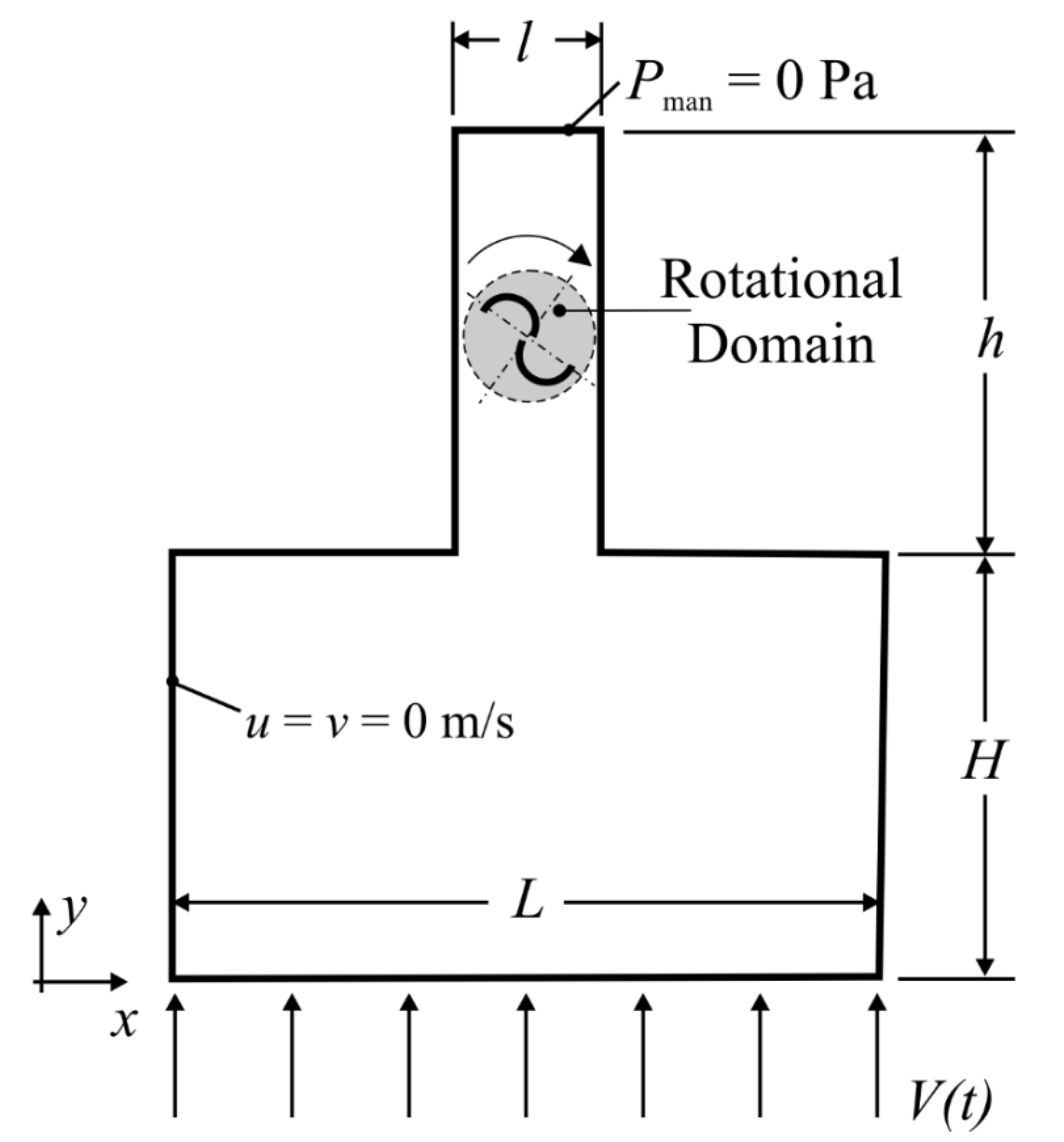
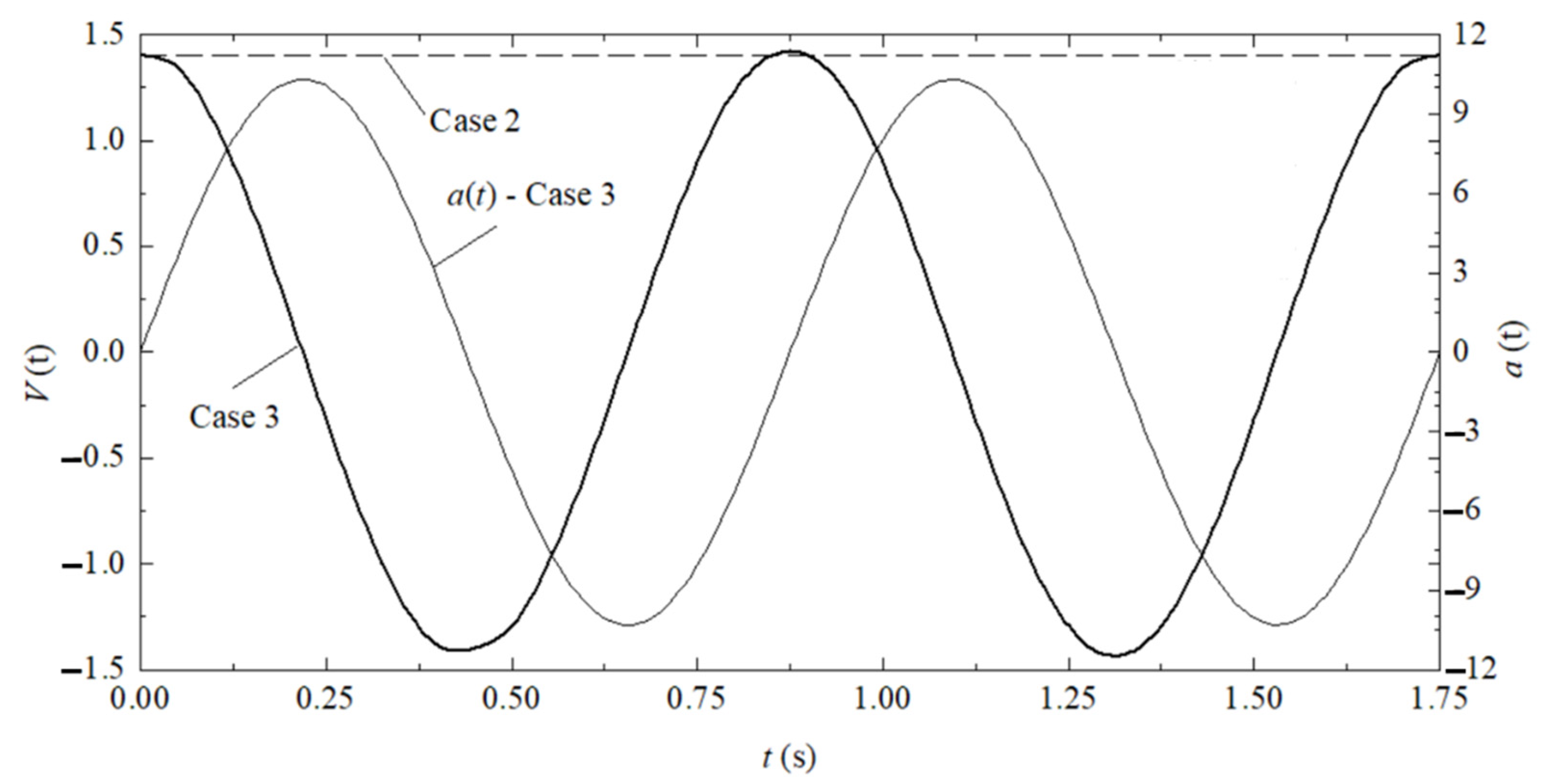
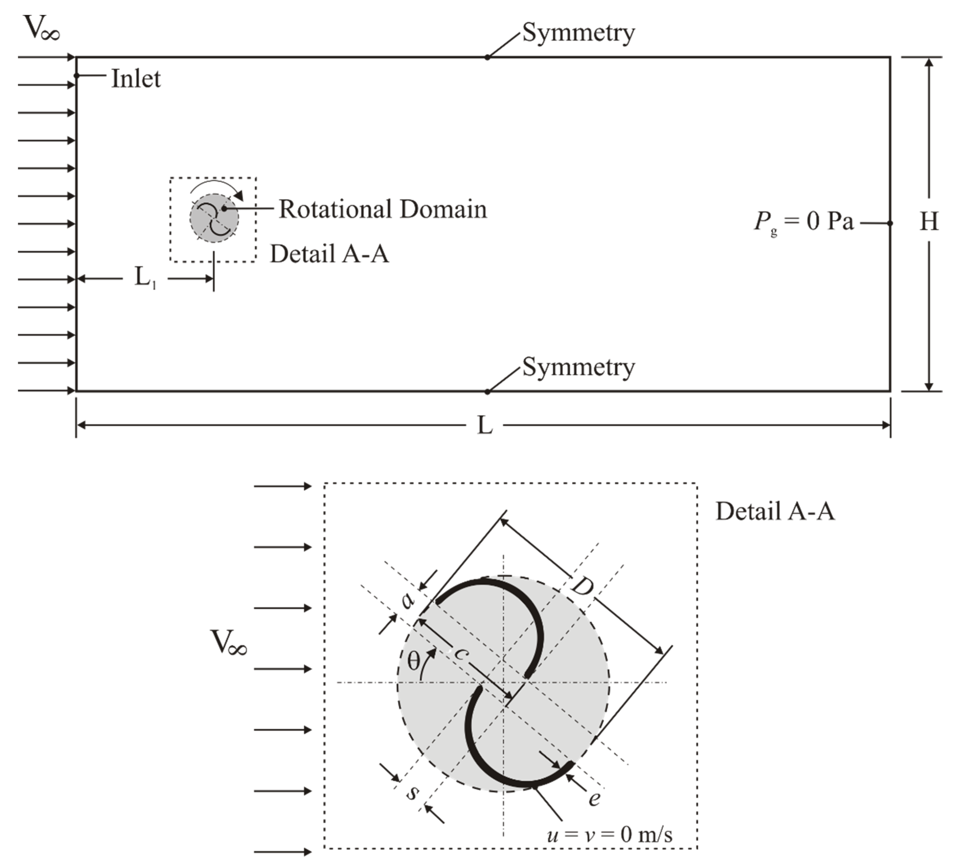
2.1. Description of the Studied Cases

Figure 1 illustrates the computational domain of Case 1 used for verification/validation of the present model. The domain consists of a long and large channel with an inserted free Savonius turbine. The dimensions are similar to those investigated in the work of Akwa et al. [49]. In this case, the fluid flow of air is caused by the imposition of a constant velocity (V_∞) at the inlet (left side surface). On this surface, there is also an imposed turbulent intensity of IT = $\sqrt{\overline{{u^{\prime }}^2}}/\overline{u}={\sigma }_u/\overline{u}$ = 1.0%, where u’ is the fluctuation of the velocity field, $\overline{u}$ is the time-averaged velocity field, and σ_u represents the variance of u’. At the exit of the channel (right side surface), there is an imposed null gauge pressure (p_g = 0 atm). At the upper and lower surfaces, there is a free slip and impermeability boundary condition (also called symmetry). In the turbine region, there is an imposed constant angular velocity (n) in the gray region named the “Rotational Domain” simulating the effect of wind action over the turbine. In the turbine walls, there is an imposed no-slip and impermeability boundary condition (u = v = 0 m/s) related to the rotational domain. Figure 1 illustrates the details of the turbine region with the geometric variables used to design it.

Table 1. Parameters used in the verification/validation case (Case 1).

Parameter	Magnitude
Air density: ρ (kg/m³)	1.1845
Dynamic viscosity: μ (kg/ms)	1.7894 × 10−5
H (m)	21.6 (12D)
L (m)	46.8 (26D)
L1 (m)	10.8 (6D)
D (m)	1.8
V∞ (m/s)	7.0
Turbulence intensity: IT (%)	1.0
ReD = ρV∞D/μ	867,000
c (m)	0.972
a (m)	0.0
e (m)	7.2 × 10−3
s (m)	0.144
Tip speed ratio: λ	0.75	1.00	1.25	2.00
Angular velocity of turbine: n (rad/s)	5.83	7.77	9.72	15.54
Time of simulation and statistics analysis (s)	3.50 s		1.75 s

presents the parameters of the fluid flow, thermo-physical properties, dimensions of the computational domain, and turbine variables used here for the four different tip speed ratios of the rotor (λ = nD/2V_∞) of λ = 0.75, 1.00, 1.25, and 2.00; n is the angular velocity of the turbine and D is the turbine diameter. For the unsteady analysis, there was a time interval of t_f = 3.5 s, with the last 1.75 s being analyzed for computation of the drag, lift, momentum, and power coefficients.

Figure 2 illustrates the computational domain used in Case 2 and Case 3. These cases were defined based on Case 1. Therefore, the thermo–physical properties and dimensions of the turbine were the same, presented in Table 1 (Case 1). The main differences here are the domain dimensions (H = h = 6.0 m, L = 10.0 m, and l = 2.0 m) and the insertion of the Savonius turbine in an enclosure domain, leading to the imposition of a no-slip and impermeability boundary condition (u = v = 0 m/s) in the device walls. At the lower surface, there was an imposed constant velocity of V(t) = 1.4 m/s and IT = 1.0% for Case 2. The magnitude of the imposed velocity was defined in such a way to have a value of 7.0 m/s at the inlet of the air duct (in the contraction from the chamber to the air duct), leading to a Reynolds number in the turbine similar to that reached for Case 1. For Case 3, the sole difference in comparison with Case 2 was the imposition of a sinusoidal function that mimicked the oscillating behavior in the OWC chamber:

$$V\left(t\right)=\frac{H_w\pi }{T_w}\cos \left(\frac{2\pi t}{T_w}\right)$$

(1)

where H_w = 0.4 m, T_w = 0.875 s, allowing the reproduction of the piston-type movement generated by the regular waves incidence over the OWC. The range of magnitudes was limited by (−1.4 m/s ≤ V(t) ≤ 1.4 m/s). The use of real configurations of a sea wave, for example, leads to long periods of simulation, requiring a high computational effort. As the purpose of this case is to compare the imposition of the sinusoidal velocity profile with the case with constant velocity to investigate the effect of oscillating flow over the device parameters and performance, the idealized imposed velocity variation was adequate for the desired investigation. For Case 2 and Case 3, the same four magnitudes of the tip speed ratio studied in the verification/validation case (λ = nD/2V₁) of λ = 0.75, 1.00, 1.25, and 2.00 were investigated. It is worth mentioning that a mean velocity was measured in the air duct and before the turbine (V₁) for the calculation of λ.

In the present work, results the influence of λ over the drag, lift, moment, and power coefficients (C_d, C_l, C_T, and C_P) are based on [57]:

$$C_d=\frac{F_d}{1/2\rho A_r{V}^2}$$

(2)

$$C_l=\frac{F_l}{1/2\rho A_r{V}^2}$$

(3)

$$C_T=\frac{T}{1/2\rho A_r{V}^{2}r}$$

(4)

$$C_P=\frac{P}{P_{available}}=\frac{T}{1/2\rho A_r{V}^{2}r}\frac{rn}{V}=C_T\lambda$$

(5)

where F_d is the drag force (N), F_l is the lift force (N), T is the rotor moment (N∙m), A_r is the projected area of the Savonius rotor (A_r = D∙W), W is the depth of the domain in the z-direction (m), V is the upstream turbine velocity (V = V_∞ for the Case 1 and V = V₁ for Case 2 and Case 3) (m/s), r is the radius of the rotor (m), P is the turbine power (W), and P_available is the available power of the wind upstream of the rotor (W).

It is worth mentioning that the use of Equation (5) is valid only for the prediction of power coefficients in turbines subjected to open flow conditions (seen in tidal or wind power devices). In OWC devices, the air flow is driven by the pneumatic power, i.e., the pressure drop in the device must also be taken into account. Therefore, for power coefficients predicted for the enclosure domain of Case 2 and Case 3, the C_P is calculated as:

$$C_P=\frac{P}{P_{pneumatic}}=\frac{P}{\left(\Delta p+\frac{\rho V^2}{2}\right)Q}$$

(6)

where Δp is the pressure drop between the OWC chamber and the exit of the chimney (Pa), V is the air velocity at the OWC turbine-duct (m/s) (V = V₁), and Q is the volumetric flow rate of the air (m³/s).

The time-averaged magnitudes of the drag, lift, moment, and power coefficients are obtained as follows:

$$\overline{C_{d,l,T,P}}=\frac{1}{t_f}{\displaystyle \underset{0}{\overset{t_f}{\int }}{C}_{d,l,T,P}}dt$$

(7)

2.2. Governing Equations of Turbulent Flows

For all simulations, the modeling of incompressible, two-dimensional, unsteady, and turbulent flows is given by the time-averaged conservation equation of mass and balance of momentum in the x and y directions and can be written as [50,51]:

$$\frac{\partial \overline{u}}{\partial x}+\frac{\partial \overline{v}}{\partial y}=0$$

(8)

$$\rho \left[\frac{\partial \overline{u}}{\partial t}+\overline{u}\frac{\partial \overline{u}}{\partial x}+\overline{v}\frac{\partial \overline{u}}{\partial y}\right]=-\frac{\partial \overline{p}}{\partial x}+\left(\mu +{\mu }_t\right)\left(\frac{{\partial }^2\overline{u}}{\partial x^2}+\frac{{\partial }^2\overline{u}}{\partial y^2}\right)$$

(9)

$$\rho \left[\frac{\partial \overline{v}}{\partial t}+\overline{u}\frac{\partial \overline{v}}{\partial x}+\overline{v}\frac{\partial \overline{v}}{\partial y}\right]=-\frac{\partial \overline{p}}{\partial y}+\left(\mu +{\mu }_t\right)\left(\frac{{\partial }^2\overline{v}}{\partial x^2}+\frac{{\partial }^2\overline{v}}{\partial y^2}\right)$$

(10)

where x and y are the spatial coordinates (m), u and v are the velocity components in the x and y directions, respectively (m/s), p is the pressure (N/m²), μ is the dynamic viscosity (kg/m∙s), μ_t is the turbulent viscosity (kg/m∙s), and the overbar represents the time-averaged operator.

For the k–ω SST closure model, the turbulent viscosity (μ_t) is [52,53]:

$${\mu }_t=\frac{\overline{\rho }{\alpha }_{1}k}{\max \left({\alpha }_1\omega ,S{F}_2\right)}$$

(11)

The transport equations of turbulent kinetic energy (k) and its specific dissipation rate (ω) are as follows:

$$\frac{\partial k}{\partial t}+\frac{\partial \left({\overline{u}}_{i}k\right)}{\partial x_i}={\tilde{P}}_k-\frac{k^{\raisebox{1ex}{$3$}\!\left/ \!\raisebox{-1ex}{$2$}\right.}}{L_T}+\frac{\partial }{\partial x_i}\left[\left(\mu +{\sigma }_k{\mu }_t\right)\frac{\partial k}{\partial x_i}\right]$$

(12)

$$\frac{\partial \omega }{\partial t}+\frac{\partial \left({\overline{u}}_i\omega \right)}{\partial x_i}=\frac{\alpha }{{\mu }_t}{\tilde{P}}_k-\beta {\omega }^2+\frac{\partial }{\partial x_i}\left[\left(\mu +{\sigma }_{\omega }{\mu }_t\right)\frac{\partial \omega }{\partial x_i}\right]+2\left(1-F_1\right)\frac{{\sigma }_{\omega 2}}{\omega }\frac{\partial k}{\partial x_i}\frac{\partial \omega }{\partial x_i}$$

(13)

where ${\tilde{P}}_k$ is a function that prevents the turbulence generation in stagnation regions, i represents the direction of fluid flow (i = 1 represents the x direction and i = 2 represents the y direction), β = 0.09, α₁ = 5/9, β₁ = 3/40, σ_k = 0.85, σ_w = 0.5, σ₂ = 0.44, β₂ = 0.0828, σ_k2 = 1, σ_w2 = 0.856 are ad hoc constants used in [52]. F₁ and F₂ are blending functions defined as follows:

$$F_1=\tanh \left\{{\left\{\min \left[\max \left(\frac{k^{\raisebox{1ex}{$1$}\!\left/ \!\raisebox{-1ex}{$2$}\right.}}{{\beta }^{*}\omega y},\frac{500\upsilon }{y^2\omega }\right),\frac{4\rho {\sigma }_{\omega 2}k}{C{D}_{k\omega }{y}^2}\right]\right\}}^4\right\}$$

(14)

$$F_2=\tanh \left\{{\left[\max \left(\frac{2k^{\raisebox{1ex}{$1$}\!\left/ \!\raisebox{-1ex}{$2$}\right.}}{{\beta }^{*}\omega y},\frac{500\upsilon }{y^2\omega }\right)\right]}^2\right\}$$

(15)

In Equation (13), the term CD_kω is calculated as follows:

$$C{D}_{k\omega }=\max \left(2\rho {\sigma }_{\omega 2}\frac{1}{\omega }\frac{\partial k}{\partial x_i}\frac{\partial \omega }{\partial x_i},{10}^{-10}\right)$$

(16)

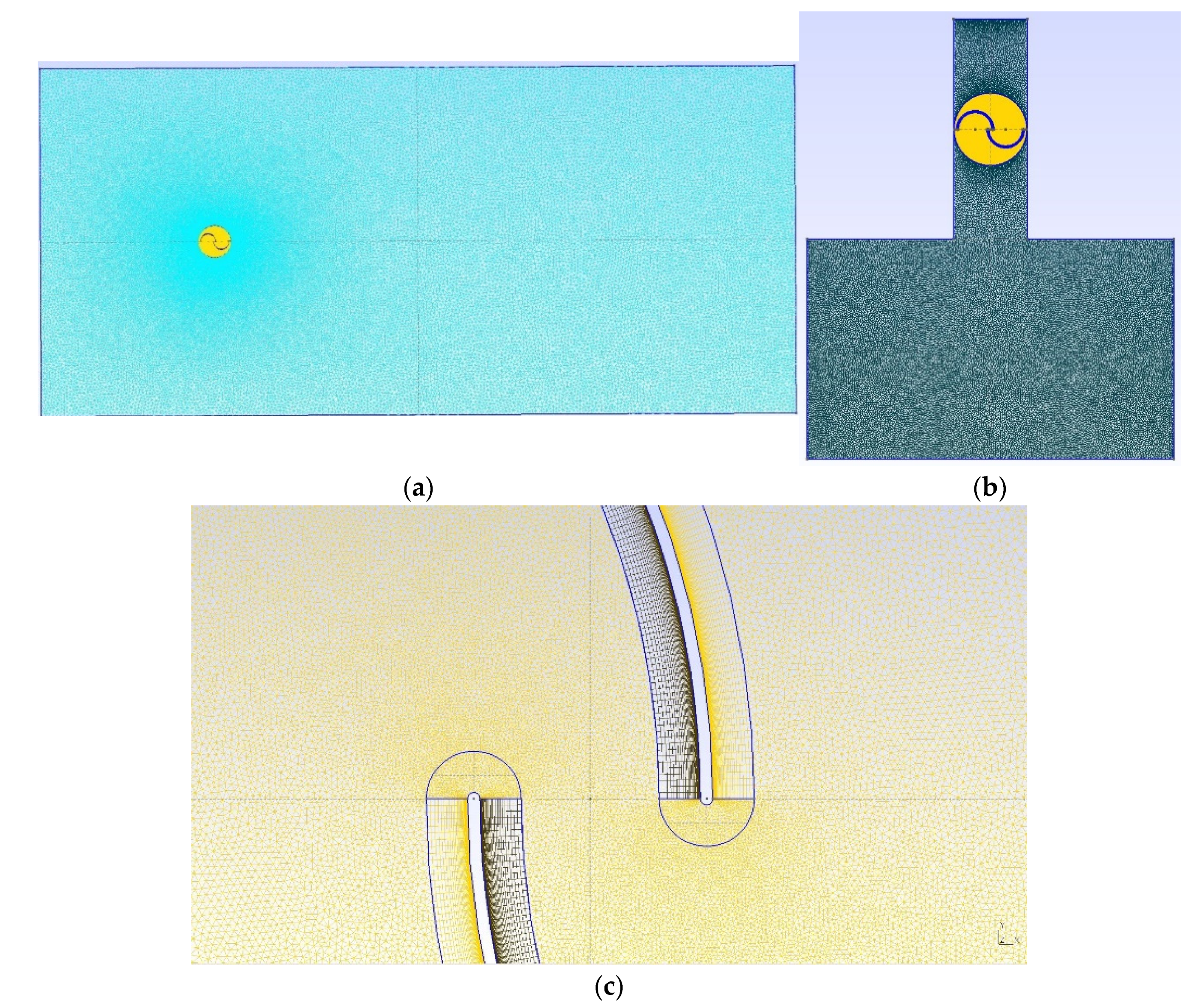
3. Numerical Modeling

The solution of the governing equations was performed with the FVM using the commercial package Ansys Fluent^TM [54,55,56]. To tackle the advective terms of the balance of momentum and transport of k and ω, the second-order upwind interpolation function was employed. The algorithm SIMPLE (Semi-Implicit Method for Pressure Linked Equations) was used for pressure–velocity coupling. The simulations were considered to have converged when the residuals for continuity, the balance of momentum, k and ω transport equations were less than 10⁻⁵. Moreover, the maximum number of iterations per time step was 200. Concerning the time advancement, there was an implicit time advancement scheme and a fixed time step of Δt = 1.75 × 10⁻³ s. All simulations were performed using desktops with six core Intel^® Core ™ i7 5820K @ 3.30 GHz processors and 16 Gb of RAM memory. The processing time for the simulation of t = 3.5 s of physical time was nearly 20 × 10³ s.

Concerning spatial discretization, hybrid triangular and rectangular finite volumes were used with the domain in simulations of Case 1, Case 2, and Case 3. Figure 3a–c illustrates the mesh generated with software GMSH [58] for the free Savonius turbine (Case 1), the configuration similar to the OWC device (Case 2 and Case 3), and a detail of the mesh in the blades of Savonius turbine, respectively. In detail, it is possible to observe a region around the blades with the refined rectangular mesh. The dimensions of the rectangular volumes were defined as a function of a grid independence study and the parameter for representation of the boundary layer (y⁺), which must be y⁺ ≤ 1.0 in the walls; y⁺ was defined as follows [51,52,53]:

$$y^{+}=\frac{y\sqrt{{\tau }_w/\rho }}{\nu }=\frac{y{u}_{\tau }}{\nu }$$

(17)

where y is the normal distance to the wall (m), τ_w is the surface tension in the wall (N/m²), ν is the kinematic viscosity (m²/s), and u_τ is the friction velocity (m/s).

For the grid independence study, four different meshes were simulated, and the results for the time-averaged power coefficient for the free Savonius rotor (Case 1) with Re_D = 867,000, λ = 1.25, and bucket overlap ratio of R_S = s/c = 0.15 are presented in

Table 2. Grid independence test for a free turbine with Re_D = 867,000, λ = 1.25, and R_S = 0.15.

Number of Volumes	$\overline{{\mathit{C}}_{\mathit{P}}}$	Dev (%)
163,141	0.20726	------
168,659	0.21219	2.37 × 100
220,937	0.21030	8.91 × 10−1
369,653	0.20963	3.18 × 10−1

. The mesh was considered independent when the relative difference between the results of $\overline{C_P}$ for two successive grids met the criterion given by:

$$dev(\%)=100\times \left|\frac{{\overline{C_p}}^j-{\overline{C_p}}^{j+1}}{{\overline{C_p}}^j}\right|\le 5.0\times {10}^{-1}$$

(18)

where j represents the result obtained with the coarser mesh, and j + 1 represents the result obtained with the next successive refined mesh. Based on the results of Table 2, the mesh with 369,653 volumes was used in the independent grid. The same parameters used in this mesh were applied to the spatial discretization of the domain of Case 2 and Case 3.

4. Results and Discussion

This section is divided into two parts, the verification/validation of the developed computational model (Case 1) and the investigation of the influence of the enclosure model and imposition of the sinusoidal velocity inlet over the aerodynamic and performance coefficients (Case 2 and Case 3).

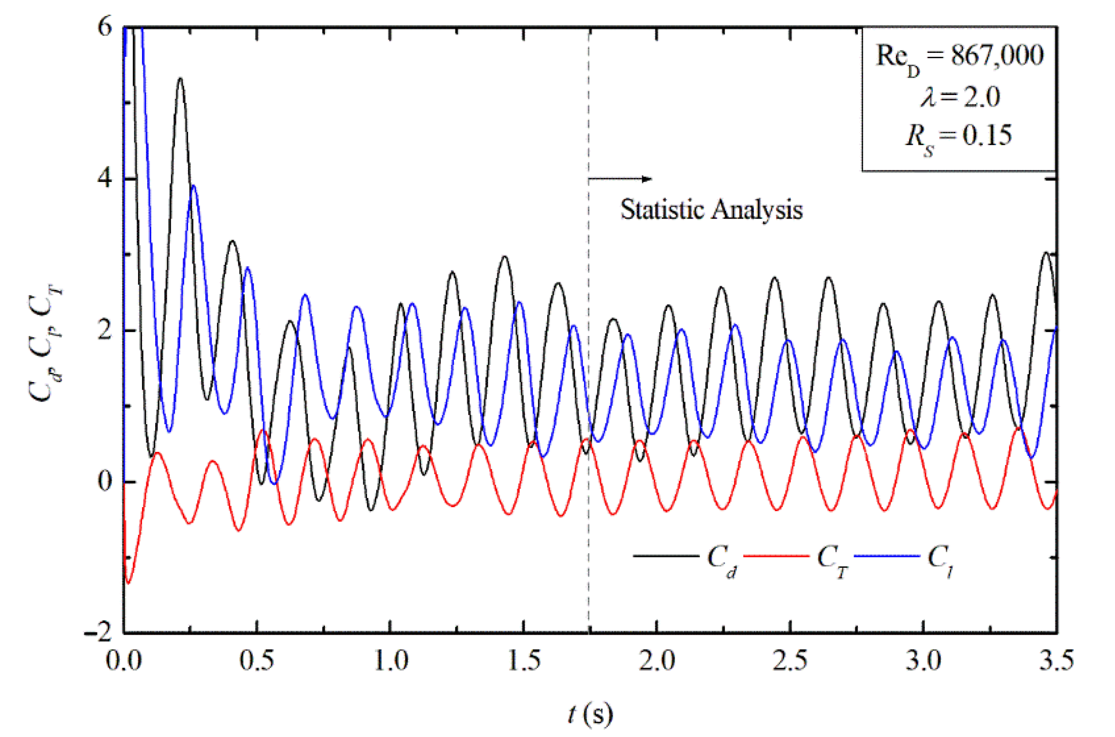
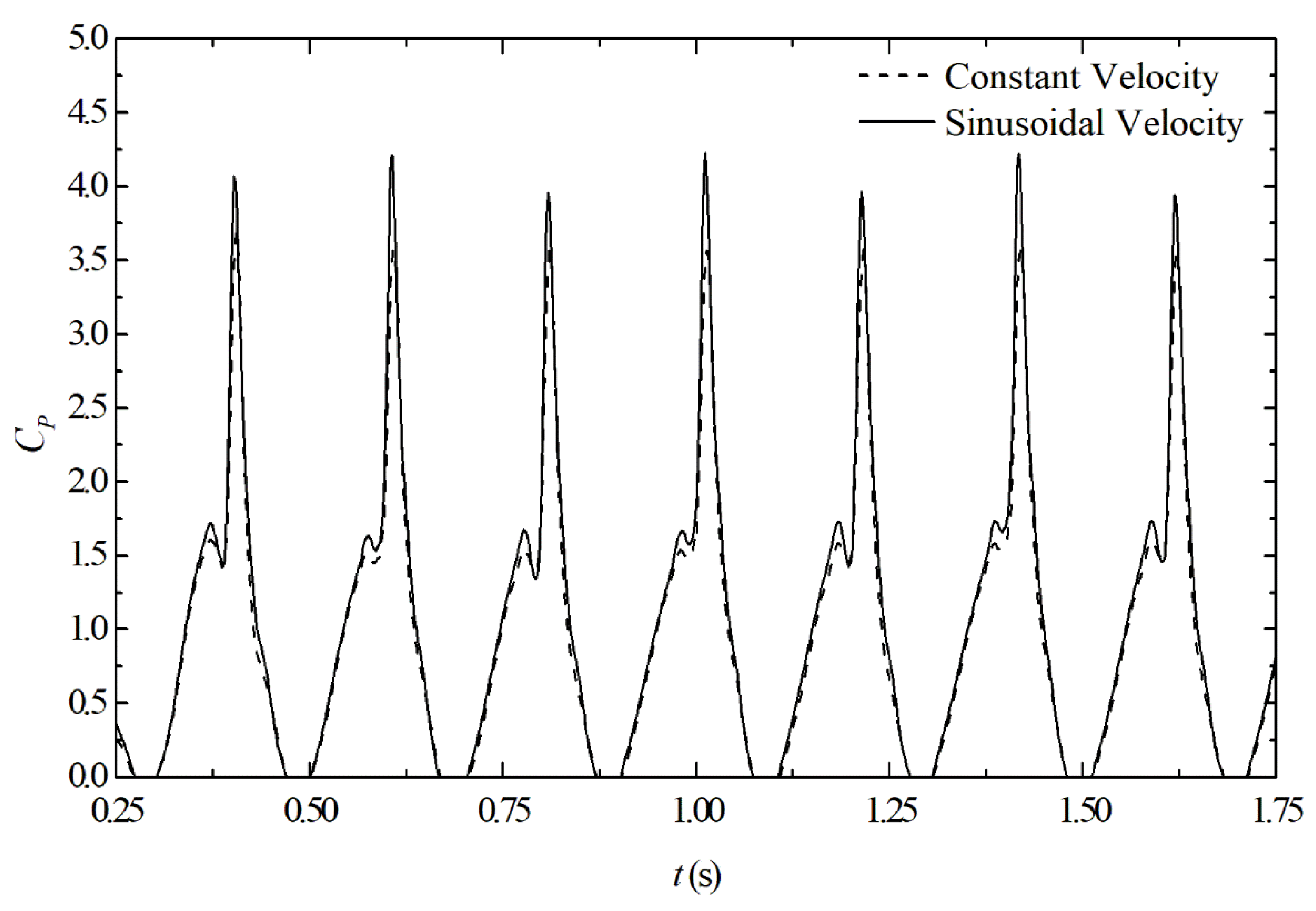
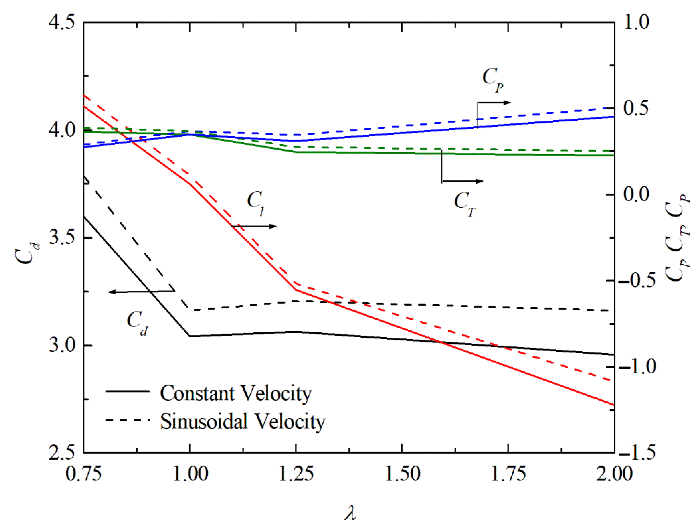
4.1. Verification/Validation of the Computational Model (Case 1)

Figure 4 illustrates the instantaneous drag, lift, and moment coefficients as a function of time for Case 1 with Re_D = 867,000, λ = 2.0, and R_S = 0.15. For the first instants of time, mainly for t ≤ 0.5 s, the coefficients had a strong variation due to the incidence of the fluid flow and the imposition of angular velocity in the rotational domain region. Therefore, the present model must be used to predict power in the turbine when the flow is stabilized, and the first cycles of rotation of the turbine were disregarded for the analysis of coefficients and power. Here, for the computation of time-averaged parameters, only the results in the range of time 1.75 s ≤ t ≤ 3.5 s were used. Despite the complexity of the fluid flow, the results also demonstrated a regular oscillation in the magnitudes of C_d, C_l, and C_T, which had similar behavior to that previously obtained in Akwa et al. [49]. Moreover, the crest and cave magnitudes were also similar, showing the generation of regular wakes of vortices behind the turbine.

Figure 5 shows the comparison of power coefficients (C_P) as a function of the tip speed ratio (λ) obtained with the present computational model and the numerical predictions of Akwa et al. [49] obtained with other commercial code (Star-CCM+) also based on the FVM and the experimental results of Blackwell et al. [48]. The results predicted with the present method are in close agreement with those previously obtained in the literature, verifying and validating the method used here. Even for λ = 1.00 and 2.00, where the highest differences between the present results and the experimental ones were obtained, the deviations were lower than the uncertainty of the experiment. The results indicated that the highest magnitudes of $\overline{C_P}$ were reached at the lowest values of λ. With the increase in λ, the magnitude of $\overline{C_P}$ had a slight decrease in the range 1.00 ≤ λ ≤ 1.25 and a step decrease for λ ≥ 1.25. For λ = 2.00, negative magnitudes of $\overline{C_P}$ were obtained, indicating that the device supplies energy for the fluid flow and not the contrary.

Figure 6 and Figure 7 illustrate the velocity and pressure fields, respectively, for Case 1 with Re_D = 867,000 and λ = 1.25 for five different instants of time: (a) t = 0.0 s, (b) t = 0.53 s, (c) t = 1.05 s, (d) t = 1.58 s, and (e) t = 2.10 s, which represent different angular positions of the Savonius rotor. For the initial time step, in Figure 6a and Figure 7a, the velocity and pressure fields noticed were generated by the imposition of angular velocity in the rotational domain by the computational model. This behavior does not represent the real condition of fluid flow over the turbine since the turbine should not be in motion before the incidence of the fluid flow. Therefore, the present computational method must be used when the flow is stabilized, which happens a few cycles later at the beginning of the fluid flow (as shown in Figure 4 for monitoring the coefficients). As the time advances, mainly for t > 1.0 s, Figure 6c–e and Figure 7c–e show an increase in the pressure field magnitude on the concave side of the advancement blade and a pressure drop as a consequence, being the main reason for the pressure drag force that drives the turbine. The results also show the fluid flowing in the region between the two blades. The results also show the generation of wakes behind the rotor and vortices generated in the tip region of the blade. It is also worth mentioning that the behavior found here is similar to that described in previous literature, e.g., in Prasad et al. [45] and Blackwell et al. [49].

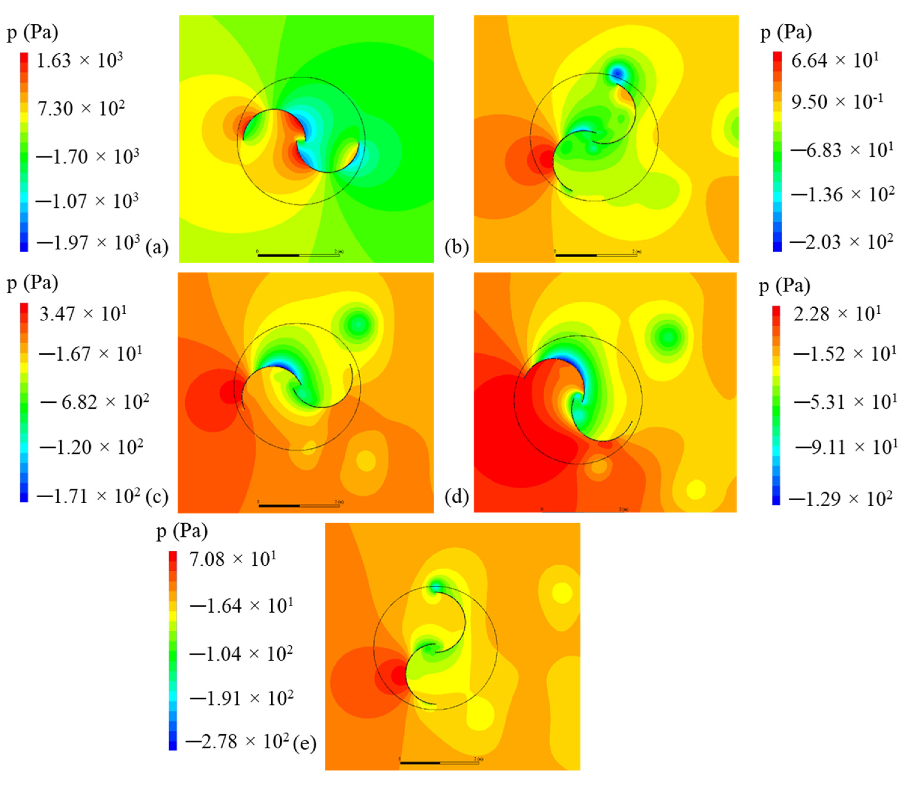
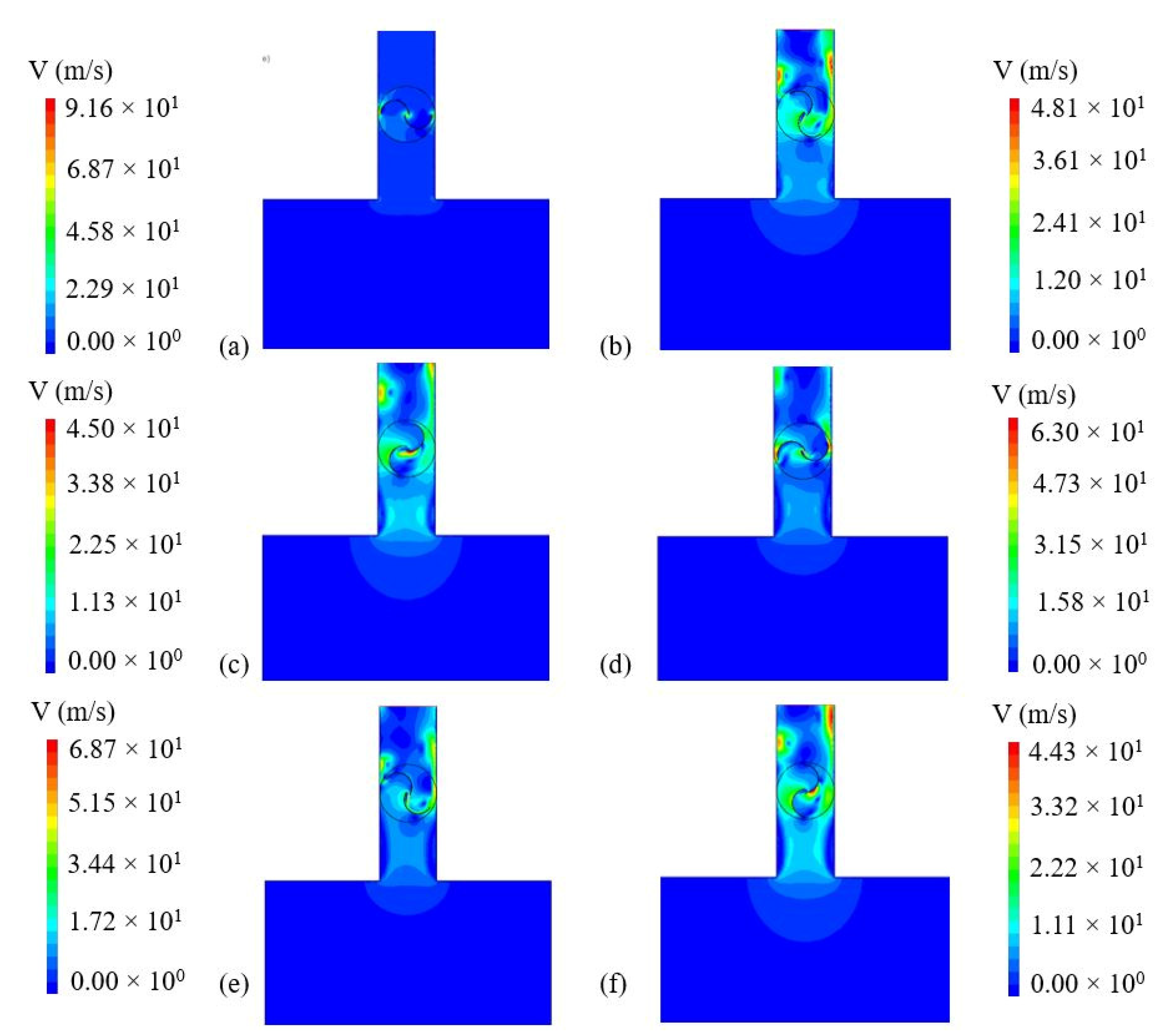
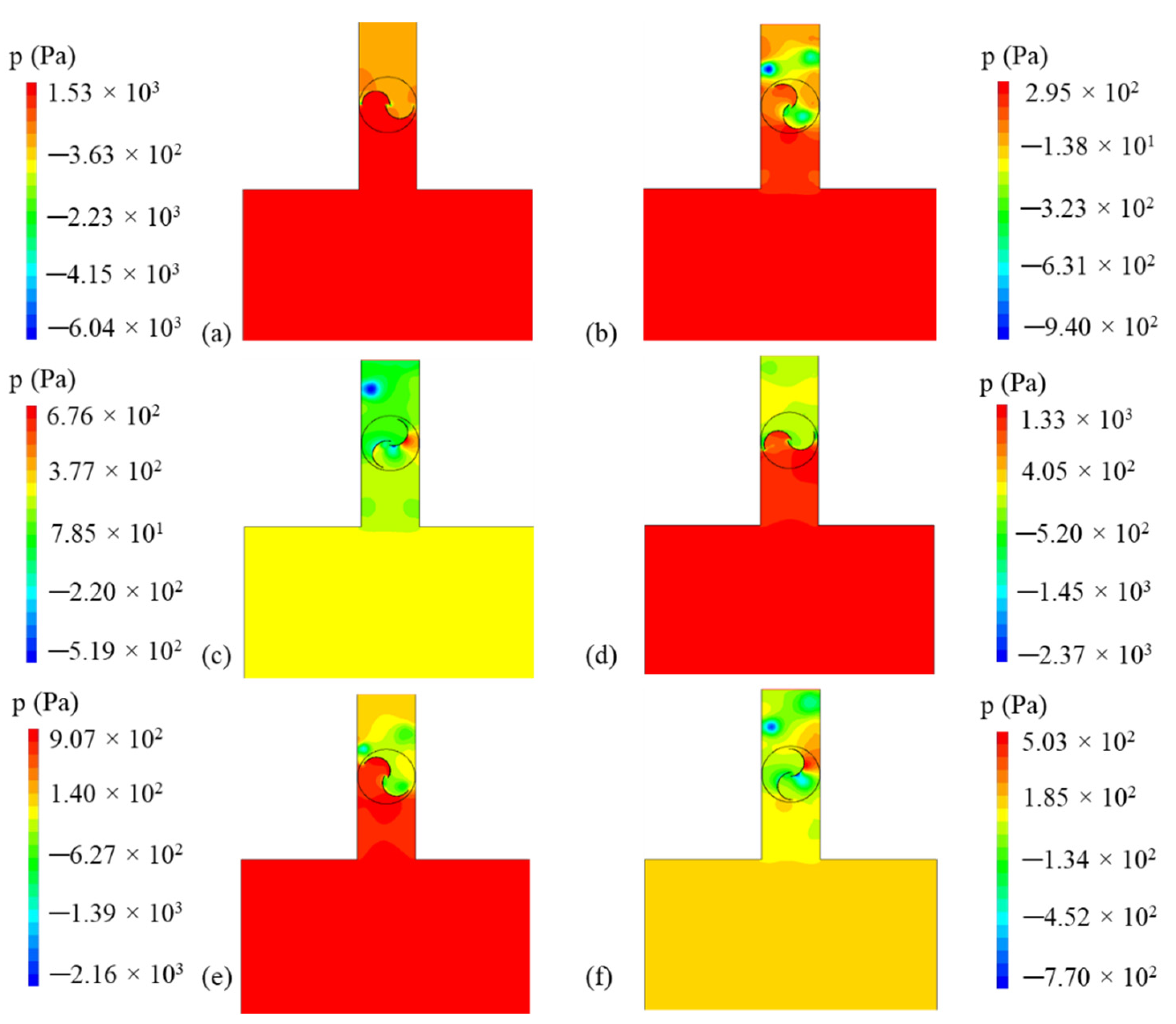
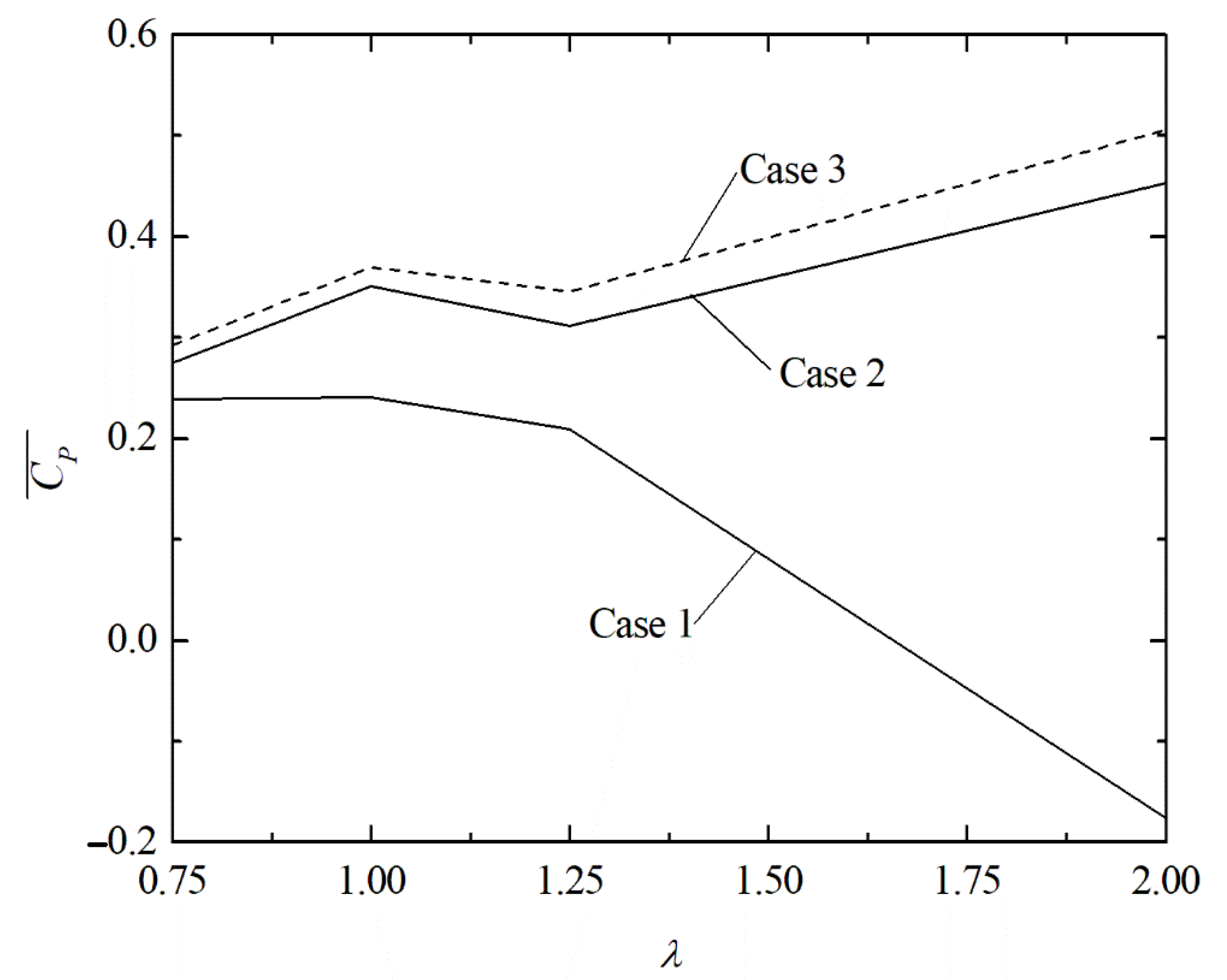
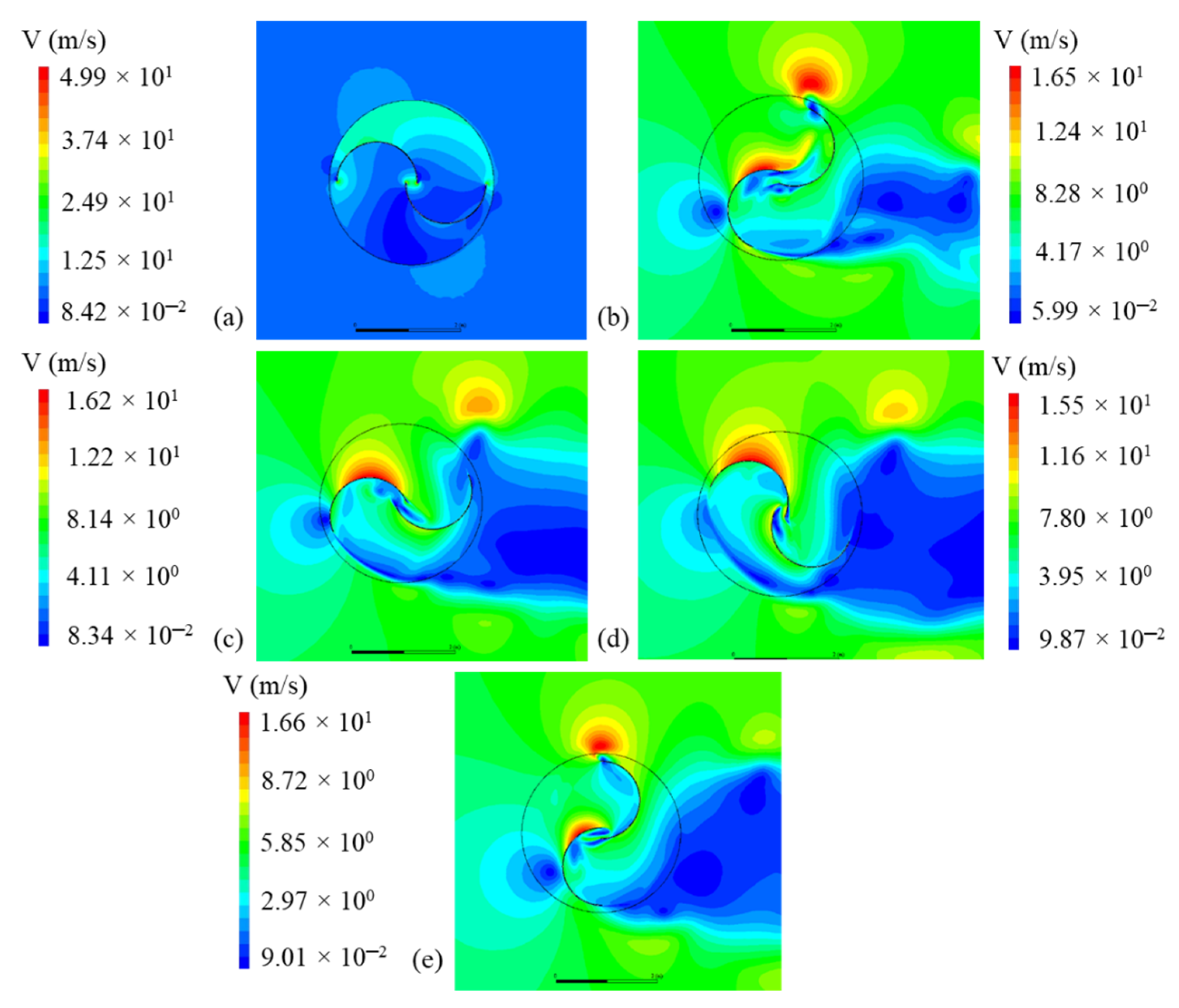
4.2. The Results of the Savonius Turbine Inserted in an OWC Domain (Case 2 and Case 3)

For the turbulent air flow in the enclosure domain, the instantaneous aerodynamic coefficients (C_d, C_l, and C_T) were obtained as a function of time to better understand the behavior of the turbine in an OWC domain. Figure 8 depicts the coefficients for the flow with Re_D = 867,000, λ = 2.0, and R_S = 0.15 for a constant imposed velocity at the inlet (Case 2). In general, the results show an average increase in C_d (black line) for all instants of time compared to the free turbine simulations (Case 1) due to the insertion of the turbine in the enclosure domain. The increase in the drag coefficient (C_d) also led to an augmentation of the moment coefficient (C_T) represented in red color in a similar form reached for the C_d, while the lift coefficient (C_l) did not suffer important modifications in its mean magnitude. The results also indicate that the transient behavior of the coefficients was strongly modified compared to Case 1, showing C_d and C_l with sharp peaks and smooth troughs, i.e., each cycle did not behave in a sinusoidal form as noticed in Figure 4 for the free turbine configuration. It is worth mentioning that, for other magnitudes of λ, similar behavior for the instantaneous coefficients was obtained. Therefore, for the sake of brevity, the instantaneous coefficients for other magnitudes of λ are not presented.

As previously mentioned, the air flow in the OWC chamber is subjected to the piston-type oscillatory motion of the water column (hydropneumatic chamber). In order to simulate this effect, the results of instantaneous power coefficient obtained for Case 3 and Case 2, considering the same conditions (Re_D = 867,000, λ = 2.0, and R_S = 0.15), are presented in Figure 9. It is important to reinforce that, for prediction of C_P for Case 2 and Case 3, Equation (6) was used instead of Equation (5), and the time-averaged magnitudes were predicted with Equation (7). The results reveal a strong similarity between the instantaneous C_P for both cases, indicating that the imposition of sinusoidal velocity at the inlet of the domain did not have a significant influence over the pattern of the C_P investigated here, which is not intuitively expected since the mean imposed momentum decreased for Case 3 in comparison with Case 2. The results also demonstrate a slight increase in the power coefficients when the sinusoidal velocity was imposed, with a difference of nearly 9.0% on average. Possible explanations for the behavior found here include the synchronization of velocity augmentation with the rotation of the turbine and the imposition of the rotational domain, as well as the acceleration of the fluid caused by the variation of the imposed velocity at the inlet for Case 3, which did not happen for Case 2. The magnitude of the imposed mean velocity at the inlet of Case 2 and Case 3 and acceleration at the inlet for Case 3 are illustrated in Figure 10 to make this visualization easy. It is worth mentioning that, despite different imposed inlet velocities, the transient fields of velocity and pressure had only slight differences. Future investigations should be performed with other magnitudes of amplitude and periods of imposed velocity to corroborate this hypothesis and the development of other models where the inertia moment of the turbine is taken into account.

Figure 11 and Figure 12 illustrate the velocity and pressure fields, respectively, for the simulation of Case 3 with Re_D = 867,000, λ = 2.0, and R_S = 0.15 for six different time steps: (a) t = 0.0 s, (b) t = 0.26 s, (c) t = 0.53 s, (d) t = 0.79 s, (e) t = 1.05 s, and (f) t = 1.31 s. As the behaviors of Case 3 and Case 2 were almost the same, only the fields for one of the cases are illustrated. As previously mentioned, for the free turbine case (see Figure 6 and Figure 7), the initial time steps should be disregarded due to the artificial imposition of the angular velocity in the turbine region. In spite of that, when the flow was stabilized, the model properly represented the physical problem. In turn, one can note in Figure 11 and Figure 12 an increase in the pressure difference between the concave and convex sides of the advancement blade for Case 2 and Case 3 compared to Case 1, which explains the augmentation of the pressure drag in comparison with Case 1.

Moreover, the pressure difference between the upstream and downstream regions of the turbine was also augmented. This influence over the water oscillation was not investigated, but the results pointed out that this aspect is worth investigation when the turbine is taken into account in the problem in order to avoid the restriction of the water column, mainly when coupling with a wave channel is performed. The results also indicated the variation of the pressure magnitude in the chamber for different instants of time, explaining the non-symmetric differences between the peaks and troughs with respect to the mean magnitudes of the coefficients. The momentum of the fluid flow intensified due to the insertion of the turbine in the enclosure domain. Moreover, the wakes generated in the turbine and secondary vortices in the tip of the blades could not be spread in the spanwise direction of the main flow due to the limitation imposed by the air duct walls. Therefore, as expected, the insertion of the turbine in the enclosure domain affected the fluid dynamic behavior of the flow considerably.

To summarize, Figure 13 shows the effect of λ on the time-averaged magnitudes of $\overline{C_d},\overline{C_l},\overline{C_T}$ and $\overline{C_P}$ for Case 2 and Case 3, and Figure 14 illustrates the same effect considering only $\overline{C_P}$ for Case 1, Case 2, and Case 3. The results indicate that the differences between the values of the aerodynamic and power coefficients obtained for Case 2 and Case 3 were not significant, with the highest difference being lower than 10.0%. The effect of λ on the coefficients was also similar for both cases. Concerning the magnitude of $\overline{C_d}$, it decreased in the range 0.75 ≤ λ ≤ 1.00, and after this point, the magnitude was almost constant. The $\overline{C_l}$ and $\overline{C_T}$ magnitudes decreased with the increase in λ. However, for $\overline{C_T}$ the decrease was more significant only in the range 1.00 ≤ λ ≤ 1.25, being almost constant in other intervals of λ. For the $\overline{C_P}$, there was an increase with the augmentation of λ. For Case 3, for example, the magnitude increased from $\overline{C_P}$ = 0.2922 when λ = 0.75 to $\overline{C_P}$ = 0.5054 when λ = 2.0. Figure 14 indicates that in the region 0.75 ≤ λ ≤ 1.25, a similar trend of $\overline{C_P}$ was noticed when Case 1 and the enclosure cases (Case 2 and Case 3) were compared. However, for λ = 2.0, contrary to the behavior noticed for Case 1, Case 2 and Case 3 did not have a reduction of $\overline{C_P}$ for the highest magnitude of λ investigated. Therefore, the results indicated that changes in the domain where the turbine is placed are important to define its application range and the effect of λ over the problem performance. Further studies should be performed to define the range of application of λ for the enclosure domain.

5. Conclusions

The present work developed a computational model to investigate turbulent flows in enclosure domains with an inserted Savonius turbine simulating the air flow in an OWC/WEC device. Initially, a free turbine configuration (Case 1) was investigated in order to perform the verification/validation of the present method. Then, two different study cases were investigated (Case 2 and Case 3) with constant and sinusoidal velocity imposed at the domain inlet. For all cases, Re_D = 867,000, R_S = 0.15, and four different magnitudes of λ were studied (λ = 0.75, 1.00, 1.25, and 2.00). For the simulation of incompressible, two-dimensional, transient, and turbulent flows, the time-averaged equations of mass conservation, the balance of momentum, and transport equations of the k–ω SST model were solved with the FVM.

The proposed computational model was verified and validated using a comparison of C_P with the numerical and experimental results of the literature [48,49], reproducing the effect of λ on $\overline{C_P}$ for the turbulent flow over a free Savonius turbine. Moreover, the velocity and pressure fields demonstrated that the driven force of the Savonius turbine was dominated by the pressure difference between the concave and convex sides of the advancement blade, which the present model adequately predicted.

After the verification/validation of the computational model, new recommendations were reached for the turbulent flows over the Savonius turbine inserted in the enclosure domain representing an OWC. The results demonstrated that the new configuration had a strong influence over the behavior and magnitudes of the instantaneous coefficients such as C_d and C_T, also affecting the instantaneous values of C_P. For the investigated values of λ, the results indicated that the insertion of a turbine in the enclosure domain led to an overall augmentation of $\overline{C_P}$ for all values of λ. In addition, the effect of λ on $\overline{C_d},\overline{C_l},\overline{C_T}$, and $\overline{C_P}$ was strongly affected by the domain change, indicating that the geometric configuration can be important to define the range of applicability of the turbine and the design of the PTO in the OWC device. The comparison between the imposition of sinusoidal velocity (Case 3) and constant velocity (Case 2) at the domain inlet led to similar performance and aerodynamic coefficients. It is important to highlight that due to the two-dimensional approach, some characteristics of the air flow phenomenology through the Savonious turbine cannot be completely revealed from the obtained results, being a limitation of the proposed computational model.

Future investigations should be performed considering a model where the inertia moment is taken into account to verify if this behavior continues to be observed. It is recommended to investigate other parameters, such as the effect of the overlap and spacing between the blades (s and a) and other tip speed ratios (λ) on the aerodynamic and performance of the OWC and the imposition of irregular velocity variation to represent the real sea state movement. It is also recommended to investigate the coupling between the present model and the wave channel for adequate simulation of the interaction between the oncoming waves, the structure of the device, and air flow over the turbine inserted in the OWC air duct.

References

1. International Energy Agency (IEA). World Energy Outlook 2019; International Energy Agency: Paris, France, 2019. [Google Scholar]
2. Jenniches, S. Assessing the regional economic impacts of renewable energy sources—A literature review. Renew. Sustain. Energy Rev. 2018, 93, 35–51. [Google Scholar] [CrossRef]
3. Cheng, M.; Zhu, Y. The state of the art of wind energy conversion systems and technologies: A review. Energy Convers. Manag. 2014, 88, 332–347. [Google Scholar] [CrossRef]
4. Olabi, A.G.; Wilberforce, T.; Elsaid, K.; Salameh, T.; Sayed, E.T.; Husain, K.S.; Abdelkareem, M.A. Selection Guidelines for Wind Energy Technologies. Energies 2021, 14, 3244. [Google Scholar] [CrossRef]
5. Kumar, K.R.; Chaitanya, N.V.V.K.; Kumar, N.S. Solar thermal energy technologies and its applications for process heating and power generation—A review. J. Clean. Prod. 2021, 282, 125296. [Google Scholar] [CrossRef]
6. Seme, S.; Štumberger, B.; Hadžiselimović, M.; Sredenšek, K. Solar Photovoltaic Tracking Systems for Electricity Generation: A Review. Energies 2020, 13, 4224. [Google Scholar] [CrossRef]
7. Nunes, B.R.; Rodrigues, M.K.; Rocha, L.A.O.; Labat, M.; Lorente, S.; Dos Santos, E.D.; Isoldi, L.A.; Biserni, C. Numerical-analytical study of earth-air heat exchangers with complex geometries guided by constructal design. Int. J. Energy Res. 2021, 45, 20970–20987. [Google Scholar] [CrossRef]
8. Khan, N.; Kalair, A.; Abas, N.; Haider, A. Review of ocean tidal, wave and thermal energy technologies. Renew. Sustain. Energy Rev. 2017, 72, 590–604. [Google Scholar] [CrossRef]
9. Melikoglu, M. Current status and future of ocean energy sources: A global review. Ocean Eng. 2018, 148, 563–573. [Google Scholar] [CrossRef]
10. Curto, D.; Franzitta, V.; Guercio, A. Sea Wave Energy. A Review of the Current Technologies and Perspectives. Energies 2021, 14, 6604. [Google Scholar] [CrossRef]
11. Chen, L.; Li, W.; Li, J.; Fu, Q.; Wang, T. Evolution Trend Research of Global Ocean Power Generation Based on a 45-Year Scientometric Analysis. J. Mar. Sci. Eng. 2021, 9, 218. [Google Scholar] [CrossRef]
12. Falcão, A.F.D.O. Wave Energy Utilization: A Review of the Technologies. Renew. Sustain. Energy Rev. 2010, 14, 899–918. [Google Scholar] [CrossRef]
13. Zabihian, F.; Fung, A.S. Review of Marine Renewable Energies: Case Study of Iran. Renew. Sustain. Energy Rev. 2011, 15, 2461–2474. [Google Scholar] [CrossRef]
14. López, I.; Andreu, J.; Ceballos, S.; De Alegría, I.M.; Kortabarria, I. Review of wave energy technologies and the necessary power-equipment. Renew. Sustain. Energy Rev. 2013, 27, 413–434. [Google Scholar] [CrossRef]
15. Liu, W.; Xu, X.; Chen, F.; Liu, Y.; Li, S.; Liu, L.; Chen, Y. A Review of Research on the Closed Thermodynamic Cycles of Ocean Thermal Energy Conversion. Renew. Sustain. Energy Rev. 2020, 119, 109581. [Google Scholar] [CrossRef]
16. Temiz, I.; Ekweoba, C.; Thomas, S.; Kramer, M.; Savin, A. Wave Absorber Ballast Optimization based on the Analytical Model for a Pitching Wave Energy Converter. Ocean Eng. 2021, 240, 109906. [Google Scholar] [CrossRef]
17. Müller, G.; Whittaker, T.J.T. Field measurements of breaking wave loads on a shoreline wave power station. Proc. ICE Water Marit. Energy 1995, 112, 187–197. [Google Scholar] [CrossRef]
18. Müller, G.; Whittaker, T.J.T. An evaluation of design wave impact pressures. J. Waterw. Port Coast. Ocean Eng. 1996, 122, 55–58. [Google Scholar] [CrossRef]
19. Patterson, C.; Dunsire, R.; Hillier, S. Development of wave energy breakwater at Siadar, Isle of Lewis. In Proceedings of the ICE Conference Coasts, Marine Structures & Breakwaters, Edinburgh, UK, 16–18 September 2009; pp. 738–749. [Google Scholar] [CrossRef]
20. Bryden, I.G. Progress towards a viable UK marine renewable energy. In Proceedings of the ICE Conference Coasts, Marine Structures & Breakwaters, Edinburgh, UK; 2009; pp. 2–13. [Google Scholar] [CrossRef]
21. Torre-Enciso, Y.; Ortubia, I.; López de Aguileta, L.I.; Marqués. Mutriku Wave Power Plant: From the thinking out to the reality. In Proceedings of the 8th European Wave and Tidal Energy Conference, Uppsala, Sweden, 7–10 September 2009; pp. 319–329. [Google Scholar]
22. Torre-Enciso, Y.; Marqués, J.; López de Aguileta, L.I. Mutriku. Lessons learnt. In Proceedings of the 3rd International Conference on Ocean Energy, Bilbao, Spain, 6–8 October 2010; pp. 1–6. [Google Scholar]
23. Dizadji, N.; Sajadian, S.E. Modeling and Optimization of the Chamber of OWC System. Energy 2011, 36, 2360–2366. [Google Scholar] [CrossRef]
24. Mahnamfar, F.; Altunkaynak, A. OWC-Type Wave Chamber Optimization under Series of Regular Waves. Arab. J. Sci. Eng. 2016, 41, 1543–1549. [Google Scholar] [CrossRef]
25. Viviano, A.; Naty, S.; Foti, E.; Bruce, T.; Allsop, W.; Vicinanza, D. Large-Scale Experiments on the Behaviour of Generalised Oscillating Water Column under Random Waves. Renew. Energy 2016, 99, 875–887. [Google Scholar] [CrossRef] [Green Version]
26. Gadelho, J.F.M.; Rezanejad, K.; Xu, S.; Hinostroza, M.; Soares, C.G. Experimental study on the motions of a dual chamber floating oscillating water column device. Renew. Energy 2021, 170, 1257–1274. [Google Scholar] [CrossRef]
27. Rezanejad, K.; Gadelho, J.F.M.; Xu, S.; Soares, C.G. Experimental investigation on the hydrodynamic performance of a new type floating Oscillating Water Column device with dual-chambers. Ocean Eng. 2021, 234, 109307. [Google Scholar] [CrossRef]
28. Maciel, R.P.; Fragassa, C.; Machado, B.N.; Rocha, L.A.O.; Dos Santos, E.D.; Gomes, M.N.; Isoldi, L.A. Verification and Validation of a Methodology to Numerically Generate Waves Using Transient Discrete Data as Prescribed Velocity Boundary Condition. J. Mar. Sci. Eng. 2021, 9, 896. [Google Scholar] [CrossRef]
29. Conde, J.M.; Gato, L.M.C. Numerical study of the air-flow in an oscillating water column wave energy converter. Renew. Energy 2008, 33, 2637–2644. [Google Scholar] [CrossRef]
30. Liu, Z.; Hyun, B.; Hong, K. Numerical study of air chamber for oscillating water column wave energy convertor. China Ocean Eng. 2011, 25, 169–178. [Google Scholar] [CrossRef]
31. Gomes, M.d.N.; Dos Santos, E.D.; Isoldi, L.A.; Rocha, L.A.O. Numerical Analysis including Pressure Drop in Oscillating Water Column Device. Open Eng. 2015, 5, 229–237. [Google Scholar] [CrossRef] [Green Version]
32. Elhanafi, A.; Macfarlane, G.; Fleming, A.; Leong, Z. Experimental and numerical investigations on the hydrodynamic performance of a floating–moored oscillating water column wave energy converter. Appl. Energy 2017, 205, 369–390. [Google Scholar] [CrossRef]
33. Moñino, A.; Medina-López, E.; Clavero, M.; Benslimane, S. Numerical Simulation of a Simple OWC Problem for Turbine Performance. Int. J. Mar. Energy 2017, 20, 17–32. [Google Scholar] [CrossRef]
34. Mahnamfar, F.; Altunkaynak, A. Comparison of Numerical and Experimental Analyses for Optimizing the Geometry of OWC Systems. Ocean Eng. 2017, 130, 10–24. [Google Scholar] [CrossRef]
35. Torres, F.R.; Teixeira, P.R.F.; Didier, E. A Methodology to Determine the Optimal Size of a Wells Turbine in an Oscillating Water Column Device by Using Coupled Hydro-Aerodynamic Models. Renew. Energy 2018, 121, 9–18. [Google Scholar] [CrossRef]
36. Gonçalves, R.A.A.C.; Teixeira, P.R.F.; Didier, E.; Torres, F.R. Numerical analysis of the influence of air compressibility effects on an oscillating water column wave energy converter chamber. Renew. Energy 2020, 153, 1183–1193. [Google Scholar] [CrossRef]
37. Gomes, M.N.; Lorenzini, G.; Rocha, L.A.O.; Dos Santos, E.D.; Isoldi, L.A. Constructal Design Applied to the Geometric Evaluation of an Oscillating Water Column Wave Energy Converter Considering Different Real Scale Wave Periods. J. Eng. Thermophys. 2018, 27, 173–190. [Google Scholar] [CrossRef]
38. Kharati-Koopaee, M.; Fathi-Kelestani, A. Assessment of oscillating water column performance: Influence of wave steepness at various chamber lengths and bottom slopes. Renew. Energy 2020, 147, 1595–1608. [Google Scholar] [CrossRef]
39. Letzow, M.; Lorenzini, G.; Barbosa, D.V.E.; Hübner, R.G.; Rocha, L.A.O.; Gomes, M.N.; Isoldi, L.A.; Dos Santos, E.D. Numerical Analysis of the Influence of Geometry on a Large Scale Onshore Oscillating Water Column Device with Associated Seabed Ramp. Int. J. Des. Nat. Ecodyn. 2020, 15, 873–884. [Google Scholar] [CrossRef]
40. Lima, Y.T.B.; Gomes, M.N.; Isoldi, L.A.; Dos Santos, E.D.; Lorenzini, G.; Rocha, L.A.O. Geometric Analysis through the Constructal Design of a Sea Wave Energy Converter with Several Coupled Hydropneumatic Chambers Considering the Oscillating Water Column Operating Principle. Appl. Sci. 2021, 11, 8630. [Google Scholar] [CrossRef]
41. Gomes, M.D.N.; Salvador, H.; Magno, F.; Rodrigues, A.A.; Santos, E.D.; Isoldi, L.A.; Rocha, L.A.O. Constructal Design Applied to Geometric Shapes Analysis of Wave Energy Converters. Defect Diffus. Forum 2021, 407, 147–160. [Google Scholar] [CrossRef]
42. Lisboa, R.C.; Teixeira, P.R.F.; Torres, F.R.; Didier, E. Numerical Evaluation of the Power Output of an Oscillating Water Column Wave Energy Converter Installed in the Southern Brazilian Coast. Energy 2018, 162, 1115–1124. [Google Scholar] [CrossRef]
43. Machado, B.N.; Oleinik, P.H.; Kirinus, E.P.; Dos Santos, E.D.; Rocha, L.A.O.; Gomes, M.N.; Conde, J.M.P.; Isoldi, L.A. WaveMIMO Methodology: Numerical Wave Generation of a Realistic Sea State. J. Appl. Comput. Mech. 2021, 7, 2129–2148. [Google Scholar] [CrossRef]
44. Brito-Melo, A.; Gato, L.M.C.; Sarmento, A.J.N.A. Analysis of Wells Turbine Design Parameters by Numerical Simulation of the OWC Performance. Ocean Eng. 2002, 29, 1463–1477. [Google Scholar] [CrossRef]
45. Rodríguez, L.; Pereiras, B.; García-Diaz, M.; Fernandez-Oro, J.; Castro, F. Flow pattern analysis of an outflow radial turbine for twin-turbines-OWC wave energy converters. Energy 2020, 211, 118584. [Google Scholar] [CrossRef]
46. Prasad, D.D.; Ahmed, M.R.; Lee, Y.-H. Studies on the Performance of Savonius Rotors in a Numerical Wave Tank. Ocean Eng. 2018, 158, 29–37. [Google Scholar] [CrossRef]
47. Liu, Z.; Xu, C.; Kim, K.; Choi, J.; Hyun, B. An integrated numerical model for the chamber-turbine system of an oscillating water column wave energy converter. Renew. Sust. Energy Rev. 2021, 149, 111350. [Google Scholar] [CrossRef]
48. Blackwell, B.F.; Sheldahl, R.E.; Feltz, L.V. Wind Tunnel Performance Data for Two-and Three-Buckets Savonius Rotors; Final Report SAND76-0131; Sandia Laboratories: Albuquerque, NM, USA, 1977. [Google Scholar]
49. Akwa, J.V.; Silva Júnior, G.A.; Petry, A.P. Discussion on the Verification of the Overlap Ratio Influence on Performance Coefficients of a Savonius Wind Rotor using Computational Fluid Dynamics. Renew. Energy 2021, 38, 141–149. [Google Scholar] [CrossRef]
50. Schlichting, H.; Gersten, K. Boundary-Layer Theory, 8th ed.; Springer: Berlin/Heidelberg, Germany, 2000. [Google Scholar]
51. Wilcox, D.C. Turbulence Modeling for CFD, 3rd ed.; DWC Industries: La Cañada Flintridge, CA, USA, 2006. [Google Scholar]
52. Menter, F.R. Zonal Two Equation j–x Turbulence Models for Aerodynamic Flows. In Proceedings of the AIAA 24th Fluid Dynamics Conference, Orlando, FL, USA, 6–9 July 1993. AIAA 93-2906. [Google Scholar]
53. Menter, F.R.; Kuntz, M.; Langtry, R. Ten Years of Industrial Experience with the SST Turbulence Model. In Turbulence, Heat and Mass Transfer; Hanjalić, K., Nagano, Y., Tummers, M., Eds.; Begell House: Danbury, CT, USA, 2003; Volume 4, pp. 625–632. [Google Scholar]
54. Versteeg, H.K.; Malalasekera, W. An Introduction to Computational Fluid Dynamics—The Finite Volume Method, 2nd ed.; Longman: London, UK, 2007. [Google Scholar]
55. Patankar, S.V. Numerical Heat Transfer and Fluid Flow; McGraw-Hill: New York, NY, USA, 1980. [Google Scholar]
56. ANSYS Inc. Ansys Fluent Theory Guide; ANSYS Inc.: Cannonsburg, PA, USA, 2013. [Google Scholar]
57. Khaligh, A.; Onar, O.C. Energy Harvesting—Solar, Wind and Ocean Energy Conversion Systems; CRC Press: Boca Raton, FL, USA; Taylor and Francis: Abingdon, UK, 2010. [Google Scholar]
58. Geuzaine, C.; Remacle, J.-F. Gmsh: A 3-D Finite Element Mesh Generator with Built-in Pre and Post-Processing Facilities. Int. J. Numer. Meth. Eng. 2009, 11, 1309–1331. [Google Scholar] [CrossRef]
Figure 1. Schematic representation of the computational domain of turbulent air flow over a free Savonius turbine used for verification/validation of the present numerical model (Case 1).
Jmse 10 00079 g001
Figure 2. Schematic representation of Case 2 and Case 3 that simulate the OWC with a Savonius turbine.
Jmse 10 00079 g002
Figure 3. Employed mesh for the studied cases: (a) turbine in the open channel (Case 1), (b) turbine in an OWC chamber domain (Case 2 and Case 3), (c) detail of grid refinement the surfaces of the blades.
Jmse 10 00079 g003
Figure 4. Transient coefficients of the lift (Cl), drag (Cd), and torque (CT) for the free turbine case with ReD = 867,000, Rs = 0.15, and λ = 2.0.
Jmse 10 00079 g004
Figure 5. Comparison between the power coefficient (CP) as a function of λ obtained in the present work and that from the literature [48,49].
Jmse 10 00079 g005
Figure 6. Velocity fields around the free turbine (Case 1) with ReD = 867,000 and λ = 1.25: (a) t = 0.0 s, (b) t = 0.53 s, (c) t = 1.05 s, (d) t = 1.58 s, and (e) t = 2.10 s.
Jmse 10 00079 g006
Figure 7. Pressure fields around the free turbine (Case 1) with ReD = 867,000 and λ = 1.25: (a) t = 0.0 s, (b) t = 0.53 s, (c) t = 1.05 s, (d) t = 1.58 s, and (e) t = 2.10 s.
Jmse 10 00079 g007
Figure 8. Instantaneous coefficients of the drag (Cd), lift (Cl), and moment (CT) for the case of OWC with constant imposed velocity at the inlet (Case 2) with ReD = 867,000, λ = 2.0, and RS = 0.15.
Jmse 10 00079 g008
Figure 9. Effect of imposed velocity at the inlet of the OWC domain over the instantaneous power coefficient in the Savonius turbine, considering ReD = 867,000, λ = 2.0, and RS = 0.15.
Jmse 10 00079 g009
Figure 10. Magnitude of the imposed velocity at the inlet of the OWC domain for Case 2 and Case 3 and acceleration of the fluid at the inlet of the domain for Case 3.
Jmse 10 00079 g010
Figure 11. Velocity fields for the OWC case with sinusoidal velocity at the inlet for different instants of time for the case with ReD = 867,000, λ = 2.0, and RS = 0.15: (a) t = 0.0 s, (b) t = 0.26 s, (c) t = 0.53 s, (d) t = 0.79 s, (e) t = 1.05 s, and (f) t = 1.31 s.
Jmse 10 00079 g011
Figure 12. Pressure fields for the OWC case with sinusoidal velocity at the inlet for different instants of time for the case with ReD = 867,000, λ = 2.0, and RS = 0.15: (a) t = 0.0 s, (b) t = 0.26 s, (c) t = 0.53 s, (d) t = 0.79 s, (e) t = 1.05 s, and (f) t = 1.31 s.
Jmse 10 00079 g012
Figure 13. Averaged coefficients as a function of λ for the cases of OWC with constant- and sinusoidal-imposed velocity.
Jmse 10 00079 g013
Figure 14. Power coefficients as a function of the tip speed ratio for the three studied cases (Case 1, Case 2, and Case 3).
Jmse 10 00079 g014