
Implementation of the IMO Second Generation Intact Stability Guidelines

Abstract
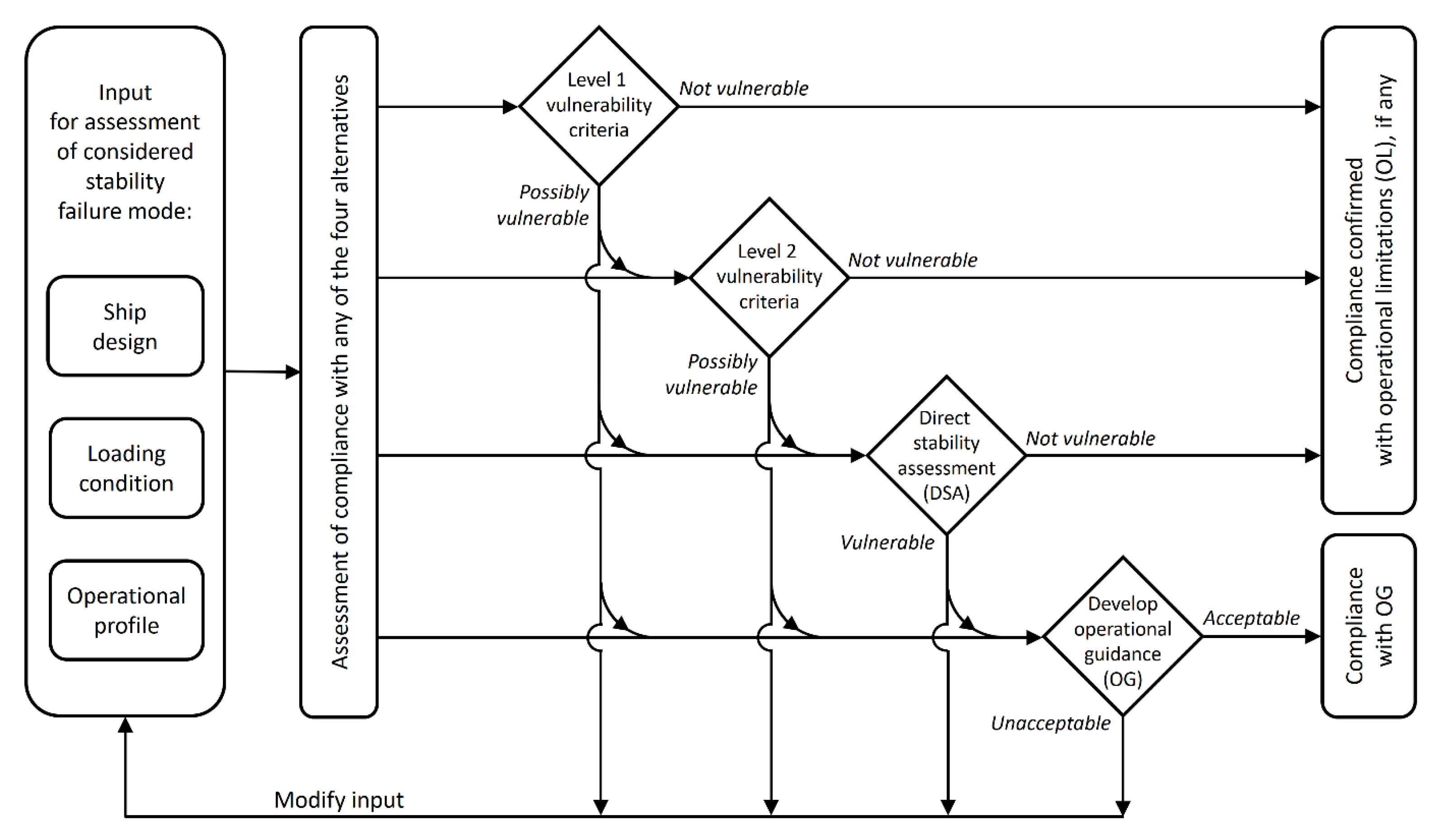
:1. Introduction
2. Methods
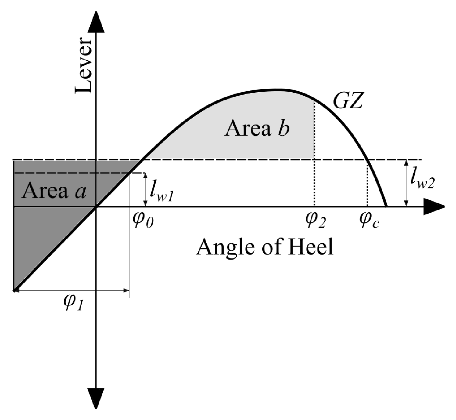
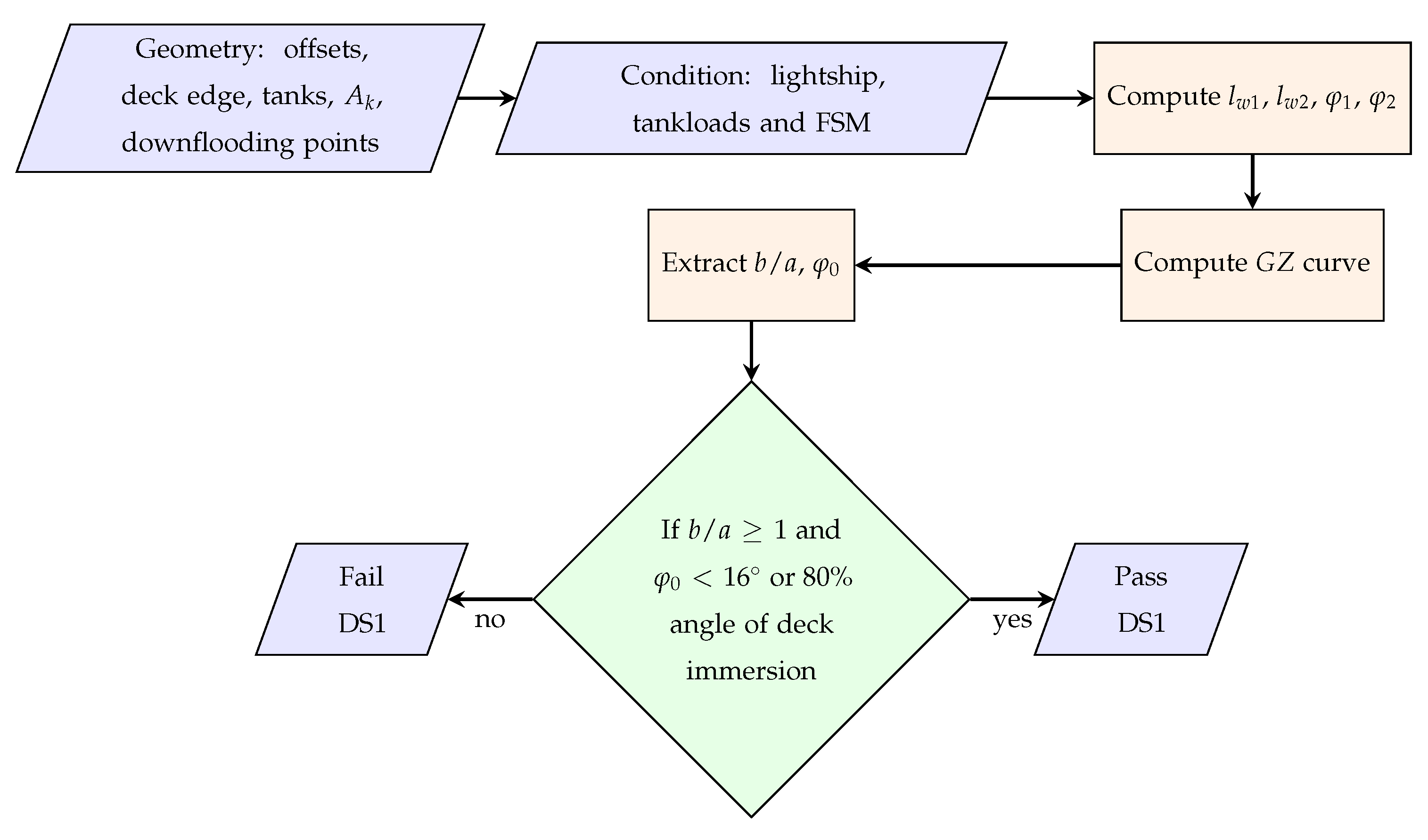
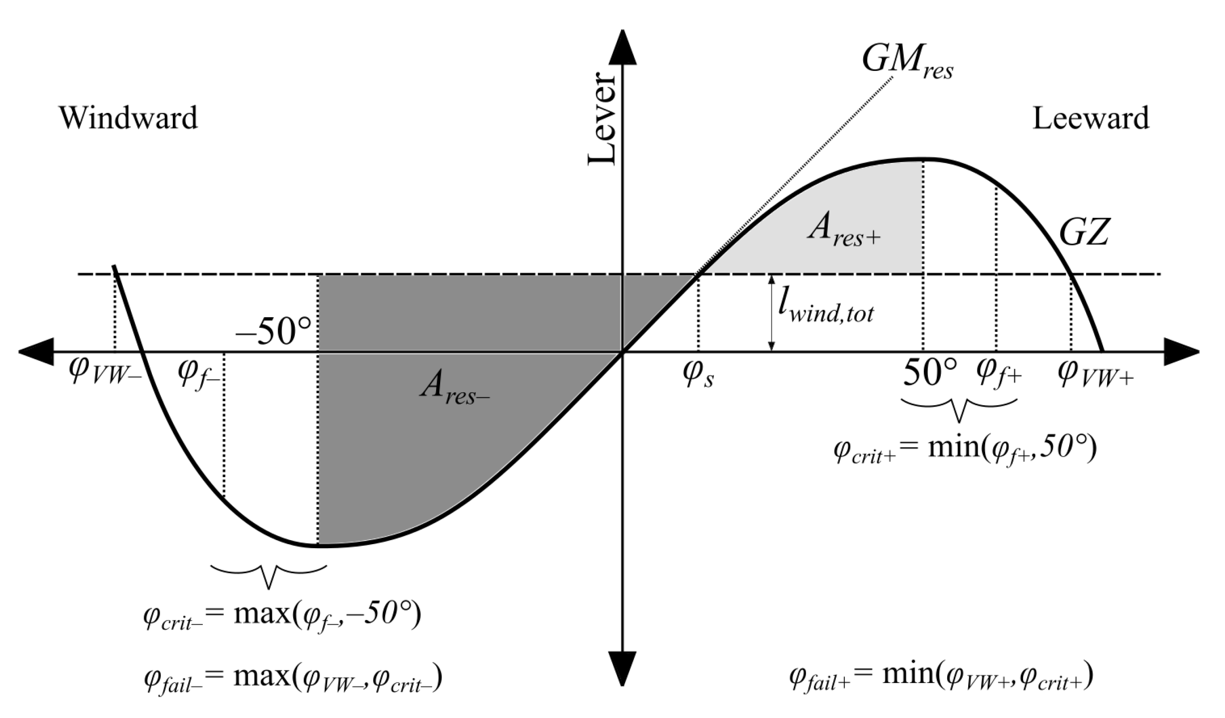
2.1. Dead Ship Condition (DS)
2.1.1. DS Level 1
2.1.2. DS Level 2
2.2. Excessive Acceleration (EA)
2.2.1. EA Level 1
2.2.2. EA Level 2
2.3. Pure Loss of Stability (PL)
2.3.1. PL Level 1
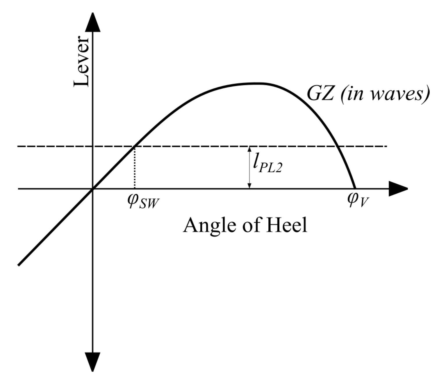
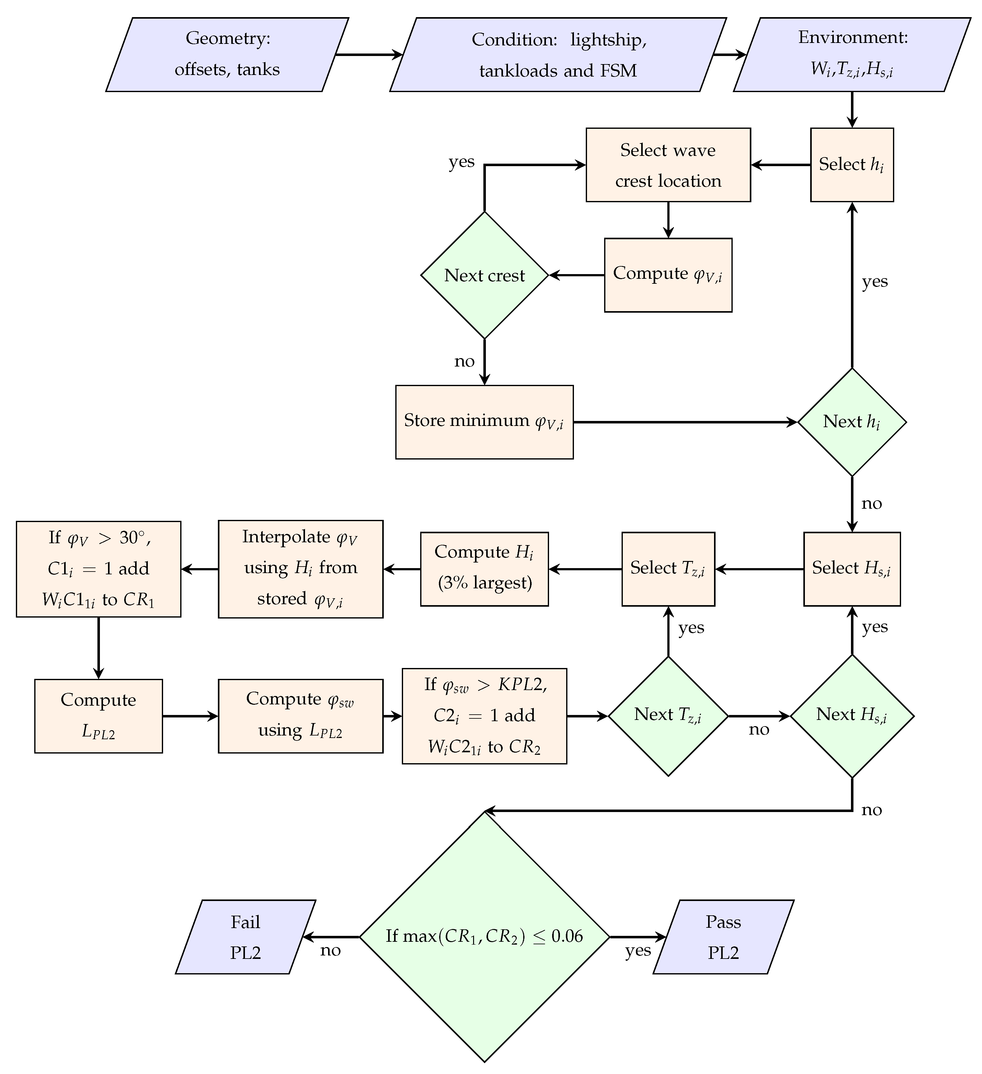
2.3.2. PL Level 2
2.4. Parametric Roll (PR)
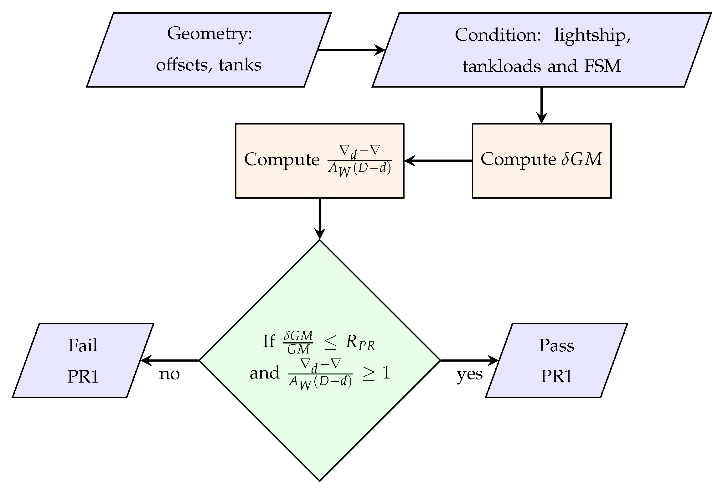
2.4.1. PR Level 1
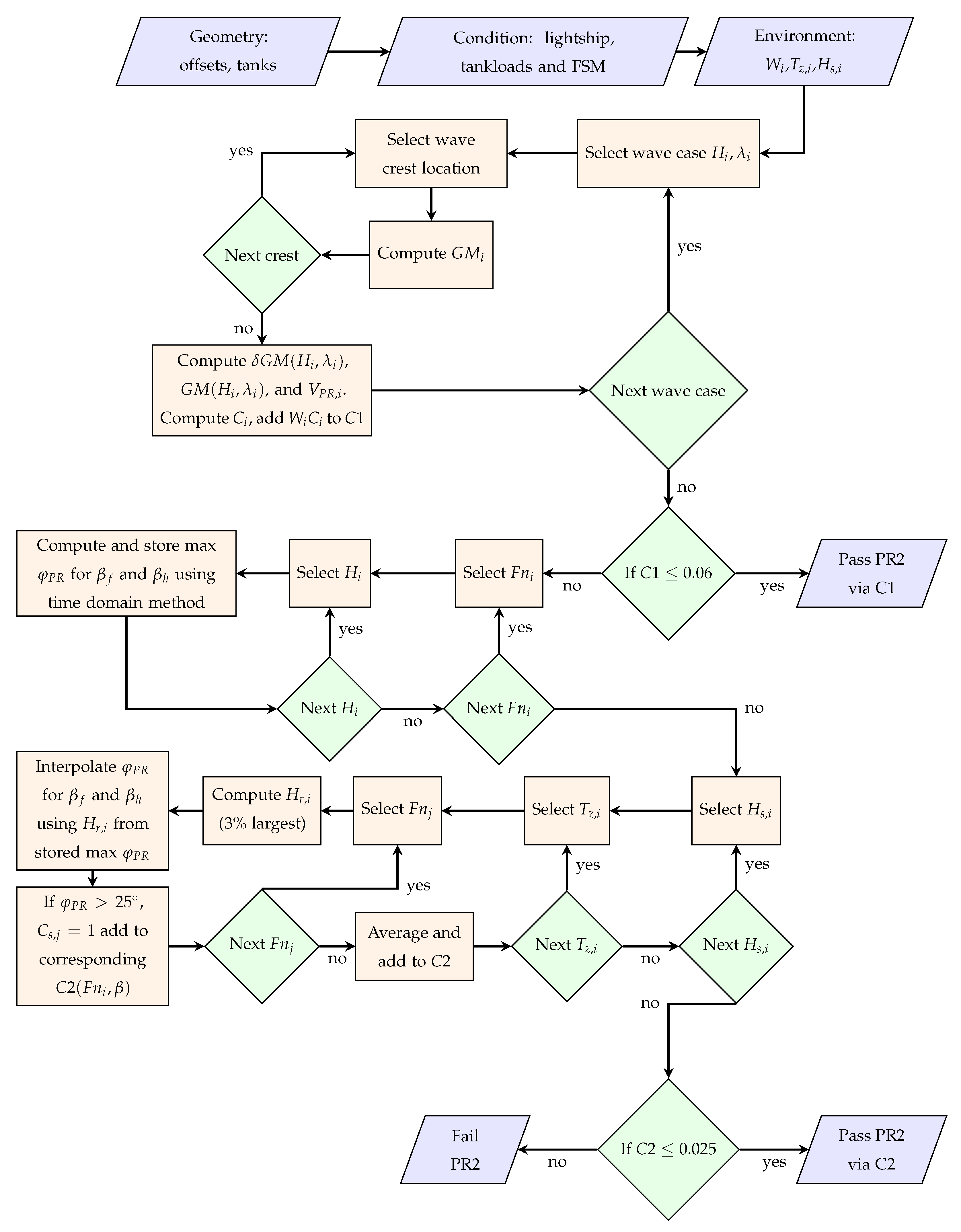
2.4.2. PR Level 2
2.5. Surf-Riding and Broaching (SB)
2.5.1. SB Level 1
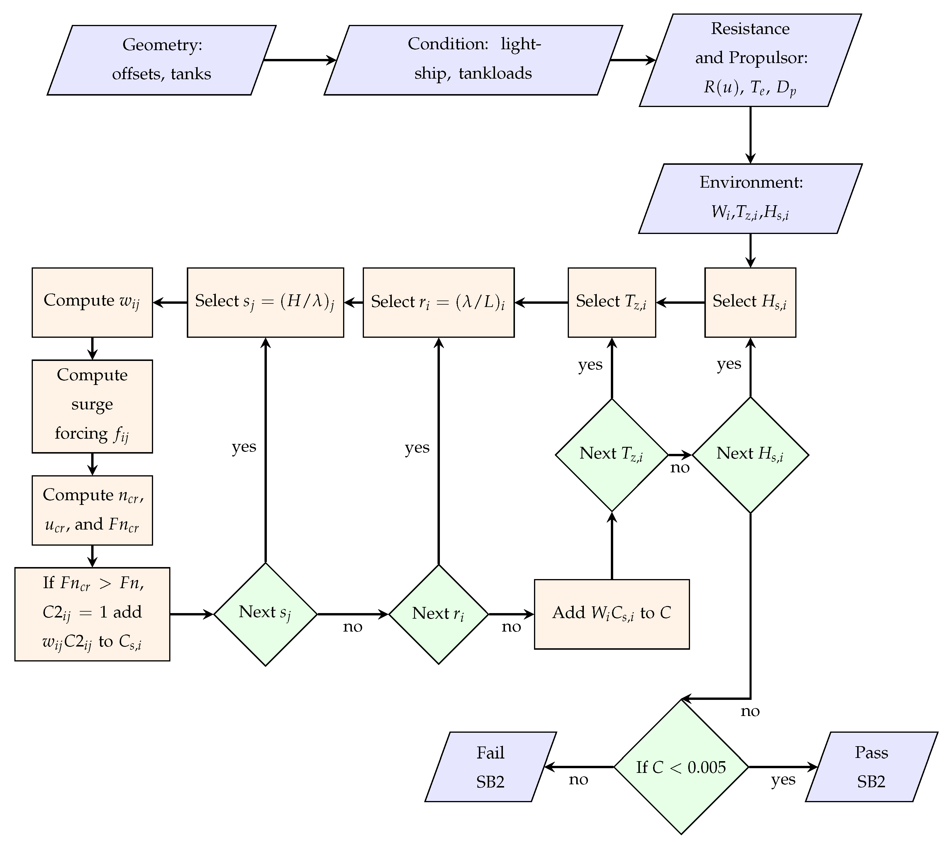
2.5.2. SB Level 2
3. Matrix Calculations
4. Environmental Input Parameters
5. Results
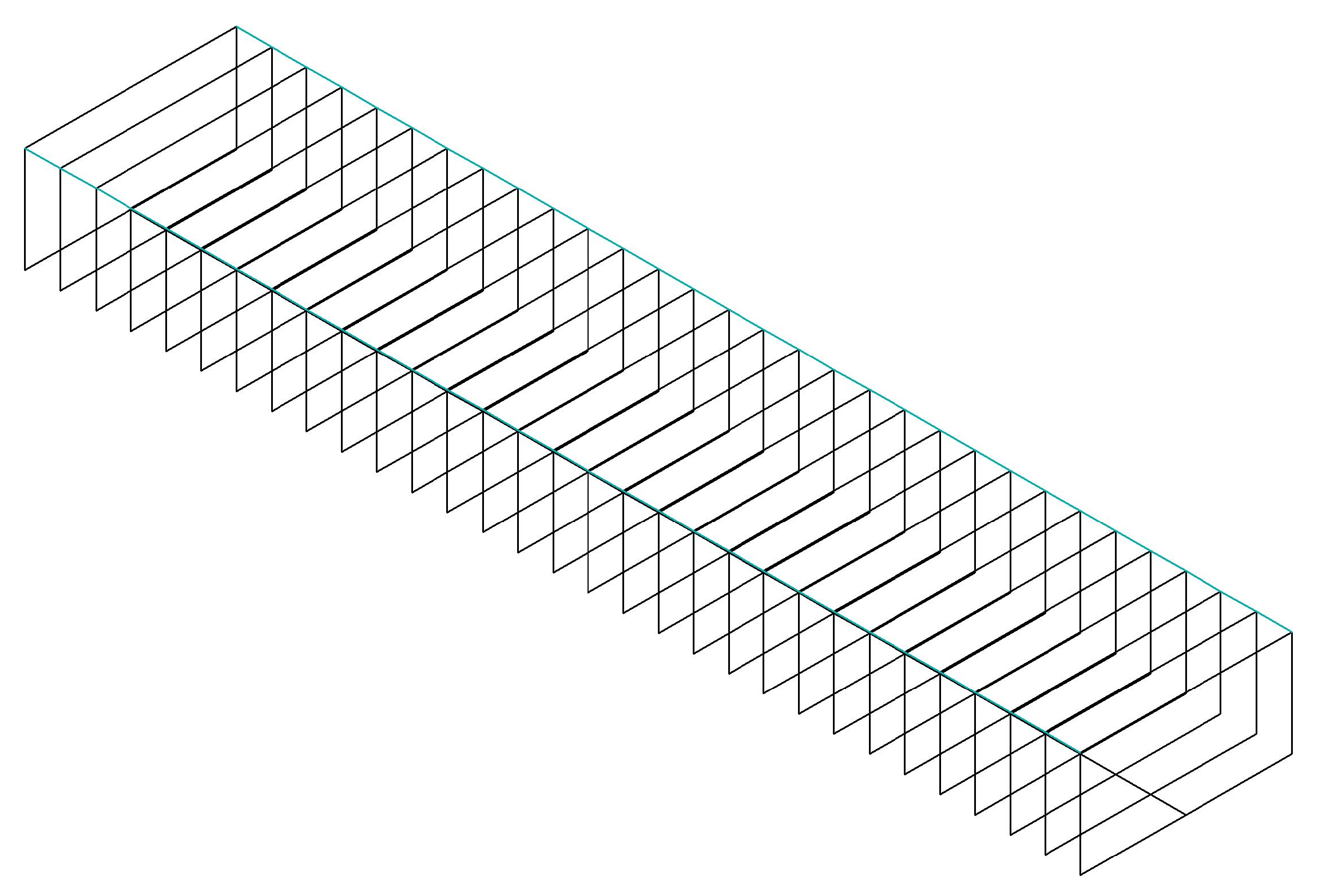
5.1. Barge
5.1.1. Level 1 Assessment of Dead Ship (DS) of Barge
5.1.2. Level 2 Assessment of Dead Ship (DS) for Barge
5.1.3. Level 1 Assessment of Excessive Acceleration (EA) for Barge
5.1.4. Level 2 Assessment of Excessive Acceleration (EA) for Barge
5.1.5. Level 1 Assessment of Pure Loss of Stability (PL) for Barge
5.1.6. Level 2 Assessment of Pure Loss of Stability (PL) for Barge
5.1.7. Level 1 Assessment of Parametric Roll (PR) for Barge
5.1.8. Level 2 Assessment of Parametric Roll (PR) for Barge
5.2. C11 Container Ship
5.2.1. Level 1 Assessment of Dead Ship (DS) for C11 Container Ship
5.2.2. Level 2 Assessment of Dead Ship (DS) for C11 Container Ship
5.2.3. Level 1 Assessment of Excessive Acceleration (EA) for C11 Container Ship
5.2.4. Level 2 Assessment of Excessive Acceleration (EA) for C11 Container Ship
5.2.5. Level 1 Assessment of Pure Loss of Stability (PL) for C11 Container Ship
5.2.6. Level 2 Assessment of Pure Loss of Stability (PL) for C11 Container Ship
5.2.7. Level 1 Assessment of Parametric Roll (PR) for C11 Container Ship
5.2.8. Level 2 Assessment of Parametric Roll (PR) for C11 Container Ship
5.3. KCS Container Ship
5.3.1. Level 1 Assessment of Dead Ship (DS) for KCS Container Ship
5.3.2. Level 2 Assessment of Dead Ship (DS) for KCS Container Ship
5.3.3. Level 1 Assessment of Excessive Acceleration (EA) for KCS Container Ship
5.3.4. Level 2 Assessment of Excessive Acceleration (EA) for KCS Container Ship
5.3.5. Level 1 Assessment of Pure Loss of Stability (PL) for KCS Container Ship
5.3.6. Level 2 Assessment of Pure Loss of Stability (PL) for KCS Container Ship
5.3.7. Level 1 Assessment of Parametric Roll (PR) for KCS Container Ship
5.3.8. Level 2 Assessment of Parametric Roll (PR) for KCS Container Ship
5.3.9. Level 1 Assessment of Surf-Riding and Broaching (SB) for KCS Container Ship
5.3.10. Level 2 Assessment of Surf-Riding and Broaching (SB) for KCS Container Ship
5.4. Fishing Vessel
5.4.1. Level 1 Assessment of Surf-Riding and Broaching (SB) for Fishing Vessel
5.4.2. Level 2 Assessment of Surf-Riding and Broaching (SB) for Fishing Vessel
6. Discussion
Author Contributions
Funding
Institutional Review Board Statement
Informed Consent Statement
Data Availability Statement
Acknowledgments
Conflicts of Interest
Abbreviations
| ABS | American Bureau of Shipping |
| CSI | Creative Systems, Inc. |
| GHS | General HydroStatics |
| IMO | International Maritime Organization |
| CRS | Cooperative Research Ship |
| RAO | Response Amplitude Operator |
| SGIS | Second Generation Intact Stability |
| DS | Dead Ship |
| EA | Excessive Acceleration |
| PL | Pure loss of stability |
| PR | Parametric Roll |
| SB | Surf-riding and Broaching |
References
- IMO. SDC 7/WP.6 Finalization of Second Generation Intact Stability Criteria—Report of the Drafting Group on Intact Stability; IMO: London, UK, 2020. [Google Scholar]
- IMO. MSC.1-Circ.1627 Interim Guidelines on the Second Generation Intact Stability Criteria; IMO: London, UK, 2020. [Google Scholar]
- Tompuri, M.; Ruponen, P.; Forss, M.; Lindroth, D. Application of the Second Generation Intact Stability Criteria in Initial Ship Design. In Proceedings of the SNAME Maritime Convention, Houston, TX, USA, 22–24 October 2014. [Google Scholar]
- Ariffin, A.; Mansor, S.; Laurnes, J.-M. A Numerical Study for Level 1 Second Generation Intact Stability Criteria. In Proceedings of the 12th International Conference on the Stability of Ships and Ocean Vehicles, Glasgow, UK, 14–19 June 2015.
- IMO. SDC 4-5-1/Add.1/2/3/4/5 Report of Correspondence Group (Parts 2–6); IMO: London, UK, 2016. [Google Scholar]
- Schroter, C.; Lutzen, M.; Erichsen, H.; Jensen, J.J.; Kristensen, H.O.; Hagelskjaer Lauridsen, P.; Tunccan, O.; Baltersen, J.P. Sample Applications of the Second Generation Intact Stability Criteria—Robustness and Consistency Analysis. In Proceedings of the 16th International Ship Stability Workshop, Belgrade, Serbia, 5–7 June 2017. [Google Scholar]
- Gonzalez, M.M.; Casas, V.D.; Rojas, L.P.; Agras, D.P.; Ocampo, F.J. Investigation of the Applicability of the IMO Second Generation Intact Stability Criteria to Fishing Vessels. In Proceedings of the 12th International Conference on the Stability of Ships and Ocean Vehicles, Glasgow, UK, 14–19 June 2015. [Google Scholar]
- Peters, W.; Belenky, V.; Bassler, C.; Spyrou, K.; Umeda, N.; Bulian, N.; Altmayer, B. The Second Generation Intact Stability Criteria: An Overview of Development. SNAME Trans. 2011, 121. [Google Scholar]
- Bulian, G.; Francescutto, A. A simplified modular approach for the prediction of the roll motion due to the combined action of wind and waves. Proc. Inst. Mech. Eng. Part M J. Eng. Marit. Environ. 2004, 218, 189–212. [Google Scholar] [CrossRef]
- Wandji, C.; Corrignan, P. Sample Application of Second Generation IMO Intact Stability Vulnerability Criteria as Updated during SLF 55. In Proceedings of the 13th International Ship Stability Workshop, Brest, France, 23–26 September 2013. [Google Scholar]
- Umeda, N.; Francescutto, A. Current state of the Second Generation Intact Stability criteria—Achievements and remaining issues. In Proceedings of the 15th International Ship Stability Workshop, Stockholm, Sweden, 13–15 June 2016. [Google Scholar]
- Shin, D.M.; Chung, J. Application of dead ship condition based on IMO second-generation intact stability criteria for 13K oil chemical tanker. Ocean. Eng. 2021, 238, 109776. [Google Scholar] [CrossRef]
- Petacco, N.; Pitardi, D.; Podenzana Bonvino, C.; Gualeni, P. Application of the IMO Second Generation Intact Stability Criteria to a Ballast-Free Container Ship. J. Mar. Sci. Eng. 2021, 9, 1416. [Google Scholar] [CrossRef]
- Boccadamo, G.; Rosano, G. Excessive Acceleration Criterion: Application to Naval Ships. J. Mar. Sci. Eng. 2019, 7, 431. [Google Scholar] [CrossRef] [Green Version]
- Shin, D.M.; Moon, B.Y.; Chung, J. Application of surf-riding and broaching mode based on IMO second-generation intact stability criteria for previous ships. Int. J. Nav. Archit. Ocean. Eng. 2021, 13, 545–553. [Google Scholar] [CrossRef]
- Umeda, N.; Usada, S.; Mizumoto, K.; Matsuda, A. Broaching probability for a ship in irregular stern-quartering waves: Theoretical prediction and experimental validation. J. Mar. Sci. Technol. 2016, 21, 23–37. [Google Scholar] [CrossRef] [Green Version]
- Gualeni, P.; Paolodello, D.; Petacco, N.; Lena, C. Seakeeping time domain simulations for surf-riding/broaching: Investigations toward a direct stability assessment. J. Mar. Sci. Technol. 2020, 25, 1120–1128. [Google Scholar] [CrossRef]
- Bu, S.X.; Gu, M.; Abdel-Maksoud, M. Study on Roll Restoring Arm Variation Using a Three-Dimensional Hybrid Panel Method. J. Ship Res. 2019, 63, 94–107. [Google Scholar] [CrossRef]
- Lu, J.; Gu, M.; Boulougouris, E. Model experiments and direct stability assessments on pure loss of stability of the ONR tumblehome in following seas. Ocean. Eng. 2019, 194, 106640. [Google Scholar] [CrossRef]
- Gu, M.; Bu, S.; Lu, J. Study of parametric roll in oblique waves using a three-dimensional hybrid panel method. J. Hydrodyn. 2020, 32, 126–138. [Google Scholar] [CrossRef]
- Lu, J.; Gu, M.; Boulougouris, E. Model experiments and direct stability assessments on pure loss of stability in stern quartering waves. Ocean. Eng. 2020, 216, 108035. [Google Scholar] [CrossRef]
- Bulian, G.; Francescutto, A. Second Generation Intact Stability Criteria: On the validation of codes for direct stability assessment in the framework of an example application. Pol. Marit. Res. 2013, 4, 52–61. [Google Scholar] [CrossRef] [Green Version]
- Lu, J.; Gu, M.; Umeda, N. Experimental and numerical study on several crucial elements for predicting parametric roll in regular head seas. J. Mar. Sci. Technol. 2017, 22, 25–37. [Google Scholar] [CrossRef]
- Kapsenberg, G.; Wandji, C.; Duz, B.; Kim, P.S. A Comparison of Numerical Simulations and Model Experiments on Parametric Roll in Irregular Seas. J. Mar. Sci. Eng. 2020, 8, 474. [Google Scholar] [CrossRef]
- IACS. No. 34 Standard Wave Data; IACS: London, UK, 2001. [Google Scholar]
- IMO. International Code of Intact Stability; IMO: London, UK, 2008. [Google Scholar]
- Rudakovic, S.; Bulian, G.; Backalov, I. Effective wave slope coefficient of river-sea ships. Ocean. Eng. 2019, 192, 106427. [Google Scholar] [CrossRef]
- ITTC. Numerical Estimation of Roll Damping; ITTC: Zurich, Switzerland, 2011. [Google Scholar]
- Wilson, R.V.; Carrica, P.M.; Stern, F. Unsteady URANS method for ship motions with application to roll for a surface combatant. Comput. Fluids 2006, 35, 501–524. [Google Scholar] [CrossRef]
- Kianejad, S.S.; Enshaei, H.; Duffy, J.; Ansarifard, N.; Ranmuthugala, D. Ship Roll Damping Coefficient Prediction Using CFD. J. Ship Res. 2019, 63, 108–122. [Google Scholar] [CrossRef]
- Alexandersson, M.; Mao, W.; Ringsberg, J.W. Analysis of roll damping model scale data. Ships Offshore Struct. 2021, 16, 85–92. [Google Scholar] [CrossRef]
- Ikeda, Y.; Himeno, Y.; Tanaka, N. On Eddy Making Component of Roll Damping Force on Naked Hull; University of Osaka Prefecture, Department of Naval Architecture: Osaka, Japan, 1978. [Google Scholar]
- Ikeda, Y.; Himeno, Y.; Tanaka, N. Components of Roll Damping of Ship at Forward Speed; University of Osaka Prefecture, Department of Naval Architecture: Osaka, Japan, 1978. [Google Scholar]
- Ikeda, Y.; Komatsu, K.; Himeno, Y.; Tanaka, N. On Roll Damping Force of Ship—Effect of Hull Surface Pressure Created by Bilge Keels; University of Osaka Prefecture, Department of Naval Architecture: Osaka, Japan, 1978. [Google Scholar]
- Himeno, Y. Prediction of Ship Roll Damping–State of the Art; University of Michigan, Department of NA&ME: Ann Arbor, MI, USA, 1981. [Google Scholar]
- Ikeda, Y. On the Form of Nonlinear Roll Damping of Ships; Technical University of Berlin: Berlin, Germany, 1983. [Google Scholar]
- McTaggart, K. Appendage and Viscous Forces for Ship Motions in Waves; Defence Research and Development Canada—Atlantic Research Center: Dartmouth, Nova Scotia, 2004. [Google Scholar]
- Spanos, D.; Papanikolaou, A. SAFEDOR International Benchmark Study on Numerical Simulation Methods for the Prediction of Parametric Roll of Ships in Waves. In Proceedings of the 10th International Conference on Stability of Ships and Ocean Vehicles, St. Petersburg, Russia, 22–26 June 2009. [Google Scholar]
- Petacco, N.; Gualeni, P. IMO Second Generation Intact Stability Criteria: General Overview and Focus on Operational Measures. J. Mar. Sci. Eng. 2020, 8, 494. [Google Scholar] [CrossRef]
- Creative Systems, Inc. GHS-SK User Manual; Creative Systems, Inc.: Port Townsend, WA, USA, 2021. [Google Scholar]
- Cooperative Research Ships. CRS DYNASTY Technical Report Task 1.1 Documentation for IMO Levels 1&2 Tools; Bureau Veritas: Paris, France, 2018. [Google Scholar]


| (m) / (s) | 3.5 | 4.5 | 5.5 | 6.5 | 7.5 | 8.5 | 9.5 | 10.5 | 11.5 | 12.5 | 13.5 | 14.5 | 15.5 | 16.5 | 17.5 | 18.5 |
|---|---|---|---|---|---|---|---|---|---|---|---|---|---|---|---|---|
| 0.5 | 1.3 | 133.7 | 865.6 | 1186.0 | 634.2 | 186.3 | 36.9 | 5.6 | 0.7 | 0.1 | 0.0 | 0.0 | 0.0 | 0.0 | 0.0 | 0.0 |
| 1.5 | 0.0 | 29.3 | 986.0 | 4976.0 | 7738.0 | 5569.7 | 2375.7 | 703.5 | 160.7 | 30.5 | 5.1 | 0.8 | 0.1 | 0.0 | 0.0 | 0.0 |
| 2.5 | 0.0 | 2.2 | 197.5 | 2158.8 | 6230.0 | 7449.5 | 4960.4 | 2066.0 | 644.5 | 160.2 | 33.7 | 6.3 | 1.1 | 0.2 | 0.0 | 0.0 |
| 3.5 | 0.0 | 0.2 | 34.9 | 695.5 | 3226.5 | 5675.0 | 5099.1 | 2838.0 | 1114.1 | 337.7 | 84.3 | 18.2 | 3.5 | 0.6 | 0.1 | 0.0 |
| 4.5 | 0.0 | 0.0 | 6.0 | 196.1 | 1354.3 | 3288.5 | 3857.5 | 2685.5 | 1275.2 | 455.1 | 130.9 | 31.9 | 6.9 | 1.3 | 0.2 | 0.0 |
| 5.5 | 0.0 | 0.0 | 1.0 | 51.0 | 498.4 | 1602.9 | 2372.7 | 2008.3 | 1126.0 | 463.6 | 150.9 | 41.0 | 9.7 | 2.1 | 0.4 | 0.1 |
| 6.5 | 0.0 | 0.0 | 0.2 | 12.6 | 167.0 | 690.3 | 1257.9 | 1268.6 | 825.9 | 386.8 | 140.8 | 42.2 | 10.9 | 2.5 | 0.5 | 0.1 |
| 7.5 | 0.0 | 0.0 | 0.0 | 3.0 | 52.1 | 270.1 | 594.4 | 703.2 | 524.9 | 276.7 | 111.7 | 36.7 | 10.2 | 2.5 | 0.6 | 0.1 |
| 8.5 | 0.0 | 0.0 | 0.0 | 0.7 | 15.4 | 97.9 | 255.9 | 350.6 | 296.9 | 174.6 | 77.6 | 27.7 | 8.4 | 2.2 | 0.5 | 0.1 |
| 9.5 | 0.0 | 0.0 | 0.0 | 0.2 | 4.3 | 33.2 | 101.9 | 159.9 | 152.2 | 99.2 | 48.3 | 18.7 | 6.1 | 1.7 | 0.4 | 0.1 |
| 10.5 | 0.0 | 0.0 | 0.0 | 0.0 | 1.2 | 10.7 | 37.9 | 67.5 | 71.7 | 51.5 | 27.3 | 11.4 | 4.0 | 1.2 | 0.3 | 0.1 |
| 11.5 | 0.0 | 0.0 | 0.0 | 0.0 | 0.3 | 3.3 | 13.3 | 26.6 | 31.4 | 24.7 | 14.2 | 6.4 | 2.4 | 0.7 | 0.2 | 0.1 |
| 12.5 | 0.0 | 0.0 | 0.0 | 0.0 | 0.1 | 1.0 | 4.4 | 9.9 | 12.8 | 11.0 | 6.8 | 3.3 | 1.3 | 0.4 | 0.1 | 0.0 |
| 13.5 | 0.0 | 0.0 | 0.0 | 0.0 | 0.0 | 0.3 | 1.4 | 3.5 | 5.0 | 4.6 | 3.1 | 1.6 | 0.7 | 0.2 | 0.1 | 0.0 |
| 14.5 | 0.0 | 0.0 | 0.0 | 0.0 | 0.0 | 0.1 | 0.4 | 1.2 | 1.8 | 1.8 | 1.3 | 0.7 | 0.3 | 0.1 | 0.0 | 0.0 |
| 15.5 | 0.0 | 0.0 | 0.0 | 0.0 | 0.0 | 0.0 | 0.1 | 0.4 | 0.6 | 0.7 | 0.5 | 0.3 | 0.1 | 0.1 | 0.0 | 0.0 |
| 16.5 | 0.0 | 0.0 | 0.0 | 0.0 | 0.0 | 0.0 | 0.0 | 0.1 | 0.2 | 0.2 | 0.2 | 0.1 | 0.1 | 0.1 | 0.0 | 0.0 |
| Parameter | Description | Applicable Failure Modes |
|---|---|---|
| P | Wind pressure | DS |
| Wind speed | DS | |
| Gustiness spectrum | DS | |
| s | Wave steepness factor | DS, EA, SB |
| Short-term seaway probability of occurrence | DS, EA, PL, PR, SB | |
| Short-term seaway significant wave height | DS, EA, PL, PR, SB | |
| Short-term seaway peak period | DS, EA, PL, PR, SB | |
| Short-term wave spectrum | DS, EA, PL, PR | |
| r | Wavelength to ship length ratio | SB |
| Ship speed | PR, SB |
| L | 100.00 | m |
| B | 20.00 | m |
| D | 10.00 | m |
| 5.00 | m | |
| 1.00 | ||
| 1.00 | ||
| 5.00 | knots | |
| 50.00 | m |
| 5 | m | Daft at aft perpendicular | |
| 5 | m | Draft at forward perpendicular | |
| 7 | m | Vertical center of gravity | |
| 2.167 | m | Metacentric height | |
| ∇ | 10,000 | m | Volumetric displacement |
| 12 | s | Natural roll period | |
| 500 | m | Projected lateral area above WL | |
| Z | 5 | m | Vertical distance from to center of |
| 40 | deg | Angle at which openings immerse | |
| z | 40 | m | Highest vertical location of the crew area from BL |
| x | 30 | m | Longitudinal distance of the location of the crew from AP |
| Level 1 Dead Ship Condition | ABS | CSI |
|---|---|---|
| Area A | 3.083 | 2.947 |
| Area B | 33.652 | 35.079 |
| Ratio of B/A | 10.917 | 11.904 |
| Check if B/A > 1 | Pass | Pass |
| Level 2 Dead Ship Condition | ABS | CSI |
|---|---|---|
| C | 0.000 | |
| 0.06 | 0.06 | |
| Check if | Pass | Pass |
| Level 1 Excessive Acceleration | ABS | CSI |
|---|---|---|
| r effective wave slope | 0.910 | 0.910 |
| s wave steepness | 0.032 | 0.032 |
| characteristic roll amplitude (rad) | 0.093 | 0.091 |
| acceleration estimated (m/s) | 1.221 | 1.2 |
| (m/s) | 4.64 | 4.64 |
| Check if | Pass | Pass |
| Level 2 Excessive Acceleration | ABS | CSI |
|---|---|---|
| C | 0.000 | 0 |
| 0.00039 | 0.00039 | |
| Check if | Pass | Pass |
| Level 1 Pure Loss of Stability | ABS | CSI |
|---|---|---|
| Displacement Ratio | 1.00 | 1.00 |
| Check if Displacement Ratio ≥ 1 | Pass | Pass |
| 3.33 | 3.397 | |
| 66,667 | 66,667 | |
| 2.5 | 2.5 | |
| 2.167 | 2.167 | |
| 0.05 | 0.05 | |
| Check if | Pass | Pass |
| Level 2 Pure Loss of Stability | ABS | CSI |
|---|---|---|
| 0 | 0 | |
| 0.03 | 0 | |
| 0.06 | 0.06 | |
| Check if | Pass | Pass |
| Level 1 Parametric Roll | ABS | CSI |
|---|---|---|
| Displacement Ratio | 1.00 | 1.00 |
| Check if Displacement Ratio ≥ 1 | Pass | Pass |
| 0.0 | ||
| 2.167 | ||
| 0.000 | 0.000 | |
| 1.23 | 1.28 | |
| Check if | Pass | Pass |
| Level 1 Parametric Roll | ABS | CSI |
|---|---|---|
| 0 | 0 | |
| 0.06 | 0.06 | |
| 0.000 | N/A | |
| 0.025 | N/A | |
| Check if | Pass | Pass |
| L | 262.00 | m |
| B | 40.00 | m |
| D | 24.45 | m |
| 12.5 | m | |
| 0.56 | - | |
| 0.96 | - | |
| 24.5 | knots | |
| 61.02 | m |
| 11.50 | m | Daft at aft perpendicular | |
| 11.50 | m | Draft at forward perpendicular | |
| 18.40 | m | Vertical center of gravity | |
| 1.40 | m | Metacentric height | |
| ∇ | 67,384.00 | m | Volumetric displacement |
| 25.10 | s | Natural roll period | |
| 7093.00 | m | Projected lateral area above WL | |
| Z | 7.71 | m | Vertical distance from to center of |
| 50.00 | deg | Angle at which openings immerse | |
| z | 40.00 | m | Highest vertical location of crew area from BL |
| x | 30.00 | m | Longitudinal distance of the location of the crew from AP |
| Level 1 Dead Ship Condition | ABS | CSI |
|---|---|---|
| Area A | 3.481 | 4.675 |
| Area B | 36.275 | 41.075 |
| Ratio of B/A | 10.420 | 8.774 |
| Check if B/A > 1 | Pass | Pass |
| Level 2 Dead Ship Condition | ABS | CSI | CRS |
|---|---|---|---|
| C | 0.000 | ||
| 0.06 | 0.06 | 0.06 | |
| Check if | Pass | Pass | Pass |
| Level 1 Excessive Acceleration | ABS | CSI |
|---|---|---|
| r effective wave slope | 0.942 | 0.940 |
| s wave steepness | 0.024 | 0.024 |
| characteristic roll amplitude (rad) | 0.133 | 0.123 |
| acceleration estimated (m/s) | 1.600 | 1.476 |
| (m/s) | 4.64 | 4.64 |
| Check if | Pass | Pass |
| Level 2 Excessive Acceleration | ABS | CSI |
|---|---|---|
| C | 0.000 | 0 |
| 0.00039 | 0.00039 | |
| Check if | Pass | Pass |
| Level 1 Pure Loss of Stability | ABS | CSI | CRS |
|---|---|---|---|
| Displacement Ratio | 1.191 | 1.2 | |
| Check if Displacement Ratio ≥ 1 | Pass | Pass | Pass |
| 7.1246 | 7.118 | ||
| 659,945 | 657,754 | ||
| 6.537 | 6.54 | ||
| −2.069 | −2.1 | −2.065 | |
| 0.05 | 0.05 | 0.05 | |
| Check if | Fail | Fail | Fail |
| Level 2 Pure Loss of Stability | ABS | CSI |
|---|---|---|
| 0 | 0 | |
| 0.004 | 0.01 | |
| 0.06 | 0.06 | |
| Check if | Pass | Pass |
| Level 1 Parametric Roll | ABS | CSI | CRS |
|---|---|---|---|
| Displacement Ratio | 1.191 | 1.2 | |
| Check if Displacement Ratio ≥ 1 | Pass | Pass | Pass |
| 2.187 | 2.5491 | ||
| 1.990 | 1.944 | ||
| 1.099 | 1.310 | 1.097 | |
| 0.420 | 0.420 | 0.420 | |
| Check if | Fail | Fail | Fail |
| Level 1 Parametric Roll | ABS | CSI | CRS |
|---|---|---|---|
| 0.436 | 0.440 | 0.436 | |
| 0.06 | 0.06 | 0.06 | |
| 0.074 | 0.090 | 0.1 | |
| 0.025 | 0.025 | 0.025 | |
| Check if | Fail | Fail | Fail |
| L | 230.00 | m |
| B | 32.20 | m |
| D | 17.20 | m |
| 11.0 | m | |
| 0.64 | - | |
| 0.94 | - | |
| 24.0 | knots | |
| 64.00 | m |
| 10.80 | m | Daft at aft perpendicular | |
| 10.80 | m | Draft at forward perpendicular | |
| 13.674 | m | Vertical center of gravity | |
| 1.32 | m | Metacentric height | |
| ∇ | 54,148.00 | m | Volumetric displacement |
| 25.10 | s | Natural roll period | |
| 6000.00 | m | Projected lateral area above WL | |
| Z | 12.00 | m | Vertical distance from to center of |
| 50.00 | deg | Angle at which openings immerse | |
| z | 35.00 | m | Highest vertical location of crew area from BL |
| x | 30.00 | m | Longitudinal distance of the location of the crew from AP |
| 7.9 | m | Propeller diameter | |
| 0.13 | - | Thrust fraction | |
| 0.26 | - | Wake fraction | |
| 0 | N | 0th-order resistance regression coefficient | |
| 375,181.0 | N/(m/s) | 1st-order resistance regression coefficient | |
| −255,614.0 | N/(m/s) | 2nd-order resistance regression coefficient | |
| 63,275.0 | N/(m/s) | 3rd-order resistance regression coefficient | |
| −6149.0 | N/(m/s) | 4th-order resistance regression coefficient | |
| 210.34 | N/(m/s) | 5th-order resistance regression coefficient | |
| 0.53 | - | 0th-order thrust regression coefficient | |
| −0.48 | - | 1st-order thrust regression coefficient | |
| −0.02 | - | 2nd-order thrust regression coefficient |
| Level 1 Dead Ship Condition | ABS | CSI |
|---|---|---|
| Area A | 2.780 | 2.896 |
| Area B | 13.684 | 12.167 |
| Ratio of B/A | 4.922 | 4.135 |
| Check if B/A > 1 | Pass | Pass |
| Level 2 Dead Ship Condition | ABS | CSI |
|---|---|---|
| C | 0.000 | |
| 0.06 | 0.06 | |
| Check if | Pass | Pass |
| Level 1 Excessive Acceleration | ABS | CSI |
|---|---|---|
| r effective wave slope | 0.932 | 0.939 |
| s wave steepness | 0.024 | 0.024 |
| characteristic roll amplitude (rad) | 0.132 | 0.133 |
| acceleration estimated (m/s) | 1.552 | 1.53 |
| (m/s) | 4.64 | 4.64 |
| Check if | Pass | Pass |
| Level 2 Excessive Acceleration | ABS | CSI |
|---|---|---|
| C | 0.000 | 0 |
| 0.00039 | 0.00039 | |
| Check if | Pass | Pass |
| Level 1 Pure Loss of Stability | ABS | CSI |
|---|---|---|
| Displacement Ratio | 1.004 | 1.09 |
| Check if Displacement Ratio ≥ 1 | Pass | Pass |
| 6.974 | ||
| 360,118 | ||
| 5.94 | ||
| −1.062 | −0.76 | |
| 0.05 | 0.05 | |
| Check if | Fail | Fail |
| Level 2 Pure Loss of Stability | ABS | CSI |
|---|---|---|
| 0.045 | 0.04 | |
| 0 | 0 | |
| 0.06 | 0.06 | |
| Check if | Pass | Pass |
| Level 1 Parametric Roll | ABS | CSI |
|---|---|---|
| Displacement Ratio | 1.004 | 1.09 |
| Check if Displacement Ratio ≥ 1 | Pass | Pass |
| 0.991 | 1.2271 | |
| 1.327 | 1.303 | |
| 0.747 | 0.94 | |
| 0.354 | 0.35 | |
| Check if | Fail | Fail |
| Level 2 Parametric Roll | ABS | CSI |
|---|---|---|
| 0.436 | 0.436 | |
| 0.06 | 0.06 | |
| 0.062 | 0.12 | |
| 0.025 | 0.025 | |
| Check if | Fail | Fail |
| Level 1 Surf-Riding and Broaching | ABS | CSI |
|---|---|---|
| Check if 200 m | Pass | Pass |
| 0.26 | 0.26 | |
| Check if | Pass | Pass |
| Level 2 Surf-Riding and Broaching | ABS | CSI |
|---|---|---|
| C | 0.000 | 0.001 |
| 0.005 | 0.005 | |
| Check if | Pass | Pass |
| L | 34.5 | m |
| B | 7.6 | m |
| D | 3.5 | m |
| 2.65 | m | |
| 0.60 | - | |
| 0.97 | - | |
| 14.29 | knots |
| 2.65 | m | Draft at aft perpendicular | |
| 2.65 | m | Draft at forward perpendicular | |
| 0 | m | Vertical center of gravity | |
| 2.988 | m | Metacentric height | |
| ∇ | 414.81 | m | Volumetric displacement |
| 25.1 | s | Natural roll period | |
| 7093 | m | Projected lateral area above WL | |
| Z | 8.208 | m | Vertical distance from to center of |
| 40.15 | deg | Angle at which openings immerse | |
| z | 10 | m | Highest vertical location of crew area from BL |
| x | 10 | m | Longitudinal distance of the location of the crew from AP |
| 2.6 | m | Propeller diameter | |
| 0.142 | - | Thrust fraction | |
| 0.156 | - | Wake fraction | |
| 0 | N | 0th-order resistance regression coefficient | |
| −435.63 | N/(m/s) | 1st-order resistance regression coefficient | |
| 763.62 | N/(m/s) | 2nd-order resistance regression coefficient | |
| −271.98 | N/(m/s) | 3rd-order resistance regression coefficient | |
| 41.611 | N/(m/s) | 4th-order resistance regression coefficient | |
| −1.7335 | N/(m/s) | 5th-order resistance regression coefficient | |
| 0.2244 | - | 0th-order thrust regression coefficient | |
| −0.2283 | - | 1st-order thrust regression coefficient | |
| −0.1373 | - | 2nd-order thrust regression coefficient |
| Level 1 Surf-Riding and Broaching | ABS | CSI | IMO |
|---|---|---|---|
| Check if 200 m | Fail | Fail | Fail |
| 0.4 | 0.4 | 0.4 | |
| Check if | Fail | Fail | Fail |
| Level 2 Surf-Riding and Broaching | ABS | CSI | IMO |
|---|---|---|---|
| C | 0.0586 | 0.07 | 0.0591 |
| 0.005 | 0.005 | 0.005 | |
| Check if | Fail | Fail | Fail |
| Ship | Failure Mode | Level | ABS | CSI | CRS | IMO |
|---|---|---|---|---|---|---|
| Barge | Dead Ship | 1 | Pass | Pass | ||
| 2 | Pass | Pass | ||||
| Excessive Acceleration | 1 | Pass | Pass | |||
| 2 | Pass | Pass | ||||
| Pure Loss of Stability | 1 | Pass | Pass | |||
| 2 | Pass | Pass | ||||
| Parametric Rolling | 1 | Pass | Pass | |||
| 2 | Pass | Pass | ||||
| C11 Container Ship | Dead Ship | 1 | Pass | Pass | ||
| 2 | Pass | Pass | Pass | |||
| Excessive Acceleration | 1 | Pass | Pass | |||
| 2 | Pass | Pass | ||||
| Pure Loss of Stability | 1 | Fail | Fail | Fail | ||
| 2 | Pass | Pass | Pass | |||
| Parametric Rolling | 1 | Fail | Fail | Fail | ||
| 2 | Fail | Fail | Fail | |||
| KCS Container Ship | Dead Ship | 1 | Pass | Pass | ||
| 2 | Pass | Pass | ||||
| Excessive Acceleration | 1 | Pass | Pass | |||
| 2 | Pass | Pass | ||||
| Pure Loss of Stability | 1 | Fail | Fail | |||
| 2 | Pass | Pass | ||||
| Parametric Rolling | 1 | Fail | Fail | |||
| 2 | Fail | Fail | ||||
| Surf-riding and Broaching | 1 | Pass | Pass | |||
| 2 | Pass | Pass | ||||
| Fishing Vessel | Surf-riding and Broaching | 1 | Fail | Fail | Fail | |
| 2 | Fail | Fail | Fail |
Publisher’s Note: MDPI stays neutral with regard to jurisdictional claims in published maps and institutional affiliations. |
© 2021 by the authors. Licensee MDPI, Basel, Switzerland. This article is an open access article distributed under the terms and conditions of the Creative Commons Attribution (CC BY) license (https://creativecommons.org/licenses/by/4.0/).
Share and Cite
Marlantes, K.E.; Kim, S.; Hurt, L.A. Implementation of the IMO Second Generation Intact Stability Guidelines. J. Mar. Sci. Eng. 2022, 10, 41. https://doi.org/10.3390/jmse10010041
Marlantes KE, Kim S, Hurt LA. Implementation of the IMO Second Generation Intact Stability Guidelines. Journal of Marine Science and Engineering. 2022; 10(1):41. https://doi.org/10.3390/jmse10010041
Chicago/Turabian StyleMarlantes, Kyle E., Sungeun (Peter) Kim, and Lucas A. Hurt. 2022. "Implementation of the IMO Second Generation Intact Stability Guidelines" Journal of Marine Science and Engineering 10, no. 1: 41. https://doi.org/10.3390/jmse10010041
APA StyleMarlantes, K. E., Kim, S., & Hurt, L. A. (2022). Implementation of the IMO Second Generation Intact Stability Guidelines. Journal of Marine Science and Engineering, 10(1), 41. https://doi.org/10.3390/jmse10010041