Modelling of Parametric Resonance for Heaving Buoys with Position-Varying Waterplane Area

Abstract

Exploiting parametric resonance may enable increased performance for wave energy converters (WECs). By designing the geometry of a heaving WEC, it is possible to introduce a heave-to-heave Mathieu instability that can trigger parametric resonance. To evaluate the potential of such a WEC, a mathematical model is introduced in this paper for a heaving buoy with a non-constant waterplane area in monochromatic waves. The efficacy of the model in capturing parametric resonance is verified by a comparison against the results from a nonlinear Froude–Krylov force model, which numerically calculates the forces on the buoy based on the evolving wetted surface area. The introduced model is more than 1000 times faster than the nonlinear Froude–Krylov force model and also provides the significant benefit of enabling analytical investigation techniques to be utilised.

1. Introduction

Renewable energy sources are an attractive form of energy supply for the growing human population, since these resources are inexhaustible and clean. Ocean wave energy presents an enormous renewable energy resource, spurring significant research towards the development of wave energy converters (WECs) in recent decades [1,2]. To maximise energy absorption, WECs are typically designed to resonate with the dominant frequency of the input waves. Thus, the concept of resonance is very well known and applied within the field of wave energy conversion. In contrast, the phenomenon of parametric resonance has received far less attention, and its potential to increase WEC performance is mostly unexplored.

Parametric resonance is a dynamic instability caused by the time-varying changes in the parameters of system [3]. The occurrence of parametric resonance results (at least initially) in an exponential growth of oscillations of a system with time. In comparison, normal resonance only causes the oscillation amplitude to increase linearly with time. Therefore, exploiting the dynamic instability from parametric resonance may prove beneficial for WEC performance by enabling large oscillations for increased power output.

A major barrier in studying parametric resonance for WECs is the complexity of the mathematical models required to capture this nonlinear phenomenon, compared to the computationally efficient linear/frequency domain hydrodynamic models traditionally utilised in WEC research and analysis [4,5]. However, with the rise in availability of high-performance computing, the use of nonlinear hydrodynamic models is becoming more prevalent in the WEC design process [6], enabling parametric resonance to be captured by the simulations. In other fields and applications, parametric resonance is well understood, and a wealth of analysis tools and techniques have been developed by the nonlinear dynamics community [7,8,9,10,11,12]. These tools enable the conditions for the existence of parametric resonance to be efficiently examined across large parameter spaces; however, they require an analytical model of the system under study.

The work in this paper first proposes a method for exploiting parametric resonance in heaving WECs via a non-constant waterplane area, which, to the authors’ knowledge, has not been previously reported in the literature. As a first step in examining the potential of this method, an analytical model for the system is developed, which enables the tools from nonlinear dynamics to be employed in the design and assessment of the proposed concept.

1.1. Parametric Resonance in Heaving Wave Energy Converters

Heaving WECs are one of the most common and widely proposed WEC concepts, designed to react to wave-induced vertical motions of a buoy against: the sea floor, an inertial damping plate, a second less dynamic body or an internal water column. Like other floating bodies, heaving WECs are susceptible to the existence of large unstable parametric pitch and roll motions due to a Mathieu-type instability. The heave motion of the buoy causes a parametric excitation in the pitch and/or roll degrees of freedom (DoFs) due to the time variation of the restoring torque parameters. The restoring torque coefficient depends on the position of the centre of buoyancy with respect to the centre of mass, and since the centre of buoyancy moves as the buoy heaves into and out of the water, the heave motion causes a time variation in the pitch and roll restoring torque parameters.

This type of parametric resonance in the pitch and/or roll DoFs of floating bodies has been studied since the 19th century, following Froude’s observations that large roll motions occur when the roll natural period of a ship is twice the heave or pitch natural period [13]. The parametric coupling between heave, pitch and roll DoFs has been investigated in floating structures, such as ships [14,15,16,17,18] and spars [19,20,21,22,23]. The large amplitude oscillations resulting from parametric resonance can jeopardise the safe operation of floating structures and vessels, such as cargo being lost overboard due to large parametric roll motions on container ships. The main focus of research on parametric resonance within naval architecture and offshore engineering has therefore been towards control methods for the mitigation and stabilisation of parametric pitch/roll [24,25,26,27,28].

Heave-to-pitch and heave-to-roll Mathieu-type instabilities have been observed in heaving WECs [29,30,31,32,33,34,35]. This parametric transfer of energy from the primary heave mode of motion to the pitch and roll DoFs leads to reduced power capture from the WEC. Therefore, several studies have investigated control methods to mitigate the onset of parametric resonance, which can be classified as passive or active. The passive control methods consider the inclusion of strakes/fins [36], utilising the mooring system [37] or modifying the initial design of the geometry and mass distribution [38]. The active control methods utilise systems, such as the power-take off [39], variable inertia mechanisms [40] or a pressure relief valve, in an oscillating water column [41,42]. A real-time detection system for the onset of parametric resonance in WECs has also been developed to give early warning to such active control systems [43].

Conversely, some studies have hypothesised exploiting the parametric pitch motion for increased power output by including a power take-off to the pitch DoF [44,45,46,47]. Apart from the heave-to-pitch/roll Mathieu-type instabilities, alternative means for exploiting parametric resonance in heaving WECs have also been considered. The work in [48,49,50,51,52,53,54] considers a mass-modulation scheme to promote time-varying inertia in two-body heaving point absorber WECs, which operates using flaps to capture additional water mass inside one of the bodies for one direction of the heave oscillation and not the other. A large body of work [55,56,57,58,59,60,61,62,63,64,65,66,67,68,69,70,71,72,73,74] has considered the parametric excitation of a pendulum on a heaving point absorber.

The present paper proposes a new method for exploiting parametric resonance in heaving WECs utilising a heave-to-heave Mathieu instability. To the authors’ knowledge, this type of instability has not previously been examined for the case of wave energy conversion. The parametric excitation in the heave DoF is facilitated through a time variation in the heave restoring and excitation force parameters, which is physically realised through a geometry with a non-constant cross-sectional area. The occurrence of a heave-to-heave Mathieu instability for this type of geometry has been investigated for Arctic spars [23], which have a sloped geometry at the free surface interface to break sea ice. The application of this type of spar geometry to exploit parametric resonance in wave energy conversion has not been explored. Several heaving WECs already utilise sloped geometries at the free surface, such as the ’Free Floating Clam’ [75], the ’WedgeTop WEC’ [76] and the ’MoonWEC’ [77], for example. The advantage of such geometries, as stated by Francis Farley in [75], is that they “act like a vertically driven wedge which is strongly coupled to the waves”. However, none of these studies have considered the occurrence of heave-to-heave parametric resonance, which is largely due to the conventional linear hydrodynamic modelling methods utilised in their design and analysis.

1.2. Modelling and Analysis of Parametric Resonance

The conventional linear modelling methods for WEC simulation and analysis do not predict the occurrence of parametric resonance. Therefore, more complex, high-fidelity modelling techniques are required. Computational fluid dynamics (CFD) enable a fully nonlinear hydrodynamic modelling and provide the highest fidelity tool available for WEC simulation. While the computational requirements of CFD traditionally rendered its use for WEC analysis infeasible, the increasing availability of high-performance computing resources over time has led to a steady growth in the use of CFD for WEC simulation. The review of CFD simulations of WECs in [78] collects over 200 publications from 2004 to 2017, none of which report or consider parametric resonance. This might be due to the number of wave periods necessary for the onset of parametric resonance to occur, requiring longer simulation durations than typically utilised in CFD. However, in 2018, Eskilsson et al. [79] observed the occurrence of parametric resonance in their CFD simulations of a moored heaving point absorber, leading them to produce a follow-up study applying CFD to analyse the parametric excitation of moored, full-scale WECs in six DoF [80]. The simulations required 1600 CPU hours per wave period, highlighting the large computational expense of this modelling method.

Due to the high computational demand of CFD, more computationally efficient partially nonlinear models are typically preferred, which are a compromise between the CFD approach of solving the Reynolds Averaged Navier–Stokes equations and the conventional modelling approach of linearising the solution to the velocity potential at the equilibrium position of the WEC. The nonlinear Froude–Krylov force method (NLFK) extends the conventional modelling approach by applying the solution to the velocity potential to the instantaneous position of the WEC at each time step, which corresponds to integrating the pressure from the undisturbed incident wave field over the evolving instantaneous wetted body surface of the WEC throughout the simulation. An NLFK model, therefore, incorporates both nonlinear excitation and restoring forces, whereby the hydrodynamic parameters vary at each time step, being recalculated for the exact wetted body surface at that instant. This modelling approach has been utilised to successfully capture the parametric pitch/roll motion in heaving point absorber WECs, such as the Wavebob [32,37,40,81,82], the CorPower WEC [83] and the Oscillating Water Column Spar Buoy [84,85,86,87]. A comparison of a NLFK against a CFD simulation for capturing parametric resonance in a heaving point absorber is performed in [88], reporting that the NLFK model is more than 5000 times faster than the CFD simulation with comparable accuracy.

While CFD and the NLFK methods have been demonstrated to capture parametric resonance in WECs, the analytical consideration of parametric excitation requires differential equations with time-varying coefficients [89]. The classic mathematical example of parametric resonance is the Mathieu (or Hill) Equation [90], which is a second-order ODE with no external forcing and a parameter, $a\left(t\right)$, that varies harmonically with time:

$$\ddot{x}\left(t\right)+a\left(t\right)x\left(t\right)=0.$$

(1)

Since the conventional linear hydrodynamic models used in WEC simulation and analysis are time-invariant differential equations, several studies have extended these conventional linear hydrodynamic models with a time-varying restoring term in the pitch/roll DoFs. This approach yields a type of damped Mathieu equation with external forcing due to the inclusion of the hydrodynamic damping and excitation force terms from the conventional WEC model.

Gomes et al. [36,38] derive a Mathieu equation to predict the occurrence of parametric resonance observed in the Oscillating Water Column Spar Buoy WEC. The restoring torque is derived based on the instantaneous position of the metacentric height, which is calculated using an approximation from shipping [91]. Gomes et al. do not perform simulations with the model but utilise it to identify the input wave conditions for which parametric resonance is likely, using the Mathieu diagram. Considering a simple cylinder, Zou et al. [45,47] and Abdelkhalik et al. [44,46] use geometry and trigonometry to describe the co-ordinates of the centre of buoyancy and the centre of gravity as a function of the heave and pitch displacement, from which the pitch restoring moment can be calculated. They apply a Taylor expansion to linearise the resulting expression and include it in a conventional hydrodynamic model to provide a position-dependent/time-varying restoring torque that is capable of capturing parametric resonance. Similarly, Kurniawan et al. [34] develop a time domain model with a pitch-restoring torque coefficient that is dependent on the instantaneous position of the centre of buoyancy, motivated by the observation of parametric resonance in their physical experiments that was not captured by their original frequency domain models. Davidson et al. [92] utilise system identification techniques [93] to model the restoring force/torque as a function of heave and pitch displacement. The hydrostatic restoring force/torque is measured in a series of CFD numerical wave tank experiments, where the WEC is slowly submerged whilst orientated at different pitch angles. A finite set of basis functions is then fitted to the data as a function of the heave and pitch displacement and used to extend a conventional linear hydrodynamic model to include a time-varying restoring torque, which is demonstrated in a simulation to capture parametric resonance. Davidson and Kalmár-Nagy [43] utilise a model derived for a spar buoy [94,95,96] that describes the pitch-restoring torque as a function of the heave displacement and free surface elevation based on the instantaneous position of the centre of buoyancy.

While all of these studies consider the heave-to-pitch/roll Mathieu instability, none of these methods are able to cater for the case of self-excited parametric resonance in the heave direction from a heave-to-heave Mathieu instability due to a time-varying waterplane area. The objective of the present paper is to fill this gap in the literature by developing an analytical model for heaving WECs with a time-varying waterplane area.

1.3. Outline and Objectives of Paper

In this paper, a mathematical model for a non-constant waterplane area heaving WECs that is able to capture parametric resonance is introduced. The model describes the motion of a heaving buoy in monochromatic waves using a nonlinear parametrically excited differential equation. The developed model not only provides a much faster simulation than numerical methods, such as NLFK force and CFD simulations, but also enables analytical investigations using methods that are extremely efficient in demonstrating, predicting, and describing phenomena caused by nonlinear effects, such as perturbation or harmonic balance methods.

The remainder of the paper is organised as follows. In Section 2, the analytical model of parametric resonance for a heaving WEC with a non-constant cross-section is presented. A test case to evaluate the performance of the analytical model is introduced in Section 3. The results for the test case are summarised in Section 4, and some conclusions are drawn in Section 5.

2. Mathematical Model

In this section, the mathematical model of a heaving WEC, considering a single-frequency (monochromatic) input wave, is discussed. A schematic view of an axisymmetric WEC with a center of mass G is shown in Figure 1a. The motion of the WEC is restricted to the vertical z (heave) direction only. The origin of the world coordinate system z is at the still water level (SWL)—see Figure 1a. The wave elevation $\eta \left(t\right)$ is also measured with respect to the SWL and is considered along the vertical line through the position of the buoy’s CoM, as illustrated in Figure 1a. For a harmonic wave, the elevation is given by

$$\eta \left(t\right)=Hcos\left(\omega t\right),$$

(2)

where H and $\omega$ are the wave amplitude and frequency, respectively.

The free-body diagram in Figure 1b shows the forces acting on the buoy, namely the weight $F_g$ and the hydrodynamic force $F_h$, resulting from the integral of the fluid pressure over the surface of the buoy. Therefore, the equation of motion of the buoy can be written as

$$m\ddot{z}=F_g+F_h.$$

(3)

In conventional hydrodynamic models for WECs, $F_h$ is described using linear theory, as detailed in Section 2.1. The present paper extends this conventional linear hydrodynamic model to include parametric resonance, as detailed in Section 2.2.

2.1. Conventional Linear Hydrodynamic Model

Linear hydrodynamic modelling [4,5,97] assumes that the total force of the fluid can be decomposed into three separate forces: hydrostatic restoring force $F_s$, the wave radiation force $F_r$ and the wave excitation force $F_e$:

$$F_h=F_s+F_r+F_e.$$

(4)

Each of these forces are discussed in Section 2.1.1, Section 2.1.2 and Section 2.1.3, and then the full linear hydrodynamic model is presented in Section 2.1.4.

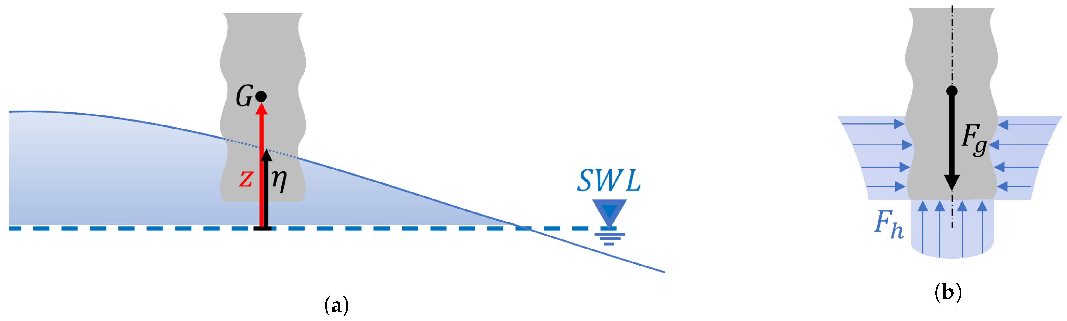
2.1.1. The Hydrostatic Restoring Force

The hydrostatic restoring force equals the difference between the buoyancy force from the fluid and the weight of the WEC:

$$F_s\left(z\right)=\rho gV\left(z\right)-F_g,$$

(5)

where $\rho$ is the density of the sea water, g is the gravitational constant and $V\left(z\right)$ is the submerged volume of the WEC, which increases/decreases as the WEC heaves into/out of the water. At equilibrium, $z=0$, the buoyancy force balances the weight of the WEC, $\rho gV\left(0\right)=F_g$. Therefore, the hydrostatic restoring force equals the weight of the fluid, which is displaced by the change in the submerged WEC volume:

$$F_s\left(z\right)=\rho g\Delta V\left(z\right),$$

(6)

where $\Delta V\left(z\right)=V\left(z\right)-V\left(0\right)$. For a linear hydrodynamic model, the change in the submerged WEC volume is assumed to be linearly proportional to the waterplane area $A_s$ of the WEC’s cross-section at equilibrium:

$$\Delta V\left(z\right)=A_{s}z.$$

(7)

This assumption is strictly true for geometries with constant cross-sections, such as vertical cylinders, and is otherwise approximately true for very small heave displacements from the equilibrium. However, for geometries with non-constant cross-sectional areas, this linearising assumption breaks down with the increase in heave amplitude.

2.1.2. The Wave Radiation Force

The wave radiation is the reaction force due to the radiated wave created by a body moving in the fluid, comprising an inertia term due to the fluid mass surrounding the body that must be accelerated and a resistance term due to the energy carried away by the wave:

$$F_r(\dot{z},\ddot{z},\omega )=-m_a\left(\omega \right)\ddot{z}-c_a\left(\omega \right)\dot{z},$$

(8)

where $m_a\left(\omega \right)$ and $c_a\left(\omega \right)$ are the frequency-dependent added mass and damping coefficients, respectively. The added mass and damping parameters depend on the WEC geometry and the properties of the surrounding fluid.

2.1.3. The Wave Excitation Force

The wave excitation force is the force exerted on a body that is held fixed in the presence of an incident wave. For linear hydrodynamic models, the excitation force is assumed to be linearly proportional to the wave amplitude and is also phase shifted with respect to the position of the wave:

$$F_e(t,\omega )=f_e\left(\omega \right)Hcos(\omega t-{\theta }_e\left(\omega \right)),$$

(9)

where $f_e\left(\omega \right)$ is the excitation force coefficient, and ${\theta }_e\left(\omega \right)$ is the phase angle between the wave and the excitation force. Both of these parameters are frequency-dependent and also depend on the geometry of the WEC and the properties of the surrounding fluid.

2.1.4. The Linear Hydrodynamic Model

Combining the expressions for the three hydrodynamic forces in in Section 2.1.1, Section 2.1.2 and Section 2.1.3 with the equation of motion for the WEC, Equation (3), provides the conventional linear hydrodynamic model used for WEC simulation:

$$\left(m+m_a\left(\omega \right)\right)\ddot{z}+c_a\left(\omega \right)\dot{z}+\rho g{A}_{s}z=f_e\left(\omega \right)Hcos(\omega t-{\theta }_e\left(\omega \right)).$$

(10)

2.2. Analytical Model for Parametric Resonance

Here the linear hydrodynamic model in Section 2.1.4 is modified to more accurately describe the case of a heaving WEC with a non-constant waterplane area. In Section 2.2.1, a nonlinear hydrostatic restoring force is introduced to better represent the actual, rather than linearised, change in the submerged WEC volume as a function of the heave displacement. Section 2.2.2 derives a parametric forcing term by introducing position dependence to the excitation force coefficients. The nonlinear hydrostatic restoring force and parametric excitation terms are incorporated in the conventional hydrodynamic model in Section 2.2.3, which is rearranged to cast it in a form similar to the Mathieu equation.

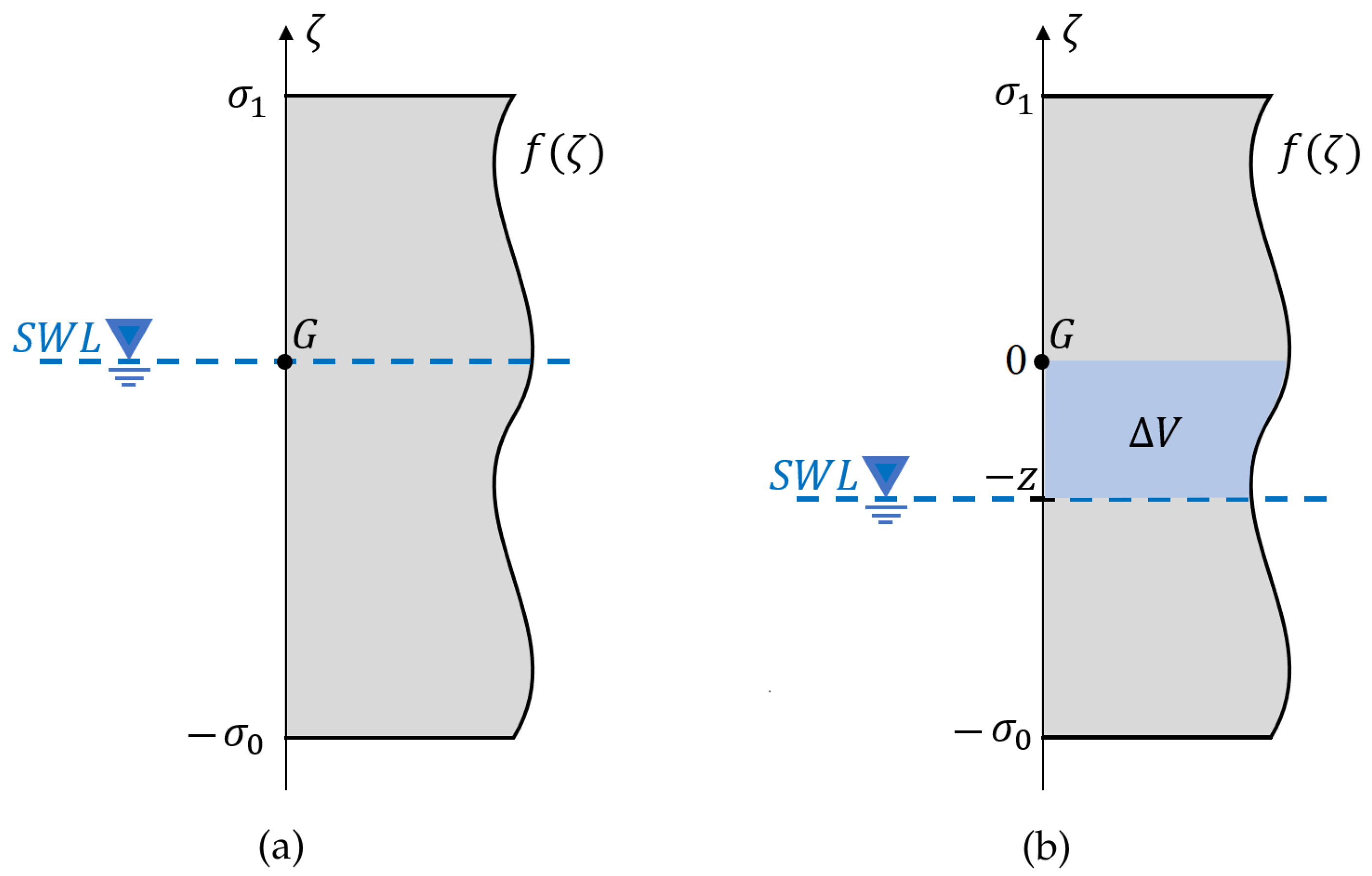
2.2.1. Nonlinear Hydrostatic Restoring Force

The hydrostatic restoring force is proportional to the change in the displaced water volume due to the heave motion of the WEC, $\Delta V\left(z\right)$. Rather than assuming $\Delta V\left(z\right)$ is linearly proportional to the heave motion, as in Equation (7), a nonlinear function can be utilised to more accurately represent $\Delta V\left(z\right)$ in order to increase the fidelity of the hydrostatic restoring force term.

Nonlinear hydrostatic restoring force terms have previously been implemented in WEC models, whereby the restoring force is expressed as a polynomial function of the displacement [93,98,99]. In these models, the polynomial expressions for the restoring force are identified using data of the hydrostatic force versus the WEC displacement, as measured from static tests in the laboratory [98] or CFD-based numerical wave tanks [93,99]. In the present paper, a polynomial expression is instead identified for $\Delta V\left(z\right)$, rather than the hydrostatic force directly, using data generated from an analytical function describing the WEC geometry.

Considering an arbitrary shaped buoy, with a cross-sectional area $A_w\left(\zeta \right)$ that can vary along its vertical axis, $\zeta$. The change in the displaced volume of water due to a heave displacement of z can be written as:

$$\Delta V\left(z\right)={\int }_{-z}^0{A}_w\left(\zeta \right)\mathrm{d}\zeta .$$

(11)

For axisymmetric buoys, Equation (11) can be simplified to:

$$\Delta V\left(z\right)=\pi {\int }_{-z}^0{f}^2\left(\zeta \right)\mathrm{d}\zeta ,$$

(12)

where the axisymmetric geometry of the buoy is defined by the revolution of a generic function $f\left(\zeta \right),\zeta \in [-{\sigma }_0,{\sigma }_1]$, see Figure 2, where the origin of the body fixed coordinate system $\zeta$ is denoted by G, and it is located at the still water level when the buoy is at rest.

The integral expression for $\Delta V\left(z\right)$ in either Equation (11) or (12) can be approximated by using an nth degree polynomial expression, i.e.,

$$\Delta V\left(z\right)\approx \sum _{k=1}^n{c}_k{z}^k,$$

(13)

where the coefficients $c_1,\cdots ,c_n$ can be determined by the least squares method. The hydrostatic restoring force can then be expressed as

$$F_s\left(z\right)=-\rho g\sum _{k=1}^n{c}_k{z}^k.$$

(14)

2.2.2. Parametric Excitation

Here the wave excitation force is recast into a parametric excitation term, which to the authors’ knowledge has not been proposed before. This is achieved by introducing time-varying parameters to the excitation force model (Equation (9)). While the conventional linear hydrodynamic model determines the excitation force coefficient, $f_e\left(\omega \right)$, and phase angle, ${\theta }_e\left(\omega \right)$, based on the wetted surface area of the submerged buoy geometry at equilibrium, the proposed method here determines these two parameters based on the instantaneous heave position. Therefore, rather than being constant, the excitation force coefficient, $f_e(z,\omega )$, and phase angle, ${\theta }_e(z,\omega )$, now depend on the position of the buoy and convert the wave excitation force into a parametric forcing term:

$$F_e(t,\omega )=f_e(z,\omega )Hcos(\omega t-{\theta }_e(z,\omega )).$$

(15)

Similar to the derivation of the nonlinear hydrostatic restoring force in Section 2.2.1, the excitation force coefficient and phase angle can be expressed as a nonlinear function of the heave displacement by fitting polynomial functions to data

$$f_e(z,\omega )=\sum _{k=1}^n{a}_k\left(\omega \right)z^k,{\theta }_e(z,\omega )=\sum _{k=1}^n{b}_k\left(\omega \right)z^k,$$

(16)

where the coefficients $a_1,\dots ,a_n$ and $b_1,\dots ,b_n$ can be determined (e.g., by the least squares method) from a dataset comprising the values of $f_e\left(\omega \right)$ and ${\theta }_e\left(\omega \right)$ for several different submergence levels of the buoy (rather than just at the equilibrium position as is the case for the linear hydrodynamic model). The general form of the wave excitation force then becomes:

$$F_e(t,\omega )=\sum _{k=1}^n{a}_k\left(\omega \right)z^{k}Hcos(\omega t-b_k\left(\omega \right)z^k).$$

(17)

2.2.3. Mathieu Type Equation

Incorporating Equations (14) and (17) into Equation (10), the analytical model for a heaving buoy with a non-constant cross-sectional area is

$$\left(m+m_a\left(\omega \right)\right)\ddot{z}+c_a\left(\omega \right)\dot{z}+\rho g\sum _{k=1}^n{c}_k{z}^k=\sum _{k=1}^n{a}_k\left(\omega \right)z^{k}Hcos(\omega t-b_k\left(\omega \right)z^k).$$

(18)

This can be recast into a Mathieu/Hill-type form

$$\left(m+m_a\left(\omega \right)\right)\ddot{z}+c_a\left(\omega \right)\dot{z}+\sum _{k=1}^n{z}^k\left(\rho g{c}_k+a_k\left(\omega \right)Hcos(\omega t+b_k\left(\omega \right)z^k)\right)=0.$$

(19)

3. Test Case

To evaluate the proposed analytical model, a test case is presented comparing the performance of the model against two other models. First, to investigate the influence of the novel parametric excitation term (introduced in Section 2.2.2), the results of the analytical model are compared against the results from a model that only extends the conventional linear model with a nonlinear hydrostatic restoring force term. Next, the performance of the analytical model is compared and verified against a high-fidelity benchmark produced herein by the NLFK model implemented using an open source toolbox [100]. The WEC geometry is introduced in Section 3.1, and the derivation of the analytical model for this particular geometry is presented in Section 3.2. The nonlinear hydrostatic and NLFK force models and their implementation are detailed in Section 3.3 and Section 3.4, respectively.

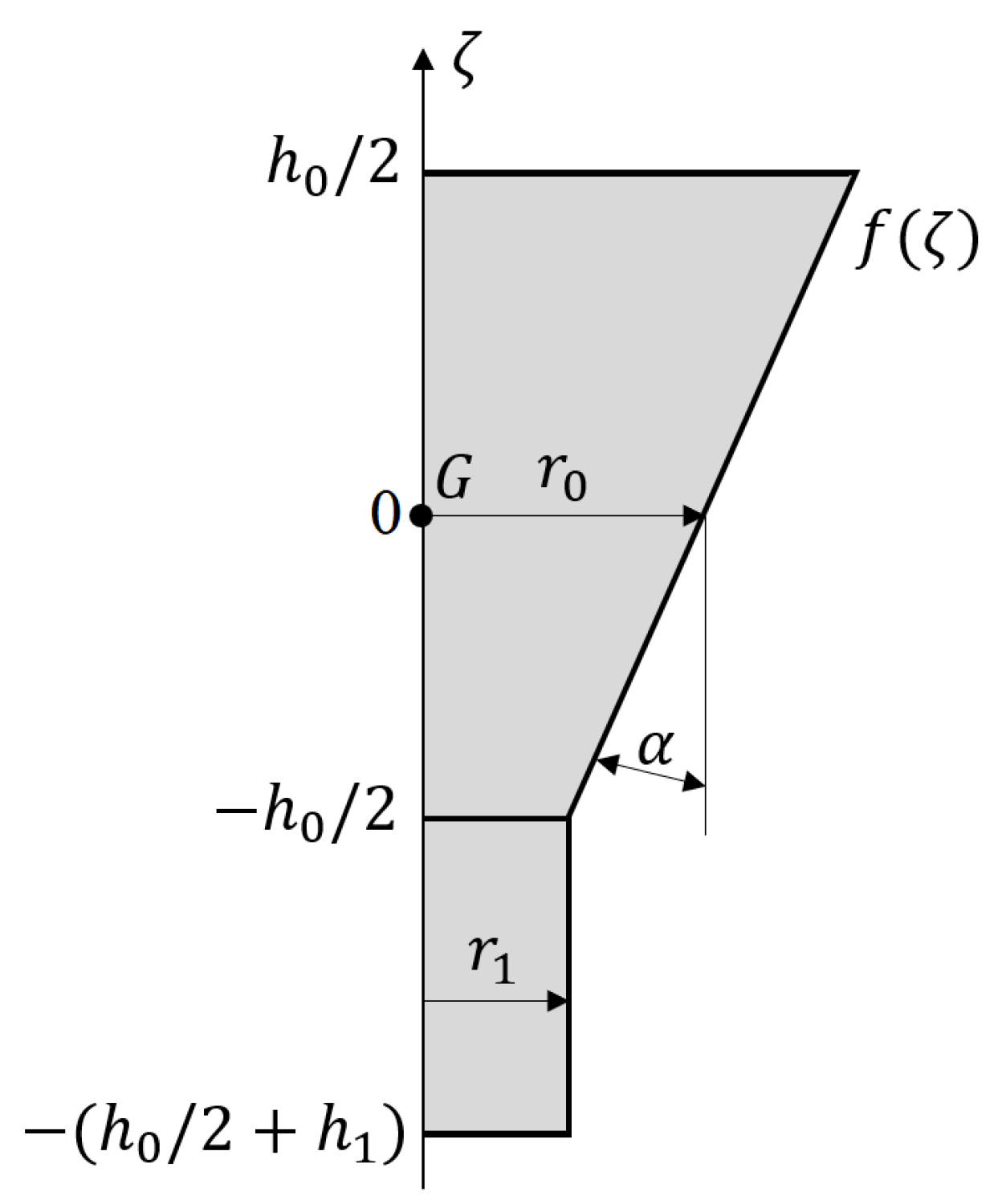
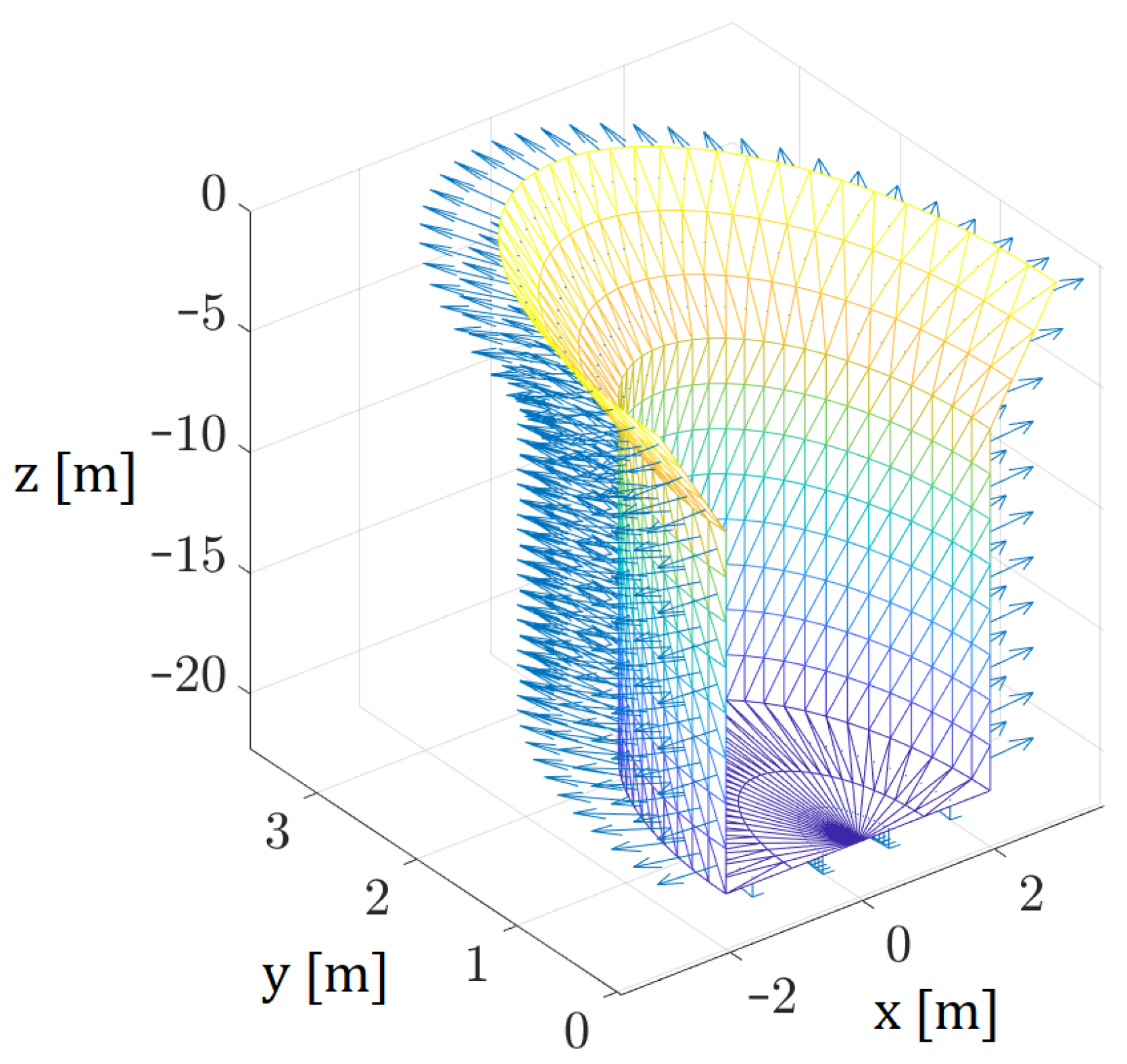
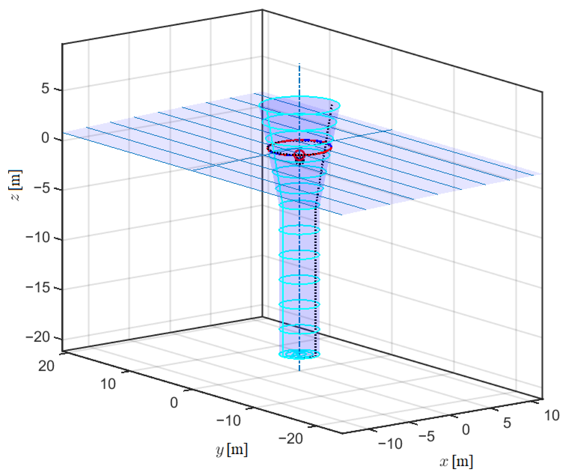
3.1. Test Case Geometry

The test case considers a heaving point absorber WEC with a non-constant waterplane area, as shown in Figure 3, whose geometry comprises a truncated cone-shaped buoy with a cylindrical extension. The parameters of the buoy geometry are listed in

Table 1. Parameters of the test case geometry.

Parameter		Value	Units
Opening angle of the conical part	$\alpha$	11.31	${}^{\circ }$
Radius of the conical part at equilibrium state at still water level	$r_0$	3	$\mathrm{m}$
Half-length of the conical part	$h_0$	5	$\mathrm{m}$
Radius of the cylindrical extension	$r_1$	2	$\mathrm{m}$
Length of the cylindrical extension	$h_1$	15	$\mathrm{m}$

.

The shape of this buoy is defined by

$$f\left(\zeta \right)=\left\{\begin{array}{cc}{r}_1\hfill & \mathrm{if}-(h_0/2+h_1)<\zeta \le -h_0/2,\hfill \\ r_0+\gamma \zeta \hfill & \mathrm{if}-h_0/2<\zeta \le h_0/2,\hfill \\ 0\hfill & \mathrm{otherwise},\hfill \end{array}\right.$$

(20)

where $\gamma =tan\alpha$. To be consistent with Figure 2, we note that for the test case, ${\sigma }_0=h_0/2+h_1$ and ${\sigma }_1=h_0/2$.

3.2. The Analytical Model

The calculation of the parameters in the analytical model (Equation (19)) for the test case WEC geometry is detailed here. Section 3.2.1 describes the calculation of the hydrostatic restoring force parameters, Section 3.2.2 the parametric excitation and Section 3.2.3 the radiation force.

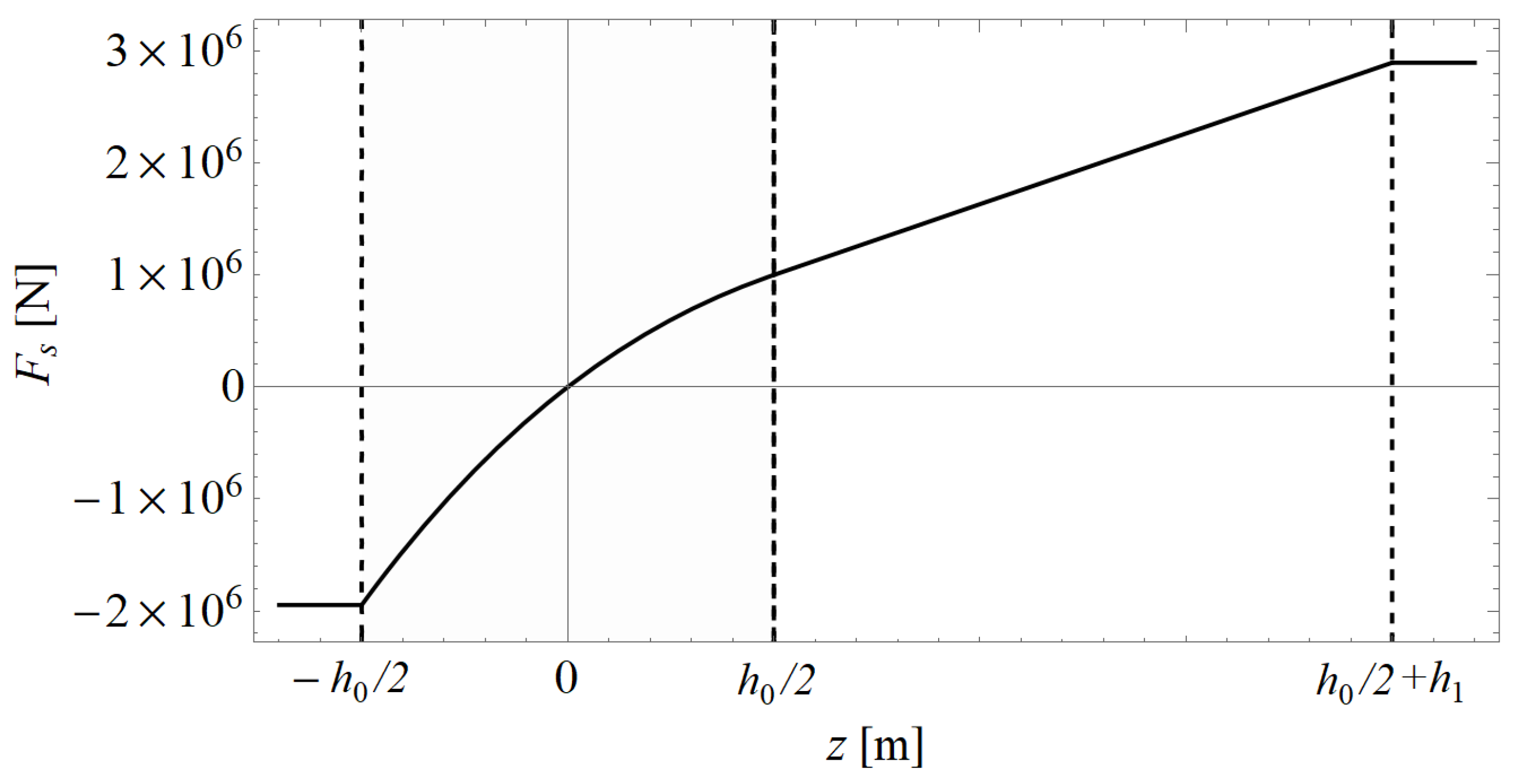
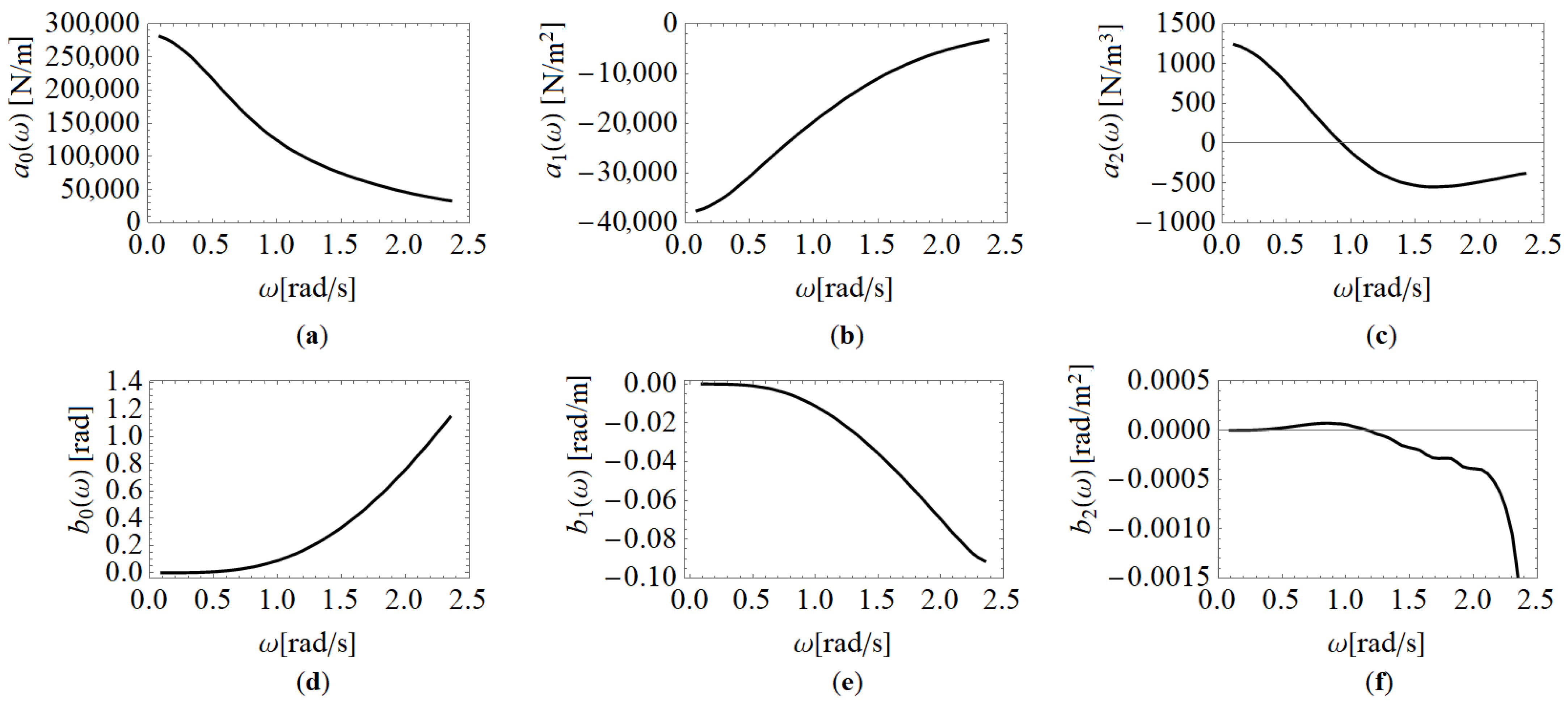
3.2.1. Hydrostatic Restoring Force

To calculate the nonlinear hydrostatic force, the displaced water volume has to be determined. Using Equation (11), the volume of the displaced water due to variations in heave position z can be calculated for the test case geometry. Substituting the displaced water volume into Equation (6), the nonlinear hydrostatic force of the test case geometry can be written as

$$\begin{array}{cc}\hfill F_s\left(z\right)=& -\rho g\Delta V\left(z\right)=-\rho g\pi {\int }_{-z}^0{f}^2\left(\zeta \right)\mathrm{d}\zeta =\hfill \\ \hfill =& \left\{\begin{array}{cc}-\rho g\pi \left(r_0^2(-h_0/2)-\gamma r_0{(-h_0/2)}^2+\frac{1}{3}{\gamma }^2{(-h_0/2)}^3\right),\hfill & \mathrm{if}z\le -h_0/2,\hfill \\ -\rho g\pi \left(r_0^{2}z-\gamma r_0{z}^2+\frac{1}{3}{\gamma }^2{z}^3\right),\hfill & \mathrm{if}-h_0/2<z\le h_0/2,\hfill \\ -\rho g\pi \left(r_0^2(h_0/2)-\gamma r_0{(h_0/2)}^2+\frac{1}{3}{\gamma }^2{(h_0/2)}^3+r_1^2(z-h_0/2)\right),\hfill & \mathrm{if}{h}_0/2<\zeta \le h_0/2+h_1,\hfill \\ -\rho g\pi \left(r_0^2(h_0/2)-\gamma r_0{(h_0/2)}^2+\frac{1}{3}{\gamma }^2{(h_0/2)}^3+r_1^2{h}_1\right),\hfill & \mathrm{if}{h}_0/2+h_1<z.\hfill \end{array}\right.\hfill \end{array}$$

(21)

The water density and the gravitational acceleration were set to $\rho =1025[\mathrm{kg}/{\mathrm{m}}^3]$ and $g=9.806[\mathrm{m}/{\mathrm{s}}^2]$, respectively. The resulting nonlinear hydrostatic force $F_s\left(z\right)$ for the test case geometry is illustrated in Figure 4. The piecewise function of the hydrostatic force has a strong nonlinear characteristic in the $-h_0/2<z\le h_0/2$ domain.

3.2.2. Parametric Excitation

The wave excitation force amplitude and phase coefficients were calculated by the open source code NEMOH [101]. This code is a numerical solver for computation of first-order hydrodynamic coefficients, such as added mass, radiation, damping and excitation forces, in the frequency domain. NEMOH is based on linear free surface potential flow theory with assumptions of an inviscid fluid and an incompressible and irrotational flow. The resulting linear Boundary Value Problem (BVP) for the free surface flow around a body is of first order with assumptions of small motions around the mean position and linearised free surface equations. We enable the simulation of large motions by calculating the hydrodynamic coefficients at numerous buoy submergence levels. The assumption of small motions mean that the calculated hydrodynamic parameters are only accurate in a small displacement range around the submergence level they were calculated. Therefore, we allow the parameters in the model to change based on the displacement, so they match the values corresponding to the instantaneous submergence level during the simulation.

In order to solve the linear BVP, panel methods are applied in NEMOH. For the present test case, the buoy geometry was discretised using 445 panels and 1120 nodes. The mesh created for NEMOH is illustrated in Figure 5. The mesh independence was checked by using two other meshes with 230 and 880 panels.

The excitation amplitude and phase were calculated for $\omega \in [0.05,2.4]$ [rad/s] with a step size of $\delta \omega =0.05$ [rad/s] and at 11 different buoy submergence levels where the position of the buoy is vertically translated by $z\in \{-5,-4,-3,-2,-1,0,1,2,3,4,5\}$ [m]. Figure 6 illustrates the parameters of the wave excitation force $(f_e(z,\omega ),{\theta }_e(z,\omega ))$ for the test case buoy.

For this current test case, second-order polynomials are employed to approximate the wave excitation amplitude and phase as a function of the buoy position for each frequency, i.e.,

$$f_e(z,\omega )=a_2\left(\omega \right)z^2+a_1\left(\omega \right)z+a_0\left(\omega \right),{\theta }_e(z,\omega )=b_2\left(\omega \right)z^2+b_1\left(\omega \right)z+b_0\left(\omega \right),$$

(22)

where the frequency-dependent coefficients $a_0\left(\omega \right),a_1\left(\omega \right),a_2\left(\omega \right),b_0\left(\omega \right),b_1\left(\omega \right),b_2\left(\omega \right)$ are least-square fitted on the NEMOH data. The coefficients as the function of the wave frequency $\omega$ are illustrated in Figure 7.

The accuracy of the fitted wave excitation amplitude $f_e(z,\omega )$ and phase ${\theta }_e(z,\omega )$ are illustrated in Figure 8, where the continuous line denotes the fitted curve, while the dots are the data calculated by NEMOH.

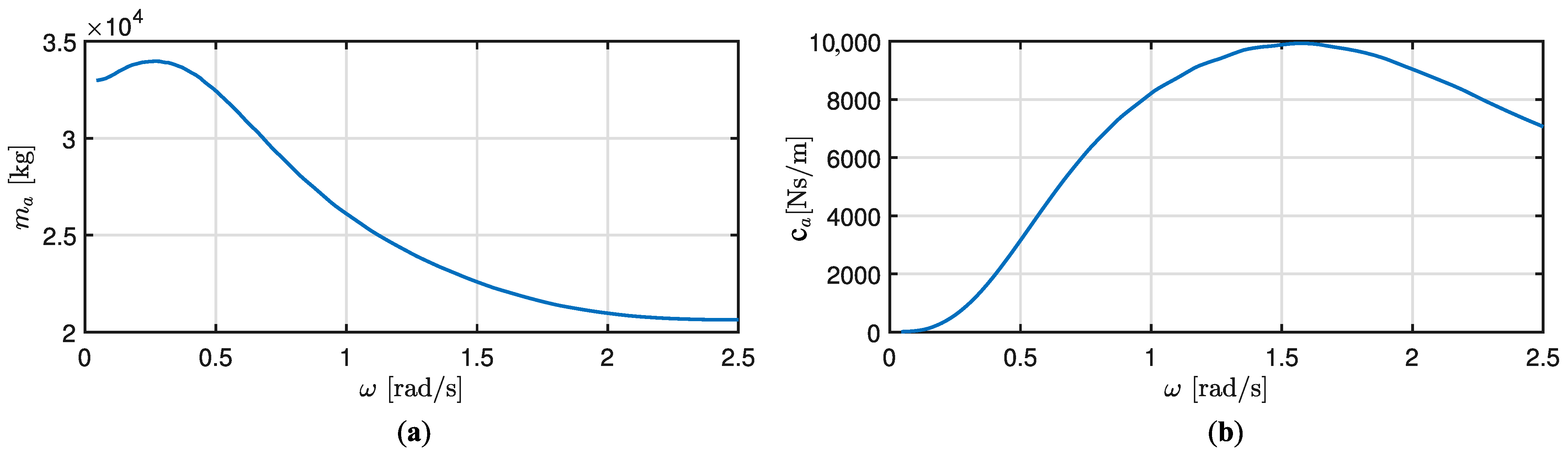
3.2.3. Wave Radiation Force

The added mass $m_a\left(\omega \right)$ and damping $c_a\left(\omega \right)$ were also calculated using NEMOH for the $z=0$ buoy position (as they are considered here as independent of the position). Figure 9 illustrates the added mass and radiation damping coefficients as a function of the wave frequency $\omega$.

3.3. The Nonlinear Hydrostatic Restoring Force Model

The nonlinear hydrostatic restoring force model extends the conventional linear hydrodynamic model (Equation (10)) with the nonlinear restoring force described in Section 2.2.1:

$$\left(m+m_a\left(\omega \right)\right)\ddot{z}+c_a\left(\omega \right)\dot{z}+\rho g\sum _{k=1}^n{c}_k{z}^k=f_e\left(\omega \right)Hcos(\omega t-{\theta }_e\left(\omega \right)).$$

(23)

This type of nonlinear hydrodynamic model has previously been utilised for WECs with position-varying waterplane areas [93,98,99] but does not enable parametric resonance to be captured. The parameters for the hydrostatic restoring force and the radiation force are the same as calculated in Section 3.2.1 and Section 3.2.3, respectively. The parameters for the exciation force are the same as calculated for the equilibrium postion ($z=0$) in Section 3.2.2.

3.4. The Nonlinear Froude–Krylov Force Model

In this section, we describe the NLFK model used for the code-to-code verification of the analytical model developed in this paper. The hydrodynamic force in the NLFK is considered in the following way:

$$F_h(z,\dot{z},\ddot{z},t,\omega )=F_{F{K}_z}\left(z,t,\omega \right)+F_r(\dot{z},\ddot{z},\omega ),$$

(24)

where $F_{F{K}_z}\left(z,t,\omega \right)$ is the Froude–Krylov force acting in z-direction, and $F_r(\dot{z},\ddot{z},\omega )$ is the linear radiation force (see Equation (8)). The resulting equation of motion is

$$\left(m+m_a\left(\omega \right)\right)\ddot{z}+c_a\left(\omega \right)\dot{z}=F_{F{K}_z}\left(z,t,\omega \right).$$

(25)

Froude–Krylov (FK) forces correspond to the integral of the pressure (static and dynamic) of the undisturbed incident wave field over the wetted surface of the device. Such a pressure is defined, according to linear Airy’s theory, with the application of Wheeler stretching [102], as:

$$p(x,z,t)=p_{st}+p_{dy}=-\rho gz+\rho gHcos(\omega t-kx)\frac{cosh\left(k\left(z^{\prime }+h\right)\right)}{cosh\left(kh\right)},$$

(26)

where $p_{st}$ and $p_{dy}$ are the static and dynamic pressure, respectively. The variable $z^{\prime }$ is the change of coordinates required by Wheeler stretching in order to eliminate the free surface boundary condition error: $z^{\prime }=h\frac{z+h}{\overline{\eta }+h}-h$, where $\overline{\eta }$ is an approximation of the free surface, computed at the center of gravity. The FK force can be divided into the static and dynamic FK forces

$${\mathbf{F}}_{FK}={\mathbf{F}}_{F{K}_{st}}+{\mathbf{F}}_{F{K}_{dy}}.$$

(27)

The static FK force is defined as:

$${\mathbf{F}}_{F{K}_{st}}={\mathbf{F}}_g+\underset{S_w}{\int \int }{p}_{st}\mathbf{n}\mathrm{d}S,$$

(28)

where ${\mathbf{F}}_g={(0,0,-mg)}^T$ is the weight, $S_w$ the instantaneous wetted surface and $\mathbf{n}$ the unity vector normal to the surface. The dynamic FK force is similarly defined as the surface integral of the dynamic pressure:

$${\mathbf{F}}_{F{K}_{dy}}=\underset{S_w}{\int \int }{p}_{dy}\mathbf{n}\mathrm{d}S.$$

(29)

To calculate the Froude–Krylov force $F_{F{K}_z}$ in the time domain simulations, the open-source NLFK4ALL MATLAB toolbox developed by Giorgi [100,103] was utilised. The Froude–Krylov force $F_{F{K}_z}\left(z,t,\omega \right)$ was calculated every time step using NLFK4ALL toolbox, and the equation of motion was integrated using the fourth order Runge–Kutta method. To choose the proper time step for the integration, we checked time sensitivity of the solution on the time step, see Figure 10.

To reduce the simulation time and keep the proper accuracy, $\Delta t=0.002$ [s] was chosen as the simulation time step. Figure 11 illustrates a rendering of the test case geometry provided within the NLFK4ALL toolbox.

4. Results

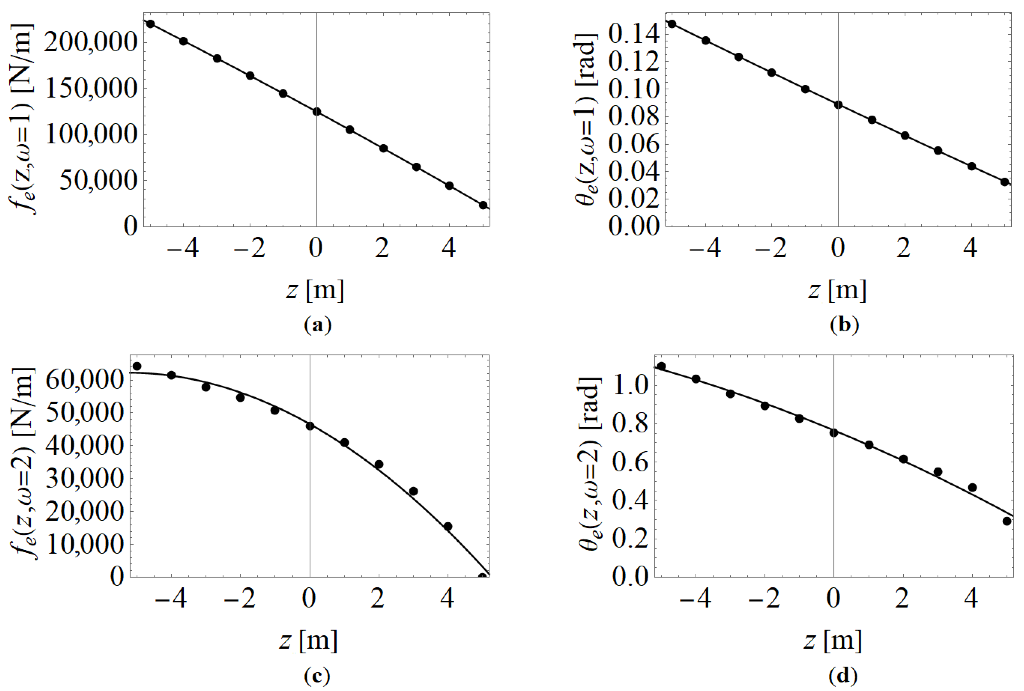
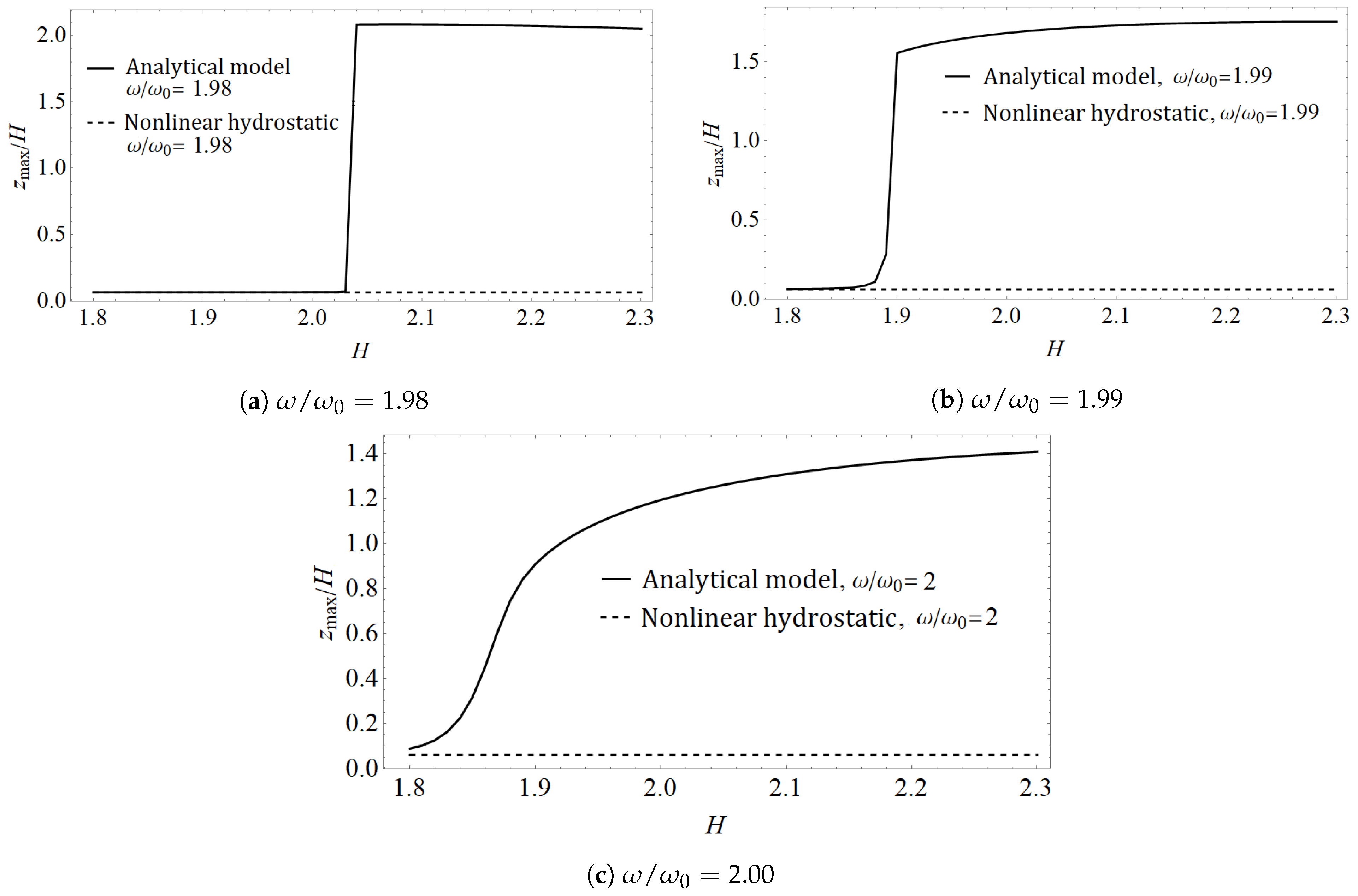
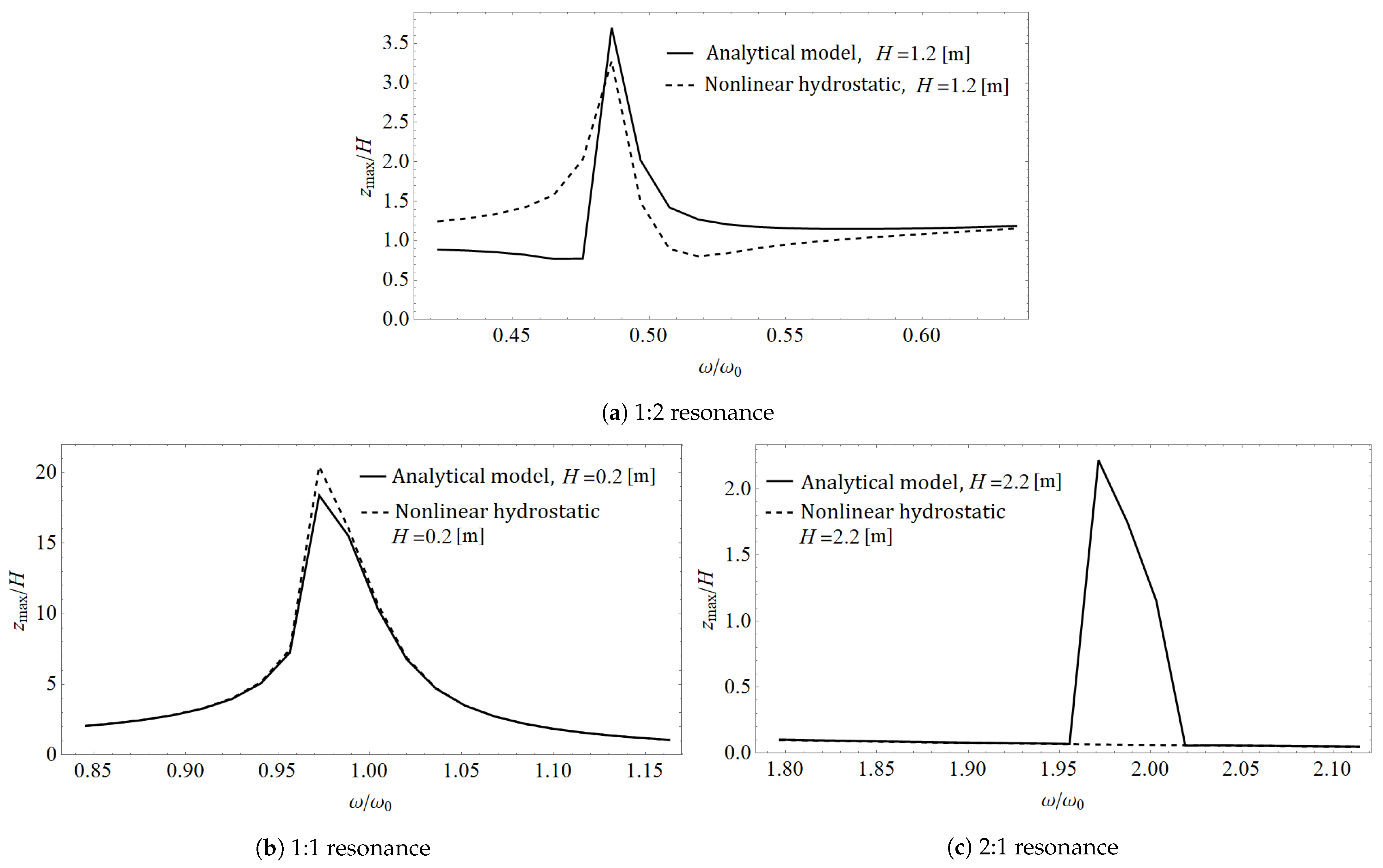
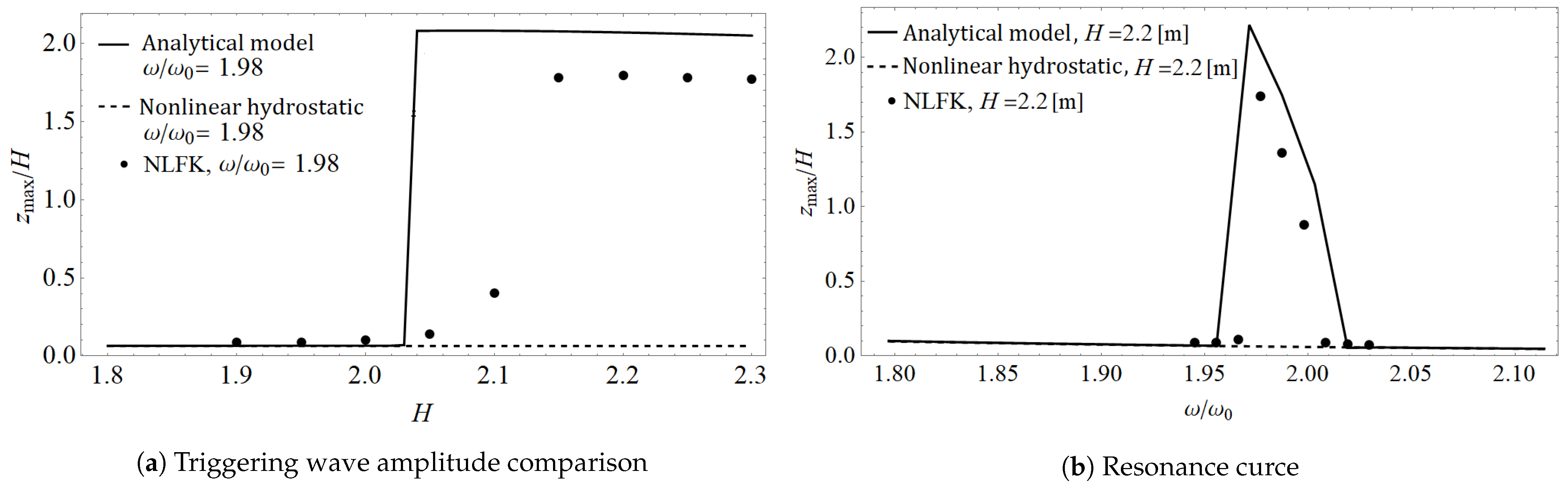
4.1. Comparison against Nonlinear Hydrostatic Restoring Force Model

Parametric resonance is expected to occur for input waves with a frequency twice the buoy’s natural frequency and with amplitudes above a certain threshold. To examine the ability of the analytical model to capture parametric resonance, numerous simulations were performed at frequencies close to twice the buoy’s natural frequency for a range of wave heights. The buoy’s natural frequency was measured from free decay experiments (see Section 4.2) and equals ${\omega }_0=0.944[\mathrm{rad}/\mathrm{s}]$.

Figure 12 shows the buoy steady-state oscillation amplitude, normalised against the wave amplitude, $z_{max}/H$, as a function of the wave amplitude H. For a linear system, normalising the output by the input amplitude results in a constant as a function of the input amplitude. Therefore, due to the normalisation in Figure 12, any deviation from a constant response highlights the nonlinearity in the output and the threshold wave amplitude where this nonlinearity manifests. The results are shown for three different wave frequencies $\omega \in \{1.87,1.88,1.89\}$ [rad/s] in Figure 12a, Figure 12b and Figure 12c, respectively. The solid line denotes the oscillation amplitudes if we apply the new analytical parametric wave excitation model, while the dashed line is the oscillation amplitudes in the case of the simpler nonlinear hydrostatic restoring force model. The results show the analytical model is able to capture parametric resonance, signified by a large dramatic increase in the normalised oscillation amplitude when the wave amplitude reaches a certain threshold, whereas the nonlinear hydrostatic restoring force model is not able to capture this. Comparing Figure 12a–c shows that the threshold wave amplitude to trigger parametric resonance decreases as the wave frequency approaches twice the buoy’s natural frequency ($\omega /{\omega }_0=2$).

The results in Figure 13 show the normalised steady-state oscillation amplitude as a function of the input wave frequency, considering frequencies near, (a) half, (b) equal and (c) double the buoy’s natural frequency. These frequencies correspond to the so-called (a) 1:2, (b) 1:1 and (c) 2:1 resonances, respectively. Note that the wave amplitude is constant for each frequency within a particular graph but differs between graphs due to the different threshold amplitudes required to trigger the 1:2 and 2:1 resonances (seen in more detail in Section 4.3). However, the oscillation amplitudes are normalised against the wave amplitude to allow a comparison between graphs. The analytical and nonlinear hydrostatic restoring force models are seen to give similar results in the vicinity of the 1:2 and 1:1 resonance frequencies. However, only the analytical model is able to capture the parametric resonance in the vicinity of the 2:1 resonance frequency.

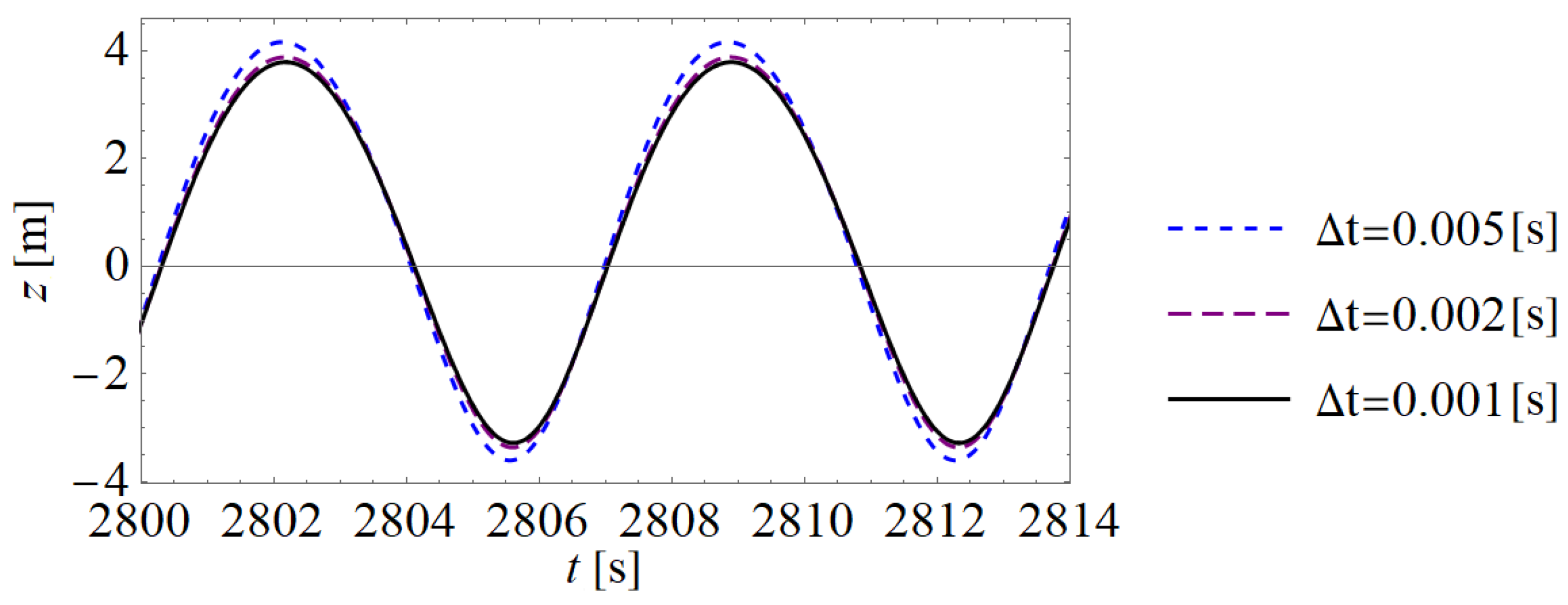
4.2. Code-to-Code Verification against a NLFK Force Model

First, we compared the free response (no wave conditions) of the two models, see Figure 14a. We started the simulation from an initial displacement $z(t=0)=4$ [m], and the two models gave almost identical results. A small difference in the frequency of oscillations can be observed. This can be shown on the power spectral density plot of time series, see Figure 14b.

Secondly, the response of the two models to the parametric was investigated, considering a range of input wave series in the frequency range near the 2:1 resonance. The major difference between the two models is the required computational time to run the simulation. Each input wave series is 3000 [s] in duration, requiring 2 [s] of computational time for the analytical model, compared to 14,000 [s] for the NLFK model (the simulation was run on a Core i7 7700HQ processor). This highlights a significant advantage of the analytical model, being 3–4 orders of magnitude faster than the NLFK model.

Figure 15 shows an example of the predicted heave motions of the buoy for wave amplitude $H=2.2$ [m] and frequency $\omega =1.87$ [rad/s]. The oscillation amplitude grows slightly faster and larger for the analytical model compared to the NLFK model. In addition, there appears to be a small phase difference between the response of the two models.

Figure 16a shows the normalised oscillation amplitudes, $z_{max}/H$, for a range of wave amplitudes at a frequency of $\omega =1.98{\omega }_0$, comparing the results of the analytical, nonlinear hydrostatic and NLFK models. Due to the computational requirements, the NLFK results are obtained for less different wave amplitudes than the other two computationally efficient models. The results from the analytical model agree reasonably well with the NLFK model results. The main difference is in the oscillation amplitudes, which are approximately $15\%$ higher in the analytical model compared to the NLFK model. Figure 16b illustrates the normalised oscillation amplitudes $z_{max}/H$ for varying wave frequencies in the vicinity of the 2:1 resonance for a fixed wave amplitude of 2.2 [m]. Once again, the oscillation amplitudes are slightly higher for the analytical model. In addition, the range of frequencies for which parametric resonance occurs is slightly larger for the analytical model.

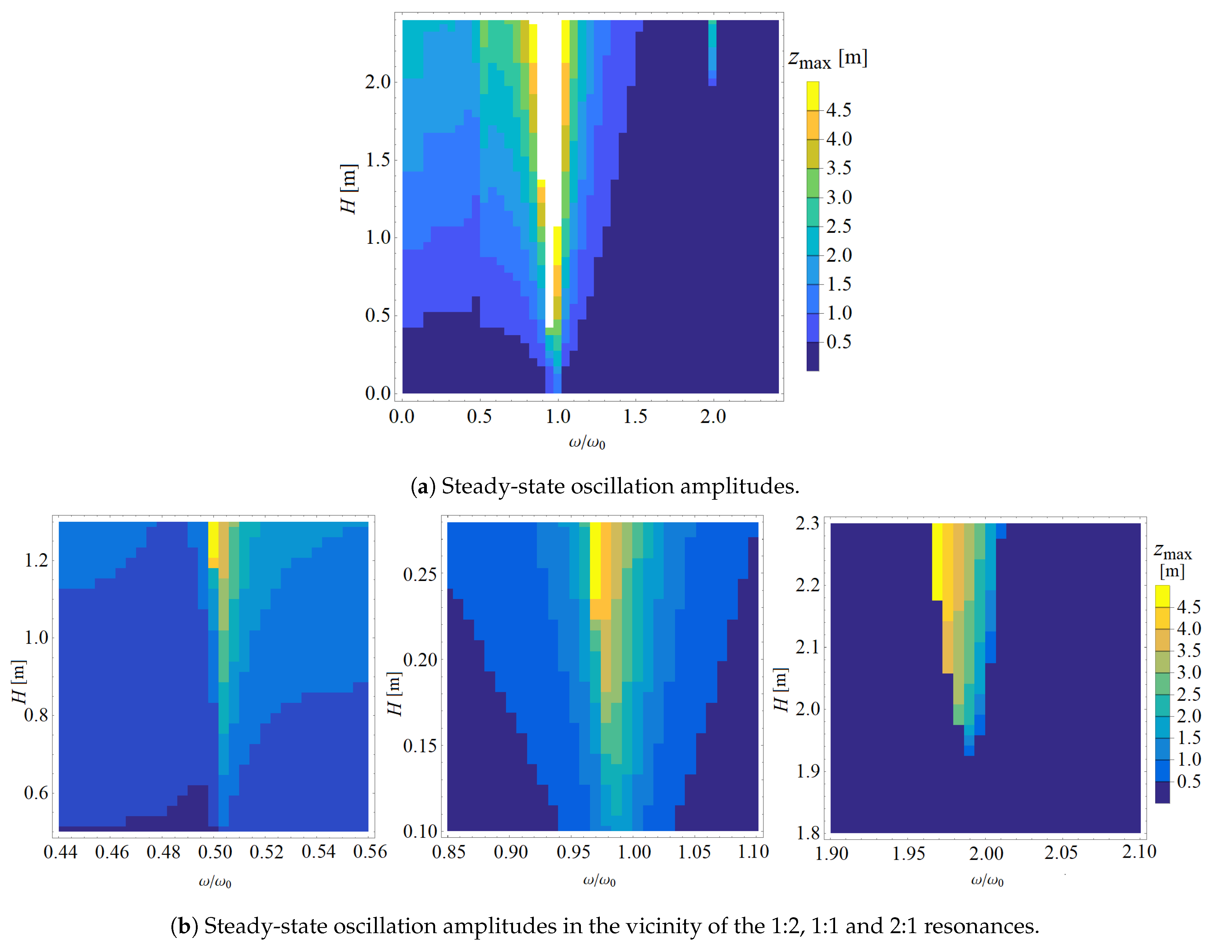
4.3. Two-Parameter Analysis

The simulation speed of the new model with parametric excitation allows us to make multi-parameter investigations. In this subsection, the effect of the wave frequency, together with the amplitude on the buoy dynamics, is analysed. Figure 17 illustrates the buoy steady-state oscillation amplitudes $z_{max}$ as a function of the wave amplitude H and frequency ration $\omega /{\omega }_0$. From Figure 17, we can conclude that the classical 1:1 resonance provides the largest steady-state oscillation amplitude for a given wave amplitude. To trigger the 2:1 resonance, large wave amplitudes are required. Below $H=1.92\left[\mathrm{m}\right]$, the radiation damping mitigates the occurrence of parametric resonance. Indeed, the amount of damping in the system dictates the threshold at which parametric resonance occurs; therefore, an accurate measure of the total damping in the system is vital. The current model built upon the conventional linear hydrodynamic model that assumes an inviscid fluid and therefore neglects any type of viscous damping. However, the effect of viscosity becomes less negligible as the size of the buoy decreases, its velocity increases and/or its geometry become less streamlined. As such, a viscous damping term can be added to this model whose parameters can be identified from CFD simulations [104,105,106,107,108,109,110,111,112]. In addition, for the case of a WEC, the power take-off (PTO) will apply damping in order to extract energy. Therefore, compared to regular 1:1 resonance, the potential of parametric resonance for the present test case (whose geometry was chosen arbitrarily) seems limited. The efficient analytical model developed in this paper will allow future work to explore the vast space of possible geometries to examine the potential of exploiting parametric resonance and finding the appropriate relationships between the wave climates and the buoy dimensions.

5. Conclusions

In this paper, an analytical model for a heaving buoy with a position-varying waterplane area in monochromatic waves is introduced. The target application of the mathematical model is to evaluate the ability of heaving wave energy converters to leverage large amplitude oscillations triggered by the occurrence of parametric resonance due to a position-varying waterplane area. The introduced model extends the capability of current analytical models to be able to capture the occurrence of heave-to-heave Mathieu instabilities using an efficient nonlinear parametrically excited differential equation. The parametric excitation is captured by including position dependence to the excitation force parameters, which is achieved by fitting position-dependent functions (such as polynomials) to the excitation force coefficients calculated for various levels of buoy submergence. The performance of the model efficiently and accurately captures parametric resonance, as verified by a comparison against the results from a nonlinear Froude–Krylov force model, which numerically calculates the forces on the buoy at each time step based on the evolving wetted surface area. The introduced model is demonstrated to perform simulations in monochromatic waves nearly four orders of magnitude faster than the nonlinear Froude–Krylov force model simulations with comparable accuracy. The performance of the model is also compared against an analytical model that only considers the nonlinear effect of the position-varying waterplane area on the restoring force term rather than both the restoring and excitation force terms as the introduced model does. The results show that by only including the nonlinear restoring force term, the model is only able to capture the 1:2 and 1:1 resonances but is unable to capture the 2:1 resonance like the introduced analytical model and the nonlinear Froude–Krylov models can. In addition to the tremendous computational efficiency, by enabling many different WEC parameters to be evaluated using a brute force approach, the introduced model also allows analytical investigation techniques, such as perturbation or harmonic balance methods, to be utilised. These methods will be employed in future work to optimise the geometric design of a heaving WEC to exploit parametric resonance for increased power capture.

References

1. Antonio, F.d.O. Wave energy utilization: A review of the technologies. Renew. Sustain. Energy Rev. 2010, 14, 899–918. [Google Scholar]
2. Aderinto, T.; Li, H. Ocean wave energy converters: Status and challenges. Energies 2018, 11, 1250. [Google Scholar] [CrossRef] [Green Version]
3. Fossen, T.; Nijmeijer, H. Parametric Resonance in Dynamical Systems; Springer: Berlin/Heidelberg, Germany, 2011. [Google Scholar]
4. Falnes, J. Ocean Waves and Oscillating Systems; Cambridge University Press: Cambridge, UK, 2002. [Google Scholar]
5. Folley, M. Numerical Modelling of Wave Energy Converters: State-of-the-Art Techniques for Single Devices and Arrays; Academic Press: Cambridge, MA, USA, 2016. [Google Scholar]
6. Davidson, J.; Costello, R. Efficient nonlinear hydrodynamic models for wave energy converter design—A scoping study. J. Mar. Sci. Eng. 2020, 8, 35. [Google Scholar] [CrossRef] [Green Version]
7. Arvin, H.; Tang, Y.Q.; Nadooshan, A.A. Dynamic stability in principal parametric resonance of rotating beams: Method of multiple scales versus differential quadrature method. Int. J. Non-Linear Mech. 2016, 85, 118–125. [Google Scholar] [CrossRef]
8. Verhulst, F. Perturbation Analysis of Parametric Resonance. Encycl. Complex. Syst. Sci. 2009, 113, 6625–6639. [Google Scholar]
9. Nayfeh, A.; Zavodney, L.D. The response of two-degree-of-freedom systems with quadratic non-linearities to a combination parametric resonance. J. Sound Vib. 1986, 107, 329–350. [Google Scholar] [CrossRef]
10. Warminski, J.; Kecik, K. Instabilities in the main parametric resonance area of a mechanical system with a pendulum. J. Sound Vib. 2009, 322, 612–628. [Google Scholar] [CrossRef]
11. Rand, R.; Barcilon, A.; Morrison, T. Parametric resonance of Hopf bifurcation. Nonlinear Dyn. 2005, 39, 411–421. [Google Scholar] [CrossRef] [Green Version]
12. Son, I.S.; Uchiyama, Y.; Lacarbonara, W.; Yabuno, H. versdsfsfsf. Nonlinear Dyn. 2008, 53, 129–138. [Google Scholar] [CrossRef]
13. Froude, W. On the Rolling of Ships; Institution of Naval Architects: London, UK, 1861. [Google Scholar]
14. Nayfeh, A.H.; Mook, D.T.; Marshall, L.R. Nonlinear coupling of pitch and roll modes in ship motions. J. Hydronautics 1973, 7, 145–152. [Google Scholar] [CrossRef]
15. Neves, M.A.; Rodriguez, C.A. On unstable ship motions resulting from strong non-linear coupling. Ocean Eng. 2006, 33, 1853–1883. [Google Scholar] [CrossRef]
16. Galeazzi, R. Autonomous Supervision and Control of Parametric Roll Resonance. Ph.D. Thesis, Technical University of Denmark, Department of Naval Architecture and Offshore Engineering, Lyngby, Denmark, 2009. [Google Scholar]
17. Shigunov, V.; El Moctar, O.; Rathje, H.; Germanischer Lloyd, A. Conditions of parametric rolling. In Proceedings of the 10th International Conference on Stability of Ships and Ocean Vehicles, St. Petersburg, Russia, 22–26 June 2009. [Google Scholar]
18. Moideen, H.; Falzarano, J. A critical assessment of ship parametric roll analysis. In Proceedings of the 11th International Ship Stability Workshop (ISSW), Wageningen, The Netherlands, 21–23 June 2010; pp. 21–23. [Google Scholar]
19. Dern, J.C. Unstable motion of free spar buoys in waves. In Proceedings of the 9th Symposium on Naval Hydrodynamics, ONR, Paris, France, 20–25 August 1972. [Google Scholar]
20. Koo, B.; Kim, M.; Randall, R. Mathieu instability of a spar platform with mooring and risers. Ocean Eng. 2004, 31, 2175–2208. [Google Scholar] [CrossRef]
21. Neves, M.A.; Sphaier, S.H.; Mattoso, B.M.; Rodriguez, C.A.; Santos, A.L.; Vileti, V.L.; Torres, F. On the occurrence of Mathieu instabilities of vertical cylinders. In Proceedings of the 27th International Conference on Offshore Mechanics and Arctic Engineering, Estoril, Portugal, 15–20 June 2008. [Google Scholar]
22. Li, B.B.; Ou, J.P.; Teng, B. Numerical investigation of damping effects on coupled heave and pitch motion of an innovative deep draft multi-spar. J. Mar. Sci. Technol. 2011, 19, 231–244. [Google Scholar] [CrossRef]
23. Jang, H.; Kim, M. Mathieu instability of Arctic Spar by nonlinear time-domain simulations. Ocean Eng. 2019, 176, 31–45. [Google Scholar] [CrossRef]
24. Haslum, H.; Faltinsen, O. Alternative shape of spar platforms for use in hostile areas. In Proceedings of the Offshore Technology Conference, Houston, TX, USA, 3–6 May 1999. [Google Scholar]
25. Rho, J.B.; Choi, H.S.; Shin, H.S.; Park, I.K. A study on Mathieu-type instability of conventional spar platform in regular waves. Int. J. Offshore Polar Eng. 2005, 15, 104–108. [Google Scholar]
26. Umeda, N.; Hashimoto, H.; Minegaki, S.; Matsuda, A. An investigation of different methods for the prevention of parametric rolling. J. Mar. Sci. Technol. 2008, 13, 16–23. [Google Scholar] [CrossRef]
27. Galeazzi, R.; Pettersen, K.Y. Controlling Parametric Resonance: Induction and Stabilization of Unstable Motions. In Parametric Resonance in Dynamical Systems; Fossen, T.I., Nijmeijer, H., Eds.; Springer: Berlin/Heidelberg, Germany, 2012; pp. 305–327. [Google Scholar]
28. Yang, H.; Xu, P. Effect of hull geometry on parametric resonances of spar in irregular waves. Ocean Eng. 2015, 99, 14–22. [Google Scholar] [CrossRef]
29. Sheng, W.; Flannery, B.; Lewis, A.; Alcorn, R. Experimental studies of a floating cylindrical OWC WEC. In Proceedings of the ASME 2012 31st International Conference on Ocean, Offshore and Arctic Engineering, Rio de Janeiro, Brazil, 1–6 July 2012. [Google Scholar]
30. Gomes, R.; Henriques, J.; Gato, L.; Falcao, A. Testing of a small-scale floating OWC model in a wave flume. In Proceedings of the International Conference on Ocean Energy, Dublin, Ireland, 17–19 October 2012; pp. 1–7. [Google Scholar]
31. Gomes, R.; Henriques, J.; Gato, L.; Falcão, A.d.O. Wave channel tests of a slack-moored floating oscillating water column in regular waves. In Proceedings of the 11th European Wave and Tidal Energy Conference, Nantes, France, 6–11 September 2015; pp. 6–11. [Google Scholar]
32. Beatty, S.J.; Roy, A.; Bubbar, K.; Ortiz, J.; Buckham, B.J.; Wild, P.; Stienke, D.; Nicoll, R. Experimental and numerical simulations of moored self-reacting point absorber wave energy converters. In Proceedings of the Twenty-fifth International Ocean and Polar Engineering Conference, Kona, HI, USA, 21–26 June 2015. [Google Scholar]
33. Gomes, R.; Henriques, J.; Gato, L.; Falcão, A. Experimental Tests of a 1: 16th-Scale Model of the Spar-Buoy OWC in a Large Scale Wave Flume in Regular Waves. In Proceedings of the ASME 2018 37th International Conference on Ocean, Offshore and Arctic Engineering, Madrid, Spain, 1–22 June 2018; American Society of Mechanical Engineers Digital Collection: New York, NY, USA, 2018. [Google Scholar]
34. Kurniawan, A.; Grassow, M.; Ferri, F. Numerical modelling and wave tank testing of a self-reacting two-body wave energy device. In Ships and Offshore Structures; Taylor and Francis Group: London, UK, 2019; pp. 1–13. [Google Scholar]
35. Gomes, R.; Henriques, J.; Gato, L.; Falcão, A. Time-domain simulation of a slack-moored floating oscillating water column and validation with physical model tests. Renew. Energy 2020, 149, 165–180. [Google Scholar] [CrossRef]
36. Gomes, R.; Malvar Ferreira, J.; Ribeiro e Silva, S.; Henriques, J.; Gato, L. An experimental study on the reduction of the dynamic instability in the oscillating water column spar buoy. In Proceedings of the 12th European Wave and Tidal Energy Conference, Cork, Ireland, 27 August–1 September 2017. [Google Scholar]
37. Ortiz, J.P. The Influence of Mooring Dynamics on the Performance of Self Reacting Point Absorbers. Master’s Thesis, University of Victoria, Victoria, BC, Canada, 2016. [Google Scholar]
38. Gomes, R.; Henriques, J.; Gato, L.; Falcao, A. An upgraded model for the design of spar-type floating oscillating water column devices. In Proceedings of the 13th European Wave and Tidal Energy Conference, Napoli, Italy, 1–6 September 2019. [Google Scholar]
39. Villegas, C.; van der Schaaf, H. Implementation of a pitch stability control for a wave energy converter. In Proceedings of the 10th European Wave and Tidal Energy Conference, Southampton, UK, 5–9 September 2011. [Google Scholar]
40. Maloney, P. Performance Assessment of a 3-Body Self-Reacting Point Absorber Type Wave Energy Converter. Master’s Thesis, University of Victoria, Victoria, BC, Canada, 2019. [Google Scholar]
41. Davidson, J.; Gomes, R.; Galeazzi, R.; Henriques, J. Blowing the Top on Parametric Resonance—Relief Valve Control for the Stabiliation of an OWC Spar Buoy. In Proceedings of the ASME 2020 39th International Conference on Ocean, Offshore and Arctic Engineering, Online. 3–7 August 2020; Available online: https://asmedigitalcollection.asme.org/OMAE/proceedings-abstract/OMAE2020/84416/V009T09A033/1093150 (accessed on 18 October 2021).
42. Davidson, J.; Henriques, J.C.; Gomes, R.P.; Galeazzi, R. Opening the air-chamber of an oscillating water column spar buoy wave energy converter to avoid parametric resonance. IET Rene. Power Gener. 2021, 1–17. [Google Scholar] [CrossRef]
43. Davidson, J.; Kalmár-Nagy, T. A Real-Time Detection System for the Onset of Parametric Resonance in Wave Energy Converters. J. Mar. Sci. Eng. 2020, 8, 819. [Google Scholar] [CrossRef]
44. Abdelkhalik, O.; Zou, S.; Robinett, R.; Bacelli, G.; Wilson, D.; Coe, R. Control of three degrees-of-freedom wave energy converters using pseudo-spectral methods. J. Dyn. Syst. Meas. Control 2018, 140, 074501. [Google Scholar] [CrossRef]
45. Zou, S.; Abdelkhalik, O.; Robinett, R.; Korde, U.; Bacelli, G.; Wilson, D.; Coe, R. Model Predictive Control of parametric excited pitch-surge modes in wave energy converters. Int. J. Mar. Energy 2017, 19, 32–46. [Google Scholar] [CrossRef] [Green Version]
46. Abdelkhalik, O.; Zou, S. Time-varying linear quadratic gaussian optimal control for three-degree-of-freedom wave energy converters. In Proceedings of the European Wave and Tidal Energy Conference, College Cork, Ireland, 27 August–1 September 2017. [Google Scholar]
47. Zou, S.; Abdelkhalik, O. Time-varying linear quadratic Gaussian optimal control for three-degree-of-freedom wave energy converters. Renew. Energy 2020, 149, 217–225. [Google Scholar] [CrossRef]
48. Orazov, B.; O’Reilly, O.; Savaş, Ö. On the dynamics of a novel ocean wave energy converter. J. Sound Vib. 2010, 329, 5058–5069. [Google Scholar] [CrossRef]
49. Orazov, B. A Novel Excitation Scheme for an Ocean Wave Energy Converter. Ph.D. Thesis, UC Berkeley, Berkeley, CA, USA, 2011. [Google Scholar]
50. Orazov, B.; O’Reilly, O.M.; Zhou, X. On forced oscillations of a simple model for a novel wave energy converter. Nonlinear Dyn. 2012, 67, 1135–1146. [Google Scholar] [CrossRef]
51. Rougirel, A. Mathematical analysis of a wave energy converter model. Nonlinear Anal. Real World Appl. 2013, 14, 434–454. [Google Scholar] [CrossRef] [Green Version]
52. Diamond, C.A.; O’Reilly, O.M.; Savaş, Ö. The impulsive effects of momentum transfer on the dynamics of a novel ocean wave energy converter. J. Sound Vib. 2013, 332, 5559–5565. [Google Scholar] [CrossRef] [Green Version]
53. Diamond, C.A.; Judge, C.Q.; Orazov, B.; Savaş, Ö. Mass-modulation schemes for a class of wave energy converters: Experiments, models, and efficacy. Ocean Eng. 2015, 104, 452–468. [Google Scholar] [CrossRef] [Green Version]
54. O’Reilly, O.M.; Savaş, Ö.; Judge, C.Q.; Namachchivaya, N.S. Preliminary Experimental Results for a Novel Wave Energy Converter. In Proceedings of the NSF Engineering Research and Innovation Conference, Atlanta, GA, USA, 4–7 January 2011. [Google Scholar]
55. Xu, X. Nonlinear Dynamics of Parametric Pendulum for Wave Energy Extraction. Ph.D. Thesis, University of Aberdeen, Aberdeen, UK, 2005. [Google Scholar]
56. Horton, B.W.; Wiercigroch, M. Effects of heave excitation on rotations of a pendulum for wave energy extraction. In IUTAM Symposium on Fluid-Structure Interaction in Ocean Engineering; Springer: Berlin/Heidelberg, Germany, 2008; pp. 117–128. [Google Scholar]
57. Horton, B. Rotational Motion of Pendula Systems for Wave Energy Extraction. Ph.D. Thesis, University of Aberdeen, Aberdeen, UK, 2009. [Google Scholar]
58. Najdecka, A.; Vaziri, V.; Wiercigroch, M. Synchronization control of parametric pendulums for wave energy extraction. In Proceedings of the International Conference on Renewable Energies and Power Quality, Granada, Spain, 23–25 March 2010. [Google Scholar]
59. Wiercigroch, M.; Najdecka, A.; Vaziri, V. Nonlinear dynamics of pendulums system for energy harvesting. In Vibration Problems ICOVP 2011; Springer: Berlin/Heidelberg, Germany, 2011; pp. 35–42. [Google Scholar]
60. Lenci, S.; Rega, G. Experimental versus theoretical robustness of rotating solutions in a parametrically excited pendulum: A dynamical integrity perspective. Phys. D Nonlinear Phenom. 2011, 240, 814–824. [Google Scholar] [CrossRef]
61. Lenci, S.; Brocchini, M.; Lorenzoni, C. Experimental rotations of a pendulum on water waves. J. Comput. Nonlinear Dyn. 2012, 7, 011007. [Google Scholar] [CrossRef]
62. De Paula, A.S.; Savi, M.A.; Wiercigroch, M.; Pavlovskaia, E. Bifurcation control of a parametric pendulum. Int. J. Bifurc. Chaos 2012, 22, 1250111. [Google Scholar] [CrossRef]
63. De Paula, A.S.; Savi, M.A.; Wiercigroch, M.; Pavlovskaia, E. Chaos Control Methods Applied to Avoid Bifurcations in Pendulum Dynamics. In IUTAM Symposium on Nonlinear Dynamics for Advanced Technologies and Engineering Design; Springer: Berlin/Heidelberg, Germany, 2013; pp. 387–395. [Google Scholar]
64. Yurchenko, D.; Alevras, P. Dynamics of the N-pendulum and its application to a wave energy converter concept. Int. J. Dyn. Control 2013, 1, 290–299. [Google Scholar] [CrossRef] [Green Version]
65. Vaziri, V.; Najdecka, A.; Wiercigroch, M. Experimental control for initiating and maintaining rotation of parametric pendulum. Eur. Phys. J. Spec. Top. 2014, 223, 795–812. [Google Scholar] [CrossRef]
66. Alevras, P.; Yurchenko, D. Stochastic rotational response of a parametric pendulum coupled with an SDOF system. Probabilistic Eng. Mech. 2014, 37, 124–131. [Google Scholar] [CrossRef]
67. Alevras, P.; Yurchenko, D.; Naess, A. Energy Response Probability Density Function of a Rotating Parametric Pendulum. In Vulnerability, Uncertainty, and Risk: Quantification, Mitigation, and Management; ASCE: Reston, VA, USA, 2014; pp. 1866–1874. [Google Scholar]
68. Alevras, P.; Brown, I.; Yurchenko, D. Experimental investigation of a rotating parametric pendulum. Nonlinear Dyn. 2015, 81, 201–213. [Google Scholar] [CrossRef]
69. Alevras, P. Rotating Potential of a Stochastic Parametric Pendulum. Ph.D. Thesis, Heriot-Watt University, Edinburgh, UK, 2015. [Google Scholar]
70. Andreeva, T.; Alevras, P.; Naess, A.; Yurchenko, D. Dynamics of a parametric rotating pendulum under a realistic wave profile. Int. J. Dyn. Control 2016, 4, 233–238. [Google Scholar] [CrossRef]
71. Reguera, F.; Dotti, F.E.; Machado, S.P. Rotation control of a parametrically excited pendulum by adjusting its length. Mech. Res. Commun. 2016, 72, 74–80. [Google Scholar] [CrossRef]
72. Yurchenko, D.; Alevras, P. Parametric pendulum based wave energy converter. Mech. Syst. Signal Process. 2018, 99, 504–515. [Google Scholar] [CrossRef] [Green Version]
73. Dostal, L.; Korner, K.; Kreuzer, E.; Yurchenko, D. Pendulum energy converter excited by random loads. ZAMM-J. Appl. Math. Mech./Z. Angew. Math. Und Mech. 2018, 98, 349–366. [Google Scholar] [CrossRef] [Green Version]
74. Dostal, L.; PICK, M.A. Theoretical and experimental study of a pendulum excited by random loads. Eur. J. Appl. Math. 2019, 30, 912–927. [Google Scholar] [CrossRef]
75. Farley, F.J. The free floating clam-a new wave energy converter. In Proceedings of the 9th European Wave and Tidal Energy Conference, Southampton, UK, 5–9 September 2011. [Google Scholar]
76. Davidson, J. Energy Harvesting for Marine Based Sensors. Ph.D. Thesis, James Cook University, Townsville, Australia, 2016. [Google Scholar]
77. Miquel, A.; Lamberti, A.; Antonini, A.; Archetti, R. The MoonWEC, a new technology for wave energy conversion in the Mediterranean Sea. Ocean Eng. 2020, 217, 107958. [Google Scholar] [CrossRef]
78. Windt, C.; Davidson, J.; Ringwood, J. High-fidelity Numerical Modelling of Ocean Wave Energy Systems: A Review of Computational Fluid Dynamics-based Numerical Wave Tanks. Renew. Sustain. Energy Rev. 2017, 93, 610–630. [Google Scholar] [CrossRef] [Green Version]
79. Eskilsson, C.; Palm, J.; Bergdahl, L. Simulations of Moored Wave Energy Converters Using OpenFOAM: Implementation and Applications. In Proceedings of the 6th World Maritime Technology Conference, Shanghai, China, 4–7 December 2018. [Google Scholar]
80. Palm, J.; Bergdahl, L.; Eskilsson, C. Parametric excitation of moored wave energy converters using viscous and non-viscous CFD simulations. In Advances in Renewable Energies Offshore; Routledge: London, UK, 2019; pp. 455–462. [Google Scholar]
81. Tarrant, K.R. Numerical Modelling of Parametric Resonance of a Heaving Point Absorber Wave Energy Converter. Ph.D. Thesis, Trinity College Dublin, Dublin, Ireland, 2015. [Google Scholar]
82. Tarrant, K.; Meskell, C. Investigation on parametrically excited motions of point absorbers in regular waves. Ocean Eng. 2016, 111, 67–81. [Google Scholar] [CrossRef]
83. Giorgi, G.; Ringwood, J.V. A compact 6-DoF nonlinear wave energy device model for power assessment and control investigations. IEEE Trans. Sustain. Energy 2018, 10, 119–126. [Google Scholar] [CrossRef] [Green Version]
84. Giorgi, G.; Ringwood, J.V. Articulating parametric resonance for an OWC spar buoy in regular and irregular waves. J. Ocean. Eng. Mar. Energy 2018, 4, 311–322. [Google Scholar] [CrossRef]
85. Giorgi, G.; Ringwood, J.V. Parametric motion detection for an oscillating water column spar buoy. In Proceedings of the 3rd International Conference on Renewable Energies Offshore RENEW, Lisbon, Portugal, 8–10 October 2018. [Google Scholar]
86. Giorgi, G.; Gomes, R.P.; Bracco, G.; Mattiazzo, G. The Effect of Mooring Line Parameters in Inducing Parametric Resonance on the Spar-Buoy Oscillating Water Column Wave Energy Converter. J. Mar. Sci. Eng. 2020, 8, 29. [Google Scholar] [CrossRef] [Green Version]
87. Giorgi, G.; Gomes, R.P.; Bracco, G.; Mattiazzo, G. Numerical investigation of parametric resonance due to hydrodynamic coupling in a realistic wave energy converter. Nonlinear Dyn. 2020, 101, 153–170. [Google Scholar] [CrossRef] [PubMed]
88. Kurniawan, A.; Tran, T.T.; Brown, S.A.; Eskilsson, C.; Orszaghova, J.; Greaves, D. Numerical simulation of parametric resonance in point absorbers using a simplified model. IET Renew. Power Gener. 2021, 15, 3186–3205. [Google Scholar] [CrossRef]
89. Nayfeh, A.H.; Mook, D.T. Nonlinear Oscillations; John Wiley & Sons: Hoboken, NJ, USA, 2008. [Google Scholar]
90. Mathieu, E. Mémoire sur le mouve et vi atoi e d’ueeae de fo e elliptique. J. Math. Pures Appl. 1868, 13, 137–203. [Google Scholar]
91. Kerwin, J.E. Notes on rolling in longitudinal waves. Int. Shipbuild. Prog. 1955, 2, 597–614. [Google Scholar] [CrossRef]
92. Davidson, J.; Karimov, M.; Szelechman, A.; Windt, C.; Ringwood, J. Dynamic mesh motion in OpenFOAM for wave energy converter simulation. In Proceedings of the 14th OpenFOAM Workshop, Duisburg, Germany, 23–26 July 2019. [Google Scholar]
93. Ringwood, J.V.; Davidson, J.; Giorgi, S. Identifying Models Using Recorded Data. In Numerical Modeling of Wave Energy Converter: State-of-the-Art Techniques for Single WEC and Converter Arrays; Elsevier: Amsterdam, The Netherlands, 2016; pp. 123–147. [Google Scholar]
94. Hong, Y.P.; Lee, D.Y.; Choi, Y.H.; Hong, S.K.; Kim, S.E. An experimental study on the extreme motion responses of a spar platform in the heave resonant waves. In Proceedings of the Fifteenth International Offshore and Polar Engineering Conference, Seoul, Korea, 19–24 June 2005; pp. 225–232. [Google Scholar]
95. Jingrui, Z.; Yougang, T.; Wenjun, S. A study on the combination resonance response of a classic spar platform. J. Vib. Control 2010, 16, 2083–2107. [Google Scholar] [CrossRef]
96. Gavassoni, E.; Gonçalves, P.B.; Roehl, D.M. Nonlinear vibration modes and instability of a conceptual model of a spar platform. Nonlinear Dyn. 2014, 76, 809–826. [Google Scholar] [CrossRef]
97. Fossen, T.I. Handbook of Marine Craft Hydrodynamics and Motion Control; John Wiley & Sons: Hoboken, NJ, USA, 2011. [Google Scholar]
98. Zurkinden, A.S.; Ferri, F.; Beatty, S.; Kofoed, J.P.; Kramer, M. Non-linear numerical modeling and experimental testing of a point absorber wave energy converter. Ocean Eng. 2014, 78, 11–21. [Google Scholar] [CrossRef]
99. Davidson, J.; Giorgi, S.; Ringwood, J.V. Numerical wave tank identification of nonlinear discrete time hydrodynamic models. In Renewable Energies Offshore; Routledge: London, UK, 2015; p. 279. [Google Scholar]
100. Giorgi, G.; Bracco, G.; Mattiazzo, G. NLFK4ALL: An Open-Source Demonstration Toolbox for Computationally Efficient Nonlinear Froude–Krylov Force Calculations. In Proceedings of the 14th WCCM-ECCOMAS Congress 2020, Online. 11–15 January 2021; Volume 1500. Available online: https://www.scipedia.com/public/Giorgi_et_al_2021a (accessed on 18 October 2021).
101. Babarit, A.; Delhommeau, G. Theoretical and numerical aspects of the open source BEM solver NEMOH. In Proceedings of the 11th European Wave and Tidal Energy Conference (EWTEC2015), Nantes, France, 6–11 September 2015. [Google Scholar]
102. Giorgi, G.; Ringwood, J.V. Relevance of pressure field accuracy for nonlinear Froude–Krylov force calculations for wave energy devices. J. Ocean. Eng. Mar. Energy 2018, 4, 57–71. [Google Scholar] [CrossRef] [Green Version]
103. Giorgi, G. Nonlinear Froude–Krylov Matlab Demonstration Toolbox; Version 2.1; Zenodo: Geneve, Switzerland, 2019. [Google Scholar]
104. Bhinder, M.A.; Babarit, A.; Gentaz, L.; Ferrant, P. Assessment of viscous damping via 3d-cfd modelling of a floating wave energy device. In Proceedings of the 9th European Wave and Tidal Energy Conference, Southampton, UK, 5–9 September 2011; pp. 5–9. [Google Scholar]
105. Bhinder, M.A.; Babarit, A.; Gentaz, L.; Ferrant, P. Potential time domain model with viscous correction and CFD analysis of a generic surging floating wave energy converter. Int. J. Mar. Energy 2015, 10, 70–96. [Google Scholar] [CrossRef] [Green Version]
106. Nematbakhsh, A.; Michailidis, K.; Gao, Z.; Moan, T. Comparison of experimental data of a moored multibody wave energy device with a hybrid CFD and BIEM numerical analysis framework. In Proceedings of the ASME 2015 34th International Conference on Ocean, Offshore and Arctic Engineering Volume 9: Ocean Renewable Energy, St. John’s, NL, Canada, 31 May–5 June 2015; American Society of Mechanical Engineers (ASME): New York, NY, USA, 2015. [Google Scholar]
107. Giorgi, G.; Ringwood, J.V. Consistency of Viscous Drag Identification Tests for Wave Energy Applications. In Proceedings of the 12th European Wave and Tidal Energy Conference (EWTEC 2017), Cork, Ireland, 27 August–1 September 2017. [Google Scholar]
108. Jin, S.; Patton, R.J.; Guo, B. Viscosity effect on a point absorber wave energy converter hydrodynamics validated by simulation and experiment. Renew. Energy 2018, 129, 500–512. [Google Scholar] [CrossRef]
109. Gu, H.; Stansby, P.; Stallard, T.; Moreno, E.C. Drag, added mass and radiation damping of oscillating vertical cylindrical bodies in heave and surge in still water. J. Fluids Struct. 2018, 82, 343–356. [Google Scholar] [CrossRef]
110. Chen, Z.f.; Zhou, B.z.; Zhang, L.; Zhang, W.c.; Wang, S.q.; Zang, J. Geometrical evaluation on the viscous effect of point-absorber wave-energy converters. China Ocean Eng. 2018, 32, 443–452. [Google Scholar] [CrossRef]
111. Bhinder, M.A.; Murphy, J. Evaluation of the Viscous Drag for a Domed Cylindrical Moored Wave Energy Converter. J. Mar. Sci. Eng. 2019, 7, 120. [Google Scholar] [CrossRef] [Green Version]
112. Zabala, I.; Henriques, J.; Blanco, J.; Gomez, A.; Gato, L.; Bidaguren, I.; Falcão, A.; Amezaga, A.; Gomes, R. Wave-induced real-fluid effects in marine energy converters: Review and application to OWC devices. Renew. Sustain. Energy Rev. 2019, 111, 535–549. [Google Scholar] [CrossRef]
Figure 1. (a) Schematic view of the buoy; (b) free-body diagram.
Jmse 09 01162 g001
Figure 2. (a) The buoy shape for a generic f ( ζ ) function; (b) displaced water.
Jmse 09 01162 g002
Figure 3. The buoy geometry for the test case.
Jmse 09 01162 g003
Figure 4. The nonlinear hydrostatic force F s as a function of the buoy displacement z for the test case geometry.
Jmse 09 01162 g004
Figure 5. The mesh for NEMOH, which considers the buoy fixed at one position and only discretises the surface area of the buoy beneath the still water level ( z 0 ) into panels.
Jmse 09 01162 g005
Figure 6. The wave excitation force (a) amplitude f e ( z , ω ) and (b) phase θ e ( z , ω ) , for the test case geometry.
Jmse 09 01162 g006
Figure 7. The excitation force polynomial coefficients for the amplitude, (a) a 0 ( ω ) , (b) a 1 ( ω ) , (c) a 2 ( ω ) , and phase (d) b 0 ( ω ) , (e) b 1 ( ω ) , (f) b 2 ( ω ) , as function of the wave frequency.
Jmse 09 01162 g007
Figure 8. The excitation force (a) amplitude f e ( z , ω ) and (b) phase θ e ( z , ω ) as a function of the buoy position z for a wave frequency of ω = 1 [rad/s], and the excitation force (c) amplitude f e ( z , ω ) and (d) phase θ e ( z , ω ) as a function of the buoy position z for a wave frequency of ω = 2 [rad/s].
Jmse 09 01162 g008
Figure 9. The hydrodynamic coefficients for the (a) added mass m a ( ω ) and (b) damping c a ( ω ) coefficients.
Jmse 09 01162 g009
Figure 10. Steady-state oscillations for various integration step sizes (wave parameters: H = 2.2 [m], ω = 1.87 [m].
Jmse 09 01162 g010
Figure 11. The buoy geometry visualised in the NLFK4ALL toolbox, which analytically recalculates the Froude–Krylov force at each time step from the evolving submerged surface area of the buoy based on the instantaneous buoy position and wave elevation.
Jmse 09 01162 g011
Figure 12. The normalised amplitude of the buoy oscillations as a function of wave amplitude.
Jmse 09 01162 g012
Figure 13. The normalised amplitude of the buoy oscillations as the function of wave frequency.
Jmse 09 01162 g013
Figure 14. (a) Free response and (b) its Fourier transform.
Jmse 09 01162 g014
Figure 15. (a) The transient and (b) the steady-state oscillations due to the parametric resonance. Wave amplitude H = 2.2 [m] and frequency ω = 1.87 [rad/s].
Jmse 09 01162 g015
Figure 16. Comparison of the analytical, nonlinear hydrostatic and NLFK models.
Jmse 09 01162 g016
Figure 17. The contour plots of the steady-state oscillation amplitudes.
Jmse 09 01162 g017