Three-Dimensional Simulations of Scour around Pipelines of Finite Lengths

Abstract

In the past few decades, there have been many numerical studies on the scour around offshore pipelines, most of which concern two-dimensional setups, with the pipeline infinitely long and the flow perpendicular to the pipeline. Based on the Ansys FLUENT flow solver, this study establishes a numerical tool to study the three-dimensional scour around pipelines of finite lengths. The user-defined functions are written to calculate the sediment transport rate, update the bed elevation, and adapt the computational mesh to the new boundary. The correctness of the model has been verified against the measurements of the conventional two-dimensional scour around a long pipe and the three-dimensional scour around a sphere. A series of computations are subsequently carried out to discover how the scour hole is dependent on the pipeline length. It is found that the equilibrium scour depth increases with the pipeline length until the pipeline length exceeds four times the pipe diameter.

1. Introduction

Pipelines are often regarded as the lifeline for the oil and gas industry. Local scour around offshore pipelines may leave pipelines to be suspended above the sea floor, making them vulnerable when exposed to currents, waves, shipment, and fishery activities. Against the backdrop of rapid advancements in offshore resource exploitation, the pipeline scour problem has attracted intensive research in the past few decades. Numerous empirical formulae have been proposed to estimate the threshold condition for the scour to occur, the equilibrium scour depth, and the time scale of its growth under different combinations of the pipeline size, initial embedment, flow condition, and bed sediment property. Underwater surveys on the wellbeing of on-bottom pipelines are often conducted after the passing of a tropical storm, and a risk assessment is then held based on these empirical formulae, pipeline strength, and importance, etc. to decide whether any scour remedial measures are required before the arrival of the next storm.

As early as the 1960s, Herbich et al. (1984) conducted experiments and proposed empirical methods to estimate the scour depth beneath offshore pipelines under the action of waves [1]. Mao et al. (1987) experimentally studied the two-dimensional scour processes around fixed or vibrating pipes subject to steady currents [2]. Truelsen et al. (2005) studied the local scour around a near-bed sphere in both wave and current conditions and analysed the self-bury phenomenon [3]. Among others, Gao et al. (2006) carried out sophisticated experiments to investigate the influence of vortex-induced vibrations on the scour beneath an elastically mounted pipe [4].

Early numerical studies are based on the potential flow theory, which can correctly predict the maximum scour depth and the shape of the upstream part of the scour hole. However, these previous models cannot explain the gentle slope of the scour hole downstream of the pipe. It has been understood in Sumer et al. (1988) that the gentle slope of the scour hole is mainly due to the flow separation and vortex shedding in the wake [5], which is later confirmed by Li and Cheng (1999) in the numerical prediction of the equilibrium scour hole below pipelines [6]. Chiew (1990) established empirical formulae concerning the flow and sediment transport characteristics through the scour hole under unidirectional flow conditions [7]. Brørs (1999) reproduced the measured scour hole profiles in the numerical simulation of clear-water scour around an on-bottom pipe, although the vortex shedding phenomenon was absent from the simulation [8]. Shamloo et al. (2001) studied the flow and scour around a half-buried sphere, which could be regarded as a habitat structure, exposed to steady currents [9]. Their key findings were that the maximum scour occurred in front of the structure and the maximum scour depth was 0.67 times the structure diameter. An excellent review was conducted by Sumer and Fredsøe (2002) [10], which reported the key research and significant findings on pipeline scour. Liang et al. (2005), and Liang and Cheng (2005) developed a two-dimensional model that accurately captured the local scour phenomena around the fixed pipelines induced by currents and oscillatory flows, with the inclusion of the effects of both the suspended load and bedload [11,12]. The model emphasized the important role of streaming in unsteady sediment transport and was later applied to predict the scour around vibrating pipes, with the results summarized into nondimensional regression formulae to describe the relationship between the scour depth, vibration frequency, and amplitude [13]. Based on analytical/numerical data, Yang et al. (2005) studied the shear stress distribution on the seabed, the pressure difference between the front and rear of the pipeline, and the free-spanning mechanisms of pipelines [14]. Yang et al. (2006) examined the influence of the wake vortex oscillation on the scour [15]. According to these numerical results, they obtained the seepage field and hydraulic gradient to quantify the influence of the seepage flow. Hatton et al. (2007) used Flow-3D software to numerically simulate the three-dimensional flow around partially buried submarine pipelines subject to combined actions of waves and currents, but the bed was fixed and only the scour potential was inferred [16]. Zhang et al. (2012) relied on the commercial software, FLUENT, to obtain solutions to the Reynolds-averaged Navier–Stokes (RANS) equations and estimate the two-dimensional scour evolution around a horizontal cylinder [17]. The adaptive meshing method was used to fit new bed positions. The model predictions were found to agree well with measurements.

As can be seen, the majority of the existing scour models have focused on the vertical two-dimensional cases. Due to the limitation of the computational power, genuine three-dimensional simulations of the scour phenomena are rare. This paper studies the scour development beneath finite-length pipelines under the influence of steady currents, which is inherently three-dimensional. The numerical simulations are based on the secondary development of the commercial software, ANSYS FLUENT, employing the adaptive meshing method and k-ε turbulence model. The User-Defined-Functions (UDFs) of this commercial flow solver allow the computations of the sediment transport and bed deformation. After verification, the model is used to perform parametric studies to reveal the dependence of the scour evolution on the pipe length. The present study offers a convenient way of establishing three-dimensional scour models, which are generic and can also be used to study the scour phenomena around other types of underwater structures.

2. Computer Model

2.1. Flow Equations

The whole mathematical model includes the hydrodynamic submodel and the morphological submodel. It has been well acknowledged that scour around pipelines is initiated by the failure of the underneath soil owing to the pressure difference between the upstream and downstream sides of the pipe. The analysis of the scour initiation requires the study of the seepage flow in the soil. The present study focuses on how scour will proceed once it has initiated, so the onset of scour is bypassed in this study by creating a small opening between the pipeline and the bed. Hence, only the hydrodynamics above the bed need to be considered. The three-dimensional Reynolds-Averaged Navier–Stokes (RANS) and continuity equations, together with k-ε turbulence closure equations, form the basis of the hydrodynamic submodel.

When considering incompressible flows, the three-dimensional RANS equations can be written in the Cartesian coordinates as:

$$\rho \frac{\partial u_j}{\partial t}+\rho u_j\frac{\partial u_j}{\partial x_j}=-\frac{\partial p}{\partial x_i}+\mu \mathsf{\Delta }{u}_j+\frac{\partial {\tau }_{ij}}{\partial x_j}$$

(1)

The continuity equation can be written as:

$$\frac{\partial u_i}{\partial x_i}=0$$

(2)

where x is the spatial coordinate; i,j = 1, 2, 3 are the coordinate indices; $t$ is time; u is the Reynolds-averaged velocity; $\rho$ is density of the fluid; $p$ is pressure; $\mu$ is the dynamic viscosity coefficient; $\tau$ is the Reynolds stress.

The Boussinesq assumption is used to determine the turbulent stress tensor ${\tau }_{ij}$ by introducing the eddy viscosity coefficient ${\mu }_t$:

$${\tau }_{ij}=2{\mu }_t{S}_{ij}-\frac{2}{3}{\delta }_{ij}\rho k$$

(3)

where $k$ is the turbulent kinetic energy, ${\delta }_{\dot{\iota }j}$ is Kronecker delta, and $S_{ij}=\frac{1}{2}\left(\frac{\partial u_j}{\partial x_i}+\frac{\partial u_j}{\partial x_j}\right)$ is the mean strain rate. The eddy viscosity coefficient, ${\mu }_t$, is considered isotropic and thus, a scalar.

The semiempirical standard $k-\epsilon$ model requires the following two additional transport equations to be solved for the turbulence kinetic energy, $k$, and the turbulence kinetic energy dissipation rate, $\epsilon$:

$$\rho \frac{\partial k}{\partial t}+\rho u_i\frac{\partial k}{\partial x_i}=\frac{\partial }{\partial x_i}\left[\left(\mu +\frac{{\mu }_t}{{\sigma }_k}\right)\frac{\partial k}{\partial x_i}\right]+G_{\mathrm{k}}-\rho \epsilon$$

(4)

$$\rho \frac{{\partial }_{\epsilon }}{\partial t}+\rho u_i\frac{{\partial }_{\epsilon }}{\partial x_i}=\frac{\partial }{\partial x_i}\left[\left(\mu +\frac{{\mu }_t}{{\sigma }_{\epsilon }}\right)\frac{{\partial }_{\epsilon }}{\partial x_i}\right]+C_{{\epsilon }^1}\frac{\epsilon }{k}{G}_k-p{C}_{{\epsilon }^2}\frac{{\epsilon }^2}{k}$$

(5)

where $G_k$ is the production rate of the turbulence kinetic energy.

$$G_k=2\mu S_{ij}{S}_{ij}$$

(6)

Then, the eddy viscosity, ${\mu }_t$, can be expressed as:

$${\mu }_t=\rho C_{\mathsf{\mu }}{}_{\epsilon }^{\underset{\_}{k^2}}$$

(7)

The standard model constants are taken to be $C_{\mathsf{\mu }}$ = 0.09, $C_{{\epsilon }^1}$ = 1.44, $C_{{\epsilon }^2}$ = 1.92, ${\sigma }_k$ = 1.0, and ${\sigma }_{\epsilon }$ = 1.3.

2.2. Sediment Transport and Bed Deformation Equations

For the convenience of analyses, sediment transport may be conceived to occur in two distinct modes. The bedload refers to the sediment particles transported by rolling, sliding, and saltating along the bed. These moving particles are confined in a thin layer above the bed, and their weight is mainly balanced by the underlying particles. The suspended load refers to the sediment transported by suspension in the moving fluid. The particles in suspension are dispersed over the whole water column, and they are entirely supported by the surrounding fluid. The Van Rijn formula is used to estimate the bedload transport rate [18]:

$$T=\frac{u_{*}^2-u_{*cr}^2}{u_{*cr}^2}$$

(8)

$$q_b=\{\begin{array}{c}0.053\sqrt{g\left(s-1\right)d^3}\frac{T^{2.1}}{D_{*}^{0.3}}, T>0\\ 0, T\le 0\end{array}$$

(9)

where $T$ is the nondimensional transport stage parameter; $q_b$ is the volumetric bedload transport rate per unit width; $u_{*}$ is the friction velocity; $u_{*cr}$ is the critical bed friction velocity for the incipience of sediment motion; $s$ is the specific weight of the sediment material; $g$ is gravitational acceleration $\left(9.8 \mathrm{m}/{\mathrm{s}}^2\right)$; d is the particle diameter; $D_{*}$ is the nondimensional particle size:

$$D_{*}={\left[\frac{g\left(s-1\right)}{v^2}\right]}^{1/3}d$$

(10)

where $v=\mu /\rho$ is the kinematic viscosity coefficient of the water taken to be 10⁻⁶ m²/s.

The friction velocity, $u_{*}$, is determined by the bed shear stress, ${\tau }_w$, and the fluid density. It is introduced in the near-wall boundary layer theory mainly for the convenience of expression nondimensional groups.

$$u_{*}=\sqrt{\frac{{\tau }_w}{\rho }}$$

(11)

where ${\tau }_w=\mu {\left(\partial u/\partial y\right)}_{y=0}$ can be obtained from the computed velocity distribution immediately above the bed. The critical frictional velocity, $u_{*cr}$, corresponding to the sediment incipience can be estimated by means of the nondimensional Shields parameter, $\theta =u_{*}^2/\left[g\left(s-1\right)d\right]$. The critical Shields parameter can be estimated with the following empirical equation:

$${\theta }_{cr0}=\frac{0.30}{1+1.2D_{*}}+0.055\left[1-\exp \left(-0.020D_{*}\right)\right]$$

(12)

where ${\theta }_{cr0}$ is the critical Shields parameter on a horizontal bed. On an inclined bed, the critical Shields parameter, ${\theta }_{cr0}$, can be modified using Allen’s approach [19]:

$$\frac{{\theta }_{cr}}{{\theta }_{cr0}}= \cos \alpha +\frac{ \sin \alpha }{ \tan \Phi }$$

(13)

where $\alpha$ is the angle between the bed and the horizontal plane; $\Phi$ is the repose angle of the submerged sediment. Equation (13) indicates that the critical Shields parameter is increased for sediment moving up a slope, while decreased for sediment moving down a slope.

When the slope angle, $\alpha$, is close to the repose angle of sediment, $\Phi$, the modified critical Shields number, ${\theta }_{cr}$, will tend to be $0$, which may result in numerical instability or mistakes when using Equation (8). To solve this problem, Soulsby replaced the critical Shields parameter with the effective critical Shields number, ${\theta }_{ce}$ [20]:

$${\theta }_{ce}={\theta }_{cr0} \cos \alpha$$

(14)

Correspondingly, the Shields parameter, $\theta$, which is related to the friction velocity, $u_{*}$, is also modified into an effective quantity ${\theta }_{be}$:

$${\theta }_{be}=\sqrt{{\theta }^2+{\theta }_{cr0}^2\frac{{\sin }^2\alpha }{{\tan }^2\Phi }+2\theta {\theta }_{cr0}\frac{\sin \alpha }{\tan \Phi }\left(\cos {\omega }_x\cos {\xi }_x+\cos {\omega }_y\cos {\xi }_y+\cos {\omega }_z\cos {\xi }_z\right)}$$

(15)

where ${\omega }_{\chi },$ ${\omega }_y,$ and ${\omega }_Z$ are the three angles between the flow direction and the three axes, and ${\xi }_x,$ ${\xi }_y,$ and ${\xi }_z$ are the three angles between the maximum slope direction of the bed and the three axes. Then, Equation (8) can be modified as:

$$T=\frac{{\theta }_{be}-{\theta }_{ce}}{{\theta }_{ce}}$$

(16)

When the effective critical Shields parameter, ${\theta }_{ce}$, is exceeded by, ${\theta }_{be}$, sediment transport takes place. With the above modifications, the calculation of the transport stage parameter, $T$, is numerically stabilized.

From the conservation of mass of the sediment material in the bed, the bed elevation, $h_b$, can be updated as:

$$\frac{\partial h_b}{\partial t}=\frac{1}{1-po}\left[-\frac{\partial q_{bi}}{\partial x_i}+De+En\right]$$

(17)

where $po$ is the porosity of the bed; $q_{b\dot{\iota }}$ is the component of the bedload transport rate, $q_b$, in the $x_i$ direction. For vertical two-dimensional problems, the bed is a curve, and thus, the spatial index is $i=1$. For three-dimensional problems, the bed is a surface, and thus, $i=1$,2. In Equation (17), $De$ is the flux of the suspended sediment deposition to the bed, and $En$ is the rate of sediment entrainment from the bed. This study only considers the effect from the bedload and neglects the influence of the suspended load.

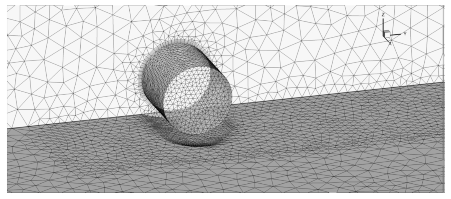
2.3. Adaptive Meshing and Sand-Slide Models

The present study adopts triangular mesh in two-dimensional simulations and tetrahedral mesh in three-dimensional simulations. When using the three-dimensional tetrahedral mesh, the bed surface is divided into triangular elements.

The bed elevation change with time leads to the dynamic change of the bottom boundary of the computational domain. Adaptive meshing enables the computational grid to be updated to fit the new boundary. The adaptive meshing strategy adopted in this paper includes two steps. In the first step, the elevation changes at the centers of the boundary elements are transferred to the boundary nodes. Stresses are stored at the interfaces of the computational cells in FLUENT, hence, the bedload sediment transport rates. Similarly, the bed elevation change, $\mathsf{\Delta }{h}_b$, calculated by Equation (17) at each time step, $\mathsf{\Delta }t$, corresponds to the value at the center of the triangular element on the bed, which needs to be transferred to the boundary nodes. This study uses the area-weighted method to interpolate the bed elevation changes.

$${\lambda }_j=\frac{S_j}{{{\displaystyle \sum }}_{j=1}^m{S}_j}$$

(18)

$$\mathsf{\Delta }{h}_b{}_{node}={\displaystyle \sum }_{j=1}^m{\lambda }_j\mathsf{\Delta }{h}_b{}_j$$

(19)

where $m$ is the number of elements surrounding a node; $S_j$ is the area of the element $j;{\lambda }_j$ is the weight for element $j$; $\mathsf{\Delta }{h}_b{}_{node}$ and $\mathsf{\Delta }{h}_b{}_j$ are the elevation changes at the node and at the center of the element, $j$, respectively. In the second step, the internal nodes and elements are updated to adapt to the new bed shape. In this process, we combine the spring smoothing method and the remeshing method. The spring smoothing method assumes that each two neighboring nodes are connected by a fictitious spring, which all together form a spring network. When a boundary grid point incurs an initial displacement as a result of the bed elevation change, this local movement will spread out to its adjacent grid points by means of the elasticity of the springs, which enables a smooth transition of the local mesh. However, using the spring-smoothing method alone may give rise to entanglement when the displacement at the boundary exceeds the element size. Moreover, the quality of the grid may significantly deteriorate by only using the spring-smoothing method. To solve this problem, FLUENT can mark out the grid cells that are distorted too much and then replace them by undertaking a local remeshing. The combination of the spring smoothing and local remeshing methods can ensure the high grid quality during the bed morphological change, which helps improve the accuracy and stability of the computation.

Because of the complicated behavior of the sediment transport and its nonlinear interaction with the flow field, positive feedback often occurs in the bed elevation update, which may then lead to unrealistic bed profiles and numerical instabilities. An anomaly often occurs when the predicted slope of the scour hole exceeds the repose angle of sediment. Different kinds of rectification techniques, such as backfilling and sand-slide models, have been proposed to overcome this difficulty [21,22]. A sand-slide model is employed in this study when the local bed slope exceeds the repose angle of sediment. The coordinates of the corresponding seabed nodes are adjusted so that the local bed slope becomes equal to the angle of repose while the centroid of the grid cell and the direction of the steepest slope of the bed remain unchanged. For any node, $i$, $Z_i^{old}$ is adjusted to $Z_i^{new}$:

$$Z_i^{new}=Z_i^{old}+\left(\frac{\overrightarrow{A} \overrightarrow{C_i}}{\left|\overrightarrow{A}\right|}\sin \alpha -\frac{\overrightarrow{A} \overrightarrow{C_i}}{\left|\overrightarrow{A}\right|}\cos \alpha \tan \Phi \right)$$

(20)

where $C$ is the centroid of a bed triangular element, and $\overrightarrow{C_i}$ represents the vector from the centroid to the unadjusted node, $i$; $A$ is the direction vector of the fastest bed elevation change before the adjustment.

Figure 1 demonstrates a comparison of the local mesh before and after introducing the sand-slide model in a typical example of scour beneath a sphere. There exist some unreasonably sharp bed irregularities without using the sand-slide model, which may lead to instabilities in the ensuing computations. After applying the aforementioned sand-slide model, the bed shape becomes smoother and more realistic.

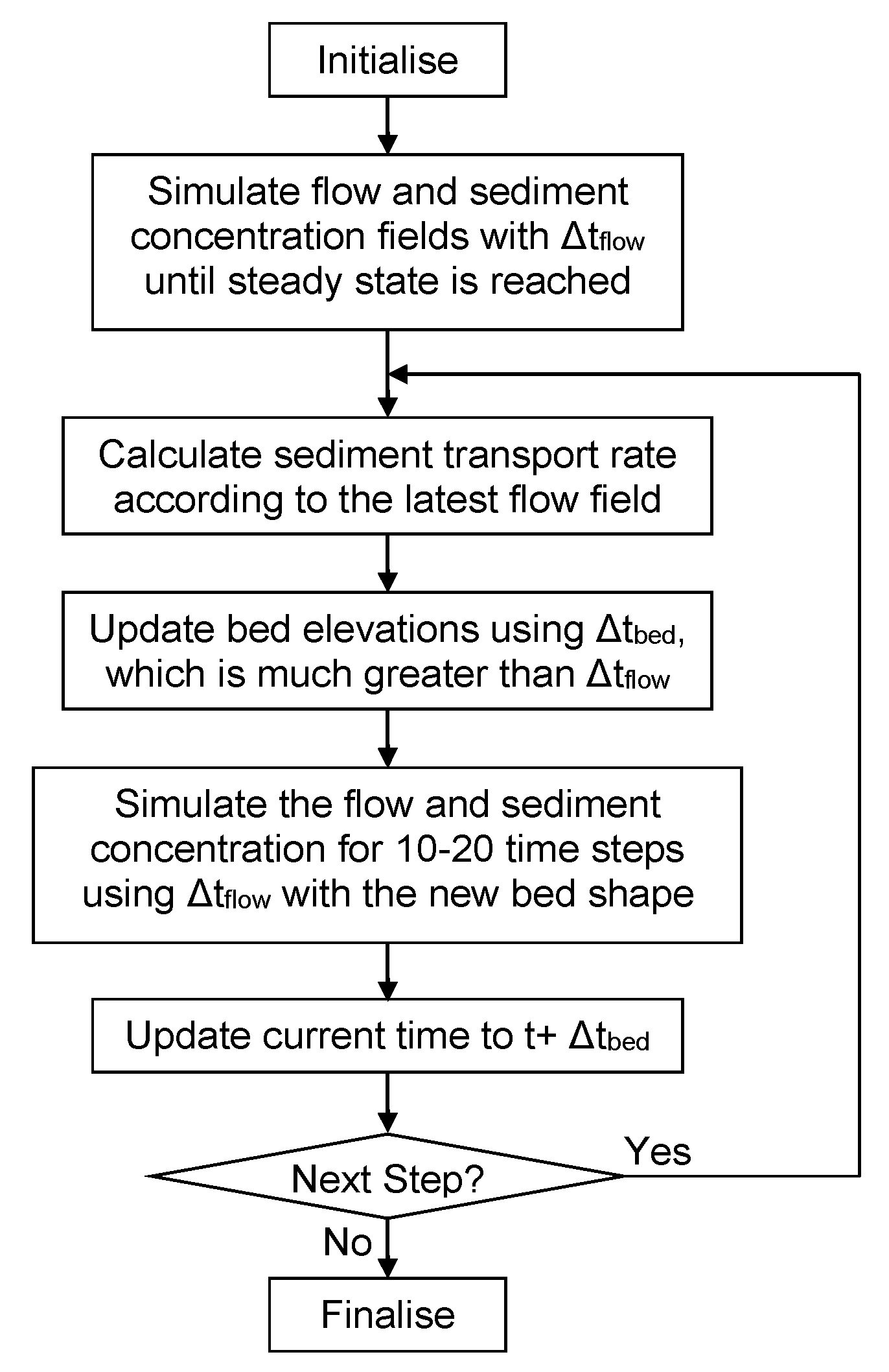
2.4. Numerical Method and Computational Procedure

The software, FLUENT, uses the finite volume method to solve the governing equations, with the computational domain divided into non-overlapping control volumes. The second-order upwind scheme is chosen to approximate spatial derivatives, while the first-order implicit scheme is chosen to approximate temporal derivatives. Within a grid cell, the unknown quantities are assumed to vary linearly, and the spatial derivative and gradient are calculated based on the least-square method. The coupling of pressure and velocity is achieved with the SIMPLEC (semi-implicit method for pressure-linked equations consistent) algorithm, which is one of the SIMPLE’s improved algorithms proposed by Van Doormal and Raithby [23].

The UDFs are a set of functions provided to the user, which serve as the interference to the standard computational procedures in FLUENT. In this study, the UDFs are used to construct the sediment transport and scour models. In calculating the sediment transport load, the UDFs use the F_STORAGE_R_N3V (f, t, SV_WALL_SHEAR) function to extract the bed shear stress information acquired by the flow solver. After solving the bed deformation equation, the bed elevation changes are obtained, based on which the nodes on the bed are moved using the macro, DEFINE_GRID_MOTION. Subsequently, the aforementioned mesh adaptation and sand-slide models are applied to update the mesh.

At the inlet of the domain, the flow is assumed to be fully developed and hydraulically smooth:

$$u\left(z\right)= \min \left\{u_{*}/\kappa \ln \left(z/z_0\right),u_{\infty }\right\}$$

(21)

where the friction velocity is $u_{*}=\kappa u_0/ \ln \left(\delta /z_0\right)$; $\delta$ is the boundary layer thickness; $z_0=2.5d$/30 is the bottom roughness length; $\kappa =0.42$ is the von Karman constant; $u_{\infty }$ is the free stream velocity. The turbulence kinetic energy, turbulence length scale, and turbulence dissipation rate at the inlet are:

$$k\left(z\right)= \max \left\{C_{\mu }^{-1/2} {\left(1-\frac{z}{\delta }\right)}^2{u}_{*}^2,0.0005u_{\infty }^2\right\}$$

(22)

$$l\left(z\right)= \min \left\{\frac{\kappa z}{1+1.5z/\delta },C_{\mu }\delta \right\}$$

(23)

$$\epsilon \left(z\right)=\frac{C_{\mu }^{3/4}\kappa {\left(z\right)}^{3/2}}{l\left(z\right)}$$

(24)

The no-slip wall condition is specified on the solid surfaces inside the domain, including the sand bed and the pipe surface. The outlet flow condition is set at the downstream boundary, and the rigid lid condition is assumed at the top of the computational domain.

Due to the different time scales of the flow field and the bed-shape changes, the hydrodynamic model and the morphological model are coupled in a quasi-steady manner. Different time steps, Δt_flow and Δt_bed, are selected in the hydrodynamic and morphological models to reduce the computational cost. The flow field is assumed to be steady between every two consecutive updates of the bed profile. The computational procedure is shown in Figure 2.

3. Model Verifications

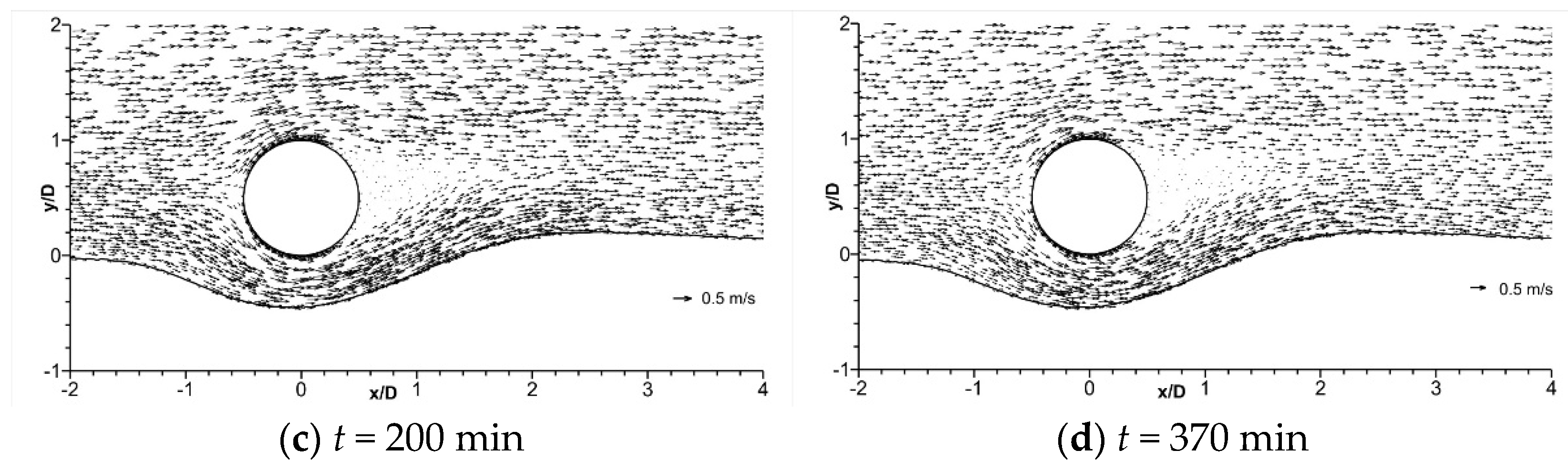
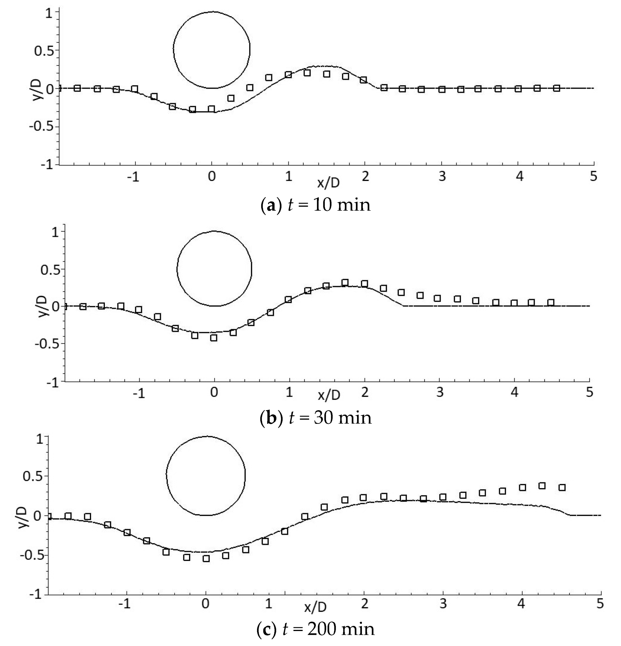
3.1. Vertical Two-Dimensional Scour around an Infinitely Long Pipe

The computation is conducted in a vertical two-dimensional domain of $20D$ in width and 3.$5D$ in height. The pipe is located 8D downstream from the inlet and 12D upstream of the outlet. The pipe sits on the bed, with its bottom at the same level as that of the initial bed. The pipe has a diameter of 100 mm. The diameter of the sediment grain, $d$, is 0.36 mm. The sediment density is 2650 $\mathrm{kg}/{\mathrm{m}}^3$. The repose angle, $\Phi$, is $30°$. The freestream current velocity, $U_{\infty }$, is 0.4 m/s. As a result, the Reynolds number, Re, based on the pipe diameter and the incoming flow velocity, is 40,000 according to Equation (25):

$$Re=\frac{U_{\infty }D}{v}$$

(25)

where $v$ is the kinematic viscosity coefficient of water. The undisturbed Shields parameter, ${\theta }_{\infty },$ can be calculated to be 0.048 by assuming a logarithmic velocity distribution above bed:

$${\theta }_{\infty }=\frac{u_{*\infty }^2}{g\left(s-1\right)d}$$

(26)

where $u_{*\infty }$ is the friction velocity sufficiently upstream of the pipe. The sediment incipient condition can be estimated to be ${\theta }_{cr}$ = 0.034, which is slightly smaller than the undisturbed Shields parameter, indicating a live-bed scour scenario and the dominance of bedload in sediment transport. The depth of the initial scour hole is set to be 0.1D, which is much smaller than the equilibrium scour depth.

When using the local mesh reconstruction algorithm in FLUENT to fit the updated bed boundary, the height of the near-bed grid cells is roughly equal to 0.19 mm, giving the value of the nondimensional distance to the wall, $y^{+}$, of around 5.0. The grid resolution near the bed and pipeline is finer than elsewhere, in order to capture the steep velocity gradient and flow separation. The total number of grid cells is 51,083. Before allowing the bed elevations to change, the calculation is first carried out for a while to obtain a rational flow field corresponding to the initially fixed boundaries.

Figure 3 shows the snapshots of the flow field and bed positions near the pipe at different stages of the scour: from the early rapid-development stage to the final steady-equilibrium stage. For clear visualization, only a third of the velocity vectors are plotted. As shown in the figure, the water flow velocity through the small scour hole is around 0.55 m/s, which is larger than the freestream velocity at the inlet. When t = 10 min, a sand hill with a height of 0.3D appears behind the pipeline. Downstream of the pipe, the flow has a large upward component due to the presence of the sand hill. The steady flow circulation in the wake is restrained and also pushed upwards by the upslope of the scour hole. No vortex shedding is formed. Behind the sand hill, a relatively small clockwise vortex is observed due to the sudden expansion of the flow. As the scour develops, the depth of the scour hole increases and the velocity of the flow through the hole decreases. The length of the scour hole increases faster than the scour depth, so overall the bed slope decreases over time. The wake vortex behind the pipeline becomes gradually horizontal and maintains a length of about 0.5D. The height of the sand hill continually decreases as the sand hill moves downstream. As a result, the vortex behind the sand hill gradually weakens and eventually disappears.

Figure 4 compares the predicted, represented by solid lines, and measured, represented by square symbols, bed profiles at different times. It can be clearly observed that the bed deformation is quick, and the scour hole rapidly grows during $t=10~30$ min, corresponding to the large sediment transport rate around the pipeline. A sand hill is formed as a result of the sand accretion. During this period, the sand hill is seen to move along the flow direction, and the sand accretion height increases. With the increase of time beyond $t=30$ min, the bed deformation slows down. At $t=200$ min, the scour hole continues to deepen, and the depth tends to the maximum value and the sand hill nearly diminishes, although a small backward-facing step at the bed can still be noticed. At $t=370$ min, the scour hole approaches the steady state, and the local bed deformation is negligible. Considering the complexity of the sediment transport and scour phenomena, the simulation results can be regarded to agree well with the experimental results, with only small discrepancies in the scour depth beneath the pipe and the sand hill shape downstream of the pipe.

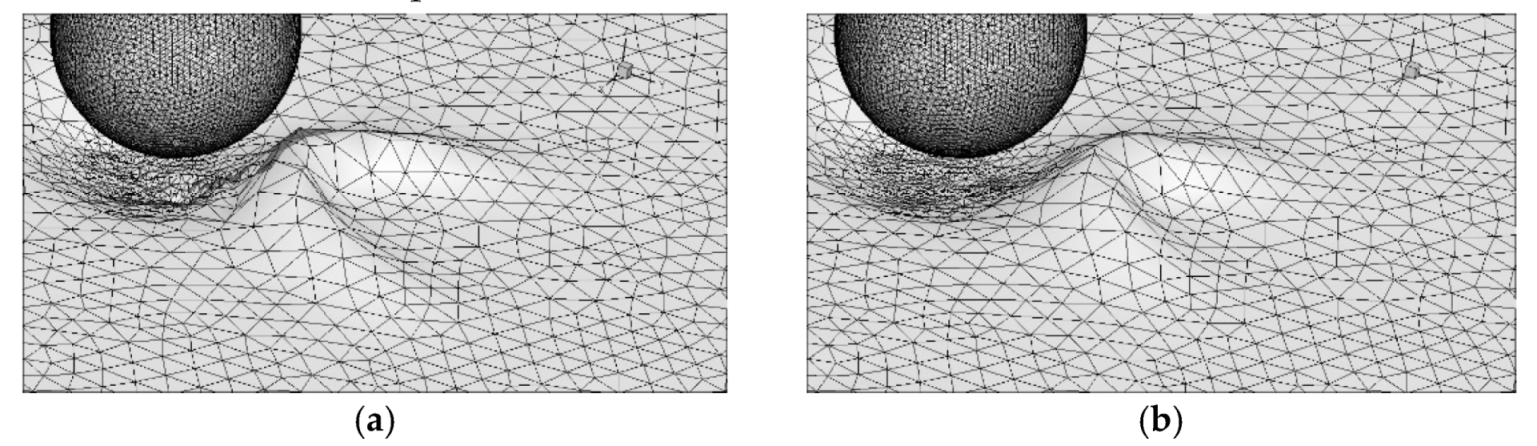
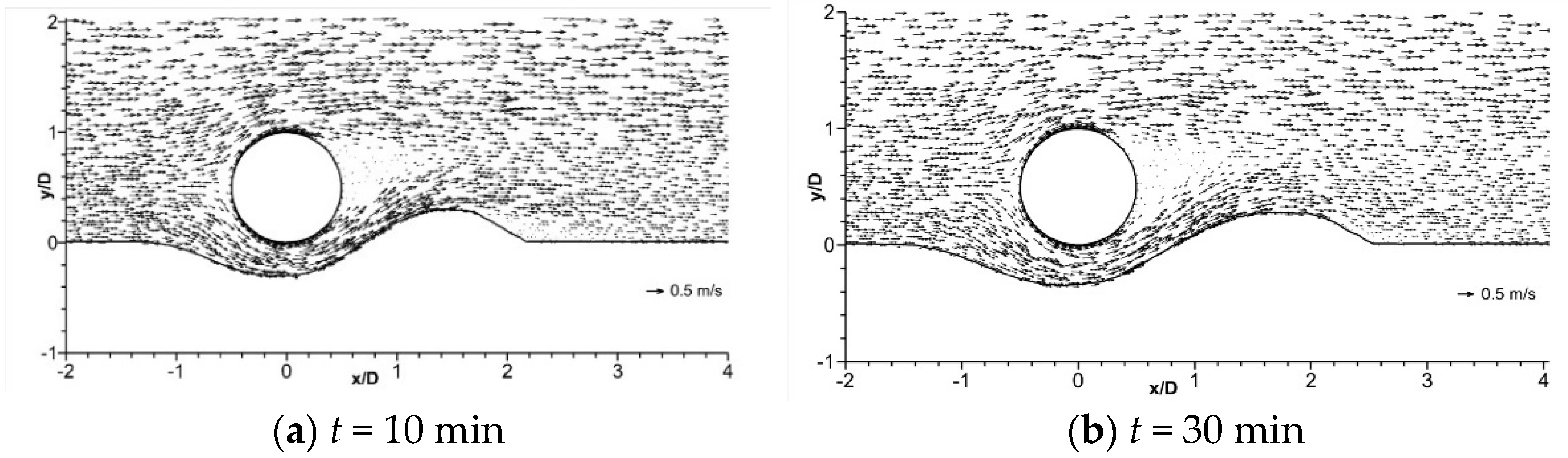
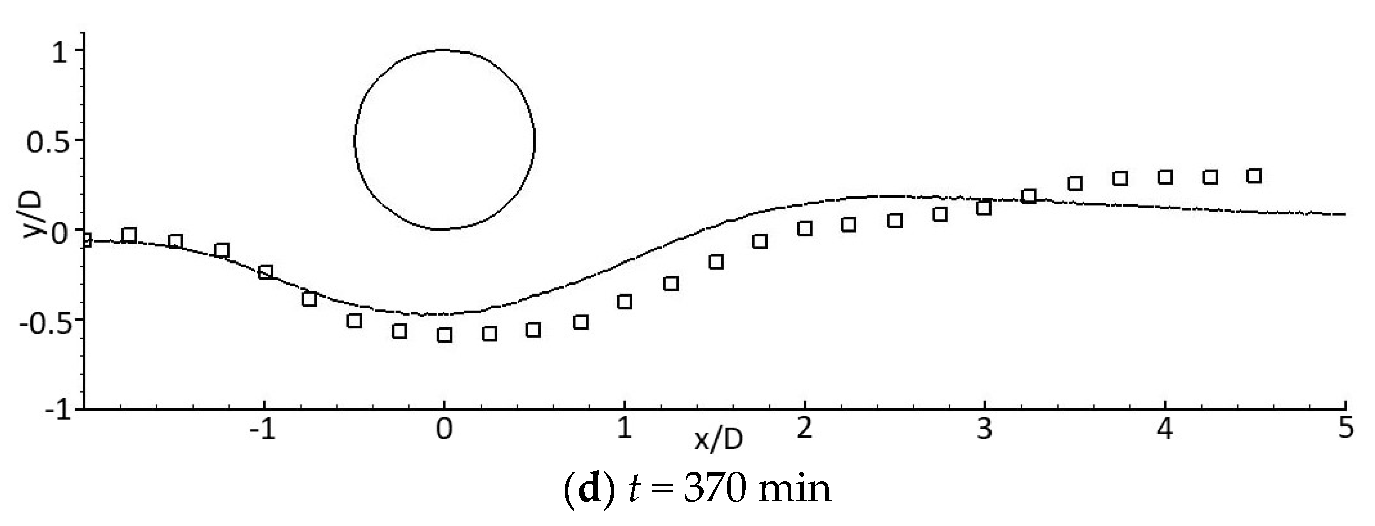
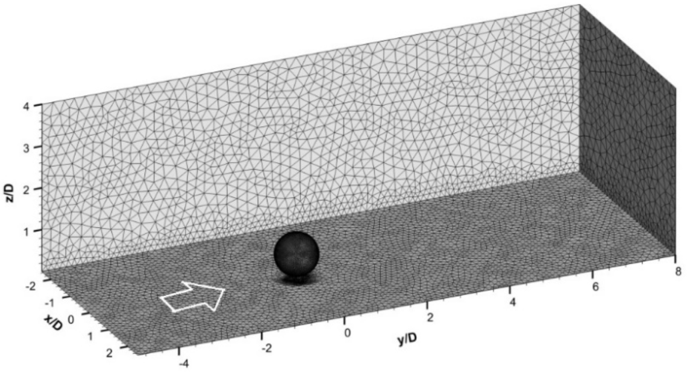
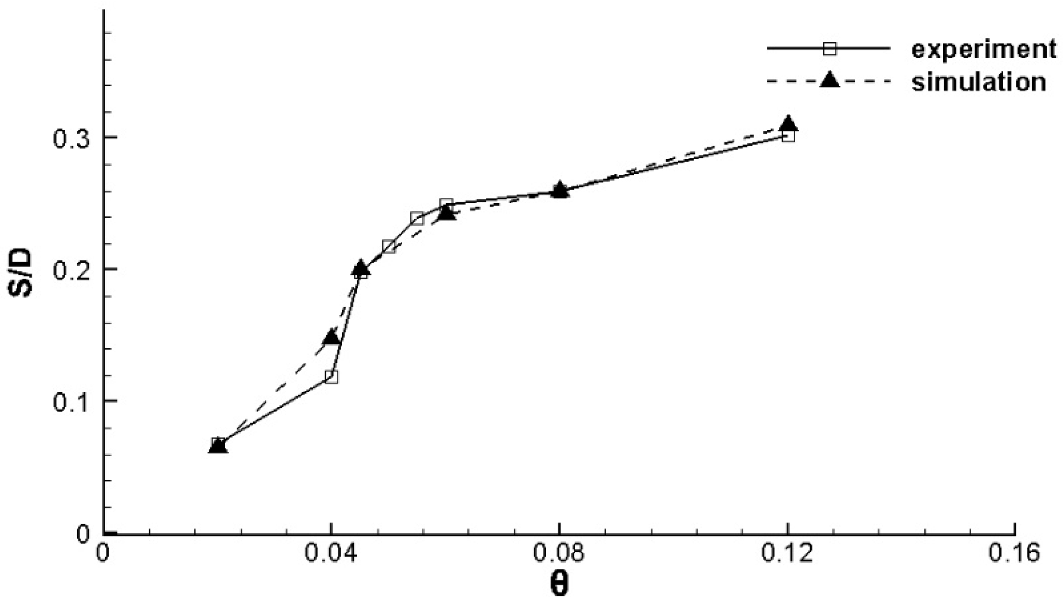
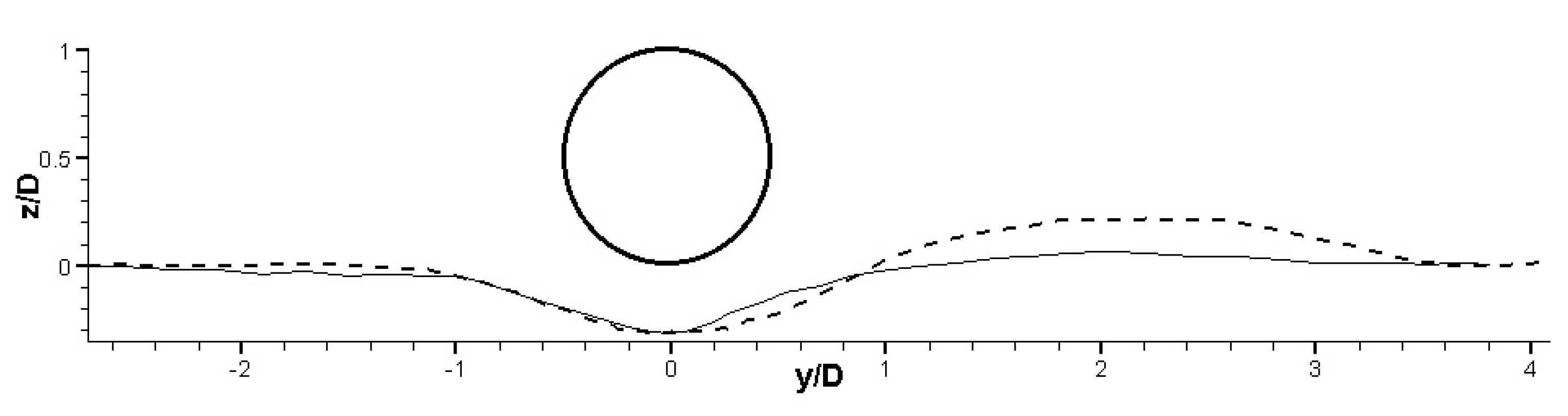
3.2. Three-Dimensional Scour around a Sphere

Figure 5 shows the cuboid domain designed for this three-dimensional problem and computational mesh at the boundary surfaces. The total length of the domain is thirteen times the diameter (13D), with $5D$ upstream and $8D$ downstream of the sphere, which is long enough to reveal the key flow features and scour characteristics around the sphere. The height of the flow domain is $4D$ and the width is $5D$. The total number of grid cells is around 350,000. Dense grid points are allocated around the spherical surface to accurately capture the flow separation and the vortical structures around the sphere, including the horseshoe vortex and arch vortex. Water enters the domain from the left as a fully developed boundary layer flow. The simulation parameters are taken from the experiments reported in Truelsen et al. (2005) [3]. The sphere’s diameter is 60 mm. The diameter of the sediment particles, $d$, is 0.18 mm. The angle of repose, $\Phi$, is $43°$. The bed incipient condition corresponds to ${\theta }_{cr}$=0.05. The incoming Shields parameter is set to different values in different runs: ${\theta }_{\infty }$= 0.020, 0.040, 0.045, 0.060, 0.080, and 0.120, with the corresponding freestream velocities of 0.19, 0.26, 0.38, 0.34, 0.38 and 0.48 m/s, respectively.

A sinusoidally shaped initial scour hole, which is $1.0D$ long and $0.1D$ deep, is initially introduced beneath the pipeline when the undisturbed Shields parameter, ${\theta }_{\infty }$, is more than $0.04$. A relatively deep initial scour hole is introduced to avoid computational difficulties and speed up the scour process to reach the equilibrium stage. However, such a deep initial scour hole may lead to exaggerated scour depth in the early stage, especially in situations with small equilibrium scour depths. If the undisturbed Shields parameter, ${\theta }_{\infty }$, is smaller than $0.04$, then the initial scour hole length and depth are reduced to $0.8D$ and $0.03D$, respectively, considering the relatively shallow equilibrium scour holes in those conditions. The roughness height of the bed is equal to the sediment particle diameter.

As for the case of the pipeline scour at the early stage, sediment is eroded quickly from the small gap between the underneath of the pipe and the bed and a small sand hill is formed as the eroded sediment deposits immediately behind the sphere. An illustration of the scour hole shapes observed in the experiment and predicted in the simulation is given in Figure 6, where the flow is to the right as indicated. Since the information about the lapse of time is missing when taking the photograph of scour, it only allows a qualitive comparison with the simulation result. The computational model successfully captures the general shape of the scour hole beneath the sphere and the sediment deposition behind it.

Figure 7 shows a quantitative comparison between the predicted and measured bed profiles along the centerline of the computational domain when ${\theta }_{\infty }=0.12$. The calculated result agrees precisely with the experimental result in the regions beneath and in front of the sphere. However, the simulated height of the sand hill downstream of the sphere is larger than the measured value, which may be attributed to the neglection of the suspend load in the simulation. When the undisturbed Shields parameter is as large as 0.12, the suspended load has a relatively large influence on the sediment transport in the wake region. The model proposed in this paper ignores the effect of suspended sediment by assuming the bedload dominates sediment transport, which works fine when the Shields parameter is close to the threshold value; thus, it is not surprising that the simulated shape of the sand hill behind the sphere demonstrates some degree of inaccuracy in this case. The bed profiles upstream and downstream of a sphere are more symmetrical than those of a pipeline, which can be explained by the differences between flows around the three-dimensional and two-dimensional structures.

Figure 8 shows the dependence of the equilibrium scour depth on the undisturbed Shields parameter. The simulation results generally agree with the experimental results. As flow intensifies, both the scour hole depth and width increase. In the clear water scour case, the equilibrium scour depth increases rapidly with the increase of the undisturbed Shields parameter. When ${\theta }_{\infty }$ is $0.04$∼$0.045$, the growth rate of the equilibrium scour depth is significant. The increase rate reaches maximum when ${\theta }_{\infty }$ is approximately equal to the critical Shields parameter for the sediment motion, ${\theta }_{cr}$, and at this point the value of the normalized scour depth, $S/D$, exceeds $0.2$. A further increase in the flow speed does not lead to a significant increase in the equilibrium scour depth, as it is the change of the sediment transport rate, rather than the sediment transport rate itself, that decides the scour.

When the value of the undisturbed Shields parameter is $0.04$, the calculated equilibrium scour depth shows an apparent difference from the measured value in the experiment, which may be due to the relatively deep scour hole prescribed at t = 0 in the simulation. However, the comparison is still acceptable considering the large uncertainties in the experiments and empirical formulae used in the computation. In the case of other Shields numbers, ${\theta }_{\infty }=0.045, 0.06, 0.08, 0.12$, the calculated equilibrium scour depths are in excellent agreement with the experimental results, with errors no more than $\pm 0.01D.$ The validity of the adaptive-meshing and time-marching methods stated in Section 2, as well as the correctness of the UDFs, can, thus, be confirmed.

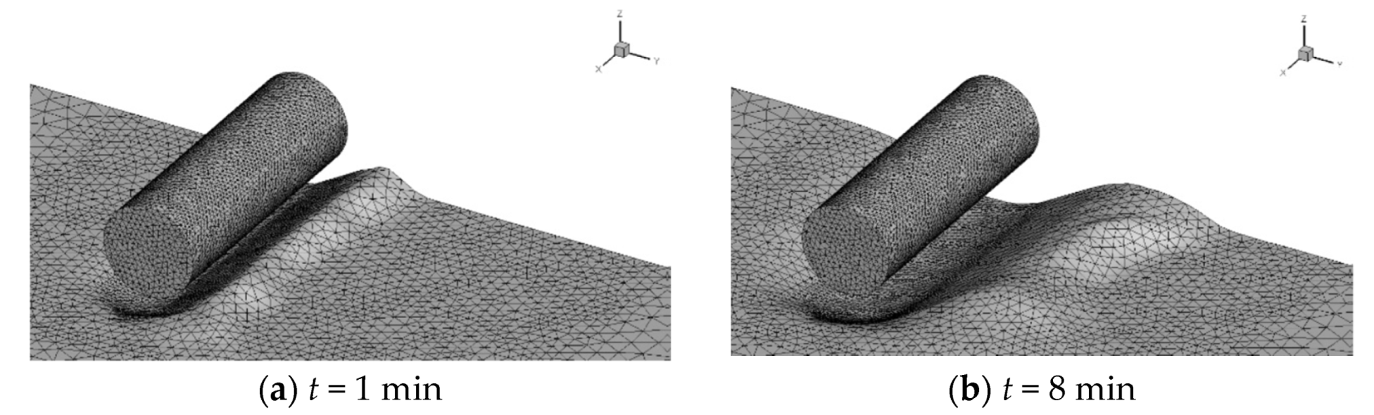
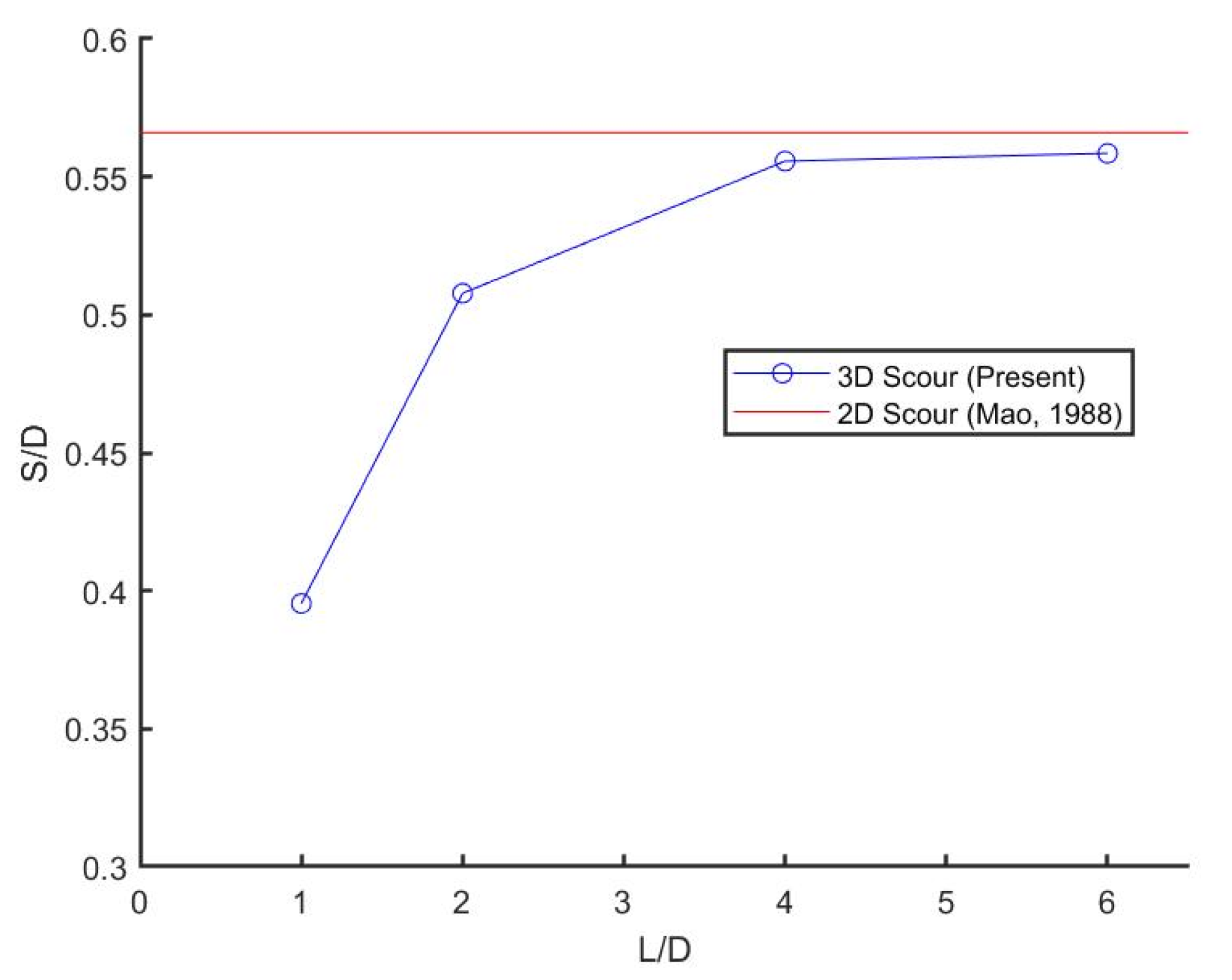
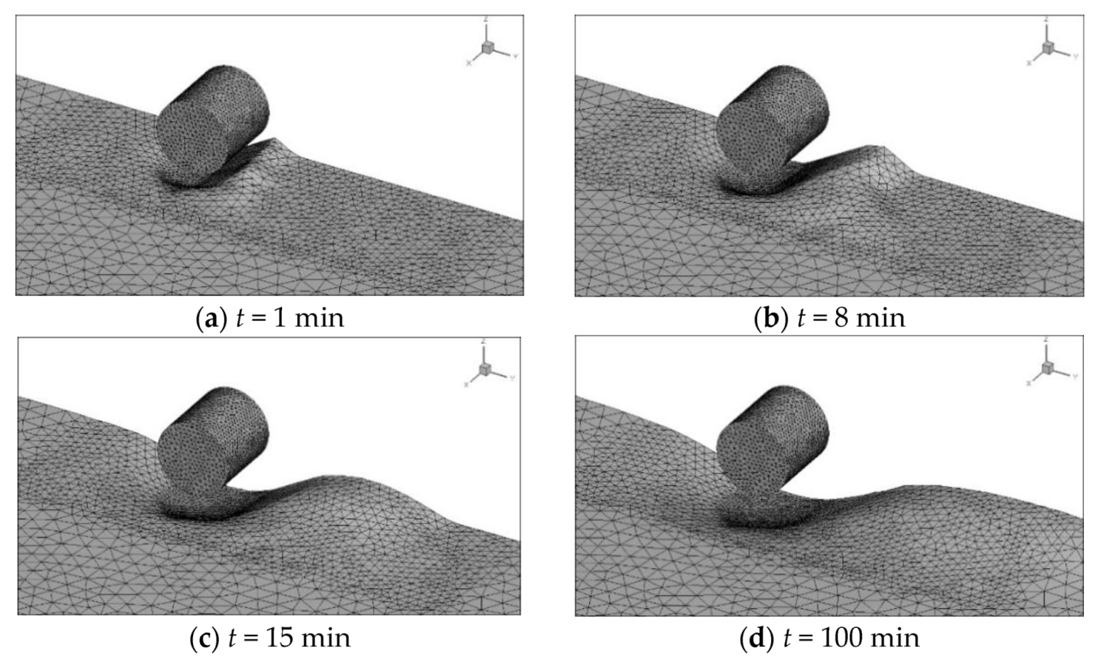
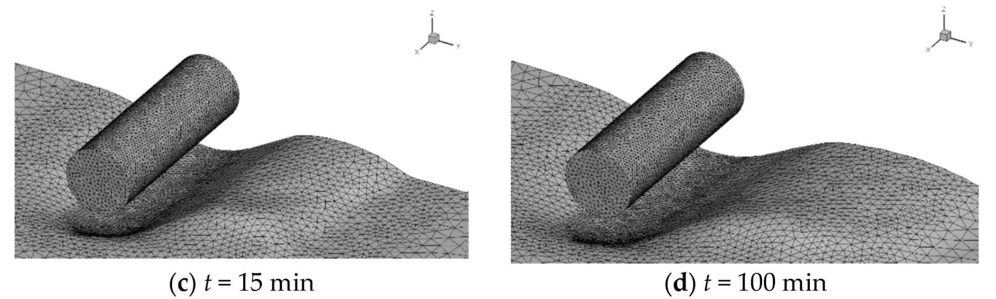
4. Scour around Pipes of Finite Lengths

This section focuses on the application of the established model to investigate the scour around pipes of finite lengths. Figure 9 shows the closeup of an example mesh adjacent to the pipe at the beginning of a simulation. The localized refinement of the mesh near the cylindrical and end surfaces of the pipe can be clearly seen. A cuboid-shaped computational domain is created. A fully developed boundary layer flow, with log-law velocity distribution along the positive $z$-axis, enters the computational domain along the positive $y$-axis from the left. A pipeline with a finite length is located inside the domain with its bottom at the same level as the original bed level. The length of the pipe varies from $2D$ to $6D$. The flow around the pipe is symmetric about the middle $Y-Z$ plane of the pipe, so the computational domain can be halved using the symmetric boundary condition. The inlet boundary is placed $5D$ upstream of the pipe and the outflow boundary is placed $12D$ downstream of the pipe, to enable the sufficient length for the flow and scour to evolve around the pipe. The height of the domain along the $z$-axis is $3.5D$. The width of the domain along the $x$-axis is $5D$, which guarantees an over 2D-wide gap between the end of the pipe and the side boundary to limit the sidewall effects on the flow and scour simulations. The initial manmade scour hole is 0.1D deep and 1D long, and it extends beyond the end of the pipe by 0.5D, as shown in Figure 9. The total number of grid cells ranges from 320,000 to 420,000, depending on the length of the pipe.

Similar computational conditions to Mao’s experiments [2] are applied, with d = 0.36 mm, $\Phi =43°$, ${\theta }_{cr}$= 0.034, ${\theta }_{\infty }=0.048$, and $U_{\infty }=0.42$ m/s. Examples of the scour development around pipes with L = 2D and L = 6D are shown in Figure 10 and Figure 11, which illustrate the bed deformation from the early stage of scour to the equilibrium stage.

From Figure 10 and Figure 11 and simulations performed on the pipelines of other lengths, multiple aspects of the scour hole development can be seen. At the beginning of the scour, the scour depth beneath the pipe increases rapidly. The sand hill behind the pipe is formed as a result of the sediment erosion beneath the pipe and the subsequent deposition. The sand hill is generally higher and migrates downstream faster near the symmetric $y-z$ plane, as compared to the sand hill near the end of the pipe. An exception is observed around a short pipe at the early stage, as evidenced in Figure 10a,b, where the most significant sand hill is seen to appear near the pipe end. Later, however, this portion of the sand hill is slowly washed away by the end vortex, and the bed slope in this region becomes mild. As seen in Figure 10c,d, its height later becomes lower than that near the $y-z$ symmetric plane. When the pipe length is long, the sand hill near the symmetric plane has a similar height to that near the pipe end. The general height of the sand hill varies slightly with the length of the pipe and remains at about $0.25D$ for the two cases presented in these figures.

As the length of the pipe increases, the rate of the scour hole development increases, including the scour hole depth and width. In addition, the sand hill migrates more rapidly downstream of the pipe as the pipe length increases. When the length of the pipe is $2D$, the scour and the flow are strongly three-dimensional around the pipe, leading to the variation of the scour hole shape along the span direction. For a longer pipe, the scour depth and width are relatively unchanged along the centerline of the pipe except near the pipe end, indicating largely vertical two-dimensional characteristics in the middle sections of the pipe.

Figure 12 shows the trend of equilibrium scour depth versus the pipe length with ${\theta }_{\infty }=0.048$. With the increase of the pipe length, the equilibrium scour depth increases, and the effect of the pipe end on flow and scour near the symmetric plane gradually diminishes. When the length of the pipe exceeds 4D, the equilibrium scour depth is close to the two-dimensional results, as reported in Mao (1988) [2], and the scour depth then becomes independent of the pipe length.

5. Conclusions

This study establishes a generic three-dimensional computer model for investigating the scour around underwater structures. The predicted scour processes around an infinitely long pipe and around a sphere are found to be in agreement with those observed in laboratory experiments. Numerical experiments are then conducted to examine the influences of the length of the pipe on the scour depth and sandhill development. The entire model has shown encouraging ability for predicting the local seabed evolution around pipelines and spheres.

As the scour hole deepens, the sand hill downstream of the pipe first grows and then gradually decreases in height as it travels downstream. As the length of the pipe increases, the rate of the scour development increases, and the speed of the sand hill migration downstream also increases. The maximum height of the sand hill appears first near the pipe end for short pipes, while the height of the sand hill is almost constant from the middle symmetric plane to the pipe end when the pipe is long. This can be explained by the flow field characteristics, especially the structure of the wake and end vortices. It has been found that the maximum scour depth increases with the pipeline length until the pipeline length exceeds four times the pipeline diameter. The variation of the local scour width along the spanwise direction is more apparent when the pipe length is smaller. The bed slope is generally milder near the pipe end than that near the middle symmetric plane. It should be noted that these conclusions are obtained from limited parametric studies. More simulations are needed to confirm these findings, especially using the parameters in the prototype conditions.

Using UDFs, this paper introduces a quick way of building a versatile scour model based on a commercial flow solver, FLUENT. A drawback of this strategy is the relatively high computational cost, as the computations of sediment transport and bed deformation and the updates of the computational boundary and mesh are achieved through external interventions to the existing solution procedure of the flow field, rather than seamlessly integrating different submodels at the original source code level.

References

1. Herbich, J.B. Scour around pipelines, piles, and seawalls. In Handbook of Coastal and Ocean Engineering; Gulf Publishing Company: Houston, TX, USA, 1984. [Google Scholar]
2. Mao, Y. The Interaction between a Pipeline and an Erodible Bed; Technical University of Denmark: Lyngby, Denmark, 1987. [Google Scholar]
3. Truelsen, C.; Sumer, B.M.; Fredsoe, J. Scour Around Spherical Bodies and Self-Burial. J. Waterw. Port Coast. Ocean. Eng. 2005, 131, 1–13. [Google Scholar] [CrossRef]
4. Gao, F.P.; Yang, B.; Wu, Y.X.; Yan, S.M. Steady current induced seabed scour around a vibrating pipeline. Appl. Ocean Res. 2006, 28, 291–298. [Google Scholar] [CrossRef] [Green Version]
5. Sumer, B.M.; Jensen, H.R.; Mao, Y.; Fredsoe, J. Effect of lee-wake on scour below pipelines in current. J. Waterw. Port Coast. Ocean Eng. 1988, 114, 599–614. [Google Scholar] [CrossRef]
6. Li, F.; Cheng, L. A numerical model for local scour under offshore pipelines. J. Hydraul. Eng. 1999, 125, 400–406. [Google Scholar] [CrossRef]
7. Chiew, Y.M. Mechanics of local scour around submarine pipelines. J. Hydraul. Eng. 1990, 116, 515–529. [Google Scholar] [CrossRef]
8. Brørs, B. Numerical Modeling of Flow and Scour at Pipelines. J. Hydraul. Eng. 1999, 125, 511–523. [Google Scholar] [CrossRef]
9. Shamloo, H.; Rajaratnam, N.; Katopodis, C. Hydraulics of simple habitat structures. J. Hydraul. Res. 2001, 39, 351–366. [Google Scholar] [CrossRef]
10. Sumer, B.M.; Fredsøe, J. The Mechanics of Scour in the Marine Environment; World Scientific: Singapore, 2002. [Google Scholar]
11. Liang, D.; Cheng, L.; Li, F. Numerical modeling of scour below a pipeline in currents. Part II: Scour simulation. Coast. Eng. 2005, 52, 43–62. [Google Scholar] [CrossRef]
12. Liang, D.; Cheng, L. A numerical model for wave-induced scour below a submarine pipeline. J. Waterw. Port Coast. Ocean Eng. 2005, 131, 193–202. [Google Scholar] [CrossRef]
13. Liang, D.; Li, T.; Xiao, Y. Simulation of scour around a vibrating pipe in steady currents. J. Hydraul. Eng. 2015, 11, 04015049. [Google Scholar] [CrossRef]
14. Yang, B.; Gao, F.; Wu, Y. Numerical Study of the Occurrence of Pipeline Spanning under the Influence of Steady Current. Ship Build. China 2005, 46, 221–226. [Google Scholar]
15. Yang, B.; Gao, F.; Wu, Y. Experimental Study on vortex-induced Vibrations of a Pipeline near a Plane Boundary in Steady Flow. China Offshore Oil Gas 2008, 18, 52–57. [Google Scholar]
16. Hatton, K.A.; Foster, D.L.; Traykovski, P.A.; Smith, H.D. Numerical Simulations of the Flow and Sediment Transport Regimes Surrounding a Short Cylinder. IEEE J. Ocean. Eng. 2007, 32, 249–259. [Google Scholar] [CrossRef] [Green Version]
17. Zhang, Z.; Shi, B.; Fan, F.F.; Ruan, X.J. Two-dimensional numerical simulation of local scour of horizontal cylinder near sand bed. Chin. J. Comput. Mech. 2012, 15, 759–764. [Google Scholar]
18. Van Rijn, L.C.V. Sediment Transport, Part I: Bed Load Transport. J. Hydraul. Eng. 1984, 110, 1431–1456. [Google Scholar] [CrossRef] [Green Version]
19. Allen, J.R.L. Simple models for the shape and symmetry of tidal sand waves: (1) Statically stable equilibrium forms. Mar. Geol. 1982, 48, 31–49. [Google Scholar] [CrossRef]
20. Soulsby, R.; Whitehouse, R. Threshold of sediment motion in coastal environments. Proc. Pac. Coasts Ports 1997, 12, 149–154. [Google Scholar]
21. Jensen, J.H.; Fredsøe, J. Oblique Flow over Dredged Channels. II: Sediment Transport and Morphology. J. Hydraul. Eng. 1999, 125, 1190–1198. [Google Scholar] [CrossRef]
22. Roulund, A. Three-Dimensional Numerical Modeling of Flow around a Bottom-Mounted Pile and Its Application to Scour; Technical University of Denmark: Lyngby, Denmark, 2000. [Google Scholar]
23. Van Doormaal, J.P.; Raithby, G.D. Enhancements of the simple method for predicting incompressible fluid flows. Numer. Heat Transf. 1984, 7, 147–163. [Google Scholar]
Figure 1. Illustration of the scour beneath a sphere with and without sand-slide model. (a) Without sand-slide model. (b) With sand-slide model.
Jmse 10 00106 g001
Figure 2. Flow chart of the time marching procedure.
Jmse 10 00106 g002
Figure 3. Snapshots of the flow field and bed profile around an infinitely long pipe.
Jmse 10 00106 g003aJmse 10 00106 g003b
Figure 4. Comparisons of the computational and experimental scour profiles.
Jmse 10 00106 g004aJmse 10 00106 g004b
Figure 5. Computational domain and boundary mesh for sphere-scour simulation.
Jmse 10 00106 g005
Figure 6. Illustration of the scour shapes in the experiment and simulation, θ = 0.05.
Jmse 10 00106 g006
Figure 7. Predicted (dashed line) and measured (solid line) bed profiles beneath sphere, θ = 0.12 .
Jmse 10 00106 g007
Figure 8. Dependence of the equilibrium scour depth on incoming Shields parameter.
Jmse 10 00106 g008
Figure 9. Closeup of the computational mesh around a short pipe.
Jmse 10 00106 g009
Figure 10. Development of the bed shape for L = 2D.
Jmse 10 00106 g010
Figure 11. Development of the bed shape for L = 6D.
Jmse 10 00106 g011aJmse 10 00106 g011b
Figure 12. Dependence of the maximum scour depth on pipe length, with the horizontal line indicating the scour depth below an infinitely long pipe.
Jmse 10 00106 g012
Publisher’s Note: MDPI stays neutral with regard to jurisdictional claims in published maps and institutional affiliations.