Article

A Method for Measuring Hydrodynamic Force Coefficients Applied to an Articulated Concrete Mattress

1
Department of Civil Environmental and Mining Engineering, The University of Western Australia, Perth, WA 6009, Australia
2
International Joint Laboratory on Offshore Oil & Gas Engineering, Dalian University of Technology, Dalian 116024, China
3
Ocean Graduate School, The University of Western Australia, Perth, WA 6009, Australia
*
Authors to whom correspondence should be addressed.
J. Mar. Sci. Eng. 2022, 10(2), 144; https://doi.org/10.3390/jmse10020144
Submission received: 10 December 2021 / Revised: 20 December 2021 / Accepted: 21 December 2021 / Published: 21 January 2022
(This article belongs to the Special Issue Instability and Failure of Subsea Structures)

Abstract

:
A physical model testing method to determine the hydrodynamic force coefficients of an object is proposed and applied to an articulated concrete mattress placed on a flat surface under steady current condition. The test setup, which comprises of a pulley system that is able to pull the concrete mattress in either direction relative to the flow (e.g., with the flow direction or against the flow direction) and one load cell to measure the force required to pull the mattress, is simple and straightforward. Writing the equations of load balance for two different pulling directions allows the force coefficients to be deduced. The novelty and advantages of the method are that it completely removes the difficulties associated with measuring forces on individual concrete blocks and isolating the mattresses from contacting the solid surface, which were common in conventional test methods for measuring hydrodynamic forces on structures founded on a solid surface. A series of flume tests have been conducted to demonstrate the validity of the proposed method. It is expected that the proposed testing method is applicable to a wide range of structures, bed surfaces and flow conditions.

1. Introduction

Concrete has been the most widely used building material in modern society with justified sustainability [1,2,3]. In this work, we focus on a special type of concrete structure, articulated concrete mattresses (ACMs), which are formed by connected concrete blocks through fabric ropes. AMCs are often used for the purpose of scour protections in various engineering applications. The ropes that connect the concrete blocks ensure a flexible network of blocks which allows the ACM to adjust its geometry to fit over structures and conform to undulations in the river/seabed (e.g., due to scour). The ACM was initially designed and used in the nineteenth century to protect river banks from flood erosion [4]. ACMs have also been used routinely in offshore engineering for scour protection and secondary stabilization measures [5,6,7]. For each of these different applications it is important that the mattress is designed to maintain its hydrodynamic stability under design conditions, which requires knowledge of hydrodynamic forces acting on the mattress.
The hydrodynamic stability of an ACM is governed by the shape of its constituent blocks, the dimensions of the ACM, the interaction of the ACM with its supporting foundation, and the environmental flow conditions [8]. Despite the wide engineering application of ACMs, it is surprising that there is no recommended design practice for assessing their stability in terms of these different governing characteristics. Instead, the design of ACMs is normally based on engineering experience or bespoke laboratory model tests. For example, in the engineering guidelines related to scour production using ACMs issued by National Concrete Masonry Association (US) and Federal Highway Administration (US) [9,10], the drag coefficient is simplified as a value of 1.0 for design. A systematic study of ACM hydrodynamic force coefficients is a key requirement for the development of a recommended design practice, but one has yet to be undertaken.
There have been several investigations into the hydrodynamic stability of ACMs. Melville et al. [11], for example, measured the critical Shields parameter required for cable-tied blocks to roll up from its leading edge. This work accounted for the effect of vertical protrusion of the blocks above the surrounding bed when the mattress was placed in a pit. Griggs [12] carried out three-dimensional numerical simulations to investigate the flow field around two lines of an ACM and to calculate the force coefficients for the constituent blocks. Each line contained eight concrete blocks and, because periodic boundary conditions were used on the sides of the computational domain, the simulation corresponded to an ACM with infinite width. Griggs [12] reported the mean drag and lift coefficients for each of the 8 blocks in a line. The first block has a drag coefficient of 1.54 (when normalised using the frontal area of a block) and all the other downstream blocks have drag coefficients between 0.1 and 0.3. The first block shows a positive lift of 0.28 (when normalised using the plan area of a block) and most of the downstream blocks have a negative lift coefficient that is strongly position dependent. McLaren [8] carried out a series of physical tests with full scale ACM models comprising nine blocks in a configuration of three by three. Six flow directions were examined and the force coefficients on the centre and corner block in the front row were measured using a load cell. It was concluded that the front centre block is the most unstable block for edge lift failure (with a drag coefficient of 0.51 and lift coefficient of 0.18 for the 300 series model). McLaren [8] commented that the load cell has to be fully isolated from the base floor and from other neighbouring blocks to avoid contamination of the load. A similar measuring method with load cells was used by Yamamoto [13] and Hayashi [14] to examine the effect of block geometry on the hydrodynamic force coefficients and the models were also isolated from the floor in the experiments.
To sum up the present limitations in ACM design, Godbold et al. [15] commented that ‘… as no dedicated concrete mattress design code exists some conservatism in the results must be accepted’. Even though research has been conducted to investigate the force coefficients on ACMs (as noted above in Griggs 2014 [12] and McLaren 2019 [8]), the comment from Godbold et al. [15] still remains true today because the knowledge on estimating hydrodynamic forces on ACMs is still limited. Measuring forces on each individual block to then work out the total force is time consuming and unnecessary if the purpose of testing is to develop a method for designing the overall stability of the mattress. Numerical simulation of hydrodynamic forces on such a system is prohibitively expensive due to the need of fine mesh resolution around individual blocks.
With sea-level rise becoming a real global challenge in the 21st century, there may be more applications for using ACMs to protect offshore and coastal structures and riverbanks from erosion and local scour issues. Considering the lack of systematic research concerning hydrodynamic loads on ACMs and the challenges associated with measuring hydrodynamic forces on ACMs using load cells and full numerical simulation, we propose a new testing method to measure the hydrodynamic force coefficients for ACMs. The method allows the determination of total force coefficients without measuring forces on individual concrete blocks, which could be extremely challenging when a large number of blocks are used in a mattress. The new method will complement the methods based on load cells and numerical simulations.

2. Load Balance Analysis for an ACM in Steady Current

An ACM placed on a plane floor and subjected to ocean currents or waves (or combined currents and waves) could lose stability via two different failure modes. In the first mode, the front row of the mattress is lifted by the flow and the ACM rolls up to become unstable. This failure mode is normally defined as edge lift failure [11]. In the second mode, the mattress slides away when the drag force exceeds the frictional sliding resistance. This failure mode is defined as sliding failure.
To quantitatively examine both modes, we consider a mattress laid on a flat seabed and subjected to a current directed normal to the front row of the ACM. The number of blocks in the ACM is defined as m × n , where m is the number of blocks along a line (in the flow direction) and n is the number of blocks along a row. The edge lifting mode is triggered when the hydrodynamic lift acting on the first row of blocks exceeds its submerged weight. Therefore, at the instant of failure, we have
F l i f t , 1 = S W , 1
where F l i f t , 1 is the hydrodynamic lift force on the first row of blocks and S W , 1 is the submerged weight of these blocks. Normally the lift force can be expressed in the form of a lift coefficient C L , 1 , defined so that:
F l i f t , 1 = 0.5 ρ L 1 WU cr , 1 2 C L , 1
where ρ is water density, L 1 is the length of the first row (in flow direction, including the gaps between the block), W is the width of first line, U c r , 1 is the critical reference velocity and C L , 1 is the lift coefficient, which is representative of the average lift coefficient for the blocks in the front row of the mattress. The submerged weight of the concrete blocks can be calculated as:
S W = ρ g ( s g 1 ) H e L 1 W
where s g is the specific gravity of the ACM, H e is the equivalent height of a rectangular block with the same volume as the ACM and the same L 1 and W . Please note S W , 1 = S W / n . By combining the above three equations, C L , 1 can be expressed as:
C L , 1 = 2 ( s g 1 ) ( U cr , 1 2 2 g   H e ) 1
Hence, if experiments are conducted for a particular ACM, we only need to measure the critical velocity for edge lifting failure to work out the corresponding C L , 1 .
It should be noted that the edge lifting failure could also be triggered together with an overturning moment resulting from all the forces acting on the first row of blocks (including, hydrodynamic forces, submerged weight, and contact force). This has been discussed by McLaren and Griggs [8,12]. In this situation (1) may still be applicable, but the lift coefficient would now represent the lift force on a block that may be partially rotated at the time of failure. To obtain the resulting moment on a concrete block and its rotation prior to failure, numerical simulation or direct measurement in model tests is required. This is beyond the scope of the present work.
The sliding failure mode happens when the hydrodynamic drag force exceeds the frictional resistance between the ACM and the floor. The load balance in the horizontal direction at the instant sliding starts can be expressed as:
F drag = μ ( S W   F lift )
where F drag is the total hydrodynamic drag force on the ACM, F lift is the total hydrodynamic lift force on the ACM, μ is the friction factor. This equation can be rearranged as:
0.5 ρ H e WU cr 2 C D + μ 0.5 ρ LWU cr 2 C L = μ ( s g 1 ) g ρ H e LW
where C D and C L are the drag and lift coefficients for the whole ACM, Ucr is the critical velocity for sliding failure and L is the total length of the ACM in the flow direction. Equation (6) can be simplified to give:
( C D + μ L H e C L ) = μ ( s g 1 ) ( U cr 2 2 gL ) 1
Hence, if a test is conducted to measure Ucr at the point of sliding, it is possible to deduce the combined value of C D + μ L H e C L but not the two force coefficients C D and C L , separately. To determine these coefficients separately, a different testing method is required.

3. Proposed Testing Method
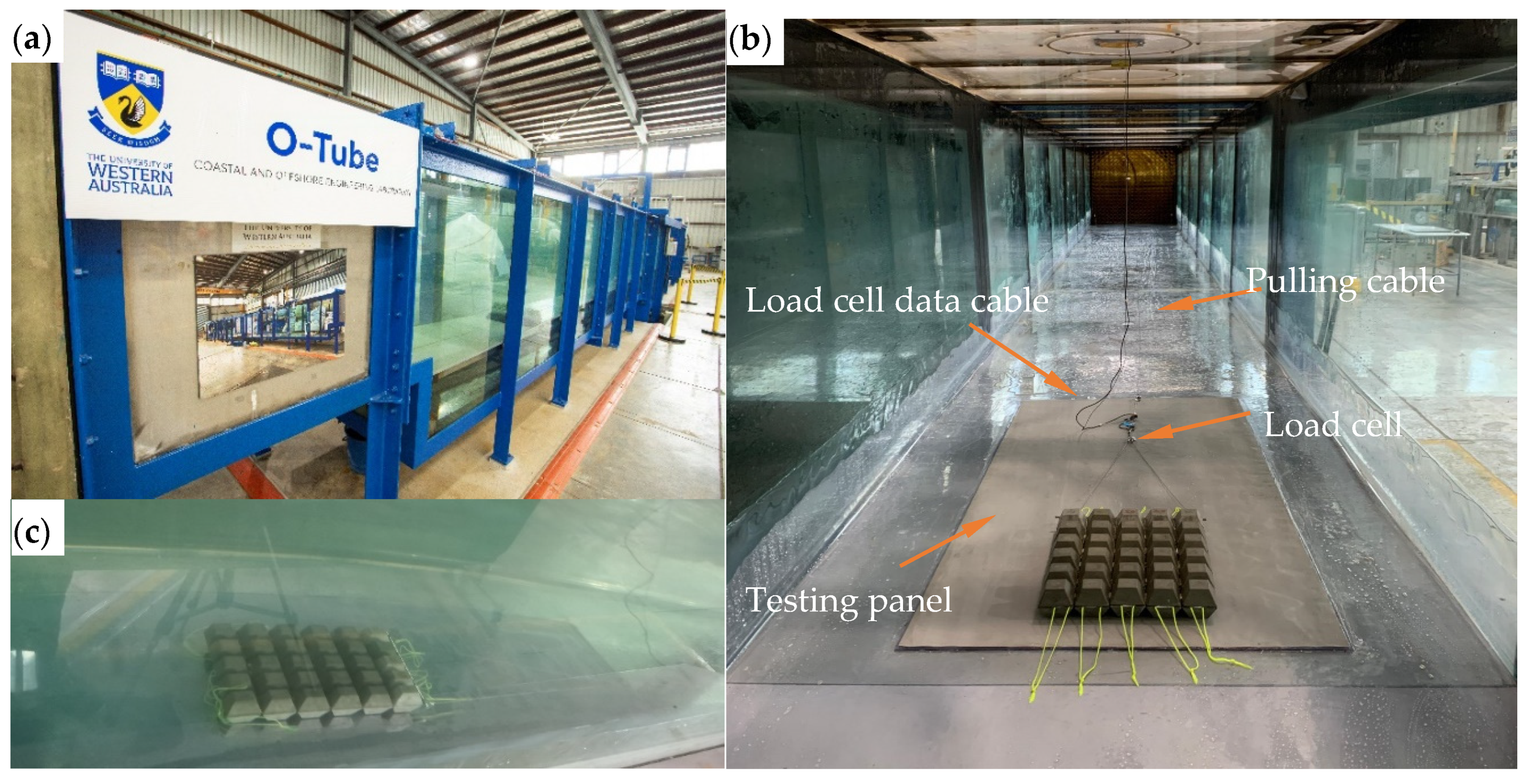
The proposed testing method focuses on the sliding failure mode, for which the analysis is often more straightforward. In practice, the use of a floor with a low friction coefficient can ensure that the sliding failure mode governs, hence allowing application of the testing method proposed below. However, the force coefficients obtained from this method can be applied for ACMs on surfaces with different friction coefficients. The method requires a one-dimensional load cell, an ACM model, a winch, and a water flume. A sketch of the model setup is given in Figure 1. The test procedure includes three main steps as detailed below:
(1) Pull the ACM via the winch at a constant speed in still water. This speed is arbitrary, but must be a sufficiently low value so that the hydrodynamic load experienced while pulling can be ignored (in the present work 0.5 mm/s was used). The pulling load to move the model at this speed is measured using the load cell. The friction factor ( μ ) between the ACM and the floor can then be calculated as the ratio of pulling force to the submerged weight of the ACM.
(2) Generate a steady current with velocity U and pull the ACM so that it slides along the floor in the same direction as the flow at a small, but arbitrary velocity (here a value of 0.5 mm/s has again been adopted). Measure the magnitude of the pulling load ( F p u l l , 1 ) using the load cell.
(3) Reverse the flow direction and pull the ACM against the flow and the pulling speed is kept at a velocity of 0.5 mm/s. Measure the magnitude of the pulling load ( F p u l l , 2 ) using the load cell. This step can be replaced by keeping the flow in the same direction, but pulling the model in the opposite direction. This will be more convenient for flumes without a reversing flow function.
The flow velocity U in Step 2 and Step 3 should be significantly higher than the winch pulling velocity so that the effect of the mattress motion on the hydrodynamic force coefficients can be ignored (i.e., the relative flow velocity is approximately U ).
Because a constant pulling speed is applied to the ACM, no force is associated with its acceleration and the load balance in Step 2 and Step 3 can be written as:
F pull , 1 + F drag = μ ( S W F lift )
F pull , 2 - F drag = μ ( S W F lift )
With the above two linear equations, the two unknown force coefficients can be solved as:
C D = F drag / 0.5 ρ U 2 H e W = ( F pull , 2 F pull , 1 ) / ρ U 2 H e W
C L = F lift / 0.5 ρ U 2 LW = ( 2 S W - ( F pull , 1 + F pull , 2 ) / μ ) / ( ρ U 2 LW )
It is worthwhile to point out here that obtaining unique expressions for the drag and lift coefficient could be achieved with slightly different testing methods to that outlined above. For instance, Step 3 in the procedure can be changed to run at the same flow and winch velocity but to alter the friction coefficient between runs. This would work theoretically but may be less convenient in an experimental campaign than simply changing the flow direction or pulling direction. It would also be possible to extend Step 2 and Step 3 and run similar experiments for multiple different velocity conditions. In this case, the coefficients would be over-determined mathematically, but could be ‘fitted’ in a least square sense.

4. Model Setup

To demonstrate the proposed test method and to compute the hydrodynamic force coefficients, four different ACM models were fabricated. The models have the same configuration as shown in Figure 2, but differ in their specific gravity. For a single block, the middle section measured 0.05 m × 0.05 m, the top surface (and bottom surface) was 0.026 m × 0.026 m and the height was 0.05 m. The ACM configuration was selected to be n × m = 5 × 6, to represent a commonly used arrangement adopted in offshore engineering. For this configuration L = 0.3 m, W = 0.25 m, H = 0.05 m, H e = 0.0338 m and L 1 = 0.05 m at model scale. This model represents a ~1:10 scale model of a full-scale ACM. The s g values of the four ACM models are summarized in Table 1. Model 1 and 2 included lead shot (1.27 mm in diameter) within the cement mix to achieve the high density. Model 3 was made with just cement without aggregate. Model 4 included plastic beads (2 mm in diameter) to reduce the density.
The model tests were conducted in the large O-Tube facility [16] shown in Figure 3a. The O-tube is a recirculating water channel with test section dimensions of 1   m   ×   1   m   ×   15 . 4   m (depth × width × length). The facility has been used to investigate flow-seabed-structure interactions for various applications in offshore engineering. In the present experiments, the solid floor of the O-tube test section was formed by placing a clear PVC sheet on top of a 400 mm sand layer. To provide a stiff base, a panel (with μ = 0.25) was attached to the PVC sheet and used for the majority of the testing program. The test panel covers an area of 0.6 m × 1.2 m and has a thickness of 3 mm.
A picture of the ACM model is given in Figure 3b. A single one-dimensional load cell with 200 N capacity was used to connect the ACM model with the winch, and to measure the pulling load. The pulling cable is a 0.5 mm diameter steel wire. The pulling direction was parallel to the floor of the test section and the pulling cable was brought outside at the end of the test section through a roller. The pulling was controlled by a Clear-Path smart motor (CPM-SDHP-N0561P-ELN) from outside of the test section.
The boundary layer profile above the base floor was measured and it was found that the velocity within 200 mm above the base floor follows a logarithmic profile. The turbulence intensity within the boundary layer reduces from 10% to about 4% with the increase of vertical distance from the base floor. More detailed information about the boundary layer profile can be found in Yang et al. [17].

5. Results

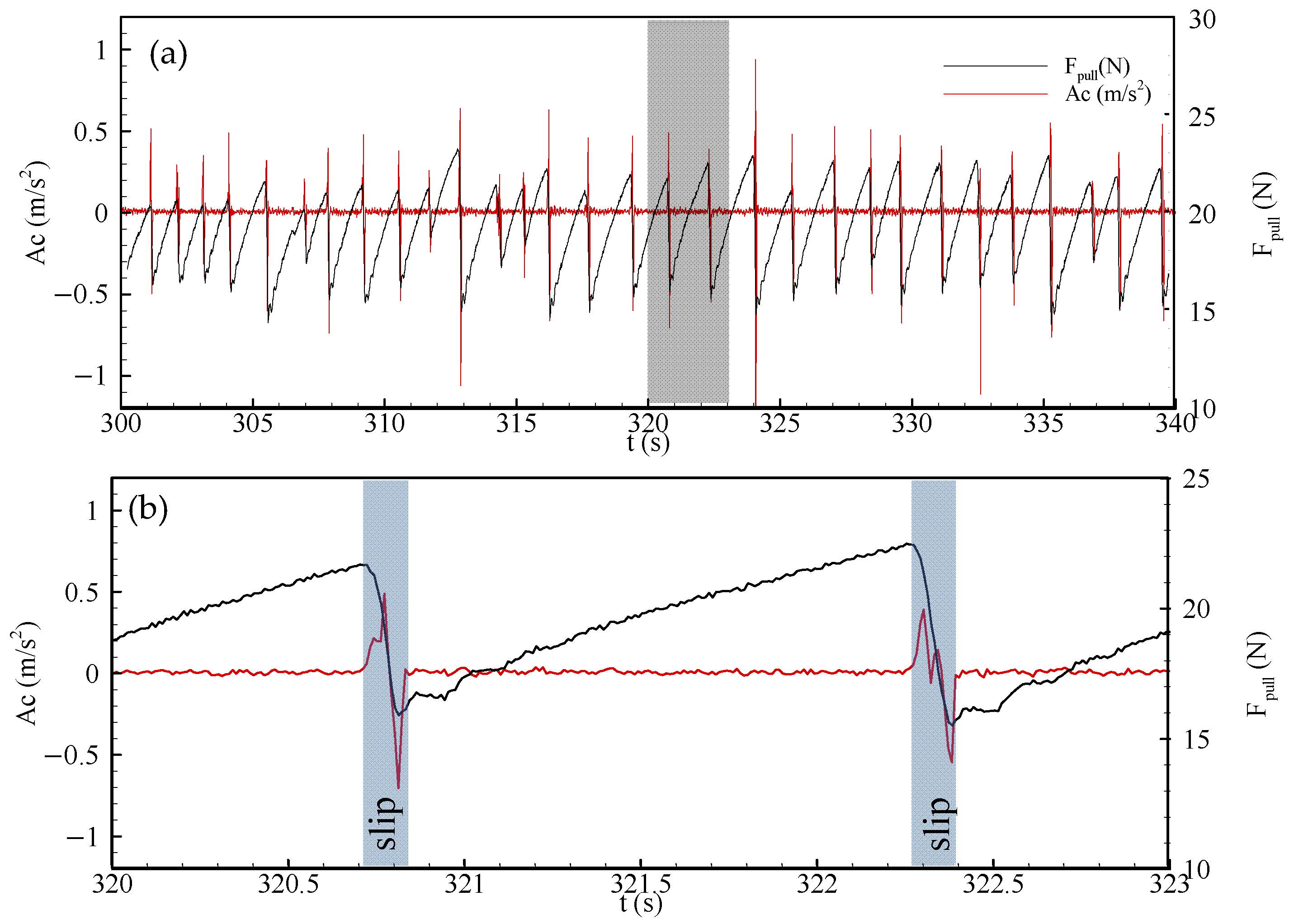
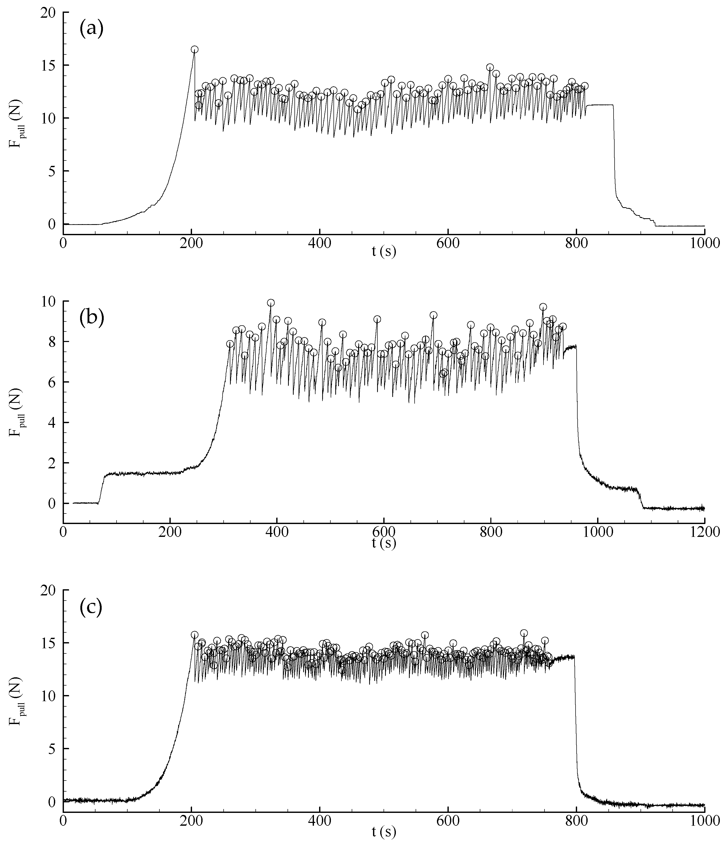
5.1. ACM Sliding Behaviour

As the concrete blocks in the ACM are connected with soft ropes, the ACM is flexible. The sliding behaviour could be different from that of a rigid body sliding on a solid surface. A pulling test was carried out to examine the sliding behaviour of the ACM. The test setup was similar to that shown in Figure 3b. The ACM ( s g = 3.23) was pulled in air by the motor with a pulling velocity of 0.5 mm/s. Besides the pulling load measurement, an accelerometer was attached to the ACM to examine the motion of the ACM.
The test duration was 600 s and the ACM was pulled over 300 mm. Although a constant pulling speed was applied from the motor, the mattress moved with a stick-slip behaviour. The measured data is presented in Figure 4a, where the pulling load ( F p u l l ) shows a saw-tooth shape and the acceleration measurement remains at zero with occasional pulsing features due to the stick-slip behaviour. Instead of a smooth moving process, the stick-slip behaviour is very often seen when a solid object is pulled over a flat surface. Some discussions about the mechanism of the behaviour at the interface have been provided by Byerlee [18] and Thompson and Robbins [19]. A zoom-in view of measurement is given in Figure 4b to examine the key features of the data. It shows that the pulling load was gradually building up while the acceleration (defined as A c ) remains at zero (no ACM movement) for t = 320.0 s~320.70 s. When the pulling load reached a local peak value of 21.6 N, the accelerometer reading shows a sudden zig-zag pulse, which corresponds to one slip of the ACM. A data logging frequency of 100 Hz was required to resolve the pulses in the accelerometer reading. Meanwhile the pulling load experienced a sudden drop to 16.1 N. The peak pulling load of 21.6 N corresponds to the maximum static friction force on the ACM. After A c returned to zero at t = 320.84 s (the ACM stopped moving) and the pulling load gradually built up again until the next step of slip (t = 322.26~322.40 s). The shadow area shown in Figure 4b represents the time when the ACM was moving and for the rest of the time the ACM remained still. By analyzing the whole test data sequence, the ACM remained still over 93.5% of the pulling test. Therefore if we only count the time when the ACM was moving, the averaged moving speed of the ACM can be calculated as U A C M = 0.05   mm / s ÷ ( 1 93.5 % ) = 7.7 mm/s, which is much faster than the pulling speed of the motor. This is the reason why the pulling load shows the saw-teeth behaviour. After each step of the ACM slip, the pulling cable relaxed slightly because the slipping speed was higher than the pulling speed, and this led to the reduction of the pulling load. After the pulling load dropped to a local minimum value, the ACM stopped, and the pulling load gradually built up again.
The important information we extract here is that the peaks of the pulling load represent the maximum static friction between the floor and the ACM. This information is used to determine the hydrodynamic force coefficients in the following section. The accelerometer was only used in this test to understand the stick-slip behaviour and it was removed from the model for the remaining tests.

5.2. Sliding Failure Mode

This section presents results from the three-step test procedure given in Section 2 to work out the force coefficients on the ACM under steady current conditions.
In the first step, the friction factor was determined in still water by pulling the ACM at 0.5 mm/s. The measured pulling force in a typical test case is given in Figure 5a. The logging frequency is 10 Hz, which is sufficient to resolve the variation of the pulling load. In the first 200 s, the tension in the pulling line gradually built up to 16.5 N, at which point the ACM started to move. Following this, the load cell reading suddenly dropped to 9.2 N and then gradually built-up again. In the pulling test shown in Figure 5a, the model moved 300 mm over 600 s with a total of 93 local peaks. Therefore, the mattress moved about 3.2 mm in each slip on average. The peaks associated with a subsequent load drop less than 10% of the averaged load drop are ignored since these peaks were mainly due to electrical noise in the logging system. The peaks of the load cell reading represent the maximum static friction force between the ACM and the floor as demonstrated in the previous section. During the slipping phase, the ACM experiences slight accelerations and then deceleration before the slipping process repeats itself again. This means the forces on the ACM are not in equilibrium during the slipping phase and the load balance equations should not be used during the slipping phase. Therefore, only the information in the static phase should be considered when solving the load balance equations (Equations (8) and (9)). The other consideration is that we focus on the sliding failure and the peak pulling forces in the time history corresponding to the critical conditions before sliding failure happens. Therefore, the peak pulling forces were used to determine the friction factor and to calculate the force coefficients based on Equations (8) and (9). We believe the friction factor determined based on the peak pulling forces represents the true static friction factor. The mean value of the peaks in Figure 5a is 12.7 N. Adopting this result, the maximum static friction factor of the ACM is calculated to be μ   = 0.25. The effect of pulling speed was also tested; pulling at 0.1 mm/s had no obvious effect on μ . Therefore, the pulling velocity of 0.5 mm/s was used for the rest of the testing program.
Corresponding to Step 2 of the test procedure, a flow of 1.0 m/s was generated and the ACM was pulled in the same direction as the flow. The pulling load time history is given in Figure 5b. The reference velocity was measured 1 m upstream of the model and 150 mm above the floor level. The ACM load cell also showed a stick-slip behaviour while it was pulled. The mean value of the peaks is 8.6 N and this is the F pull , 1 value adopted for use in Equation (8).
Finally, in Step 3, the flow was changed to −1.0 m/s so that the ACM was pulled against the flow. The load time history is shown in Figure 5c. The ACM also moved 300 mm over 600 s, but the number of peaks can be seen to have increased to 180, with a step averaged distance of 1.7 mm. This is because when flow is against the movement of the ACM, it tends to resist the ACM movement. The average of the peaks is 14.1 N.
The frequency spectra associated with the pulling forces (shown in Figure 5) are presented in Figure 6 with a frequency f less than 0.5 Hz, beyond which the energy level is very low. An important feature observed from the spectra is that the load fluctuation during the pulling process does not have a dominant frequency. For the results in still water (Figure 6a), the three peaks with relatively high energy are observed in the range of f = 0.1 and 0.15 Hz. Under the condition of U = 1 m/s, the major frequencies shifted to a lower range of f = 0.07 to 0.12 (Figure 6b). When the model was pulled against the flow (U = 1 m/s), the peak frequency moved to a much higher value (f = 0.27 Hz, shown in Figure 6c). This is consistent with the model moving slightly further in each jump when pulled in the direction of the flow (3.2 mm on average compared to 1.7 mm); hence, as the winch velocity was constant, the time between events was slightly longer and the associated frequency was therefore lower. Through this frequency analysis, we also can confirm that the oscillations of the measured loads are not induced by any flow mechanisms, such as vortex shedding from the edges of the blocks, as the oscillations of the measured loads also exist in the still water test, as shown in Figure 5a. This argument is further supported by the frequency spectra shown in Figure 6, where no obvious dominant frequencies exist.
Combining the information in the above three steps, the force coefficients C D and C L can be calculated according to Equations (10) and (11). This procedure was conducted three times and a summary of the test results is given in Table 2. T1 and T2 were conducted with ±1.0 m/s flow velocity and T3 was conducted with ±0.8 m/s. The average force coefficients obtained from these three tests were C D = 0.633 and C L = 0.167 .
These force coefficients have been validated in two ways. Firstly, the values of C D = 0.633 and C L = 0.167 were used to predict the load cell pulling force required at different flow velocities. Two pulling tests were conducted with U = 1.20 m/s and 1.38 m/s (T4 and T5) and the measured F p u l l , 2 are summarized in Table 3. The difference between predicted (from Equation (9)) and measured F p u l l , 2 values are 8.3% and 1.9%, respectively.
In the second group of validation tests, the pulling system was removed and the flow velocity was increased using a constant acceleration of 0.55 mm/s2. This flow acceleration was chosen to be very low so that the induced inertia force on the ACM can be ignored. An example flow velocity time history is given in Figure 7, which was measured from test T6 with s g = 3.23. It can be seen that the flow velocity increases from 1.05 m/s to 1.85 m/s over 1500 s. It was observed that the ACM started to slide on the test panel at 1.8 m/s, which is based on a moving average of the velocity measurement over 20 data points (over 2 s). Therefore 1.8 m/s was defined as the critical flow velocity for sliding failure. Three ACM models with different s g values were tested (T6, T7 and T8). For each ACM model, the sliding tests were conducted five times and the measured critical velocities are summarized in Table 4. It can be seen that Ucr reduces with s g , as expected. The predicted Ucr values using Equation (7) for the three ACM models are also given in Table 4. It is found that the difference between the measured and predicted Ucr values are in the range of 1% to 4%. According to the two groups of validation tests, C D = 0.633 and C L = 0.167 give reasonable predictions of the hydrodynamic behaviour for this ACM.

5.3. Edge Lifting Tests

A group of edge lifting tests were conducted using the ACM with s g = 1.72. The test procedure is identical to that used in tests T6–T8. No external pulling was applied to the ACM and the flow velocity is gradually increased until the model started to move. Because of the low s g value of the ACM model, the model lost stability due to edge lifting failure. Five repeat tests were conducted, and the average critical velocity was found to be 0.96 m/s. This leads to a lift coefficient (based on Equation (4)) of C L , 1 = 0.517. According to this force coefficient, the critical edge lifting velocity will be U c r = 1.53 m/s for the ACM with s g = 2.21 (in Test 8), which is higher than the sliding failure critical velocity (1.38 m/s). This is consistent with sliding failure happening in T8, instead of edge lifting. We also noticed that C L , 1 is about three times larger than the total lift coefficients of the full mattress ( C L ). This is because the downstream blocks tend to have lower lift or even negative lift coefficients as reported by Griggs [12]. The lift coefficient for the front middle block (in a 3 × 3 configuration) is in the range of 0.17 to 0.26 for three different block geometries (McLaren 2019) [8]. This is much lower than the C L , 1 value obtained in present work. This can be attributed to two reasons. Firstly, the ACM layout in McLaren [8] is different from that of the present tests. Secondly, the load cell measurement has to isolate the block from the floor. This means a small gap is hard to avoid between the block and the floor. This gap does not affect the drag force much but will have a significant effect on the lift coefficient. For example, when a cube is lifted up from a floor with a gap of 8% of the edge length, the lift coefficient shows a change from 0.6 to 0.1 [20].

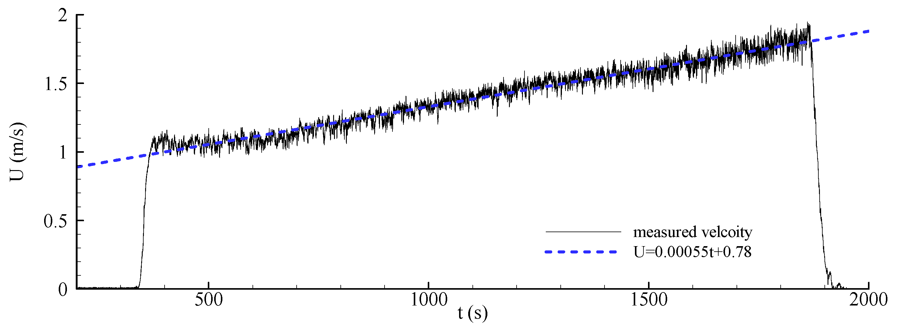
5.4. Reynolds Number Effect

It should be noted that the test method proposed in this paper has its own limitations due to the similarity in Reynolds number between the prototype and model not being enforced. Thus, it is advisable that scaled model tests with this method should be applied to those objects where hydrodynamic forces on them are relatively insensitive to the Reynolds number. An obvious choice of Reynolds number in the present setup is R e = U H / ν , where ν is the kinetic viscosity of the fluid. Generally speaking, hydrodynamic forces on objects with sharp corners, such as square cylinders [21], are insensitive to Re over wide ranges of Re, as locations of flow separation from the structure (such as squares, cubes and ACM) are fixed at the sharp edges on the objects.

6. Conclusions and Recommendations for Further Work

6.1. Conclusions

In this work, a new testing method is proposed to evaluate the hydrodynamic force coefficients acting on an ACM. A series of model tests were conducted at a model scale of 1:10 with an ACM configuration of 5 × 6. The major conclusions are given as below.
(1) A pulling test procedure is proposed. In the procedure, an ACM model was pulled both in the same and the opposite direction to a steady current flow. From measurements of the force required to pull the mattress in both directions, the hydrodynamic drag and lift coefficients can be obtained.
(2) The force coefficients obtained for the ACM were validated by predicting the load cell force and the critical velocity due to sliding under different conditions and comparing these results with experiments. Reasonable agreement was achieved between the measured and predicted values, with a maximum error of 8.3% across five validation tests.
(3) The edge lift failure regime was also tested and the lift coefficient on the front row was obtained. This lift coefficient was larger than that obtained for sliding because the front row of blocks is not shielded.

6.2. Recommendations for Future Work

The results presented in this work are intended to demonstrate the new test method. More tests are needed to examine how the force coefficients are affected by the geometry of the blocks, ACM layout, boundary layer profiles, flow directions and flow conditions besides current (such as waves, combined waves and currents, etc.). A set of experiments covering a realistic parameter space mapped out by these input parameters would provide a solid basis for the development of design guidelines for ACMs. Importantly, the method presented here to measure force coefficients is fast compared to computational methods and experimental methods that need to resolve the force on each block individually, hence it would appear to be ideal for a parametric study of this kind.
On a sandy seabed, local scour will also play an important role in determining the stability of an ACM and any supported structures. Understanding the effects of local scour around ACMs is limited at present and more research is needed. Some flow visualization (through physical model tests or numerical simulations) will be beneficial to understand how ACMs interact with boundary layer flow over a seabed.
Several aspects of the proposed test method could be investigated further, including an assessment of the most ideal friction coefficient to use and the background flow velocities to ensure the most reliable estimates of the force coefficients. Further work could also be undertaken to apply the method in wave or combined wave and current conditions. This work would be valuable because the proposed testing method would be generally appropriate for obtaining force coefficients of rigid structures sitting on a plane floor and submerged in boundary layer flow. Examples include gravity anchors, subsea infrastructure for offshore energy developments and artificial reefs structures; all of which resemble gravity-based structures placed onto a flat seabed.

Author Contributions

Conceptualization and methodology, H.A., S.D. and L.C.; Testing setup: H.A., B.L. and M.K.; testing conduction and data analysis, H.A.; Writing—original draft preparation: H.A., X.H., S.D., L.C., B.L. and M.K.; writing—review and editing, H.A., X.H., S.D., L.C., B.L. and M.K.; All authors have read and agreed to the published version of the manuscript.

Funding

This research received no external funding.

Data Availability Statement

The data presented in this study are available through sending request to [email protected].

Conflicts of Interest

The authors declare no conflict of interest.

References

  1. Scope, C.; Vogel, M.; Guenther, E. Greener, cheaper, or more sustainable: Reviewing sustainability assessments of maintenance strategies of concrete structures. Sustain. Prod. Consum. 2021, 26, 838–858. [Google Scholar] [CrossRef]
  2. Hrabova, K.; Lehner, P.; Ghosh, P.; Konecny, P.; Teply, B. Sustainability Levels in Comparison with Me-chanical Properties and Durability of Pumice High-Performance Concrete. Appl. Sci. 2021, 11, 4964. [Google Scholar] [CrossRef]
  3. Zhang, Z.; Gong, R.; Zhang, H.; He, W. The Sustainability Performance of Reinforced Concrete Structures in Tunnel Lining Induced by Long-Term Coastal Environment. Sustainability 2020, 12, 3946. [Google Scholar] [CrossRef]
  4. Dardeau, E.A., Jr.; Ellis, S.W.; Collins, J.G. The articulated concrete mattress: History and use. Erosion and its control. In Proceedings of the Federal Interagency Sedimentation Conferences, Las Vegas, NV, USA, 18–21 March 1991. [Google Scholar]
  5. Gaeta, M.G.; Lamberti, A.; Galante, F.; Mongiorgi, M. Articulated concrete block mattresses (ACBM) for submarine pipeline protection and stabilization: A physical model study in a wave flume. In Proceedings of the Marine Waste Water Discharges and Coastal Environment + International Exhibition on Materials, Equipment and Services for Coastal Environmental Projects, Dubrovnik, Croatia, 27–31 October 2012. [Google Scholar]
  6. Yamini, O.A.; Kavianpour, M.R.; Mousavi, S.H. Wave run-up and rundown on ACB Mats under granular and geotextile filters’ condition. Mar. Georesources Geotechnol. 2018, 36, 895–906. [Google Scholar] [CrossRef]
  7. Yamini, O.A.; Mousavi, S.H.; Kavianpour, M. Experimental investigation of using geo-textile filter layer in articulated concrete block mattress revetment on coastal embankment. J. Ocean. Eng. Mar. Energy 2019, 5, 119–133. [Google Scholar] [CrossRef]
  8. Mclaren, R.W.G. Investigation of Hydrodynamic Forces on Articulated Concrete Block Mattresses in Fluid Flow from Various Horizontal Directions. Master’s Thesis, University of Tasmania, Churchill Ave, TAS, Australia, March 2019. [Google Scholar]
  9. NCMA (National Concrete Masonry Association). Design Manual for Articulating Concrete Block (ACB) Revetment Sys-Tems; Publication No. TR220A; NCMA (National Concrete Masonry Association): Herndon, VA, USA, 2010. [Google Scholar]
  10. Lagasse, P.F.; Clopper, P.E.; Pagán-Ortiz, J.E.; Zevenbergen, L.W.; Arneson, L.A.; Schall, J.D.; Girard, L.G. Bridge Scour and Stream Instability Countermeasures: Experience, Selection, and Design Guidance: Volume 2 (No. FHWA-NHI-09-112), 3rd ed.; National Highway Institute (US): Arlington, VA, USA, 2009.
  11. Melville, B.; Van Ballegooy, R.; Van Ballegooy, S. Flow-induced failure of cable-tied blocks. J. Hydraul. Eng. 2006, 132, 324–327. [Google Scholar] [CrossRef]
  12. Griggs, R. 3D CFD Investigation of Hydrodynamic Forces on Subsea Articulated Concrete Mattresses. Bachelor’s Thesis, Edith Cowan University, Joondalup, Australia, 2014. [Google Scholar]
  13. Yamamoto, K.; Hayasi, K.; Senkine, M.; Fujita, K.; Tamura, M.; Nisimura, S.; Hamaguchi, K. Measuring method of drag coefficient, lift coefficient and equivalent roughness of re-vetment block. J. Jpn. Soc. Civ. Eng. (Hydraul. Eng.) 2000, 44, 1053–1058. [Google Scholar]
  14. Hayashi, K. Fluid forces and stability for block with seaweed. J. Jpn. Soc. Civ. Eng. Ser. B3 (Ocean. Eng.) 2018, 74, 360. [Google Scholar] [CrossRef] [Green Version]
  15. Godbold, J.; Sackmann, N.; Cheng, L. Stability design for concrete mattresses. In Proceedings of the Twenty-fourth International Ocean and Polar Engineering Conference, Busan, Korea, 15–20 June 2014. [Google Scholar]
  16. An, H.; Luo, C.; Cheng, L.; White, D. A new facility for studying ocean-structure–seabed interactions: The O-tube. Coast. Eng. 2013, 82, 88–101. [Google Scholar] [CrossRef]
  17. Yang, F.; An, H.; Cheng, L. Drag crisis of a circular cylinder near a plane boundary. Ocean. Eng. 2018, 154, 133–142. [Google Scholar] [CrossRef]
  18. Byerlee, J.D. The mechanics of stick-slip. Tectonophysics 1970, 9, 475–486. [Google Scholar] [CrossRef]
  19. Thompson, P.A.; Robbins, M.O. Origin of stick-slip motion in boundary lubrication. Science 1990, 250, 792–794. [Google Scholar] [CrossRef] [PubMed]
  20. Wang, Y.; Thompson, D.; Hu, Z. Effect of wall proximity on the flow over a cube and the implications for the noise emitted. Phys. Fluids 2019, 31, 077101. [Google Scholar]
  21. Bai, H.; Alam, M.M. Dependence of square cylinder wake on Reynolds number. Phys. Fluids 2018, 30, 015102. [Google Scholar] [CrossRef]
Figure 1. This is a figure. Schemes follow the same formatting.
Jmse 10 00144 g001
Figure 2. A drawing of the ACM model. (a) drawing of a single block, (b) ACM with a configuration of 5 × 6 and the flow is set along the long edge ( W = 0.25 m, L = 0.3 m, H = 0.05 m and H e = 0.0338 m).
Jmse 10 00144 g002
Figure 3. The model test setup. (a) The O-Tube facility, (b) the ACM model with load cell and pulling system. (c) Photo of the model from outside of the test section. The red line in (b) is an indication of the pulling cable which is 0.5 mm thick and could not be seen in this picture.
Jmse 10 00144 g003
Figure 4. The pulling load and acceleration of an ACM pulling test ( s g = 3.23, test in air). (a) the time history of 40 s. The shadow area indicates the zoom-in region. (b) zoom-in view over 3 s. The shaded areas in (b) indicate the two slips of the ACM.
Jmse 10 00144 g004
Figure 5. The load cell reading in test 1. Pulling the ACM in (a) still water, (b) U = 1.0 m/s and (c) U = −1.0 m/s.
Jmse 10 00144 g005
Figure 6. The frequency spectra of the pulling load corresponding to the three figures in Figure 4 ((a) still water, (b) U = 1.0 m/s and (c) U = −1.0 m/s).
Jmse 10 00144 g006
Figure 7. The velocity in Test 6 ( s g = 3.23, μ = 0.25). The critical sliding failure velocity is 1.8 m/s.
Jmse 10 00144 g007
Table 1. A summary of the ACM models (with identical configuration of 5 × 6) in this work.
Model NumberMass (kg)Volume (m3) s g Aggregate Material
17.552.34 ×   10 3 3.23lead shot
26.302.33 ×   10 3 2.70lead shot
35.162.34 ×   10 3 2.21No
44.022.31 ×   10 3 1.72plastic bead
Table 2. Measured pulling forces and calculated force coefficients. (ACM s g = 3.23, μ = 0.25).
Test U   ( m / s ) F pull , 1   ( N ) F pull , 2   ( N ) C D C L
T1 ± 1.08.614.10.650.15
T2 ± 1.08.413.90.650.17
T3 ± 0.810.213.30.600.18
Average0.6330.167
Table 3. Validation tests for hydrodynamic force coefficients (tested at different flow velocities using the ACM with s g = 3.23, and μ = 0.25).
Test U     ( m / s ) F p u l l , 2 ( N )
Measured
F p u l l , 2   ( N )
Predicted
E r r o r
T4−1.2015.614.3−8.3%
T5−1.3815.815.5−1.9%
Table 4. A summary of the measured and predicted critical failure velocity.
Test s g Ucr (m/s)Error
MeasuredAveragePredicted
T63.231.801.751.761.751.761.761.812.5%
T72.691.611.621.601.551.551.591.57−1.0%
T82.211.371.381.341.411.421.381.33−4.0%
Publisher’s Note: MDPI stays neutral with regard to jurisdictional claims in published maps and institutional affiliations.

