Seasonal and Spatial Distribution of Soil Trace Elements around Kitchener Drain in the Northern Nile Delta, Egypt

Abstract

The pollution of agricultural soils, water and plants by trace elements (TEs) in the Nile Delta Region, Egypt, is of great importance. This study aimed to investigate the spatial and seasonal variation of some TEs in the agricultural area adjacent to Kitchener Drain and to evaluate the ecological risk posed by these elements using six indices. Soil and plant samples were collected from seven sites close to the drain, while water samples were collected from the corresponding sites inside the drain during three seasons (winter, spring and fall). The results showed that all studied TEs in the soil varied seasonally and spatially among the locations around the drain. Most of the studied elements in the soil were higher in the southern and middle area around the drain. All studied elements in the soil were also higher in the winter than other seasons. Nickel and lead were almost non-detected during all seasons in plant tissues, while other elements were higher in the winter than other seasons. In contrast to the soil and plant tissues, water samples demonstrated lower or non-detected levels of TEs. The results also indicated that the values for the risk assessment indices differed among the studied TEs. Therefore, there is a risk of increasing the concentration of some metals in the study area due to anthropogenic pollution from the adjacent polluted drain through irrigation with contaminated water and spreading of contaminated dredged materials on agricultural fields.

1. Introduction

Trace elements (TEs) contamination is a global environmental issue [1]. These elements are priority contaminates because of their toxicity, persistence, and ability to incorporate into the food chain. This can cause serious harm to biota and human health and create major health concerns worldwide [2,3]. Industrialization and urbanization have resulted in a strong risk of TEs contamination in ecosystems. Therefore, assessment of TEs accumulation that has resulted from anthropogenic activities is of special concern because of their bioaccumulation effects [4].

Once discharged into aquatic systems, TEs undergo numerous processes such as dissolution, sorption, precipitation and complexation with inorganic or organic ligands and particulate matter. Once they reach bottom sediments, TEs create a potential supply of pollution elements that can alter environmental quality [4]. The flow of contamination to some drains from several tributaries, urban drainages and industrial effluents are delivered in some cases to the estuarine regions and move to the adjoining agricultural soils through processes such as irrigation, flood deposition, and dredging. Such agroecosystems are perfect to study many processes such as chemical exchange between water and soil [5]. In addition, studying the potential of these TEs to reach the human food chain via direct intake to plants from soils is interesting because of the ability of plants to absorb these elements even at low concentrations through their extensive root systems [6].

Water scarcity is becoming a problem in many parts of the world given increasing population and industrial growth [7]. This results in the use of drainage water and other low-quality water such as saline water and wastewater for irrigation [8]. Soil quality is a good indicator of pollution in water sources, where TEs and organic pollutants tend to concentrate. Water in the Nile River transports considerable amounts of soil to the northern delta, which is distributed by currents and water movements throughout the Kitchener Drain. The aquatic environment and its water quality is considered the main factor controlling the state of health and disease [9].

Therefore, to better understand TEs distribution in the soil, integration of spatial and temporal information is necessary to understand and identify anthropogenic influences on these TEs [10]. The spatial variation of TEs concentration in the soil has often been attributed to different origins and point/non-point pollution sources [4]. Several indices have been established to evaluate the contamination level of TEs in soil, such as the pollution load index, enrichment factor and geo-accumulation index. These indices not only focus on the contamination of soil by TEs but also on its potential sources [5].

Many researchers have focused their attention on the geochemistry of soils in developing countries [5,11,12,13]. Monitoring of TEs deposition in aquatic systems provides a continuous surveillance of pollution and allows for planning to control such pollution [14,15,16]. The pollution rate in Kitchener drain is high as a result of disposing of industrial wastes from the textiles factories of El-Mahala El-Kubra in addition to disposing of the sewage and agricultural wastes of cities and villages located directly beside the drain. Although Kitchener drain has a high pollution load and does not comply with legal standards, it is used for irrigation in this area [17]. However, there is no research on spatial distribution of TEs or on their risk assessment in the Kitchener Drain, which is located in the heart of the Nile Delta Egypt, as well on the adjacent soil and plants. This drain is contaminated by many sources such as industrial, agricultural and domestic wastes. It is known for its high pollution levels, which affect the adjacent soil and subsequently human health in this area and other areas of Egypt because of the transfer of agricultural products to middle and upper Egypt. In addition, studies about TEs in areas other than our study area have focused on the distribution and geochemical fractionation of TEs; however, limited information about the seasonal effects is available [18].

Therefore, the aim of the present work was to estimate the environmental risk of some TEs of environmental concern (i.e., Cu, Fe, Mn, Ni, Pb and Zn) in soil, plant and water samples around Kitchener Drain in northern Nile Delta, Egypt. Furthermore, soil spatial variation as well as soil, plant, and water seasonal variation were studied in detail.

2. Materials and Methods

2.1. Study Area

The study area was the Kitchener Drain and adjacent soils in Kafr El-Sheikh governorate in the northern Nile Delta, Egypt. This drain emerges in Gharbia governorate in the middle part of the Nile Delta and extends to the north in Kafr El-Sheikh governorate. Kafr El-Sheikh is located along the southern Mediterranean Sea, Dakahlia governorate is in the east, Elbehira governorate is to the west and Gharbia governorate is to the south. Kitchener drain, one of the largest drains in the Nile Delta, is located 10 km east of the outlet of Burullus Lake, which is a UNESCO protected area. The width of the drain ranges from 40 to 53 m, its depth is 5 to 6 m, and its length is 47 km in Kafr El-Sheikh governorate. The drain passes through 196,980 hectares (469,000 feddan). It is located in a topographic low-relief area on the Mediterranean Sea coast. Its discharge ranges from 20 m³ s⁻¹ to 80 m³ s ⁻¹. Sea current action at the drain outlet is very weak. Twelve pumping stations empty a total of 46,446,250 m³ of primary sewage treatment into the drain each year before it enters Burullus Lake. Because its water is enriched with many pollutants, especially TEs, and it discharges into Burullus Lake, there is concern over continued deterioration of water quality and degradation of ecosystems in Burullus Lake [19]. The study area has a Mediterranean climate with a dry mild summer, fairly cool winters, and precipitation of <100 mm annually with most of that precipitation coming in the winter [20].

2.2. Sampling

Soil, water and plant samples were collected from seven sites (Figure 1) in three seasons in 2015–2016; winter (in January), spring (in March), and fall (in November).

2.2.1. Soil Sampling

Sampling sites were selected to represent the major soil types in the study area (Typic Haplosalids in the three northern sites and Vertic Torrifluvents in the four southern sites) as presented in a study by Elbasiouny et al. [21]. Soil samples were taken from fields approximately 20–30 m from the Kitchener Drain from the surface layer (0–30 cm) in triplicates (n = 21). The samples were sealed in polyethylene bags and transported to the laboratory for analysis. The collected soil samples were air dried at room temperature (25 °C), pulverized, passed through a 2-mm sieve and stored until analyzed. The physiochemical characterization of these soils was analyzed according to Sparks et al. [22] as follows: soil pH was measured in a 1:2.5 (soil: water) suspension using a pH-meter (JENWAY 3510, Staffordshire, UK). Soil salinity (conductivity) was measured in a 1:5 (soil: water) solution using an EC-meter (Mi170, Rocky Mount, NC, USA). Soluble cations (Ca²⁺, Mg²⁺, K⁺ and Na⁺) and anions (CO₃²⁻, HCO₃⁻, SO₄²⁻ and Cl⁻) were determined in a 1:5 (soil: water) extract. Bulk density (BD) was determined for soil samples using cores of known volume that were dried for 24 h at 105 °C [23]. Available nitrogen was extracted by 2M KCl according to Page et al. [24] and was determined using a semi-automatic micro Kjeldahl (Behr2). Total CaCO₃ was determined by a Collins calcimeter. and soil organic matter (SOM) was determined by the loss on ignition method using a muffle furnace at 400 °C for 4 h. Available soil phosphorus (P) was extracted using ammonium bicarbonate–diethylenetriaminepentaacetic (AB-DTPA) and determined calorimetrically by the ascorbic acid method using a UV-Vis-spectrophotometer. Available trace metals (Cu, Fe, Mn and Pb) were extracted using AB-DTPA. Total concentrations of trace elements in soil samples were extracted by nitric acid, hydrochloric acid, and 30% hydrogen peroxide [25]. All elements were measured by atomic absorption spectrometry (AAS) (GBC Avanta E, Victoria, Australia).

2.2.2. Water Samples

Water samples (about 2 L) were collected from the sampling points on Figure 1 in the drain site in triplicate and filtered. One liter was acidified by 2% HNO₃ and concentrated to 50 mL at 64 °C for elemental analyses according to APHA [26] using Graphite Furnace-Atomic Absorption Spectrometry (GBC Avanta E, Victoria, Australia).

2.2.3. Plant Samples

Plant samples (Egyptian clover (Trifolium alexndrinum L.), sugar beet (Beta vulgaris), and wheat (Triticumaestivum)) were collected at the same sites where the soils were sampled, also in triplicate from each site. The whole plant was washed with tap water, distilled water and dried at 65 °C for 48 h. The samples were ground to fine powder in a stainless-steel grinder and stored in plastic bags until analysis. One gram of plant material was dried to ash in a muffle furnace at 450 °C for 5 h and extracted with 20% hydrochloric acid [27]. The TE concentrations were measured using AAS. Nitrogen concentration was measured using semi-automatic micro Kjeldahl (Behr2) and P was determined calorimetrically by the Barthon method using a +UV-Vis-spectrophotometer.

2.3. Ecological Risk Assessment Indices

Seven indices that are widely used in the risk assessment literature were utilized for the environmental risk assessments in the study area. Five of these indices are for risk assessment in soil (availability ratios (AR), enrichment factor (EF), index of geo-accumulation (Igeo), contamination factor (CF), transfer coefficient (TC)) and two are for potential TEs availability (transfer factor values (TF) and bioaccumulation factor (BAF) which examined soil-to-plant mobilization of elements). When assessing ecological risk, it is necessary to compare the level of studied elements in soil with the mean background contents (MBC) of TEs in surface soils (mg kg⁻¹) as reported by Kabata-Pendias [28]. Ecological risk assessment indices were calculated as follows:

The availability ratios (ARs) were calculated according to Massas et al. [29]:

AR = (Ci_a/Ci_t) × 10²

(1)

where Ci_a is the available metal concentration (AB-DTPA extractable) at the sample site and Ci_t is the total metal concentration at the i sampling site.

Enrichment factor (EF) was used in this study to determine whether sedimentary potential trace elements (PTEs) were produced by anthropogenic activates or have a natural origin. Iron was used as a conservative tracer to differentiate natural from anthropogenic components. The formula to calculate EF is:

EF = (C_s/Fe_s)/(C_Ref/Fe_Ref)

(2)

where Fe_s is aqua regia-extracted Fe concentration in the contaminated soils and Fe_Ref is the background reference Fe concentration in uncontaminated areas according to Zhang and Liu [30] and Antoniadis et al. [31].

Geo-accumulation Index (Igeo) was calculated according to Kasa et al. [32]:

Igeo = log2(C_s/1.5 × C_Ref)

(3)

where C_s is aqua regia-extracted metal concentrations and C_Ref is a background reference element concentration in uncontaminated areas.

Contamination Factor (CF) was calculated according to Häkanson [33]:

CF = C_s/C_Ref

(4)

where C_s and C_Ref are as defined in Equation (3).

Transfer Coefficient (TC) was calculated based on Antoniadis et al. [31]:

TC = C_p/C_s

(5)

where C_p is metal concentration in the plant and C_s is aqua regia-extracted metal concentrations.

The transfer factor values (TF) from soil to plants for various vegetables were calculated using the following equation [34,35]:

TF= C _plant/C _soil

(6)

where C _plant and C _soil refer to the concentration of each element in a specific vegetable or soil, respectively.

Bioaccumulation factor (BAF) was calculated to determine the efficiency of the plant at accumulating a trace element from the soil [36,37] as follows:

BAF = metal concentration in plant tissues (mg kg⁻¹)/AB-DTPA-extractable metal concentration in the surface soil layer (mg kg⁻¹)

(7)

2.4. Spatial Variability and Geo-Statistical Analysis of Metals

The geostatistical package in ArcGIS 10.1 (ESRI, Redlands, CA, USA) was used to interpolate data for mapping the spatial variability of TEs at the sampled locations. The mapping also utilized a topographic map for the study area.

2.5. Quality Assurance

Glassware and plastic ware used in analyses were usually new and were cleaned by soaking in 10% (v/v) HNO₃ for a minimum of 24 h, followed by thorough rinsing with distilled water. All chemicals were analytical reagent grade or equivalent analytical purity. All the equipment was calibrated and uncertainties were calculated. Internal and external quality assurance systems were applied in the Central Laboratory of Environmental Studies at Kafrelsheikh University according to ISO/IEC 17025. Quality control of the analyses efficiency was performed using certified reference materials obtained from Phenova Certified Reference Materials (Torrance, CA, USA; WS0113; February 2015). The results of trace metals, minerals, salinity, and pH were acceptable according to the two proficiency testing providers. All measurements, blanks, triplicate measurements of elements in extracts, and analysis of certified reference materials for each metal (Merck) were routinely included for quality control. Depending on the studied element, the recovery was between 92% and 103%. Additionally, the average relative standard deviation (RSD) was less than 3%. The relative standard deviation of replicate analysis was below 5%. In very few cases, the standard deviation of the measurements was above 5%. These values were not included in the statistical analyses.

2.6. Statistical Analysis

Descriptive statistics for the TEs were performed using SPSS 18 software (IBM, Armonk, NY, USA). Duncan’s multiple range tests were used to compare the means. Multivariate analyses such as correlation analysis and principal component analysis (PCA) were performed using SPSS 20.0 to explore the sources of trace elements in surface soil around Kitchener Drain. Correlation analysis was used to establish correlations among the various types of elements and soil properties. PCA was used to simplify the data and make it easier to identify the factors that explained most of the variance in the data [38,39]. PCA has been proven to be an effective tool that can be used to identify potential sources of total and available trace elements and has been widely used in combination with correlation analysis [40].

3. Results and Discussion

3.1. Physico-Chemical Characterization of Study Samples

Properties varied between the studied soils in all seasons as presented in

Table 1. Physiochemical parameters of the studied soils in the three studied seasons (winter, spring and fall).

Properties	pH	EC	BD	OM	K+	Na+	Ca2+	Mg2+	HCO3−	Cl−	HCO3−	Pava	Nava	Kava	CaCO3
		dS m−1	g cm3	%	meq L−1							mg kg−1			%
Winter
Mean	8.66 *,a	0.55 a	1.47 a	0.89 c	0.22 a	4.03 a	1.25 a	1.56 a	1.80 a	1.49 b	3.78 a	7.94 a	120.43 c	445.46 a	2.90 b
Max	8.99	1.40	1.53	1.37	0.40	9.50	3.40	3.20	2.60	4.00	11.34	14.03	170.00	698.44	4.10
Min	8.33	0.20	1.44	0.12	0.10	1.31	0.60	0.80	1.20	0.40	0.79	3.98	56.00	258.92	2.25
SD	0.21	0.39	0.02	0.30	0.09	2.96	0.80	0.73	0.44	1.23	3.52	3.60	44.13	140.03	0.46
CV	2.44	70.62	1.52	33.59	42.06	73.39	64.16	46.65	24.66	82.61	93.22	45.30	36.64	31.44	15.75
Spring
Mean	8.30 c	0.80 a	1.18 b	1.35 b	0.22 a	6.43 a	1.23 a	1.74 a	1.99 a	4.59 a	3.10 a	14.44 a	360.48 a	368.42 a	2.84 b
Max	8.50	2.38	1.32	1.89	0.66	18.40	4.00	5.30	3.30	21.00	5.74	149.00	477.00	660.00	3.85
Min	8.07	0.21	1.09	0.90	0.07	1.67	0.60	0.50	1.50	0.60	1.31	3.40	278.00	240.00	1.84
SD	0.13	0.71	0.06	0.31	0.19	5.48	1.17	1.51	0.54	6.89	1.51	31.07	67.76	169.24	0.58
CV	1.62	89.14	5.47	23.15	87.16	85.13	94.81	87.09	27.09	150.23	48.63	215.24	18.80	45.94	20.41
Fall
Mean	8.48 b	0.76 a	1.14 c	1.71 a	0.21 a	6.43 a	1.44 a	1.74 a	2.06 a	3.04 a,b	4.76 a	6.98 a	200.00 b	357.31 a	3.87 a
Max	8.82	1.64	1.27	2.52	0.41	12.55	2.40	3.80	3.00	7.60	10.13	14.13	252.00	635.90	5.24
Min	8.16	0.23	1.11	1.07	0.07	1.10	1.00	0.40	1.60	0.60	0.57	2.22	140.00	191.98	2.62
SD	0.20	0.52	0.04	0.40	0.11	4.40	0.36	1.12	0.40	2.67	3.56	3.31	33.76	140.84	0.83
CV	2.41	68.63	3.20	23.50	55.24	68.31	24.95	64.32	19.66	87.89	74.86	47.44	16.88	39.42	21.49

pH: soil acidity; EC: Electric conductivity; BD: Bulk Density; OM: Organic Matter. * Different letters in each column of the table indicate significant differences at p < 0.05 (based on Duncan test) between studied seasons.

. Balkhair and Ashraf [41] reported that irrigation by wastewater (such as in the studied drainage) significantly affected chemical soil properties, including plant nutrients, specifically in the 0–30 cm depth interval. The pH was alkaline and was significantly higher in winter than the other seasons. This alkalinity may be due to exchangeable base elements (Ca²⁺, Mg²⁺, Na⁺ and K⁺), which increase the pH of soil. Soil pH influences the adsorption, retention, and movement of metals through the soil [42,43]. The soil EC was low and did not differ significantly between the seasons. However, unlike pH, EC had very high variation as indicated by the CV values. The BD values varied significantly between the seasons and the highest mean value was recorded in the winter with low variations in all seasons as indicated by the CV values (Table 1). The SOM concentration varied significantly between locations and seasons with medium CV values. The highest SOM value was recorded in the fall. The increase in SOM during this season may be attributed to its incomplete decomposition going into the winter [44]. In addition, sediment dredged from the drain in the winter is applied to the soil in other seasons after drying. Zhao et al. [45] stated that such sediment contains high levels of SOM and nutrients and can be applied to soils to improve their quality and crop performance, so this may be a reason for increased SOM content in the soils. It was noticed that BD was highest in the winter, which corresponded to the time that SOM content was lowest. High BD values can be attributed to low SOM matter content and intensive management [21]. The dominant cation was Na in all seasons with insignificant differences between the seasons, whilst the dominant anion was Cl in the summer and SO₄²⁻ in winter and fall. The spring Cl value was significantly higher than in the other seasons. The available P and K values were not significantly different in all studied locations in all seasons, while N values were significantly different. The lowest available N was recorded in the winter, likely because of the relationship between N and SOM accumulation [21]. CaCO₃ concentrations also varied significantly between seasons, with medium CV values in all seasons (Table 1).

3.2. Trace Elements (TEs) Variability in Soils

Concentrations of the studied TEs were variable, either spatially or between seasons. Najamuddin et al. [18] also identified seasonal variations in some metals such as Pb and Zn. The results of this study showed seasonal variations in Pb but not Zn; the data from this study indicated that the mean values of all studied TEs were higher in winter than the other seasons with the exception of Fe and Zn. Guo et al. [46] reported that the increased mobilization of some elements under wetter conditions might be attributed to the absorption of these elements to Fe-(hydr)oxides in the soil. These elements will be released when the oxides are reductively dissolved. On the other hand, under oxidation conditions, Fe and Mn-oxides precipitate, and the TEs are immobilized. Rinklebe and Du [47] also emphasized that reducing conditions in soils lead to the transformation of oxidized Fe³⁺ and Mn⁴⁺ to reduced Fe²⁺ and Mn²⁺, consequently raising the concentrations of soluble Fe and Mn. In the oxidized state, both elements can be immobilized by precipitation as Fe and Mn-oxyhydroxides. In addition, Kennou et al. [42] stated that an alkaline pH increases the capacity for adsorption by oxides and manganese and iron hydroxides. Thus, metals are adsorbed or coprecipitated. This may be an important reason for the observed declines in Fe and Mn under some conditions.

Available Cu followed a similar pattern in winter and spring, while it was significantly different in the fall with moderate variation among the studied locations, as indicated from the CV value (

Table 2. Values of AB-DTPA-extractable and total trace elements (TEs) by season.

Location	Cu	Fe	Mn	Ni	Pb	Zn
	mg kg−1
	AB-DTPA-Extractable
	Winter
Mean	13.96 *,a	38.42 a	4.60 a	0.64 a	1.83 a	2.75 b
Max	17.36	70.44	8.78	1.21	2.56	4.42
Min	10.98	18.60	2.52	0.33	1.23	0.61
SD	1.61	16.38	1.93	0.32	0.34	1.35
CV	11.53	42.64	42.03	48.99	18.50	49.15
	Spring
Mean	13.22 a	39.33 a	3.69 b	0.57 a	0.88 b	3.36 a
Max	17.02	62.00	6.33	0.95	1.25	5.01
Min	11.12	21.98	1.66	0.16	0.46	2.26
SD	1.82	11.86	1.39	0.30	0.24	1.07
CV	13.75	30.16	37.65	51.76	27.53	31.89
	Fall
Mean	10.30 b	41.89 a	3.24 b	0.60 a	0.61 c	2.49 b
Max	18.20	107.47	6.00	1.34	1.90	4.97
Min	6.00	21.86	1.46	0.18	nd	0.55
SD	3.41	27.41	1.07	0.40	0.54	1.78
CV	33.10	65.43	33.08	66.41	87.97	71.45
	Total
	Winter
Mean	95.59 a	56,049.50 a	772.14 a	60.89 a	49.13 a	48.39 a
Max	116.35	57,401.18	906.25	69.15	94.60	70.00
Min	76.40	54,247.27	703.75	52.40	37.65	27.50
SD	14.02	1,231.16	66.06	6.29	20.23	14.89
CV	14.67	2.20	8.56	10.32	41.18	30.77
	Spring
Mean	88.39 ab	55,743.12 a	766.79 a	57.14 a	34.59 ab	59.07 a
Max	96.55	57,401.18	1032.50	68.30	65.65	198.75
Min	75.40	54,121.11	605.00	42.30	9.65	17.25
SD	7.20	1091.16	144.91	8.87	19.08	62.31
CV	8.14	1.96	18.90	15.52	55.17	105.48
	Fall
Mean	79.48 b	55,770.15 a	750.18 a	55.94 a	19.74 b	38.04 a
Max	111.95	57,653.49	836.25	65.15	38.60	53.75
Min	60.85	54,310.34	662.50	50.10	9.05	17.50
SD	17.39	1241.66	75.01	5.58	11.72	13.52
CV	21.88	2.23	10.00	9.97	59.36	35.54

* Different letter in each column of the table indicate significant differences at p < 0.05 (based on Duncan test) between studied seasons.

). The mean total Cu values were higher than the average for world soils (38.9 mg kg⁻¹) according to Kabata-Pendias [28]. Copper values were significantly different between seasons, with their highest value in winter. Total Cu values were higher than the lower limit (60–150 mg kg⁻¹) of maximum allowable concentration as stated by Kabata-Pendias [28]. Zhao et al. [45] found that the application of river sediments led to Cu accumulation in their studied soils in a river floodplain network in southern China. Soil properties may affect total Cu as shown in

Table 3. Correlations between soil properties, available and total TEs in the study area.

Parameters	pH	EC	OM	BD	CaCO3	exK	exN	exP	exCu	exFe	exMn	exNi	exPb	exZn	CuT	FeT	MnT	NiT	PbT	ZnT
pH	1
EC	−0.50 *	1.00
OM	−0.19	−0.22	1
BD	0.58 **	−0.40	−0.60 **	1
CaCO3	0.09	0.37	0.30	−0.27	1
exK	0.01	0.36	−0.41	0.29	−0.21	1
exN	−0.62 **	0.26	0.14	−0.64 **	−0.17	−0.18	1
exP	−0.46 *	0.66 **	−0.13	−0.43	−0.10	0.29	0.33	1
exCu	−0.11	0.23	−0.31	0.24	−0.29	0.39	0.10	0.26	1
exFe	−0.17	0.23	0.06	−0.07	0.09	0.19	0.00	0.09	0.57 **	1
exMn	0.02	−0.14	−0.14	0.34	−0.28	0.11	−0.29	−0.08	0.22	0.15	1
exNi	0.65 **	−0.56 **	0.09	0.38	0.02	−0.21	−0.31	−0.62 **	0.08	−0.02	0.04	1
exPb	0.29	−0.22	−0.34	0.72 **	−0.33	0.29	−0.43	−0.02	0.68 **	0.23	0.35	0.27	1
exZn	0.07	−0.18	0.25	0.02	0.04	−0.16	0.05	−0.09	0.18	0.06	−0.22	0.46 *	0.18	1
CuT	−0.04	0.09	−0.57 **	0.39	−0.57 **	0.35	0.08	0.06	0.50 *	0.21	0.02	−0.04	0.28	0.04	1
FeT	0.57 **	−0.37	0.02	0.19	0.09	−0.28	−0.19	−0.49 *	−0.12	−0.03	0.05	0.72 **	−0.02	0.34	−0.04	1
MnT	0.58 **	−0.23	−0.65 **	0.90 **	−0.29	0.30	−0.67 **	−0.13	0.35	−0.07	0.36	0.34	0.79 **	0.01	0.38	0.18	1
NiT	−0.49 *	0.13	0.67 **	−0.86 **	0.34	−0.42	0.64 **	0.03	−0.41	0.03	−0.37	−0.17	−0.79 **	0.16	−0.39	0.02	−0.96 **	1
PbT	0.01	−0.27	−0.56 **	0.60 **	−0.35	0.05	−0.07	−0.13	0.23	−0.06	0.10	0.10	0.42	0.00	0.38	−0.08	0.50 *	−0.45 *	1
ZnT	0.07	−0.18	0.25	0.02	0.04	−0.16	0.05	−0.09	0.18	0.06	−0.22	0.046 *	0.18	1.0 **	0.04	0.34	0.01	0.16	0.00	1

exX—exchangeable elements; CuT: total Cu; FeT: total Fe; MnT: total Mn; NiT: total Ni; PbT: total Pb; ZnT: total Zn. ** Correlation is significant at the 0.01 level; * Correlation is significant at the 0.05 level.

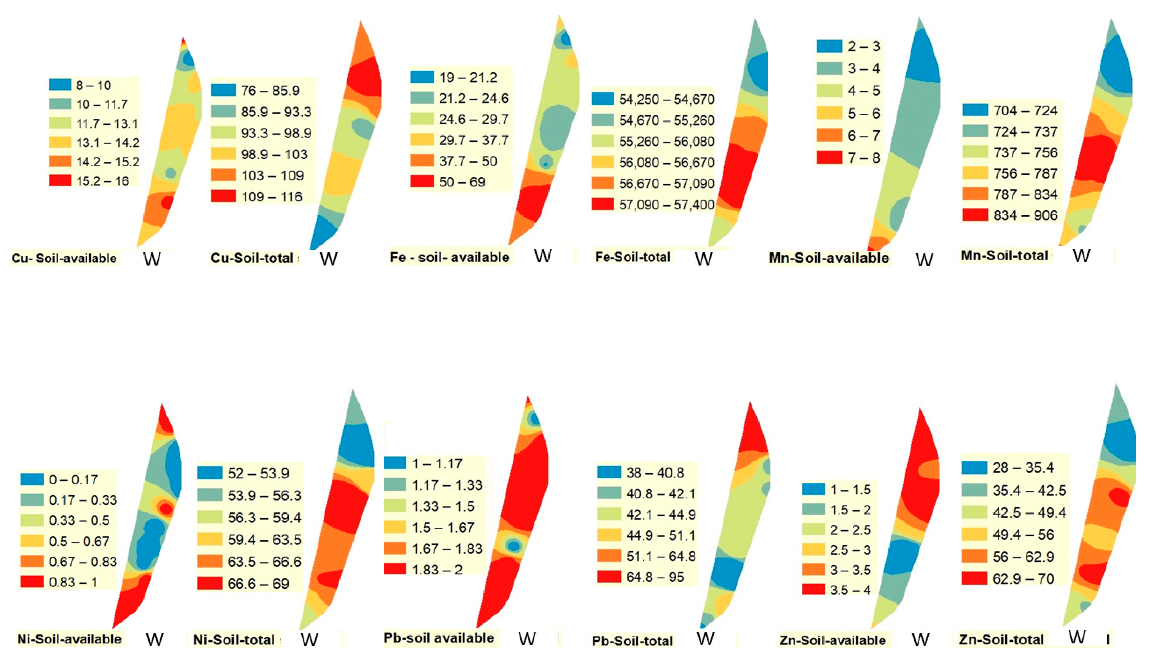
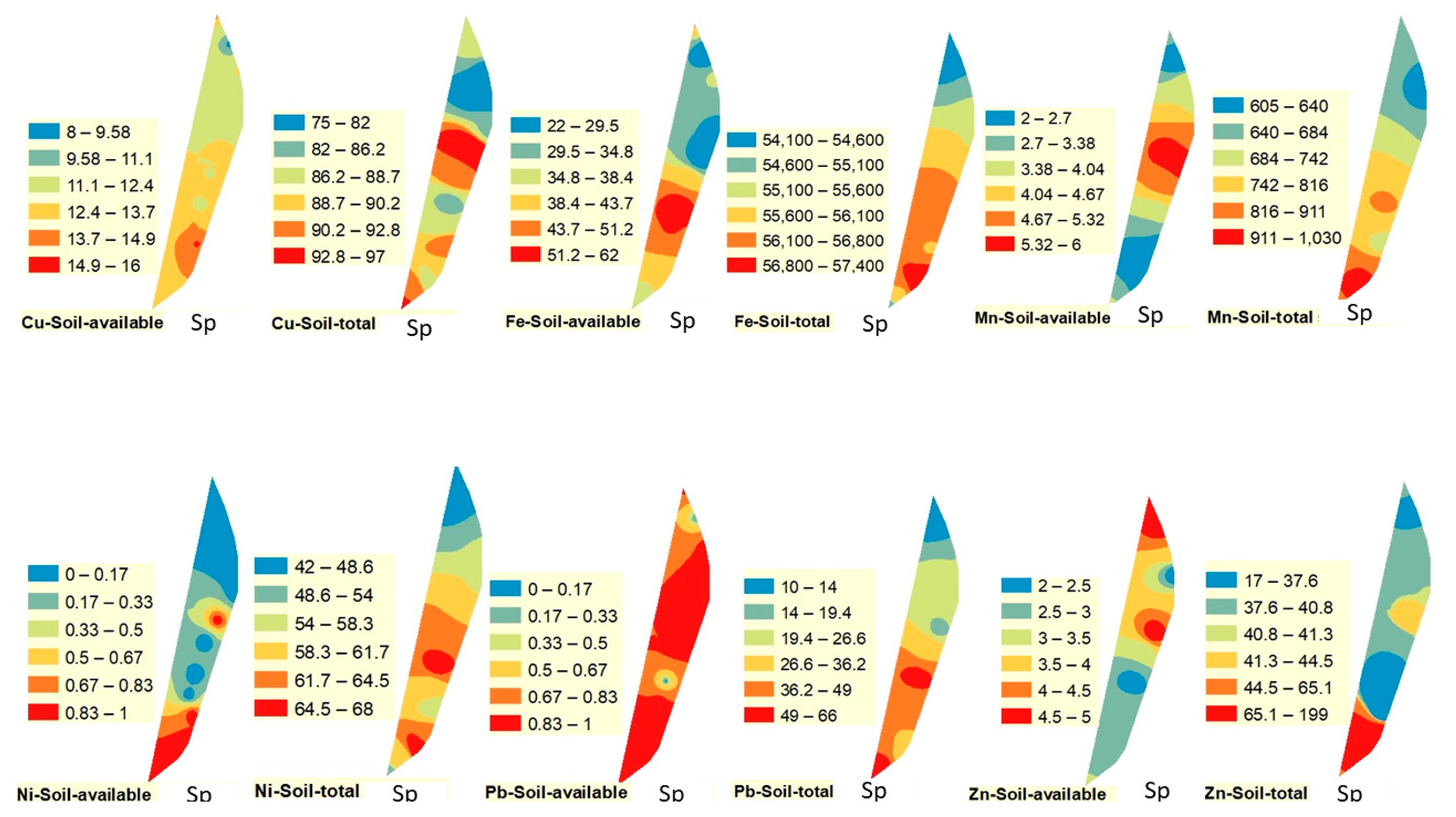
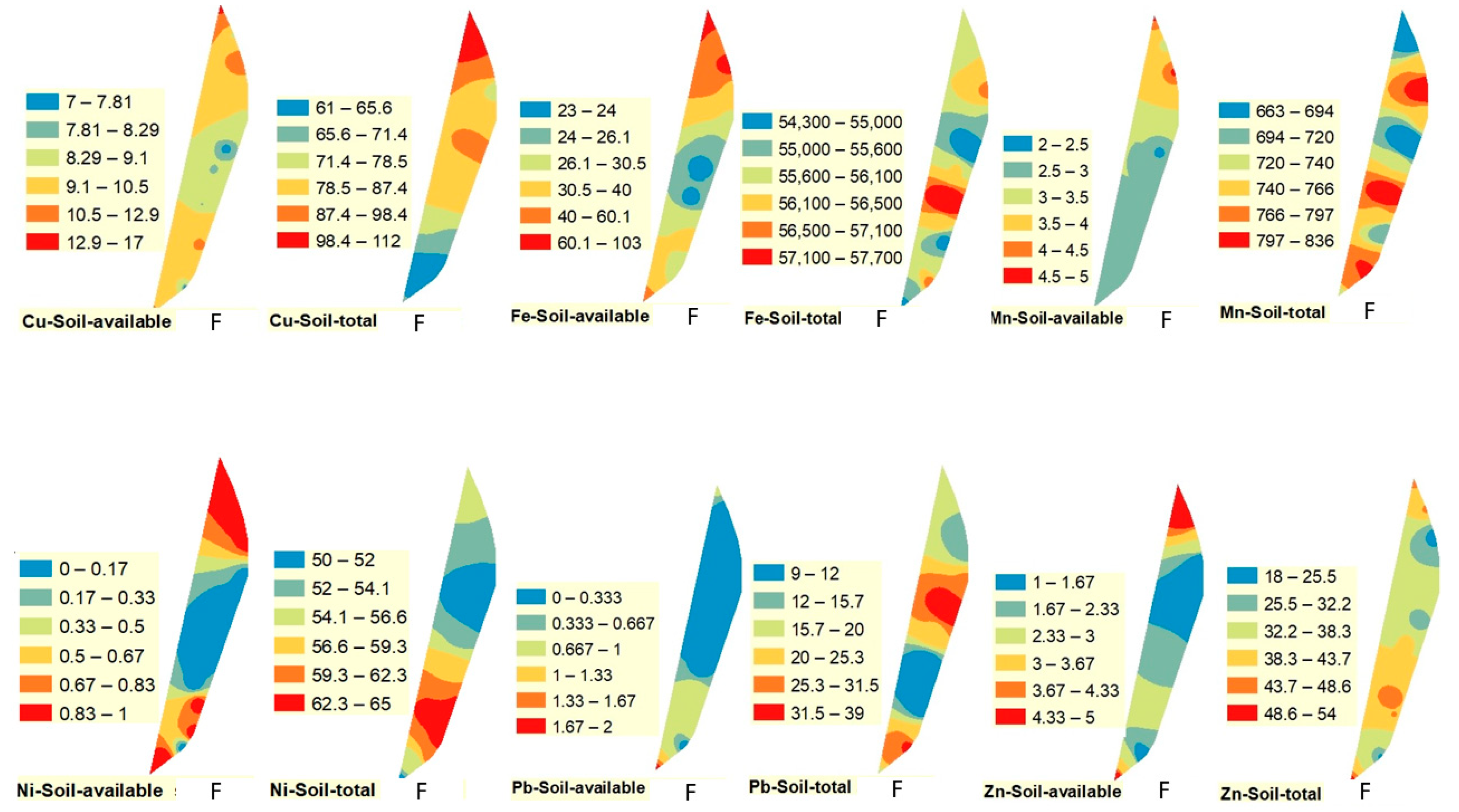
, where Cu correlated significantly (at p = 0.05) with SOM and CaCO₃. SOM plays a significant role in the mobility of metallic cations through complexation reactions that can modify the accumulation and toxicity of trace metals [42]. Available Cu followed a different behavioral pattern than the other studied available TEs in terms of variation among the locations. The spatial distribution of soil available heavy metals in the three seasons are shown in Figure 2, Figure 3 and Figure 4. The spatial distribution of Cu (available and total) followed a different pattern than Pb and Fe. The highest value of available Cu was observed in the southern part of the drain in winter and spring, while it was observed in the northern part of the drain in fall. On the other hand, the highest value of total Cu was recorded in the northern part of the drain in winter and fall and in the middle portion of the drain in spring.

Available Fe was not significantly higher in the fall, with a mean value of 41.89 mg kg⁻¹ and very high variation among locations (Table 2). Differences in total Fe were not significant between seasons; however, the highest value was recorded in the winter (Table 2). Although the total Fe values were much higher than available ones, the variation among locations was low. The mean concentrations of total Fe in the three seasons were higher than the average for world soils [28]. Soil properties may affect total Fe, as it is significantly correlated with pH and P (Table 3). Total Fe was also highly correlated with total Ni, whereas available Fe was highly correlated with available Cu (Table 3). Inter-element relationships offer information on the sources of the metals and their pathways [48]. The highest values of available and total Fe followed similar patterns in both winter and spring, when they were found in the southern part of the drain. On the other hand, the highest value of available Fe in the fall was observed in the north, while the highest value of total Fe in fall was in the middle part of the drain (Figure 2, Figure 3 and Figure 4).

Available Mn values varied between the seasons, with the highest values recorded in winter (Table 2). The available Mn was significantly different between winter and spring, however, the difference between spring and fall was not significant. There were no significant differences in the total values of Mn between seasons. Mean total Mn values were higher than the world average based on Kabata-Pendias [28]. Total Mn was significantly correlated with the soil properties pH, SOM, BD and N (Table 3). Total Mn was also significantly correlated with available Pb. This may indicate the same origin or same controlling factors for these metals in the analyzed soils [48]. The variation in Mn values among the locations was moderate in winter and fall, while it was high in spring as indicated by the CV values. The highest available values of Mn were recorded in the southern, middle and northern parts of the drain in winter, spring and fall, respectively (Figure 2, Figure 3 and Figure 4). On the contrary, the highest total values of Mn were observed in the middle and the southern parts of the drain in all studied seasons.

There was no significant difference in available Ni between the seasons (Table 2), but there was high variation in available Ni among the studied sites alongside the drain. The variation in total Ni between sites was moderate. The total and available Ni values followed similar patterns between seasons. The highest available and total Ni values were recorded in winter. The total Ni values were higher than the world soil average [28]. This could be attributed to soil use and management as suggested by Zhao et al. [45] or proximity to roads and automobiles, which can discharge high amounts of heavy metals [49,50]. The total Ni concentrations in our study are in the range of the maximum allowable concentration of Ni (20–60 mg kg⁻¹) stated by Kabata-Pendias [28]. Total Ni was correlated with the soil properties pH, SOM, BD and N (Table 3). Total Ni was also significantly correlated with available Pb and total Mn, indicating the possibility of the same source for these metals. The highest value of available Ni was observed in the northern and the southern parts of the drain with a tendency to be higher in the north during fall and in the south during spring (Figure 2, Figure 3 and Figure 4). Total concentration of Ni followed a similar pattern to some extent, being highest in the south in spring and fall and in the middle during winter.

Available Pb values varied significantly between seasons, with the highest level recorded in winter (Table 2). The variation of available Pb among the study sites was moderate in winter and spring, while it was high in fall. Variation in total Pb was high in all seasons. The total concentration of Pb also varied significantly between seasons, with the highest value recorded in winter, the same as available Pb. The mean concentrations of Pb found in this study were higher than the world soil average reported by Kabata-Pendias [28], and the mean total Pb concentrations were higher than the minimum limit (20–300 mg Kg⁻¹) given by Kabata-Pendias [28]. This could be attributed to proximity of the studied soil to the drain. The Kitchener Drain is known to carry Pb and other elements from agriculture, industry and roads. The only correlations between soil properties and total Pb were with SOM and BD (Table 3). The correlations between Pb concentrations and SOM content obtained in this study agree with the findings of Xun and Xuegang [48], who also indicated that SOM content had an essential role in the control of Pb sorption by soils. Furthermore, Pb was significantly correlated with total Mn and total Ni in our study. The highest values of available Pb were observed along the drain in winter and spring, while in fall, the highest value was observed in the southern part of the drain. Total Pb patterns differed from those of available Pb in the three studied seasons. Total Pb was highest in the northern, southern, and the middle parts of the drain in winter, spring and fall, respectively. The source of Pb in soil is often leaded gasoline [10]. In Kitchener Drain, this could result from running leaded gasoline in irrigation engines along the drain and in vehicles passing on nearby roads.

Available Zn varied significantly between winter and spring, as well as between spring and fall (Table 2). However, the mean values of total Zn did not show significant differences between seasons. The highest available and total Zn concentrations were recorded in the spring. Unlike most of the other TEs investigated in this study, Zn was lower than the world soil average and the maximum allowable Zn concentrations reported by Kabata-Pendias [28]. Total Zn did not correlate with any of the soil properties (Table 3). This is contrary to the findings of Xun and Xuegang [48], who found that Zn was negatively correlated with pH. Khaledian et al. [43] found a positive correlation between exchangeable Zn and both pH and total organic carbon, and a positive correlation between total Zn and total organic carbon. In this study, total Zn was significantly correlated with available Ni and available Zn. This implied that they may have the same source. The highest value of available Zn was observed in the northern part of the drain in all seasons, while the highest value of total Zn was observed toward the southern part of the drain in all seasons. The measured TEs exhibited wide differences from one site to another. This may be related to anthropogenic sources within the heavily inhabited and industrialized areas surrounding the study area.

Generally, total Fe, Mn, Ni, and Zn followed similar patterns in the winter. Total Fe, Mn, Ni, and Pb followed similar patterns in the spring, while total Ni and Mn only followed the same pattern in the fall. This indicated that Ni and Mn may have the same source in all seasons, while they share mutual sources with Fe and Zn in winter and with Fe and P in fall, which indicates that the season has a role in changing the variability of these elements. The spatial and seasonal distribution of elements in the study area clearly illustrate that some TEs increase toward the northern part of the drain that is located close to the Mediterranean Sea, such as total Cu, total and available Pb and available Zn in winter; available Pb and available Zn in spring; and total and available Cu, available Fe, available Ni, and available Zn in fall. Nethaji et al. [5] found metals increased toward the coast in their study area. They attributed this enrichment in TEs to anthropogenic activities. Najamuddin et al. [18] found that the seasons effect environmental physico-chemical characteristics differentially. They also confirmed that changes in environmental parameters such as temperature, pH, and redox potential (Eh) could influence elemental release from the solid soil phase to the liquid phase. This converted the sediments from an element sink to an elemental source for the overlying waters. The Kitchener Drain flows through highly fertile and densely populated areas (Garbia and Kafr El-Sheikh governorates) in the Nile Delta, Egypt. It carries fertilizers from agricultural activities conducted beside the drain, urban and sewage effluents, and industrial effluents from textiles industries in Mahala Al-kobra, Garbia. The drain is cleared in the winter, and the dredged sediment is moved onto the land on either side of the drain. The people there work the sediment gradually into their soils because they think this will be beneficial to their soils. However, this creates a high risk of heavy metals’ contamination in their soils. This management of dredged materials is probably the main reason for high average TEs contents and high variations in TEs between seasons. Zhao et al. [45] explained that the application of sediments into soil has played a very important role in many agricultural civilizations such as China because the dredged sediments contain high levels of SOM and can improve soil quality and crop production. However, trace metals may accumulate to toxic levels in agricultural soils over time through the application of polluted sediments. In addition, many workers have studied elemental pollution in settings such as marine, fluvial, drains, and estuarine environments and found variation in the distribution of heavy metals. Ali et al. [8] reported accumulation of TEs in soil that resulted from continuous irrigation with polluted water. The relatively low concentration of TEs at some locations in the study area is probably due to the soil characteristics [51] and tidal effects in the Kitchener Drain, which flush the finer particles into deeper regions [5].

Our results were generally similar to those of Chen et al. [52], who reported that Cu, Fe, Mn, Ni, Pb, and Zn concentrations decreased with distance from the drainage canal in three short sediment cores sampled from Burullus Lake. Our results for total and available TE concentration were higher than those from some other studies in the Nile Delta, such as Elkady et al. [16], who studied TEs in sediment samples collected from Lake Manzala, Egypt. Our TE concentrations were also higher than background values recorded by Melegy et al. [53] in 24 soil samples from the El-Tabbin region (Great Cairo, Egypt). Elbana et al. [54], when studying agricultural soils near Cairo, Egypt, found available TE concentrations (AB-DTPA) in soils for Cu (0.9–42.3 mg kg⁻¹), Ni (0.2–4.1 mg kg⁻¹), and Pb (0.5–20.0 mg kg⁻¹) that tended to be higher than the levels found in this study. However, Elbana et al. [54] reported total TEs concentrations for Cu (1.6–120.5 mg kg⁻¹), Ni (0.2–31.3 mg kg⁻¹), and Pb (7.0–50.0 mg kg⁻¹) that tended to be lower than the total concentrations found in this study, as did Khalil et al. [55] who reported total TEs as Cu (23–57.8 mg kg⁻¹), Ni (12.3–53.3 mg kg⁻¹), and Pb (8–36 mg kg⁻¹) in sediments from Burullus Lagoon, Egypt.

3.3. Plant Tissue Concentration of PTEs

The N and K data showed higher levels (min, max and mean values) in winter than other seasons while P was highest in the spring (

Table 4. Descriptive statistics for trace elements in plant tissues collected from the study area.

	Cu	Fe	Mn	Ni	Pb	Zn	K	P	N
	mg kg−1
Winter
Mean	7.53 a,*	1284.1 a	22.65 a	ND	0.47 a	20.29 a	38,448.3 a	66.0 b	3267.97 a
Max	18.75	2331.0	38.21	ND	3.55	27.95	71,375.0	189.36	5026.0
Min	1.72	403.0	11.52	ND	ND	12.00	21,700.0	31.56	1200.0
SD	4.72	588.23	7.90	-	1.07	6.11	13,038.1	43.17	1182.94
CV	62.75	45.81	34.90	-	228.30	30.11	33.91	65.43	36.2
Spring
Mean	2.67 b	120.51 b	12.19 b	ND	ND	18.13 a	33,248.7 a	855.0 a	2874.47 a
Max	10.11	184.01	22.01	ND	ND	64.65	64,078.0	3542.0	5224.0
Min	ND	9.61	6.95	ND	ND	5.90	8294.5	42.0	602.0
SD	3.23	45.22	4.11	-	-	21.15	18,706.1	1217.75	1461.83
CV	121.15	37.53	33.69	-	-	116.64	56.26	142.43	50.86
Fall
Mean	0.93 b	87.59 b	7.52 c	ND	ND	10.57 b	20,889.8 b	79.4 b	2695.0 a
Max	5.70	358.15	19.50	ND	ND	19.90	63,825.0	147.28	4802.0
Min	ND	15.95	1.70	ND	ND	3.70	682.5	31.56	1134.0
SD	1.41	64.69	4.26	-	-	6.17	18,002.6	25.38	1074.76
CV	152.20	73.86	56.62	-	-	58.32	86.18	31.95	39.88

nd: non-detected; * Different letters in each column of the table indicate significant differences at p < 0.05 (based on Duncan test) between studied seasons.

). This is because of fertilization and legumes cultivation in this season in the northern Nile Delta region. Our results also generally indicated that TEs concentrations differed significantly between seasons, with most metals being higher in the winter compared to spring and fall (Table 4). The increase in TEs during the winter may be attributed to non-leaching of metals from the soil because of shortage in irrigation water in the river and canals during the winter due to reduced allocations of water for irrigation.

The plant tissue concentrations of the studied TEs was under the critical concentration levels according to Kabata-Pendias [28]. There was a significant (p < 0.05) difference between seasons in all the studied TEs (Table 4). The presence of an element in soil does not imply that it is available to plants, particularly if they are insoluble in the soil solution (Chojnacka et al. [56].

3.4. Water PTEs Soluble Concentrations

Basic water quality parameters varied between seasons. Salinity decreased during spring and increased during the winter and fall seasons. The contents of dissolved salts in the water followed the following sequence: Na > Cl > HCO₃ > Ca > Mg > SO₄ > K. The maximum amount of available N was recorded in winter while the maximum amount of available p was recorded in the fall. Our observations were in agreement with Younes and Nafea [57], who studied fifteen surface water samples collected seasonally from Lake Burullus.

Trends in TEs concentrations in the drain water are shown in

Table 5. Descriptive statistics for trace elements dissolved in river water at the study area.

	pH	EC	K	Na	Ca	Mg	HCO3	Cl	SO4	P	N	Fe	Mn	Zn
	mg L−1
Winter
Mean	7.26 b,*	1.46 b	0.46 b	7.5 4a	3.80 a	3.40 b	6.43 b	6.66 a	2.11 a	1.44 b	61.04 a	nd	nd	21.87 a
Max	7.65	1.68	0.51	9.00	4.40	4.20	7.00	8.40	2.89	2.20	71.30	nd	nd	43.38
Min	7.17	1.25	0.43	5.96	3.20	2.00	6.00	4.80	0.28	1.17	54.50	nd	nd	6.65
SD	0.12	0.16	0.03	0.99	0.37	0.45	0.25	1.28	0.64	0.32	4.86	-	-	13.45
CV	1.62	10.67	5.51	13.18	9.74	13.25	3.94	19.19	30.11	22.02	7.96	-	-	61.49
Spring
Mean	7.19 c	1.22 c	0.51 a	6.47 a	2.63 b	3.24 b	5.74 c	4.60 b	1.68 b	1.43 b	22.13 b	0.51 a	2.05 a	20.48 a
Max	7.50	1.88	0.66	11.54	3.40	4.80	8.40	8.60	2.56	2.90	30.80	1.33	21.00	41.13
Min	7.05	0.64	0.34	2.45	2.00	2.00	3.60	1.80	0.59	0.40	14.00	-	-	6.42
SD	0.13	0.38	0.10	2.74	0.48	0.77	1.50	2.04	0.53	0.85	5.11	0.48	5.98	13.86
CV	1.80	31.49	18.94	42.30	18.37	23.91	26.21	44.30	31.22	59.35	23.11	95.27	291.26	67.66
Fall
Mean	7.39 a	1.87 a	0.45 b	7.54 a	3.85 a	3.81 a	7.76 a	7.35 a	0.47 c	2.07 a	22.20 b	0.34 a	0.17 b	23.26 a
Max	7.49	2.48	0.57	11.55	4.80	4.60	10.40	10.50	1.58	3.65	30.80	1.76	0.33	64.43
Min	7.28	1.50	0.38	5.60	3.00	2.80	7.00	5.20	0.14	1.35	16.80	-	-	6.88
SD	0.07	0.33	0.05	1.91	0.43	0.45	1.07	1.95	0.39	0.75	3.84	0.51	0.12	19.04
CV	0.89	17.50	11.89	25.28	11.27	11.80	13.84	26.57	81.99	36.32	17.30	149.73	70.23	81.88

nd: non-detected. * Different letters in each column indicate significant differences at p < 0.05 (based on Duncan test) between studied seasons.

. Copper and Pb were not detectable (ND) in all seasons and therefore do not appear in Table 5. Iron was ND in winter and the Sp and F differences were not significant. The highest value of Fe was 1.1 mg L⁻¹ in the middle and northern portions of the drain, while the lowest value was ND the southern portion. Soluble Fe in the water was higher than the average global concentrations of dissolved Fe (i.e., 0.67, 0.04, 0.06, or 0.087 mg L⁻¹) in rivers according to Gordeev and Lisitzin [44]. Manganese concentrations were significantly different among the samples (Table 5) and were higher than the average global concentration of dissolved Mn (i.e., 0.01, 0.012, 0.082 or 0.034 mg L⁻¹) in rivers [44]. The Mn trend was similar to Fe where the highest values were in the northern portion of the drain and the lowest values in the southern part. The highest value was 0.3 mg L⁻¹, whereas the lowest value was ND. In winter, Fe concentration was also different among the locations. The highest Fe reading was 1.2 mg L⁻¹ in the middle portion of the drain and the lowest value was ND in the southern portion. The mean values of Fe and Mn tended to be higher in spring, but the spring Fe value was not significantly different from the fall value. Dissolved Zn was not significantly different between seasons, and it was higher than the average global concentrations (i.e., 0.02, 0.01, 0.03, 0.0006 or 0.00074 μg L⁻¹) in rivers according to Gordeev and Lisitzin [44].

4. Ecological Risk Assessment

Assessment of soil contamination is considered crucial for evaluating the health of ecosystems; however, the determination of element concentrations alone is not enough to assess possible anthropogenic and health impacts. Thus, several quantitative indices have been developed to assess the level of pollution and ecological risk posed by TEs in the environment [58]. Availability ratios are element availability indices normalized for the total element concentrations to represent the percentage of the available fraction of an element’s total concentration in soil. This decreases the impact of the geogenic influence on these availability indices, which makes them more sensitive to human-induced pollution sources [29]. The study trend was for Cu to have the highest AR values (ranged from 8.01 to 18.4%) while the lowest AR values were for Fe (0.03 to 0.19%) (Figure 5). However, there were differences in AR between seasons. The availability of TEs in soil is mainly affected by factors such as pH and organic matter content [43], this could lead to different AR values in different seasons even under the same anoxic conditions and total metal amounts [29].

The enrichment factor (EF) is an integrated pollution load index and is useful to assess soil environmental quality. The mean enrichment factor (EF) values for various metals were between Class I and Class II enrichment (Figure 5) (

Table 6. The criteria for the various ecological risk assessment indices used in this study.

Indices	Class	Degree	Reference
BAF	≤6	Low degree of contamination	(Hakanson 1980) [33]
	6–12	Moderate degree of contamination
	12–24	Considerable degree of contamination
	>24	Very high degree of contamination
CF	CF < 1	Low contamination factor	(Hakanson 1980) [33]
	1 ≤ CF< 3	Moderate contamination factor
	3 ≤ CF < 6	Considerable contamination factor
	CF ≥ 6	Very high contamination factor
EF	EF < 1	No enrichment	(Chen et al. 2007; Sakan et al. 2009) [59,60]
	1 < EF < 3	Minor enrichment
	3 < EF < 5	Moderate enrichment
	5 < EF < 10	Moderately severe enrichment
	10 < EF < 25	Severe enrichment
	25 < FE < 50	Highly severe enrichment
	EF > 50	extremely severe
Igeo	Igeo ≤ 0	Uncontaminated	(Muller 1981) [61]
	0 to Igeo ≤ 1	Uncontaminated to moderately contaminated
	1to Igeo ≤ 2	Moderately contaminated
	2 to Igeo ≤ 3	Moderately to heavily contaminated
	3 to Igeo ≤ 4	Heavily contaminated
	4 to Igeo ≤ 5	Heavily to extremely contaminated
	≤5 Igeo	Extremely contaminated

). A value of 0.5 < EF < 1.5 indicates that the elements are completely from crustal sources (e.g., weathering products), whereas an EF value > 1.5 indicates that a considerable proportion of the element is supplied from non-crustal sources (e.g., biota and/or polluted drainage) [30]. The maximum mean EF values belonged to Cu in all three seasons, and 19 of the 21 EF values were >1.5, indicating likely anthropogenic pollution. This supports the possibility that Cu has been enriched by agricultural, urban, and industrial discharges into the drain. None of the other TEs investigated had EF values that indicated anthropogenic pollution (Figure 5).

The geo-accumulation index (Igeo) was calculated to determine the degree of contamination in each soil sample. The Igeo values were in class 1 (between 0 and 1) for all the assessed TEs (Figure 5), which indicates uncontaminated to moderately contaminated soils [62] (Table 6). The contamination factor (CF) values were in the low, moderate, and considerable contamination ranges (Table 6). Maximum mean CF values were in the order of Cu > Ni > Fe > Mn > Pb > Zn. The CF values for Cu were higher than those for all other studied TEs at all sampling locations (Figure 5), which was similar to the EF and Igeo results. The CF values provided support for at least moderate soil contamination by all TEs studied except Zn. In general, all sites possessed low degrees of contamination. In addition, the values of PLI indicated that all the soils were uncontaminated, which was in agreement with Baz and Khalil [63] in their study of 10 sites along the central zone of the Egyptian Mediterranean coast.

In an attempt to study TEs mobility from soil to plant, and thus to assess the biohazard related to the observed TE levels, soil-to-plant TC was calculated (Figure 6). The TC values followed the decreasing order Mn > Zn > Cu > Fe, while Pb and Ni were ND. The transfer factor for Mn ranged from 0.16 to 1.34 followed by Zn, which ranged from 0.11 to 1.37. Zn and Mn may not pose a risk to human health because these metals are among the essential elements for humans [64]; however, these are also micronutrients and if they are present in concentrations above their optimal range they can cause health problems [65]. The values of TC are reported to have an inversely proportional relationship with element sorption [31].

The mean bioaccumulation factor (BAF) from the soil to plant was greater than unity for all of the TEs and had the following order: Mn > Fe > Zn > Cu, with the other studied TEs being ND (Figure 6). Mn had the highest BAF ranges (6.87 to 85.3) followed by Fe (0.91 to 85.4), while Zn had the lowest ranges (1.3 to 35.5) in all locations and all three seasons. In our study the winter was higher for Mn, Fe and Zn; while the fall was higher for Mn and Zn. This probably reflects the absorption of pollutants from the sewage outlets nearby and also the accumulation of plant litter [66].

Principal Component Analysis (PCA)

The PCA was performed to further assist the identification and analysis of sources of heavy metals in soil. First, the results of Kaiser–Meyer–Olkin (KMO = 0.621) and significance Bartlett’s sphericity tests was p = 0.007 (less than 0.01), which generally indicated that total and available trace elements concentrations in surface soil around Kitchener Drain were suitable for PCA. The PCA is used to reduce several potential indicators to a smaller set of comprehensive ones. It is also used to further evaluate the relationships between and sources of the metals [67]. The results of PCA analysis in this study were used to assist the source identification of trace elements and are shown in

Table 7. Total variance explained and rotated component matrix (four principal components selected) for TE contents.

Component	Initial Eigenvalues				Rotated Component Matrix
	Total	% of Variance	Cumulative %	Metals	PC1	PC2	PC3	PC4
1	3.15	26.22	26.22	Cu T *	0.03	0.76	0.52	0.11
2	2.97	24.75	50.97	Fe T	0.01	0.70	0.03	0.10
3	1.58	13.15	64.12	Mn T	−0.02	0.23	0.05	0.90
4	1.28	10.68	74.80	Ni T	0.09	0.84	−0.06	0.27
5	0.79	6.56	81.36	Pb T	0.18	0.35	0.59	0.46
6	0.64	5.37	86.73	Zn T	−0.44	0.70	0.03	−0.20
7	0.54	4.51	91.24	Cu A **	−0.11	0.23	0.77	−0.20
8	0.38	3.15	94.40	Fe A	0.86	−0.12	−0.03	0.11
9	0.29	2.40	96.80	Mn A	0.86	−0.09	0.14	−0.11
10	0.19	1.56	98.36	Ni A	0.85	0.03	−0.03	0.11
11	0.11	0.93	99.29	Pb A	0.08	−0.22	0.78	0.17
12	0.09	0.71	100.00	ZnA	0.70	0.38	−0.01	−0.46

* T; total heavy metals concentration, ** A; available heavy metals concentration.

. Based on eigenvalues (eigenvalue > 1), the majority of variance (74.8%) of the scaled data was explained by four principal eigenvectors. The first, PC1, explained 26.2% of the total variance and was strongly and positively related to available Fe, Mn, Ni and Zn. The second, PC2, explained 22.8% of the total variance and showed highly positive factor loadings for total Cu, Fe, Ni, and Zn. The third, PC3, explained 13.2% of the total variance and showed highly positive factor loadings for Pb. The fourth, PC4, explained 12.6% of the total variance and showed highly positive factor loadings for total Mn. These degrees of covariance are strongly suggestive of common sources for the metals. Therefore, total Cu, Fe, Ni and Zn all corresponded to each other, indicating that they might have the same source, while the available forms of Fe, Mn, Ni and Zn might also come from the same source.

There are several studies that have shown that the association of these trace elements using PC analysis can be indicative of anthropogenic activities or diagenetic processes [39]. Fe and Mn are well known to largely be geogenic [68], while the various industrial activities and agrochemicals used in and around Kitchener Drain may contribute to the concentrations of Cu, Ni, Pb and Zn. The concentrations of total and available elements exhibited clear differences among the three seasons and represent clear evidence of accumulation and mobilization of trace elements in soils.

5. Conclusions

This work provides the first comprehensive analysis of TEs bioavailability in surface soil, water and plant tissues around Kitchener Drain near the Nile Delta coast. The results indicated high concentrations of some TEs around Kitchener Drain in soil and plant samples, especially in winter and in the southern parts around the drain. However, water sample concentrations of these elements were lower because of bonding of these elements with sediment in the drain. The risk assessment indices indicated that some elements, especially Cu, are from anthropogenic sources, which indicates a higher risk of additional accumulation from such sources in the future. The determination of TEs concentrations in the soils and plants around Kitchener Drain is a significant step toward assessment of ecological risks in this area of Egypt due to its proximity to the polluted drain. This study should help decision makers consider this area in agricultural development plans and pollution prevention and remediation. However, this study had a fairly limited number of samples, which introduces a level of uncertainly to the results. More studies regarding biological monitoring and pollution in food chains should be performed in the future.

References

1. Zhu, J.; Zhang, J.; Li, Q.; Han, T.; Xie, J.; Hua, Y.; Chai, L. Phylogenetic analysis of bacterial community composition in sediment contaminated with multiple heavy metals from the Xiangjiang River in China. Mar. Pollut. Bull. 2013, 70, 134–139. [Google Scholar] [CrossRef] [PubMed]
2. Oliver, M.A.; Gregory, P.J. Soil, food security and human health: A review. Eur. J. Soil. Sci. 2015, 66, 257–276. [Google Scholar] [CrossRef]
3. Sun, X.; Fan, D.; Liu, M.; Tian, Y.; Pang, Y.; Liao, H. Source identification, geochemical normalization and influence factors of heavy metals in Yangtze River Estuary sediment. Environ. Pollut. 2018, 241, 938–949. [Google Scholar] [CrossRef] [PubMed]
4. Salas, P.M.; Sujatha, C.H.; Kumar, C.S.R.; Cheriyan, E. Heavy metal distribution and contamination status in the sedimentary environment of Cochin estuary. Mar. Pollut. Bull. 2017, 119, 191–203. [Google Scholar] [CrossRef] [PubMed]
5. Nethaji, S.; Kalaivanan, R.; Viswam, A.; Jayaprakash, M. Geochemical assessment of heavy metals pollution in surface sediments of Vellar and Coleroon estuaries, southeast coast of India. Mar. Pollut. Bull. 2017, 115, 469–479. [Google Scholar] [CrossRef] [PubMed]
6. El Azhari, A.; Rhoujjati, A.; El Hachimi, M.L.; Ambrosi, J. Pollution and ecological risk assessment of heavy metals in the soil-plant system and the sediment-water column around a former Pb/Zn-mining area in NE Morocco. Ecotoxicol. Environ. Saf. 2017, 144, 464–474. [Google Scholar] [CrossRef] [PubMed]
7. Motoshita, M.; Ono, Y.; Pfister, S.; Boulay, A.M.; Berger, M.; Nansai, K.; Tahara, K.; Itsubo, N.; Inaba, A. Consistent characterisation factors at midpoint and endpoint relevant to agricultural water scarcity arising from freshwater consumption. Int. J. Life Cycle Assess. 2018, 23, 2276–2287. [Google Scholar] [CrossRef]
8. Ali, H.M.; EL-Mahrouk, E.M.; Hassan, F.A.; EL-Tarawy, M.A. Usage of sewage effluent in irrigation of some woody tree seedlings. Part 3: Swieteniamahagoni (L.) Jacq. Saudi J. Biol. Sci. 2011, 18, 201–207. [Google Scholar] [CrossRef] [PubMed]
9. Saeed, S.M.; Shaker, I.M. Assessment of heavy metals pollution in water and sediments and their effect on Oreochromis Niloticus in the Northern Delta Lakes, Egypt. In Proceedings of the 8th International Symposium on Tilapia in Aquaculture, Cairo, Egypt, 12 October 2008; Volume 475, p. 490. [Google Scholar]
10. Oliveira, A.; Palma, C.; Valenca, M. Heavy metal distribution in surface sediments from the continental shelf adjacent to Nazare canyon. Deep Sea Res. II 2011, 58, 2420–2432. [Google Scholar] [CrossRef]
11. Maas, S.; Scheifler, R.; Benslama, M.; Crini, N.; Lucot, E.; Brahmia, Z.; Benyacoub, S.; Giraudoux, P. Spatial distribution of heavy metal concentrations in urban, suburban and agricultural soils in a Mediterranean city of Algeria. Environ. Pollut. 2013, 158, 2294–2301. [Google Scholar] [CrossRef]
12. Krishna, A.K.; Govil, P.K. Heavy metal distribution and contamination in soils of Thane–Belapur industrial development area, Mumbai, Western India. Environ. Geol. 2013, 47, 1054–1061. [Google Scholar] [CrossRef]
13. Islam, S.; Ahmed, K.; Raknuzzaman, M.; Al-Mamun, H.; Kamrul Islam, M. Heavy metal pollution in surface water and sediment: A preliminary assessment of an urban river in a developing country. Ecol. Indic. 2015, 48, 282–291. [Google Scholar] [CrossRef]
14. El-Badry, A.E.A.; El-Kammar, A.M. Spatial distribution and environmental geochemistry of zinc metal in water and surficial bottom sediments of Lagoon Burullus, Egypt. Mar. Pollut. Bull. 2018, 127, 811–816. [Google Scholar] [CrossRef] [PubMed]
15. Fawzy, M.A.; Badr, N.E.; El-Khatib, A.; Abo-El-Kassem, A. Heavy metal biomonitoring and phytoremediation potentialities of aquatic macrophytes in River Nile. Environ. Monit. Assess. 2012, 184, 1753–1771. [Google Scholar] [CrossRef] [PubMed]
16. Elkady, A.A.; Sweet, S.T.; Wade, T.L.; Klein, A.G. Distribution and assessment of heavy metals in the aquatic environment of Lake Manzala, Egypt. Ecol. Indic. 2015, 58, 445–457. [Google Scholar] [CrossRef]
17. EEAA. Egyptian State of the Environment Report; Egyptian Environmental Affairs Agency: Cairo, Egypt, 2008.
18. Najamuddin, P.T.; Sanusi, H.S.; Nurjaya, I.W. Seasonal distribution and geochemical fractionation of heavy metals from surface sediment in a tropical estuary of Jeneberang River, Indonesia. Mar. Pollut. Bull. 2016, 111, 456–462. [Google Scholar] [CrossRef]
19. Elbehiry, F.; Mahmoud, M.A.; Negm, A. Land Use in Egypt’s Coastal Lakes: Opportunities and Challenges. In Egyptian Coastal Lakes and Wetlands: Part I Characteristics and Hydrodynamics, The Handbook of Environmental Chemistry; Negm, A.M., Bek, M.A., Abdel Fattch, S., Eds.; Springer: Berlin/Heidelberg, Germany, 2018; pp. 21–36. [Google Scholar] [CrossRef]
20. Van der Most, H.; Marchand, M.; Bucx, T.; Nauta, T.; van Staveren, M. Towards Sustainable Development of Deltas, Estuaries and Coastal Zones. Description of Eight Selected Deltas. 2018. Available online: http://www.delta-alliance (accessed on 20 December 2018).
21. Elbasiouny, H.; Abowaly, M.; Abu-Alkheir, A.; Gad, A. Spatial variation of soil carbon and nitrogen pools by using ordinary kriging method in an area of north Nile Delta, Egypt. CATENA 2014, 113, 70–78. [Google Scholar] [CrossRef]
22. Sparks, D.L.; Page, A.L.; Helmke, P.A.; Loppert, R.H.; Soltanpour, P.N.; Tabatabai, M.A.; Johnston, C.T.; Summner, M.E. Methods of Soil Analysis: Chemical Methods, Part 3; ASA and SSSA: Madison, WI, USA, 1996; pp. 1201–1230. [Google Scholar]
23. Blake, G.R.; Hartge, K.H. Bulk density, In Methods of Soil Analysis. Part 1, 2nd ed.; Klute, A., Ed.; ASA and SSSA: Madison, WI, USA, 1986; Volume 9, pp. 363–375. [Google Scholar]
24. Page, A.L.; Miller, R.H.; Baker, D.E. Methods of Soil Analysis-Part 2—Chemical and Microbiological Properties, 2nd ed.; Soil Science Society of America: Madison, WI, USA, 1982; p. 1159. [Google Scholar]
25. USEPA. Test Methods for Evaluating Solid Waste Physical, Chemical Methods; US Environmental Protection Agency, USEPA: Washington, DC, USA, 1996; p. SW-846.
26. APHA. Standard Methods for the Examination of Water and Waste Water, 22nd ed.; American Public Health Association, American Water Works Association, Water Environment Federation: Washington, DC, USA, 2012. [Google Scholar]
27. Jones, J.B., Jr.; Wolf, B.; Mills, H.A. Plant Analysis Handbook; Micro-Macro Publishing, Inc.: Athens, Greece, 1991. [Google Scholar]
28. Kabata-Pendias, A. Trace Elements in Soils and Plants; CRC Press: Boca Raton, FL, USA, 2011. [Google Scholar]
29. Massas, I.; Ehaliotis, C.; Kalivas, D.; Panagopoulou, G. Concentrations and availability indicators of soil heavy metals; the case of children’s playgrounds in the city of Athens (Greece). Water Air Soil Pollut. 2010, 212, 51–63. [Google Scholar] [CrossRef]
30. Zhang, J.; Liu, C.L. Riverine composition and estuarine geochemistry of particulate metals in China—Weathering features, anthropogenic impact and chemical fluxes. Estuar. Coast. Shelf Sci. 2002, 54, 1051–1070. [Google Scholar] [CrossRef]
31. Antoniadis, V.; Shaheen, S.M.; Boersch, J.; Frohne, T.; Laing, G.D.; Rinklebe, J. Bioavailability and risk assessment of potentially toxic elements in garden edible vegetables and soils around a highly contaminated former mining area in Germany. J. Environ. Manag. 2017, 186, 192–200. [Google Scholar] [CrossRef]
32. Kasa, E.; Felix-Henningsen, P.; Duering, R.A.; Gjoka, F. The occurrence of heavy metals in irrigated and non-irrigated arable soils, NW Albania. Environ. Monit. Assess. 2014, 186, 3595–3603. [Google Scholar] [CrossRef] [PubMed]
33. Hakanson, L. An ecological risk index for aquatic pollution control: A sedimentological approach. Water Res. 1980, 14, 975–1001. [Google Scholar] [CrossRef]
34. Xu, D.; Zhou, P.; Zhan, J.; Gao, Y.; Dou, C.; Sun, Q. Assessment of trace metal bioavailability in garden soils and health risks via consumption of vegetables in the vicinity of Tongling mining area, China. Ecotoxicol. Environ. Saf. 2013, 90, 103–111. [Google Scholar] [CrossRef] [PubMed]
35. Jolly, Y.N.; Islam, A.; Akbar, S. Transfer of metals from soil to vegetables and possible health risk assessment. Springer Plus 2013, 2, 1–8. [Google Scholar] [CrossRef] [PubMed] [Green Version]
36. Ghosh, M.; Singh, S.P. A review on phytoremediation of heavy metals and utilization it’s by products. Appl. Ecol. Environ. Res. 2005, 3, 1–18. [Google Scholar] [CrossRef]
37. Wang, X.S.; Qin, Y. Accumulation, distribution and environmental risk of heavy metals in Xuzhou urban topsoil. Environ. Monit. Chin. 2006, 22, 70–75. [Google Scholar]
38. Li, S.; Zhang, Q. Risk assessment and seasonal variations of dissolved trace elements and heavy metals in the Upper Han River, China. J. Hazard. Mater. 2010, 181, 1051–1058. [Google Scholar] [CrossRef] [PubMed]
39. Wang, Y.; Yang, L.; Kong, L.; Liu, E.; Wang, L.; Zhu, J. Spatial distribution, ecological risk assessment and source identification for heavy metals in surface sediments from Dongping Lake, Shandong, East China. Catena 2015, 125, 200–205. [Google Scholar] [CrossRef]
40. Wang, C.; Liu, S.; Zhao, Q.; Deng, L.; Dong, S. Spatial variation and contamination assessment of heavy metals in sediments in the Manwan Reservoir, Lancang River. Ecotoxicol. Environ. Saf. 2012, 82, 32–39. [Google Scholar] [CrossRef]
41. Balkhair, K.S.; Ashraf, M.A. Field accumulation risks of heavy metals in soil and vegetable crop irrigated with sewage water in western region of Saudi Arabia. Saudi J. Biol. Sci. 2016, 23, S32–S44. [Google Scholar] [CrossRef] [PubMed]
42. Kennou, B.; El Meray, M.; Romane, A.; Arjouni, Y. Assessment of heavy metal availability (Pb, Cu, Cr, Cd, Zn) and speciation in contaminated soils and sediment of discharge by sequential extraction. Environ. Earth Sci. 2015, 74, 5849–5858. [Google Scholar] [CrossRef]
43. Khaledian, Y.; Pereira, P.; Brevik, E.C.; Pundyte, N.; Paliulis, D. The influence of organic carbon and pH on heavy metals, potassium, and magnesium levels in Lithuanian Podzols. Land Degrad. Dev. 2017, 28, 345–354. [Google Scholar] [CrossRef]
44. Gordeev, V.V.; Lisitzin, A.P. Geochemical interaction between the freshwater and marine hydrospheres. Russ. Geol. Geophys. 2014, 55, 562–581. [Google Scholar] [CrossRef]
45. Zhao, R.; Coles, N.A.; Wu, J. Status of heavy metals in soils following long-term river sediment application in plain river network region, southern China. J. Soils Sediments 2015, 15, 2285–2292. [Google Scholar] [CrossRef]
46. Guo, H.; Zhang, D.; Wen, D.; Wu, Y.; Ni, P.; Jiang, Y.; Guo, Q.; Li, F.; Zheng, H.; Zhou, Y. Arsenic mobilization in aquifers of the southwest Songnen basin, P.R. China: Evidences from chemical and isotopic characteristics. Sci. Total Environ. 2014, 490, 590–602. [Google Scholar] [CrossRef] [PubMed]
47. Rinklebe, J.; Du, L.G. Factors controlling the dynamics of trace metals in frequently flooded soils. In Dynamics and Bioavailability of Heavy Metals in the Root Zone; Selim, H.M., Ed.; CRC Press: Boca Raton, FL, USA, 2011; pp. 245–270. [Google Scholar]
48. Xun, Y.; Xuegang, L. Heavy Metals in Sediment from Bei Shan River: Distribution, Relationship with Soil Characteristics and Multivariate Assessment of Contamination Sources. Bull. Environ. Contam. Toxicol. 2015, 95, 56–60. [Google Scholar] [CrossRef] [PubMed]
49. Trujillo-González, J.M.; Torres-Mora, M.A.; Keesstra, S.; Brevik, E.C.; Jiménez Ballesta, R. Heavy metal accumulation related to population density in road dust samples taken from urban sites under different land uses. Sci. Total Environ. 2016, 553, 636–642. [Google Scholar] [CrossRef]
50. Tahir, M.; Iqbal, M.; Abbas, M.; Tahir, M.A.; Nazir, A.; Iqbal, D.N.; Kanwal, Q.; Hassan, F.; Youna, U. Comparative study of heavy metals distribution in soil, forage, blood and milk. Acta Ecol. Sin. 2017, 37, 207–212. [Google Scholar] [CrossRef]
51. Trujillo-González, J.M.; Mahecha-Pulido, J.D.; Torres-Mora, M.A.; Brevik, E.; Keesstra, S.; Jiménez Ballesta, R. Impact of potentially contaminated domestic and industrial wastewaters on agricultural irrigated soils in an equatorial climate. Agriculture 2017, 7, 52. [Google Scholar] [CrossRef]
52. Chen, Z.; Salem, A.; Xu, Z.; Zhang, W. Ecological implications of heavy metal concentrations in the sediments of Burullus Lagoon of Nile Delta, Egypt. Estuar. Coast. Shelf Sci. 2010, 86, 491–498. [Google Scholar] [CrossRef]
53. Melegy, A.A.; Cvečkova, V.; Krčmová, K.; Rapant, S. Environmental risk assessment of some potentially toxic elements in El-Tabbin region. Environ. Earth Sci. 2010, 61, 429–439. [Google Scholar] [CrossRef]
54. Elbana, T.A.; Ramadan, M.A.; Gaber, H.M.; Bahnassy, M.H.; Kishk, F.M.; Selim, H.M. Heavy metals accumulation and spatial distribution in long term wastewater irrigated soils. J. Environ. Chem. Eng. 2013, 1, 925–933. [Google Scholar] [CrossRef]
55. Khalil, M.; El-Gharabawy, S. Evaluation of mobile metals in sediments of Burullus Lagoon, Egypt. Mar. Pollut. Bull. 2016, 109, 655–660. [Google Scholar] [CrossRef] [PubMed]
56. Chojnacka, K.; Chojnacki, A.; Gorecka, H.; Gorecki, H. Bioavailability of heavy metals from polluted soils to plants. Sci Total Environ. 2005, 337, 175–182. [Google Scholar] [CrossRef] [PubMed]
57. Younes, A.M.; Nafea, E.M. Impact of Environmental Conditions on the Biodiversity of Mediterranean Sea Lagoon, Burullus Protected Area, Egypt. World Appl. Sci. J. 2012, 19, 1423–1430. [Google Scholar] [CrossRef]
58. El Zrelli, R.; Courjault-Radé, P.; Rabaoui, L.; Castet, S.; Michel, S.; Bejaoui, N. Heavy metal contamination and ecological risk assessment in the surface sediments of the coastal area surrounding the industrial complex of Gabes city, Gulf of Gabes, SE Tunisia. Mar. Pollut. Bull. 2015, 101, 922–929. [Google Scholar] [CrossRef] [PubMed]
59. Chen, C.W.; Kao, C.M.; Chen, C.F.; Dong, C.D. Distribution and accumulation of heavy metals in the sediments of Kaohsiung Harbor, Taiwan. Chemosphere 2007, 66, 1431–1440. [Google Scholar] [CrossRef] [PubMed]
60. Sakan, S.M.; Djordjevic, D.S.; Manojlovic, D.D.; Polic, P.S. Assessment of heavy metal pollutants accumulation in the Tisza river sediments. J. Environ. Manag. 2009, 90, 3382–3390. [Google Scholar] [CrossRef]
61. Muller, G. The heavy metal pollution of the sediments of Neckars and its tributary: A stocktaking. Chemiker Zeitung. 1981, 105, 157–164. [Google Scholar]
62. Hasan, A.B.; Kabir, S.; Reza, A.H.M.S.; Zaman, M.N.; Ahsan, A.; Rashid, M. Enrichment factor and geo-accumulation index of trace metals in sediments of the ship breaking area of SitakundUpazilla (Bhatiary–Kumira), Chittagong, Bangladesh. J. Geochem. Explor. 2013, 125, 130–137. [Google Scholar] [CrossRef]
63. El Baz, S.F.; Khalil, M.M. Assessment of trace metals contamination in the coastal sediments of the Egyptian Mediterranean coast. J. Afr. Earth Sci. 2018, 143, 195–200. [Google Scholar] [CrossRef]
64. Noli, F.; Tsamos, P. Concentration of heavy metals and trace elements in soils, waters and vegetables and assessment of health risk in the vicinity of a lignite-fired power plant. Sci. Total Environ. 2016, 563–564, 377–385. [Google Scholar] [CrossRef] [PubMed]
65. Steffan, J.J.; Brevik, E.C.; Burgess, L.C.; Cerdà, A. The effect of soil on human health: An overview. Eur. J. Soil Sci. 2018, 69, 159–171. [Google Scholar] [CrossRef] [PubMed]
66. Chen, H.; Lu, X.W.; Li, L.Y. Spatial distribution and risk assessment of metals in dust based on samples from nursery and primary schools of Xi’an, China. Atmos. Environ. 2014, 88, 172–182. [Google Scholar] [CrossRef]
67. Zhang, P.; Qinc, C.; Hong, X.; Kang, G.; Qin, M.; Yang, D.; Pang, B.; Li, Y.; He, J.; Dick, R.P. Risk assessment and source analysis of soil heavy metal pollution from lower reaches of Yellow River irrigation in China. Sci. Total Environ. 2018, 633, 1136–1147. [Google Scholar] [CrossRef] [PubMed]
68. Mico, C.; Recatala, L.; Peris, M.; Sanchez, J. Assessing heavy metal sources in agricultural soils of an European Mediterranean area by multivariate analysis. Chemosphere 2006, 6, 863–872. [Google Scholar] [CrossRef] [PubMed]
Figure 1. The study area shown on a map of Egypt map and a close-up view showing the sampling locations.
Agriculture 09 00152 g001
Figure 2. Spatial variability of available and total trace elements (TEs) in the study area in the winter (W).
Agriculture 09 00152 g002
Figure 3. Spatial variability of available and total trace elements (TEs) in the study area in the spring (Sp).
Agriculture 09 00152 g003
Figure 4. Spatial variability of available and total trace elements (TEs) in the study area in the fall (F).
Agriculture 09 00152 g004
Figure 5. Ecological indices (Availability Ratio (AR), Enrichment Factor (EF), Contamination Factor (CF) and index of geo-accumulation (Igeo) of the studied TEs.
Agriculture 09 00152 g005
Figure 6. Bioaccumulation factors (BAF) and soil-to-plant transfer coefficients (TC) for the studied TEs.
Agriculture 09 00152 g006