Remote Detection of Large-Area Crop Types: The Role of Plant Phenology and Topography


Abstract
1. Introduction
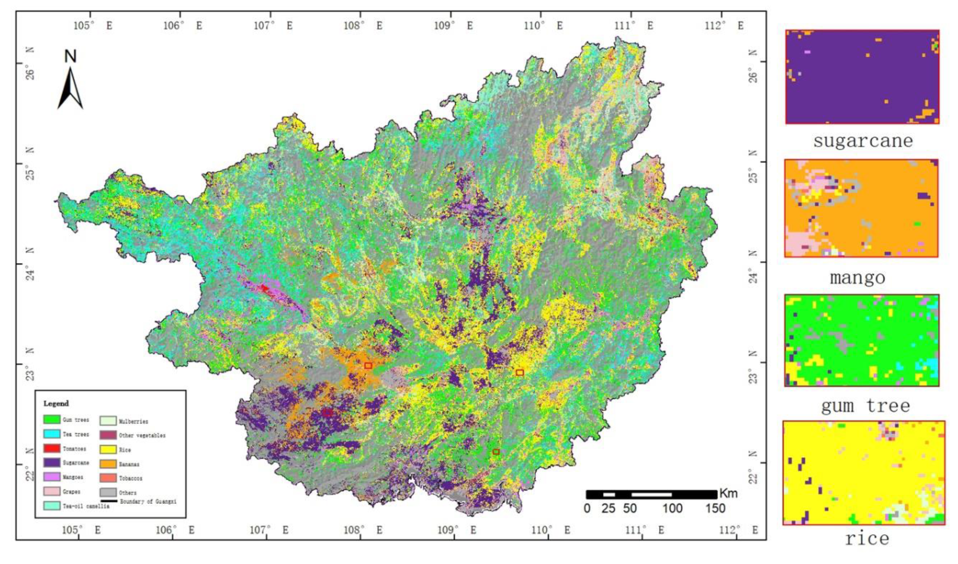
2. Study Area
3. Data
3.1. Field Data
3.2. Satellite MODIS Time Series
3.3. Digital Elevation Model (DEM)
4. Methods
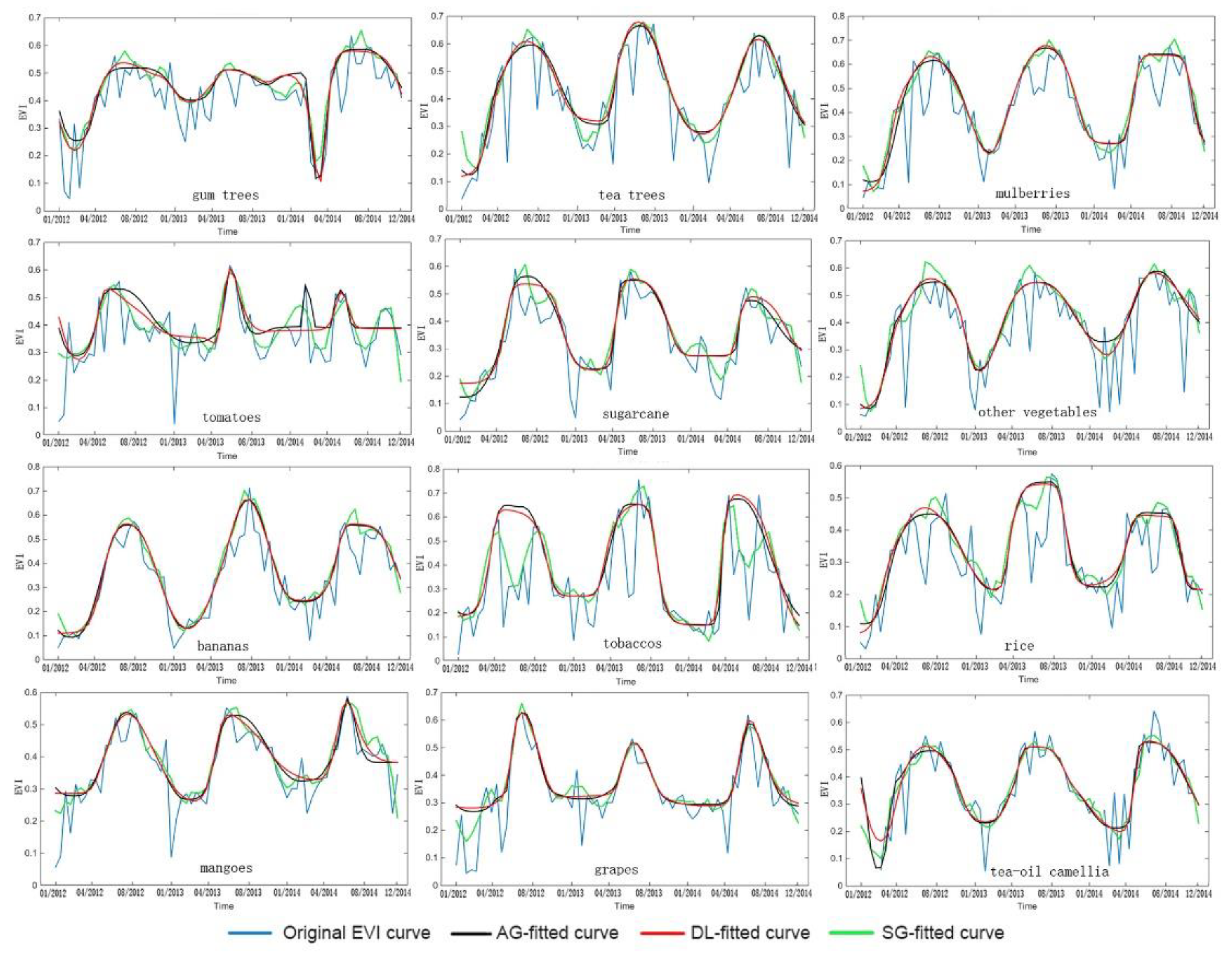
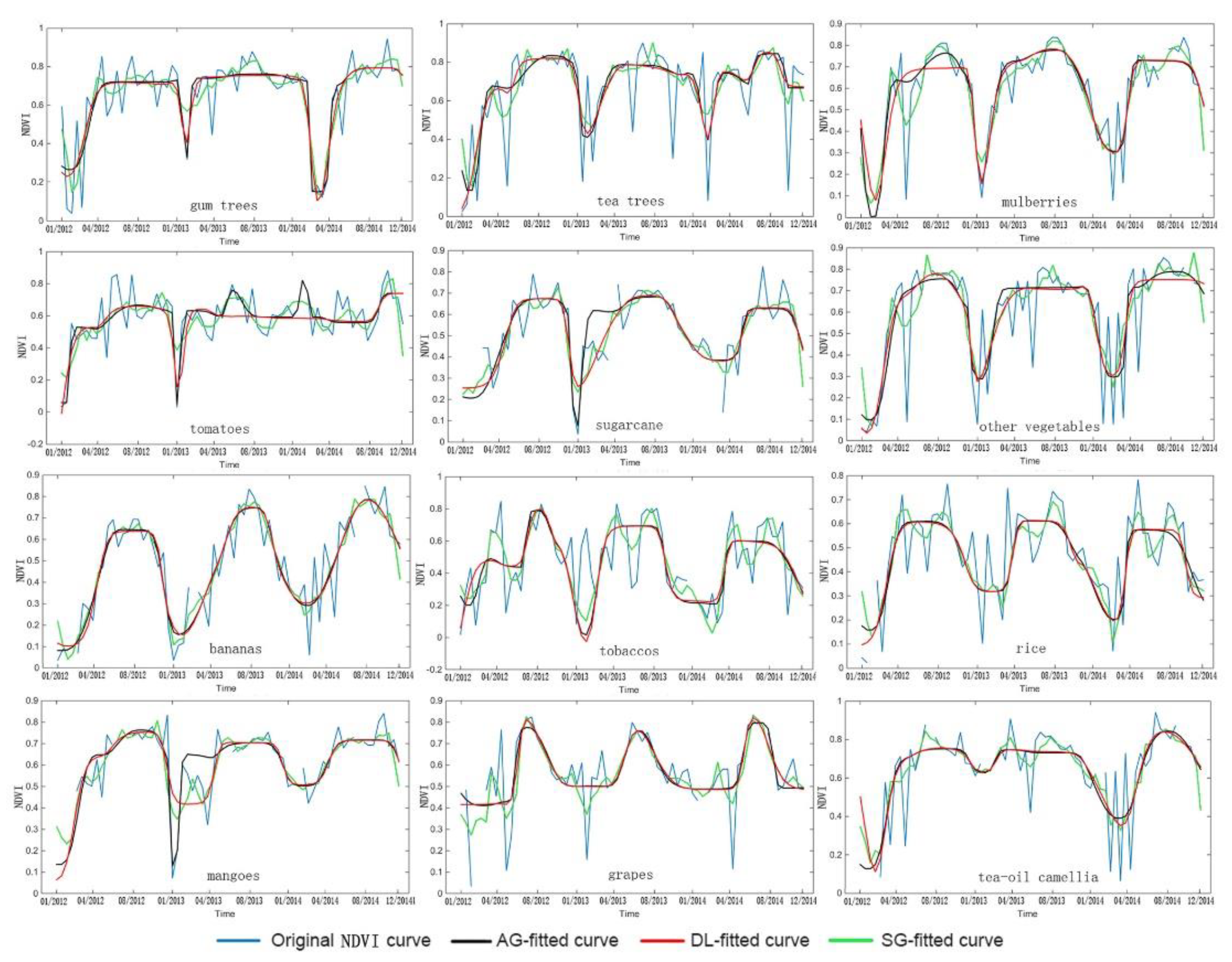
4.1. Derivation of Phenological Metrics
4.2. Random Forests Classification and Accuracy Assessment
5. Results and Discussion
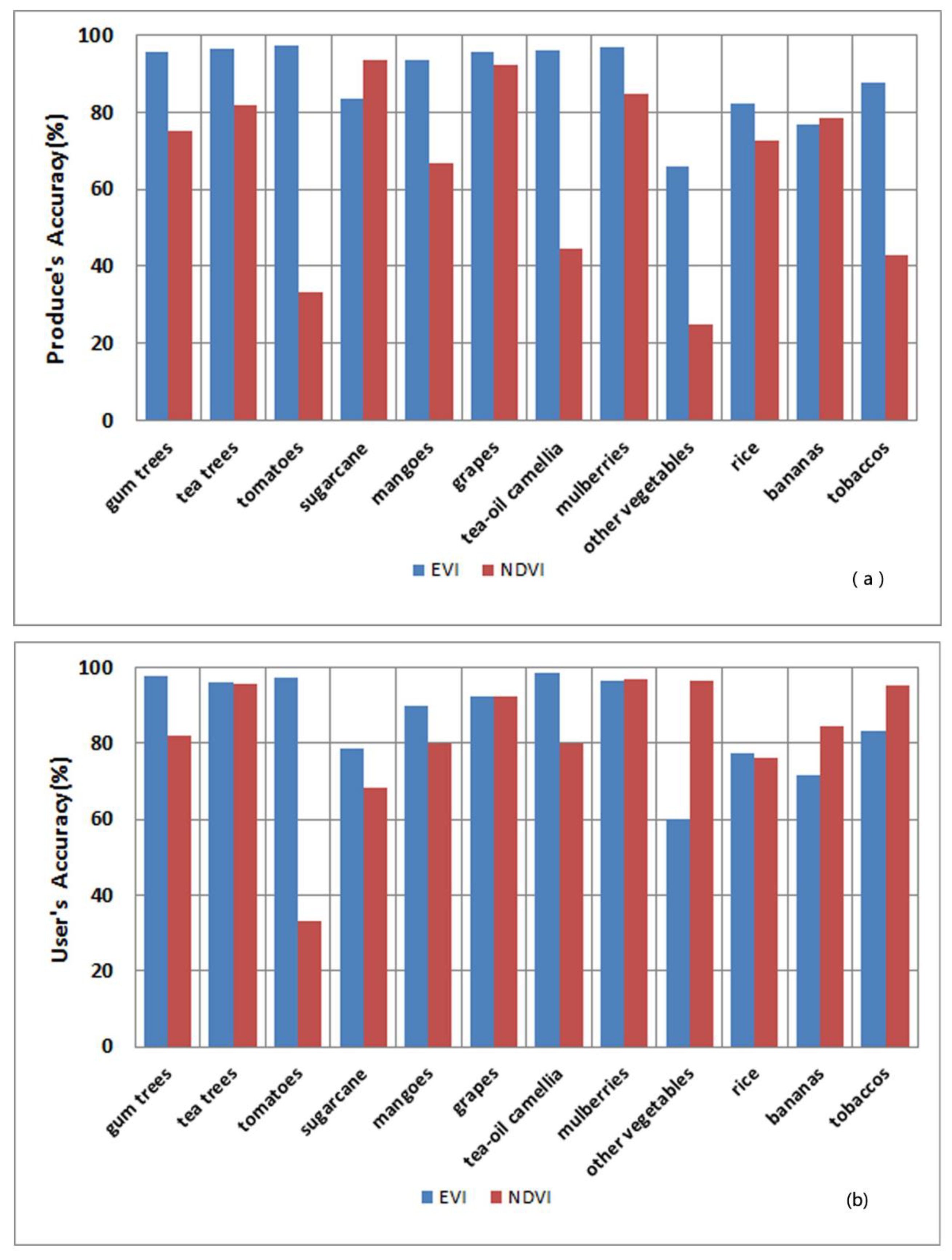
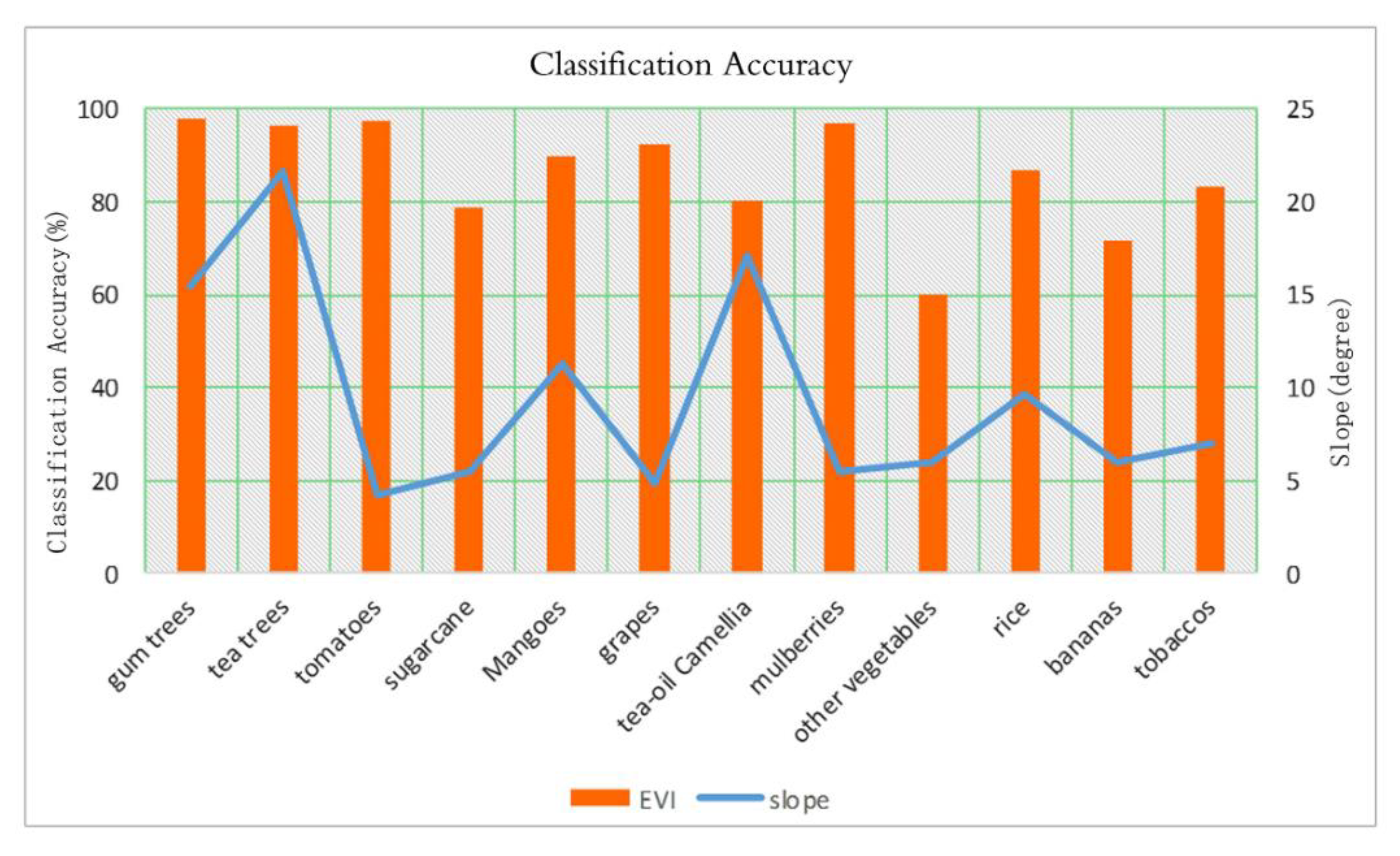
5.1. Classification Accuracy Assessment
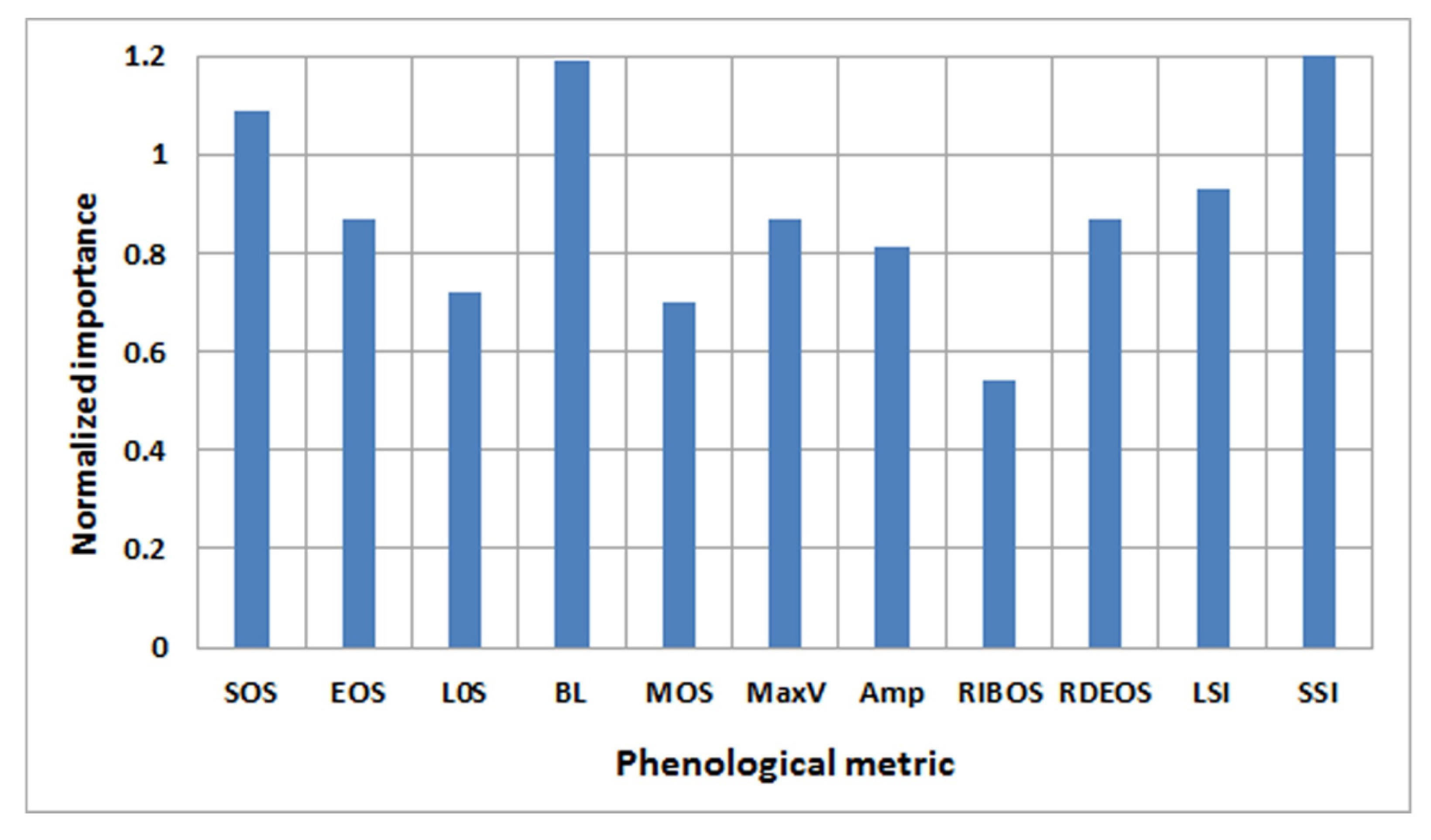
5.2. Importance of Phenological Metrics
5.3. Topographic Effects on Map Accuracy
6. Conclusions
Author Contributions
Funding
Conflicts of Interest
References
- Hutchinson, C.F. Uses of satellite data for famine early warning in sub-Saharan Africa. Int. J. Remote Sens. 1991, 12, 1405–1421. [Google Scholar] [CrossRef]
- Buyanovsky, G.A.; Wagner, G.H. Changing role of cultivated land in the global carbon cycle. Biol. Fertil. Soils 1998, 27, 242–245. [Google Scholar] [CrossRef]
- Lobell, D.B.; Asner, G.P.; Ortiz-Monasterio, J.I.; Benning, T.L. Remote sensing of regional crop production in the Yaqui Valley, Mexico: Estimates and uncertainties. Agric. Ecosyst. Environ. 2003, 94, 205–220. [Google Scholar] [CrossRef]
- Wright, S.J. Plant diversity in tropical forests: A review of mechanisms of species coexistence. Oecologia 2002, 130, 1–14. [Google Scholar] [CrossRef] [PubMed]
- Gibbs, H.K.; Ruesch, A.S.; Achard, F.; Clayton, M.K.; Holmgren, P. Tropical forests were the primary sources of new agricultural land in the 1980s and 1990s. Proc. Nat. Acad. Sci. USA 2010, 107, 16732–16737. [Google Scholar] [CrossRef] [PubMed]
- Wilson, K.D.P.; Reels, G.T. Odonata of Guangxi Zhuang autonomous Region, China, Part I: Zygoptera. Odonatologica 2003, 32, 237–279. [Google Scholar]
- Li, X.H.; Kong, L.Z.; Yang, J.F.; Yu, P.F. Development status and countermeasures of Guangxi fruit industry. Trop. Agric. Sci. 2016, 36, 79–85. [Google Scholar]
- Ning, X.; Kong, L.Z.; Shang, X.H.; Li, X.H.; Qin, Z.L. Guangxi vegetables industry development present situation and the countermeasure analysis. Trop. Agric. Sci. 2017, 37, 107–113. [Google Scholar]
- Bauer, M.E. The role of remote sensing in determining the distribution and yield of crops. Adv. Agron. 2015, 27, 271–304. [Google Scholar]
- Jewell, N. An evaluation of multi-date SPOT data for agriculture and land use mapping in the United Kingdom. Int. J. Remote Sens. 1989, 10, 939–951. [Google Scholar] [CrossRef]
- Moran, M.S.; Inoue, Y.; Barnes, E.M. Opportunities and limitations for image-based remote sensing in precision crop management. Remote Sens. Environ. 1997, 61, 319–346. [Google Scholar] [CrossRef]
- De Wit, A.J.W.; Clevers, J.G.P.W. Efficiency and accuracy of per-field classification for operational crop mapping. Int. J. Remote Sens. 2004, 25, 4091–4112. [Google Scholar] [CrossRef]
- Atzberger, C. Advances in Remote Sensing of Agriculture: Context Description, Existing Operational Monitoring Systems and Major Information Needs. Remote Sens. 2013, 5, 949–981. [Google Scholar] [CrossRef]
- Zhong, L.; Gong, P.; Biging, G.S. Efficient corn and soybean mapping with temporal extendability: A multi-year experiment using Landsat imagery. Remote Sens. Environ. 2014, 140, 1–13. [Google Scholar] [CrossRef]
- Pan, Y.; Li, L.; Zhang, J.; Liang, S.; Zhu, X.; Sulla-Menashec, D. Winter wheat area estimation from MODIS-EVI time series data using the Crop Proportion Phenology Index. Remote Sens. Environ. 2012, 119, 232–242. [Google Scholar] [CrossRef]
- Vieira, M.A.; Formaggio, A.R.; Rennó, C.D.; Atzberger, C.; Aguiar, D.A.; Mello, M.P. Object based image analysis and data mining applied to a remotely sensed Landsat time-series to map sugarcane over large areas. Remote Sens. Environ. 2012, 123, 553–562. [Google Scholar] [CrossRef]
- Zheng, B.; Myint, S.W.; Thenkabail, P.S.; Aggarwal, R.M. A support vector machine to identify irrigated crop types using time-series Landsat NDVI data. Int. J. Appl. Earth Obs. Geoinf. 2015, 34, 103–112. [Google Scholar] [CrossRef]
- Bargiel, D. A new method for crop classification combining time series of radar images and crop phenology information. Remote Sens. Environ. 2017, 198, 369–383. [Google Scholar] [CrossRef]
- Belgiu, M.; Csillik, O. Sentinel-2 cropland mapping using pixel-based and object-based time-weighted dynamic time warping analysis. Remote Sens. Environ. 2017, 204, 509–523. [Google Scholar] [CrossRef]
- Xiao, X.; Boles, S.; Frolking, S.; Li, C.; Babu, J.Y.; Salas, W.; Moore, B. Mapping paddy rice agriculture in South and Southeast Asia using multi-temporal MODIS images. Remote Sens. Environ. 2006, 100, 95–113. [Google Scholar] [CrossRef]
- Senf, C.; Pflugmacher, D.; Linden, S.V.D.; Hostert, P. Mapping rubber plantations and natural forests in Xishuangbanna (Southwest China) using multi-spectral phenological metrics from MODIS time series. Remote Sens. 2013, 5, 2795–2812. [Google Scholar] [CrossRef]
- Boschetti, M.; Busetto, L.; Manfron, G.; Laborte, A.; Asilo, S.; Pazhanivelan, S.; Nelson, A. PhenoRice: A method for automatic extraction of spatio-temporal information on rice crops using satellite data time series. Remote Sens. Environ. 2017, 194, 347–365. [Google Scholar] [CrossRef]
- Sianturi, R.; Jetten, V.G.; Sartohad, J. Mapping cropping patterns in irrigated rice fields in West Java: Towards mapping vulnerability to flooding using time-series MODIS imageries. Int. J. Appl. Earth Obs. Geoinf. 2017, 66, 1–13. [Google Scholar] [CrossRef]
- Gumma, M.; Pyla, K.; Thenkabail, P.; Reddi, V.; Naresh, G.; Mohammed, I.; Rafi, I. Crop Dominance Mapping with IRS-P6 and MODIS 250-m Time Series Data. Agriculture 2014, 4, 113–131. [Google Scholar] [CrossRef]
- Song, X.P.; Potapov, P.V.; Krylov, A.; King, L.A.; Bella, C.M.D.; Hudson, A.; Khan, A.; Adusei, B.; Stehman, S.V.; Hansen, M.C. National-scale soybean mapping and area estimation in the United States using medium resolution satellite imagery and field survey. Remote Sens. Environ. 2017, 190, 383–395. [Google Scholar] [CrossRef]
- Zhang, J.; Feng, L.; Yao, F. Improved maize cultivated area estimation over a large scale combining MODIS–EVI time series data and crop phenological information. ISPRS J. Photogramm. Remote Sens. 2014, 94, 102–113. [Google Scholar] [CrossRef]
- Skakun, S.; Franch, B.; Vermote, E.; Roger, J.; Becker-Reshef, I.; Justice, C.; Kussul, N. Early season large-area winter crop mapping using MODIS NDVI data, growing degree days information and a Gaussian mixture model. Remote Sens. Environ. 2017, 195, 244–258. [Google Scholar] [CrossRef]
- Wardlow, B.D.; Egbert, S.L. Large-area crop mapping using time-series MODIS 250m NDVI data: An assessment for the U.S. Central Great Plains. Remote Sens. Environ. 2008, 112, 1096–1116. [Google Scholar] [CrossRef]
- Wang, C.; Fan, Q.; Li, Q.; SooHoo, W.M.; Lu, L. Energy crop mapping with enhanced TM/MODIS time series in the BCAP agricultural lands. ISPRS J. Photogramm. Remote Sens. 2017, 124, 133–143. [Google Scholar] [CrossRef]
- Zhang, J.; Wu, S.H.; Liu, Y.H.; Yang, Q.Y.; Zhang, Y.H. The spatial simulation of agricultural production in Tibet under the influence of land use and topographic factors. Trans. Chin. Soc. Agric. Eng. 2007, 23, 59–65. [Google Scholar]
- Government of Guangxi. Available online: http://www.gov.cn/test/2013-04/16/content_2378978.htm (accessed on 29 April 2019).
- Jönsson, P.; Eklundh, L. TIMESAT—A program for analyzing time-series of satellite sensor data. Comput. Geosci. 2004, 30, 833–845. [Google Scholar]
- ASTER GDEM Validation Team. ASTER Global Digital Elevation Model Version 2—Summary of Validation Results. 2011. Available online: https://asterweb.jpl.nasa.gov/gdem.asp (accessed on 29 April 2019).
- Chen, G.; He, Y.; De Santis, A.; Li, G.; Cobb, R.; Meentemeyer, R.K. Assessing the impact of emerging forest disease on wildfire using Landsat and KOMPSAT-2 data. Remote Sens. Environ. 2017, 195, 218–229. [Google Scholar] [CrossRef]
- Eklundh, L.; Jönsson, P. Timesat 3.3 Software Manual; Lund and Malmö University: Lund, Sweden, 2017. [Google Scholar]
- Hird, J.N.; McDermid, G.J. Noise reduction of NDVI time series: An empirical comparison of selected techniques. Remote Sens. Environ. 2009, 113, 248–258. [Google Scholar] [CrossRef]
- Press, W.H. Numerical Recipes in Fortran; Cambridge University Press: Cambridge, UK, 1996; Volume 4, pp. 353–380. [Google Scholar]
- Breiman, L. Random Forests. Mach. Learn. 2001, 45, 5–32. [Google Scholar] [CrossRef]
- Liaw, A.; Wiener, M. Classification and Regression by Random Forest. R News 2002, 2, 18–22. [Google Scholar]
- Hultquist, C.; Chen, G.; Zhao, K. A Comparison of Gaussian Process Regression, Random Forests and Support Vector Regression for Burn Severity Assessment in Diseased Forests. Remote Sens. Lett. 2014, 5, 723–732. [Google Scholar] [CrossRef]
- Van der Linden, S.; Rabe, A.; Held, M.; Jakimow, B.; Leitão, P.J.; Okujeni, A.; Schwieder, M.; Suess, S.; Hostert, P. The EnMAP-Box—A Toolbox and Application Programming Interface for EnMAP Data Processing. Remote Sens. 2015, 7, 11249–11266. [Google Scholar] [CrossRef]
- Huete, A.; Didan, K.; Miura, T.; Rodriguez, E.P.; Gao, X.; Ferreira, L.D. Overview of the radiometric and biophysical performance of the MODIS vegetation indices. Remote Sens. Environ. 2002, 83, 195–213. [Google Scholar] [CrossRef]


| Phenological Metric | Explanation |
|---|---|
| Time for the start of the season (SOS) | Time for which the value (EVI/NDVI) has increased to a user-defined level (i.e., 10% of the distance between the left minimum level and the maximum). |
| Time for the end of the season (EOS) | Time for which the right edge has decreased to a user-defined level measured from the right minimum level (i.e., the 10% of the distance between the right minimum level and the maximum). |
| Length of the season (LOS) | Time from the start to the end of the season. |
| Base level (BL) | Given as the average of the left and right minimum values. |
| Time for the mid of the season (MOS) | Computed as the mean value of the times for which, respectively, the left edge has increased to the 80% level and the right edge has decreased to the 80% level. |
| Largest data value for the fitted function during the season (MaxV) | It may occur at a different time compared with MOS. |
| Seasonal amplitude (Amp) | Difference between the maximum value and the base level. |
| Rate of increase at the beginning of the season (RIBOS) | Calculated as the ratio of the difference between the left 20% and 80% levels and the corresponding time difference. |
| Rate of decrease at the end of the season (RDEOS) | Calculated as the absolute value of the ratio of the difference between the right 20% and 80% levels and the corresponding time difference. The rate of decrease is thus given as a positive quantity. |
| Large seasonal integral (LSI) | Integral of the function describing the season from the season start to the season end. |
| Small seasonal integral (SSI) | Integral of the difference between the function describing the season and the base level from season start to season end. |
| Land Surface Type | Cultivation Area (km2) |
|---|---|
| Gum trees | 20,259.9 |
| Tea trees | 3189.4 |
| Tomatoes | 410.8 |
| Sugarcane | 19,456.9 |
| Mangoes | 12,773.4 |
| Grapes | 7551.8 |
| Tea-oil camellia | 9995.8 |
| Mulberries | 1750.3 |
| Other vegetables | 3353.0 |
| Rice | 21,560.2 |
| Bananas | 12,706.0 |
| Tobaccos | 410.8 |
© 2019 by the authors. Licensee MDPI, Basel, Switzerland. This article is an open access article distributed under the terms and conditions of the Creative Commons Attribution (CC BY) license (http://creativecommons.org/licenses/by/4.0/).
Share and Cite
Wei, Y.; Tong, X.; Chen, G.; Liu, D.; Han, Z. Remote Detection of Large-Area Crop Types: The Role of Plant Phenology and Topography. Agriculture 2019, 9, 150. https://doi.org/10.3390/agriculture9070150
Wei Y, Tong X, Chen G, Liu D, Han Z. Remote Detection of Large-Area Crop Types: The Role of Plant Phenology and Topography. Agriculture. 2019; 9(7):150. https://doi.org/10.3390/agriculture9070150
Chicago/Turabian StyleWei, Yanfei, Xinhua Tong, Gang Chen, Deqiang Liu, and Zhenfeng Han. 2019. "Remote Detection of Large-Area Crop Types: The Role of Plant Phenology and Topography" Agriculture 9, no. 7: 150. https://doi.org/10.3390/agriculture9070150
APA StyleWei, Y., Tong, X., Chen, G., Liu, D., & Han, Z. (2019). Remote Detection of Large-Area Crop Types: The Role of Plant Phenology and Topography. Agriculture, 9(7), 150. https://doi.org/10.3390/agriculture9070150