Abstract
Over recent decades several European and global occurrences have had an impact on the European Union’s economic sectors, and subsequently on farms. In fact, the various Common Agricultural Policy (CAP) reforms, namely those since 1992, and the global financial and economic crises, specifically after 2008, seem to have had several effects on the dynamics of the entire European Union agricultural sector and on the performance of farms. However, there is doubt as to whether these events were enough to promote structural breaks in European Union farms. In this way, the main objective of this study is to analyse both the known and unknown structural breaks in European farms, between 1989 and 2016. To this purpose, data from the Farm Accountancy Data Network (FADN) from the twelve former member-states (the countries with the longer time series) and methodologies based on the Chow test and on the Quandt likelihood ratio (QLR) were considered. The results show that the structural breaks are different across the several twelve former European Union countries and among the several variables considered. In any case, the financial and economic crises, as well as changes in the European Union’s methodologies relative to statistical information, seem to have had a greater impact on the European farms than the several CAP reforms (with the exception of the reform of 1992 the trade liberalization). However, the several consequences of all these European and world events on European farms seem to be delayed for some years.
Keywords:
structural breaks; European Union farms; farm accountancy data network; Chow and Quandt likelihood ratio tests; time series regressions Jel Classification:
C22; O13; Q12
1. Introduction
This investigation aims to answer the following question: are the different CAP (Common Agricultural Policy) reforms, the world financial crisis and other European (German reunification) and international events relevant to promoting structural breaks within the European Union agricultural sector?
In a relatively highly regulated sector and with a great diversity of contexts or realities, such as European Union agriculture, it is normal to expect frequent changes in the instruments derived from agricultural policies. In fact, the Common Agricultural Policy has suffered several changes over recent decades, as a consequence of many factors, such as the natural evolution of the farms and the successive European Union enlargements [1].
Parallel to this evolution of the European agricultural policies, other world events occurred, such as the world financial and economic crisis, that eventually, also, impacted upon the dynamics and the performance of the farming sector in the European Union member-states. In fact, the global crisis of 2008 had an immediate impact on the socioeconomic indicators in many countries and was delayed in other countries.
The question here, is if these events (namely CAP reforms and the global crisis) promoted structural breaks in the several indicators of European Union farms. The CAP created at the beginning of the European Economic Community (EEC), at the end of the fifties, was designed with two main policies. First with one policy directed at the markets and farmers’ income and later with the other directed at agricultural and rural investments and structures [1]. The market and farmers’ income policy has undergone several reforms, namely in 1992, 1999, 2003, 2007 and 2013. The structural agricultural policy often appears more recently within the community support frameworks for all sectors and with reforms after periods of around seven years. All of these policy instruments had objectives for the agricultural sector and their assessment is a determinant to support the design of new policies. On the other hand, the European (German reunification) and international events had consequences on the farms’ structures, and so it is important to assess their dimensions. This could be important to better understand the behaviour of farms in reaction to different impacts, as insights for the several stakeholders, namely for the policymakers.
In this framework it seems important to analyse the structural breaks over recent decades in European Union farms. For this, time series data for the period 1989–2016 from the Farm Accountancy Data Network [2] was considered. The statistical information available in this database, for each country, is relative to a “representative farm”, obtained through a methodology described by the FADN. In any case, as a small explanation, it is worth highlighting that this database represents about 90% of the European Union’s utilized agricultural area and total farming production and is considered to analyse European Union farms and the impact of the CAP. Considering the importance of these data for the agricultural policies analyses and design, they should be as accurate as is possible. For this the European Commission and the member-state institutions must guarantee this capacity. In terms of methodology adopted by the FADN it is crucial to note the following three important aspects: field of survey; sample selection; and weighting. The field of observation is constituted by commercial farms. A commercial farm may be defined in a simple way such as an agricultural unit that produces enough to support the farmer and his/her family, however, in general, this definition follows rules and legislation from the European Union and member-states. For the sample selection, the farms heterogeneity was considered through a stratification approach and the main types of farming (typology) were taken into account, whose process of identification is based on the standard output (average farming output) or standard gross margin (average farming output less certain specific costs). Finally, a weighting approach was considered to obtain the European Union FADN results. This microeconomic information has the advantage of allowing for an understanding of the specific characteristics of the farms in each of the member-states over the period taken into account. Methodologies were also considered so as to test the structural breaks, such as the Chow [3] and Quandt likelihood ratio [4] tests. Another question analysed here is the impact of joining together the two FADN time series. In fact, considering different assumptions, the FADN has two time series, one for the period 1989–2009 and the other for the period 2004–2016 (annually actualized with more recent data), which frequently brings about difficulties when there is an intention to use longer time series and more recent statistical information. In this way, the data for the former twelve member-states and the whole European Union were analysed through joining the two periods in 2010 (maintaining the longer time series from the first period), and for the whole European Union by putting the data from the periods together in 2004. The junction of the two periods for the whole European Union in 2004 and 2010 was one more approach towards understanding the impact of the change of methodology implemented by the FADN in the evolution of the time series in the two periods. The main changes implemented by the FADN in 2010 were related to the measurement of the farms’ economic size (until 2009 based on the standard gross margin and since 2010 based on the standard output).
Considering the organization of the database and contributions from, for example, Martinho [5], the following variables were analysed: labour input (hours); total utilised agricultural area (ha); total livestock units (units); total output (euros); total output crops (euros); total output livestock (euros); total inputs (euros); subsidies on investments (euros); total assets (euros); and total subsidies-excluding investments (euros). The CAP reforms since 1992 intend, namely, to reduce the excesses of production and promote farm dimension. In this way these variables seem adjusted to properly assess the impacts from the CAP reforms, as well as, from other European and international events. The subsidies are, also, relevant variables, since the several CAP instruments are supported by subsidies (to the investment and to the farmers’ income) that often change with the CAP reforms.
The remaining parts of this study are relative to the literature survey, data analysis, structural breaks test and a regression based on the Cobb and Douglas [6] model.
2. Insights from Literature
The agricultural sector is, indeed, vulnerable to several shocks, namely those from farming policies, trade liberalization and financial and economic crises. In a global perspective, to highlight the importance of these shocks on the agricultural evolution, it is pertinent to refer to, for example, the trade liberalization and the world financial crisis which were identified as causes of structural breaks in Chinese agri-food exports [7] and the Great Depression in the twenties was identified as having heavily influenced US agricultural productivity [8]. The financial crisis also had its influence upon the Indian commodity markets, including the agricultural commodity chains [9]. On the other hand, agricultural policies and the manufacturing dynamics had their influences over the seventies/eighties in Chinese agricultural productivity [10]. However, the question is what are the factors and how do they impact upon the several indicators for agriculture around the world and, specifically, in the European Union countries?
To show the flexibility of the methodology, namely that which was used to test for structural breaks in the time series related to the agricultural sector, depending on the objective of each study and the database considered, the more diverse indicators were considered, from productivity [11], to others, such as the temperature over agro climatic areas [12].
On the other hand, the structural breaks may be analysed through different approaches, some, for example, considering each variable individually and other investigating relationships between several variables. For example, Beckman and Schimmelpfennig [13] analysed the relationships between farm income, the range of prices and the technological changes, allowing for structural breaks. In turn, Buberkoku [14] considered structural breaks when analysing the relationships between the US dollar’s exchange and commodity prices. Indeed, the several dimensions in the contexts of the exchange rates have their implications, for example, in the evolution of the agricultural sector [15]. Gokmenoglu and Taspinar [16] allowing for structural breaks when investigating the environmental frameworks involving the agricultural sector. Lee and Hsu [17] considered the relationships between public investment in the agricultural sector and farming productivity. In other cases, the relationships between financial development and energy consumption were considered, taking into account questions related to the agricultural sector, for example [18]. Considering the specificities of all contexts related to the agricultural sector, it is prudent in allowing for structural breaks in the several analyses involving time series data [19].
Specifically, for the European Union, it is worth highlighting that the literature shows that the internal evolution and the international events have their implications on the agricultural sector and food industry [20]. Amid the international events having impacts on the European economic sectors, the 2008 financial/economic crisis appears as one of the most relevant occurrences [21]. Inside the European Union, the CAP reforms had determinant consequences on the agricultural sector, as well as upon the whole economy [22]. Indeed, the CAP reforms, German reunification, the World Trade Organization (WTO) negotiations and the financial crisis of 2008 were the more relevant events posing implications on the European Union agricultural sector.
The analyses about the existence of structural breaks can be performed to try to identify the years within the time series where there were changes (unknown breaks) or to confirm, sometimes in models involving several variables, structural breaks which have been previously identified [23].
3. Data Analysis
Figure 1 illustrates the evolution, over the period considered, for the variables considered in this study and referred to before in Section 1. Note that the evolution of the data for the entire European Union, resulting from conjoining the two periods (1989–2009 and 2004–2016) in 2004 and 2010, does not present relevant differences.
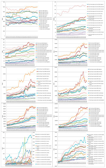
Figure 1.
Evolution of several farm accountancy variables over the European Union countries (1989–2016).
Relative to the labour, this figure shows that the Netherlands, the United Kingdom, Germany and Belgium are the countries where the “representative farm” has more labour input (around 6000 hours in the Netherlands and around 5000 hours in the United Kingdom, Germany and Belgium, in 2016). With the exception for some European Union countries (for example, the increasing trend after 2000 for the Netherlands and after 1994 for Germany and the decreasing trend for France after 2001), in general the evolution of labour since 1989 to 2016 does not display any trend (almost appears as white noise).
In another way, the agricultural area utilized seems to present an increasing trend over the period considered for the great part of these countries. It is interesting to highlight, for example, as verified for that with the labour, there is a change in the evolution after 1994 for Germany. On the other hand, the “representative farm” has more agricultural area utilized, for a great part of this period, in the United Kingdom, Denmark, Germany, France and Luxembourg and less area in Greece, Italy and Portugal.
For the total livestock, there was, also, an increasing trend over the period for the majority of countries, with an exception maybe, for example, in Ireland and the whole European Union. It is worth stressing, for example, the relevant changes in the evolution of the total livestock in Denmark after 1991 (strong increase) and after 2011 (heavy decrease). Denmark, the Netherlands, the United Kingdom, Belgium, Luxembourg and Germany are the countries where there are more livestock units per farm.
The increasing trend, in general, is verified for the remaining variables related with the output, input, assets and subsidies, with the exception of the subsidies on investments where the evolution for the several countries is more difficult to read.
In any case observe that the Netherlands and Denmark are the countries with more total output, namely at the end of the period. On the other hand, it seems that there was a decreasing break in a significant number of countries around 2008/2009 and 2012/2013/2014 relative to this variable. In addition to the specificities relative to the specialization of some European Union countries in more crops or more livestock, the context described for the total output is similar to that verified for the crops output, livestock output and total input.
These breaks are not so clear for the total assets and subsidies, however it seems there is a decreasing trend at the end of the period, namely for the total assets and total subsidies-excluding investments.
4. Finding Unknown Structural Breaks
In this section, to search for unknown structural breaks, the Quandt likelihood ratio (QLR) statistics (with a critical value of 3.66 at 5%) will be considered, following the procedures proposed by Torres-Reyna [24], Stock and Watson [25] and Stata [26]. With the QLR statistics the intention is to find the main break over a period of time, considering a specific critical value [27].
Figure 2, concerning the breaks for labour, reveals that 2011 seems to have been the year with the greater structural break in a significant amount of European Union countries, eventually as a delayed consequence of the global financial crisis of 2008 and maybe as an implication from changes in the statistical methodologies adopted by the European Union. In Denmark the greater structural break seems to have occurred before 2011 (2005 or 2009); Germany in 1995 (as observed in Section 3 regarding the data analysis), France in 2009, Italy in 2012, Luxembourg in 1996, Portugal in 1997, the United Kingdom in 2009 and the European Union-2010 (conjoining of the two time series available in the FADN, in 2010) in 1997. It seems that the CAP reform of 1992 and the WTO changes (after the Uruguay Round of 1986–1994) had a delayed effect in several countries, as an almost immediate impact from the global financial crisis in some countries and delayed in others and, as well, had implications on the changes in the methodologies implemented by the European Union to collect and organize statistical information.
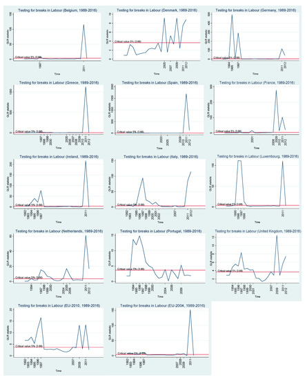
Figure 2.
Testing for breaks in labour (hours) over the European Union countries (1989–2016).
Relative to the utilized agricultural area, Figure 3 shows that greater breaks, for the European Union countries, occurred towards the end of the nineties, around 2009 and around 2011, confirming the delayed impact from the CAP and WTO reforms and the implications from the global financial crisis and statistical methodological changes.
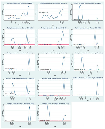
Figure 3.
Testing for breaks in utilized agricultural area (hectares) over the European Union countries (1989–2016).
Figure 4, relative to the livestock units, confirms the context previously described for Figure 2 and Figure 3 (for labour and utilized agricultural area, respectively). In any case, it is worth stressing that in this phase, some patterns were verified for each European Union country. For example, Belgium had their greater structural breaks around 2009 and 2011, showing that it was more influenced, on farming labour, area and livestock, by the global financial crisis and statistical methodological changes. The same happened for Denmark (with the exception of a great structural break verified in 2005 in labour), for Greece, Spain (in this case mostly around 2011), France (more around 2009), Ireland (more around 2011), Italy (around 2011, with the exception of livestock, where the break occurred around 1996), the Netherlands and the United Kingdom. Germany is clearly a case where the greater structural breaks, for labour, area and livestock, occurred at the end of the nineties, showing signs that this country benefitted from the German reunification, CAP reforms and WTO negotiations from the nineties. Of course, there were other events, but these were referred to by the literature as the most relevant in this period. Something similar was verified for Luxembourg (with some differences in trends, for example, for labour, relative to Germany, as shown in Figure 1). Portugal presents stronger structural breaks at the end of the nineties for labour and livestock and around 2011 for the utilized agricultural area. Portugal had a decreasing tendency in farming labour over 1989–2016 (Figure 1). The whole European Union-2010 countries show breaks at the end of the nineties for farming labour and around 2011 and 2008 for the area and livestock, respectively. The EU-2004 presents breaks around 2011 (labour), in the nineties (area) and around 2006 (livestock).
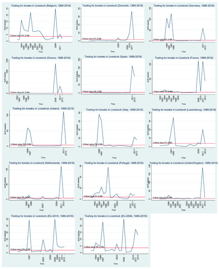
Figure 4.
Testing for breaks in livestock units over the European Union countries (1989–2016).
Except for Belgium, Germany, Ireland, Luxembourg and Portugal (with breaks in the late nineties), the majority of the European Union countries presented structural breaks for the total farming output around 2009 and 2011 (Figure 5), as verified in the data analysis in Section 3. Figure 6, for the crops output, reveals that the majority of the countries presented structural breaks around 2011, with the exception of Germany, the Netherlands and Portugal with stronger breaks in the nineties.
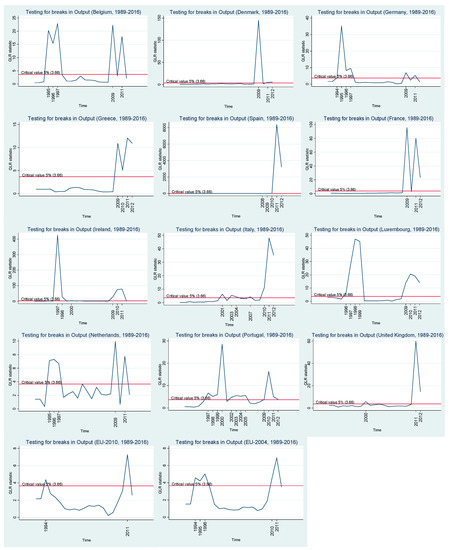
Figure 5.
Testing for breaks in total output (euros) over the European Union countries (1989–2016).
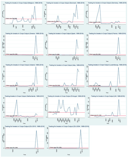
Figure 6.
Testing for breaks in crops output (euros) over the European Union countries (1989–2016).
The structural breaks, for the livestock output (Figure 7), are around 2009, and 2011, with the exception of Germany, the United Kingdom and the EU-2004 (with breaks in the nineties). The EU-2010 does not present any structural breaks, considering that all values for the QLR test are below the critical value at 5%.
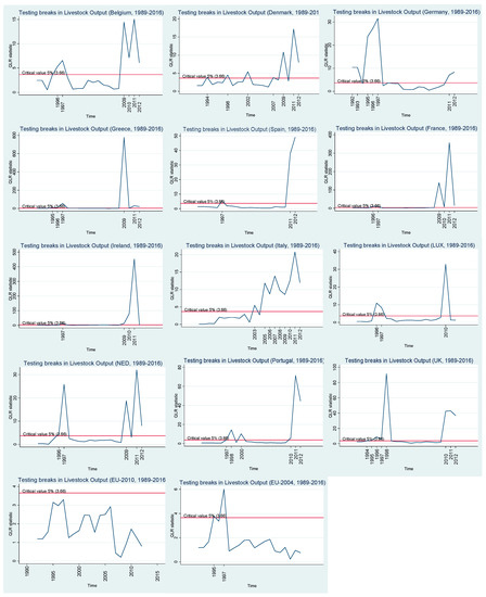
Figure 7.
Testing for breaks in livestock output (euros) over the European Union countries (1989–2016).
Figure 8 shows that the structural breaks for the total inputs are mainly around 2009 and 2011, with the only exception being Germany. For the total assets (Figure 9), in addition to the usual breaks around 2009 and 2011, there are structural changes at the end of the nineties for Germany, the Netherlands, Portugal, EU-2010 and EU-2004. Denmark shows, again, a strong structural break in 2005.
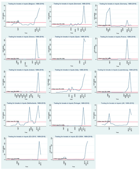
Figure 8.
Testing for breaks in total inputs (euros) over the European Union countries (1989–2016).
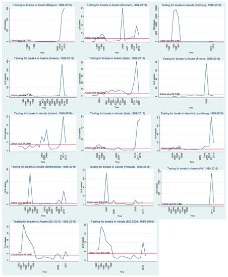
Figure 9.
Testing for breaks in total assets (euros) over the European Union countries (1989–2016).
The subsidies on investments (Figure 10) clearly present structural breaks around 2011, including Germany (with the exception of Denmark). Relative to the subsidies-excluding those on investments, again, the majority of the structural breaks occurred around 2011, with an exception for Germany, rather than benefitting from the reforms verified at the end of the nineties (Figure 11).
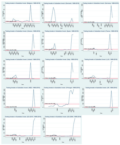
Figure 10.
Testing for breaks in subsidies on investments (euros) over the European Union countries (1989–2016).
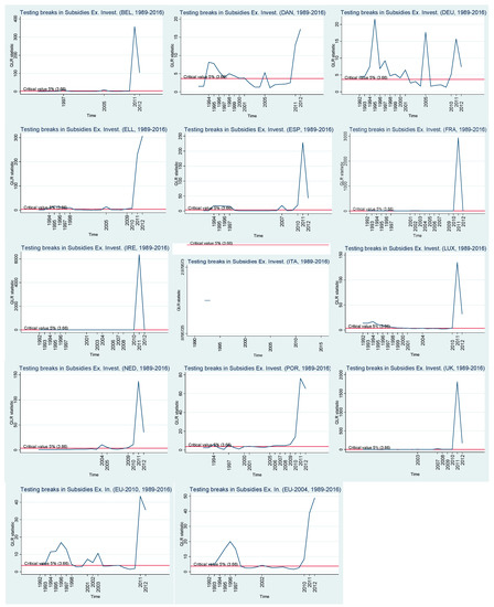
Figure 11.
Testing for breaks in total subsidies—excluding on investments (euros) over the European Union countries (1989—2016).
5. Results from Time Series Regressions with Known Breaks
Table 1 shows the results obtained through Newey-West standard error methodologies, based on the Cobb-Douglas model and allowing for structural breaks on the relationship, following the procedures proposed by Torres-Reyna [24] and Stata [26]. To allow for structural breaks, a dummy variable was found considering the results obtained in the previous section and the Chow test after several annual simulations (the majority of the breaks found for the model do not match those breaks found for the variables present in the relationship individually, with an exception, for example, for France).

Table 1.
Results for time series estimations with Newey-West standard errors, based on the Cobb-Douglas model (Output logarithm as dependent variable), over 1989–2016.
The Durbin’s and Breusch-Godfrey LM tests for autocorrelation reveal that there was time autocorrelation in the majority of the countries (corrected with the estimation methodologies considered), except for Greece and Luxembourg. On the other hand, the VIF for the multicollinearity (with or without the dummy variable) shows problems (5 was considered as an acceptable limit) in Denmark, Germany, Ireland and the Netherlands. As a result of this, in these cases, another regression was carried out with the labour logarithm in first difference (the labour seemed to have the variables that caused more problems in those countries).
The Chow test demonstrates that the relationship considered reveals structural breaks around the beginning of the period (1989–2016) in Belgium, Denmark, Germany, Spain and the whole of the European Union (2004 and 2010). In turn, the structural break of this model occurred around 2009 for Greece, France and Ireland, around 2001 for Italy, around 2005 for Luxembourg and the Netherlands and around 2000 for Portugal and the United Kingdom. The nineties and the year of 2009 seem to be the greater milestones for structural breaks in the relationship between farming output, labour and the assets (a proxy for capital). These dummy variables had a negative impact, on the total farming output, in Belgium and across the European Union and positive effects in the remaining countries (with an exception for Denmark, Germany and Greece, where the coefficients do not present statistical significance).
Farming labour improves the total farming output in Greece, Spain, France (with the lower coefficient) and Luxembourg and reduces the output, for example, in Portugal. The total assets clearly improve the farming output in all European Union countries, with greater values, for example, in Germany and Portugal and the lower values, for instance, in Ireland and Italy.
6. Conclusions
The main objective of this study was to analyse the structural breaks, over the period 1989–2016, for the twelve former European Union countries and for all European Union countries (considered together). For this purpose, statistical information from the Farm Accountancy Data Network and statistical methodologies, namely the Chow and QLR tests, were considered in order to find and analyse structural breaks, over the time series used. Another aim was to investigate the effects of joining together the two time series available in the FADN (1989–2009 and 2004–2016) in 2004 or in 2010. In fact, the FADN presents two different time series (the series 2004–2016 is annually updated), due to changes in the statistical methodology adopted, which brings about difficulties when attempting to use a longer and up to date series.
In this analysis the following farming variables were considered: labour input (hours); total utilised agricultural area (ha); total livestock units (units); total output (euros); total output crops (euros); total output livestock (euros); total input (euros); subsidies on investments (euros); total assets (euros); total subsidies-excluding investments (euros).
The results from the QLR test (for unknown breaks in the variables considered individually) clearly show that the mid to late nineties and the years around 2009 and 2011 is when there were more structural breaks. This shows that the CAP and WTO reforms in the middle of the nineties and the financial global crisis of 2008 had structural impacts on European Union farms, however with years of delay in some cases. Indeed, the great CAP reform of 1992 changed the paradigm of the European agricultural policies with the partial decoupling of income support. Financial support was partially decoupled from the levels of production to, in turn, be paid in relation to the farm’s dimension through direct aid to income. The idea behind this was to reduce the production in Europe (to avoid excess in production), reduce the environmental problems, reduce the financial expense and consider pressures from the World Trade Organization. After 1992 in Europe the paradigm has been to promote more rural development rather than agricultural growth. This framework had its implications on the dynamics of the farming sector across the European countries. In any case, Germany is clearly a case where structural breaks occurred as a consequence of the European and other world events occurring in the nineties, and it would appear that the farms benefitted from them. On the other hand, with the other CAP reforms verified in 2000, 2003 and later, it would seem that their impact upon European farms was less significant. The CAP reform of 2003 changed, again, the pattern of the CAP with the full decoupling and the introduction of the single payment scheme. The aim here was to continue supporting the farmers’ income through a single payment (considering the historical direct aid support) without the obligation of producing the agricultural activities under financial support (as it had previously been after 1992), allowing the farmers to decide on and produce the agricultural activities they considered as being more adjusted to their resources and objectives (of course with some obligations). This framework seems to have had less impact on the European farming dynamics than that verified by the CAP reform of 1992.
The results obtained with the regressions, based on the a Cobb-Douglas linear model, between the total farming output, the labour and the total assets (proxy for the capital) reveal that with the variables put together, the structural breaks found do not match, in the majority of cases, those found with the variables (present in the relationship) considered individually (with the exception of France, where the year of 2009 is clearly a break). The impact of these structural breaks present in the model depends on the country considered. On the other hand, the total farming assets are fundamental to improving the total output in European Union countries.
Finally, with regard to the question posed at the beginning of this study (first few lines of introduction) section, the findings of this research show that the CAP and WTO reforms of the nineties (as well as the German reunification) and the financial crisis of 2008 did indeed cause determinant structural breaks in the European Union agricultural sector.
Funding
This work is supported by national funds, through the FCT–Portuguese Foundation for Science and Technology under the project UID/SOC/04011/2019.
Conflicts of Interest
The author declares no conflict of interest.
References
- Martinho, V.J.P.D. Insights from over 30 years of common agricultural policy in Portugal. Outlook Agric. 2017, 46, 223–229. [Google Scholar] [CrossRef]
- FADN. Agriculture—FADN: F. A. D. N.—Homepage [WWW Document]. 2018. Available online: http://ec.europa.eu/agriculture/rica/ (accessed on 14 September 2018).
- Chow, G.C. Tests of Equality between Sets of Coefficients in Two Linear Regressions. Econometrica 1960, 28, 591–605. [Google Scholar] [CrossRef]
- Quandt, R.E. Tests of the Hypothesis that a Linear Regression System Obeys Two Separate Regimes. J. Am. Stat. Assoc. 1960, 55, 324–330. [Google Scholar] [CrossRef]
- Martinho, V.J.P.D. Characterization of agricultural systems in the European Union regions: A farm dimension- competitiveness-technology index as base. Reg. Sci. Inq. 2018, 10, 135–152. [Google Scholar]
- Cobb, C.W.; Douglas, P.H. A Theory of Production. Am. Econ. Assoc. 1928, 18, 139–165. [Google Scholar]
- Guo, Z.; Feng, Y.; Gries, T. Changes of China’s agri-food exports to Germany caused by its accession to WTO and the 2008 financial crisis. Chin. Agric. Econ. Rev. 2015, 7, 262–279. [Google Scholar] [CrossRef]
- Oehmke, J.F.; Schimmelpfennig, D.E. Quantifying Structural Change in U.S. Agriculture: The Case of Research and Productivity. J. Product. Anal. 2004, 21, 297–315. [Google Scholar] [CrossRef]
- Shalini, V.; Prasanna, K. Impact of the financial crisis on Indian commodity markets: Structural breaks and volatility dynamics. Energy Econ. 2016, 53, 40–57. [Google Scholar] [CrossRef]
- Nin-Pratt, A.; Yu, B.; Fan, S. Comparisons of agricultural productivity growth in China and India. J. Product. Anal. 2010, 33, 209–223. [Google Scholar] [CrossRef]
- Ball, E.; Schimmelpfennig, D.; Wang, S.L. Is U.S. Agricultural Productivity Growth Slowing? Appl. Econ. Perspect. Policy 2013, 35, 435–450. [Google Scholar] [CrossRef]
- Paul, R.K.; Birthal, P.S.; Khokhar, A. Structural Breaks in Mean Temperature over Agroclimatic Zones in India. Sci. World J. 2014, 2014, 1–9. [Google Scholar] [CrossRef] [PubMed]
- Beckman, J.; Schimmelpfennig, D. Determinants of farm income. Agric. Finance Rev. 2015, 75, 385–402. [Google Scholar] [CrossRef]
- Buberkoku, O. The Impact of the US Dollar’s Movements on Commodity Prices. Ege Acad. Rev. 2017, 17, 323–336. [Google Scholar] [CrossRef]
- Erdem, E.; Nazlioglu, S.; Erdem, C. Exchange rate uncertainty and agricultural trade: panel cointegration analysis for Turkey. Agric. Econ. 2010, 41, 537–543. [Google Scholar] [CrossRef]
- Gökmenoglu, K.K.; Taspinar, N. Testing the agriculture-induced EKC hypothesis: The case of Pakistan. Environ. Sci. Pollut. Res. 2018, 25, 22829–22841. [Google Scholar] [CrossRef] [PubMed]
- Lee, C.C.; Hsu, Y.C. Endogenous structural breaks, public investment in agriculture and agricultural land productivity in Taiwan. Appl. Econ. 2009, 41, 87–103. [Google Scholar] [CrossRef]
- Shahbaz, M.; Islam, F.; Butt, M.S. Finance–Growth–Energy Nexus and the Role of Agriculture and Modern Sectors: Evidence from ARDL Bounds Test Approach to Cointegration in Pakistan. Glob. Bus. Rev. 2016, 17, 1037–1059. [Google Scholar] [CrossRef]
- Thirtle, C.G.; Schimmelpfennig, D.E.; Townsend, R.F. Induced Innovation in United States Agriculture, 1880-1990: Time Series Tests and an Error Correction Model. Am. J. Agric. Econ. 2002, 84, 598–614. [Google Scholar] [CrossRef]
- Klimek, B.; Hansen, H.O. Food industry structure in Norway and Denmark since the 1990s Path dependency and institutional trajectories in Nordic food markets. Food Policy 2017, 69, 110–122. [Google Scholar] [CrossRef]
- Cazcarro, I.; Duarte, R.; Sánchez-Chóliz, J. Economic growth and the evolution of water consumption in Spain: A structural decomposition analysis. Ecol. Econ. 2013, 96, 51–61. [Google Scholar] [CrossRef]
- Dawson, P.J. Measuring the Volatility of Wheat Futures Prices on the LIFFE. J. Agric. Econ. 2015, 66, 20–35. [Google Scholar] [CrossRef]
- Edvinsson, R.B. The response of vital rates to harvest fluctuations in pre-industrial Sweden. Cliometrica 2017, 11, 245–268. [Google Scholar] [CrossRef]
- Torres-Reyna, O. Time Series (ver.1.5) [WWW Document]. Available online: https://www.princeton.edu/~otorres/TS101.pdf (accessed on 14 September 2017).
- Stock, J.H.; Watson, M.W. Introduction to Econometrics, 3rd ed.; Pearson: London, UK, 2015. [Google Scholar]
- Stata. Stata: Software for Statistics and Data Science [WWW Document]. 2018. Available online: https://www.stata.com/ (accessed on 14 September 2018).
- Stojanová, H.; Blašková, V. Cost benefit study of a safety campaign’s impact on road safety. Accid. Anal. Prev. 2018, 117, 205–215. [Google Scholar] [CrossRef] [PubMed]
© 2019 by the author. Licensee MDPI, Basel, Switzerland. This article is an open access article distributed under the terms and conditions of the Creative Commons Attribution (CC BY) license (http://creativecommons.org/licenses/by/4.0/).