Satellite and Proximal Sensing to Estimate the Yield and Quality of Table Grapes

Abstract

Table grapes are a crop with high nutritional value that need to be monitored often to achieve high yield and quality. Non-destructive methods, such as satellite and proximal sensing, are widely used to estimate crop yield and quality characteristics, and spectral vegetation indices (SVIs) are commonly used to present site specific information. The aim of this study was the assessment of SVIs derived from satellite and proximal sensing at different growth stages of table grapes from veraison to harvest. The study took place in a commercial table grape vineyard (Vitis vinifera cv. Thompson Seedless) during three successive cultivation years (2015–2017). The Normalized Difference Vegetation Index (NDVI) and Green Normalized Difference Vegetation Index (GNDVI) were calculated by employing satellite imagery (Landsat 8) and proximal sensing (Crop Circle ACS 470) to assess the yield and quality characteristics of table grapes. The SVIs exhibited different degrees of correlations with different measurement dates and sensing methods. Satellite-based GNDVI at harvest presented higher correlations with crop quality characteristics (r = 0.522 for berry diameter, r = 0.537 for pH, r = 0.629 for berry deformation) compared with NDVI. Proximal-based GNDVI at the middle of veraison presented higher correlations compared with NDVI (r = −0.682 for berry diameter, r = −0.565 for berry deformation). Proximal sensing proved to be more accurate in terms of table grape yield and quality characteristics compared to satellite sensing.

1. Introduction

Table grapes have been included in the human diet since ancient times. The global production of table grapes reached 22.7 million tons in 2017 [1]. Table grapes can be defined according to their berry colour (green, blue or red cultivars), the existence of seeds in berries (in seeded or seedless cultivars) and the berry size (small, medium and large sizes). Seedless table grape varieties are the most popular nowadays as they are more consumer friendly [2]. Table grapes are affected strongly in terms of quantity and quality characteristics by agronomical practices and field conditions. The impacts of pre-harvest activities influence the major quality variables of table grapes—total soluble solids, acidity and berry diameter—which are strongly connected with storability and consequently, with shelf life, which has an impact on the final table grape price [3,4,5,6]. As a consequence, there is a need to sufficiently and effectively assess table grape production at the field level in order to arrange better postharvest operations (storage, packing, transportation to the final markets) during the growing season. This assessment of final yield and quality at the field level during the growing season would be very valuable to the farmers and remote sensing could provide such services.

Remote sensing has proved to be game changing for the agricultural sector, as it is one of the backbones of precision agriculture. Remote sensing estimates the properties of a plant through non-destructive processes in a fast and accurate way [7]. Remote sensing has a wide range of applications in agriculture, including crop growth monitoring, crop yield and quality estimation, identification of irrigation needs, as well as biotic and abiotic damage (e.g., pests infestations, disease infections, hail damage, flood and drought damage) [8].

Spectral vegetation indices (SVIs) are mathematical quantitative combinations of the absorption and scattering rates of plants in different bands of the electromagnetic spectrum and are used to measure the properties of a crop. SVIs provide a simple yet elegant method for measuring plant responses throughout the season, exploiting the basic differences between soil and plant spectra, and are often calculated as a type of relationship between reflected light in the visible and near infrared (NIR) wavelengths. Healthy green plants have relatively low reflectance and transmittance in the visible regions of the spectrum (high absorbance of light for photosynthesis). Their reflectance and transmittance, however, are usually high in the near infrared (NIR) region. The most well-known SVI is the Normalized Difference Vegetation Index (NDVI) [9]. NDVI has been correlated with crop parameters, such as wet biomass, leaf area index, plant height and grain yield [10]. Based on the NDVI, more indices have been generated that present equal or better performances in the estimation of crop-related parameters and are based on the same or different bands of the electromagnetic spectrum, such as the Normalized Difference Red Edge Index (NDRE) [11], the Advanced Normalised Vegetation Index (ANVI) [12], the Green Normalised Difference Vegetation Index (GNDVI) [13], the Green Red Vegetation Index (GRVI) [14], the Damage Sensitive Spectral Index (DSSI) [15], the Optimized Soil-Adjusted Vegetation Index (OSAVI) [16], the Ratio Vegetation Index (RVI) [17], the Simple Ratio (SR) [18] and the Enhanced Vegetation Index (EVI) [19]. Despite the usefulness of the SVIs in assessing the crop growth and yield parameters, the platform that is used to acquire the different bands is very important and can be divided into satellite, aerial and proximal platforms, based on the distance to the assessed crop [20,21]. Consequently, satellite and aerial remote sensing can provide regular spatially- and temporally-explicit information across large areas when compared to proximal sensing which is mainly used for small scale applications with higher resolution [22].

After the first satellites were launched and effectively provided usable data, the need for higher spatial resolution satellite imaging systems with quicker revisit cycles became obvious. Nowadays, satellites with sub-meter resolution like GeoEye and WorldView, and only 1 day revisit time can be used in agriculture [23]. In addition, there are freely available satellite imagery with 20 m resolution and 5 days revisit time, like the one that is provided by the Sentinel satellites [24].

Satellite images from the SPOT satellites were used to zone the South African viticultural terroirs [25]. Landsat imagery was used to locate vineyards in Spain [26]. Satellite data from Landsat 8, MODIS and GOES were used to provide daily field scale evapotranspiration estimates over two vineyards [27]. High-resolution multispectral satellite imagery from IKONOS was used to map the leaf area of wine grape vineyards, providing plant growth models and decision support for irrigation and canopy management from the resulted maps [28]. Kandylakis and Karantzalos (2016) used high resolution satellite imagery and found that satellite data have the potential to describe wine grape quality parameters [29]. Borgogno-Mondino et al. (2018) found that the NDVI derived from Landsat 8 imagery was highly correlated with NDVI derived from aerial imagery at a vineyard scale when assessing vine vigor to produce prescription maps [30]. However, some studies indicated that the spatial resolutions of medium resolution satellite imagery are not sufficient for assessing vineyards due to the narrow vine spacing; this problem is more intensive in vineyards with large heterogeneity, and satellite data of higher resolution can produce comparable results with aerial platforms [31,32]. At the same time, temporal resolution and cloud cover that can occur at the time the satellite passes are also limitations that should be taken into consideration [33]. Due to the latter, there is limited research on the application of medium resolution satellite imagery in estimating wine and table grape yield and quality characteristics.

In comparison to remote sensing, proximal sensing is based on the usage of ground-based moving vehicles carrying various types of sensors that are suitable for continuous measurements of soil or canopy parameters [31]. The advantages of proximal sensors advantages are (1) their high resolution imagery; (2) their total independence from external parameters and limitations (e.g., cloud cover); (3) their suitability for small fields; and (4) their simple application (i.e., mounting the sensor on the tractor). Cerovic et al. (2008) presented a study on a non-destructive optical method that allowed both flavonol and anthocyanin contents of intact berry skin to be measured. The data was acquired with three optical sensor devices (a Dualex FLAV, a Dualex ANTH and a prototype Multiplex) that were used for the screening of grape chlorophyll fluorescence [34]. Llorens et al. (2011) compared Ultrasonic and Light Detection and Ranging (LIDAR) sensors with the traditional manual and destructive canopy measurement procedure in vineyards, and both of the sensors performed well. The authors concluded that the ultrasonic sensor is an appropriate tool for the determination of the average canopy characteristics, while the LIDAR sensor provides more accurate and detailed information about the canopy [35]. A mobile terrestrial laser scanner was used by del-Moral-Martinez et al. (2016) to map the Leaf Area Index (LAI) of a vineyard, and then the impacts of different scanning methods (on-the-go or discontinuous systematic sampling) on the reliability of the resulting maps were examined, with an analysis of correlation between maps. It was found that the terrestrial sensor can be used discontinuously in specific sampling sections separated by up to 15 m along the rows, although this method naturally reduces the amount of field data acquired [36]. Gatti et al. (2016) tested the performance of a terrestrial multi-sensor (MECS-VINE) in terms of reliability and degree of correlation with several canopy growth and yield parameters in grapevines. The results showed high correlation between the Canopy Index and any canopy parameter at any date, especially canopy gaps and leaf layer number, as well as a good correlation between cluster and berry weight, suggesting that the sensor is also potentially able to make accurate yield estimations [37]. On the contrary, Kazmierski et al. (2011) and Fountas et al. (2014) found SVIs to have limited performance in an assessment of wine grape yield and quality parameters through proximal sensing [38,39].

While many studies have been conducted on wine grapes using satellite and proximal remote sensing, the application of these methods in table grapes is considered relatively new. In particular, the application of freely available satellite imagery on table grapes is very limited, as is the comparison of this method with proximal sensing. Table grapes differ from wine grapes mainly due to the use of different trellis systems which have increased exposure to sunlight and thus, could have different impacts on the spectral measurements. Therefore, the main aim of this study was to assess the use of freely available satellite and proximal remote sensing methods on the production of table grapes and the correlation with yield and quality.

2. Materials and Methods

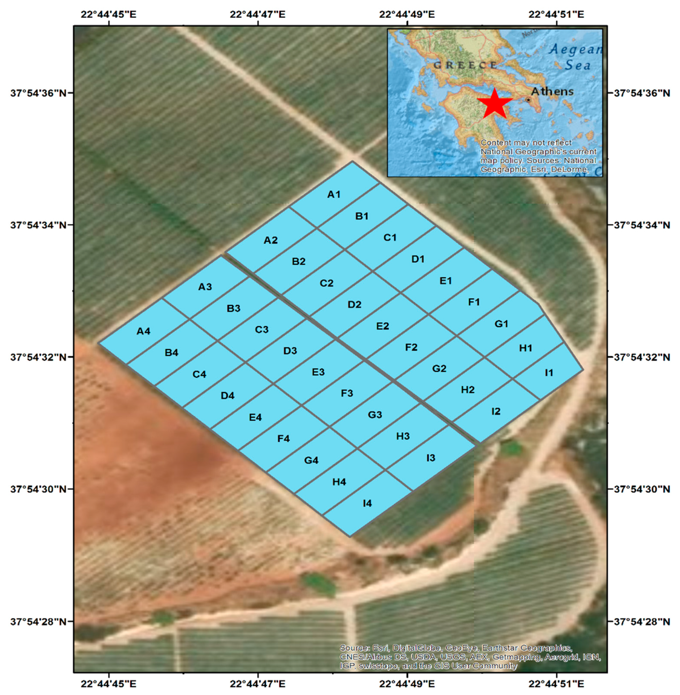
2.1. Field Site

The study was conducted at a commercial table grape vineyard located in Southern Greece during the 2015, 2016 and 2017 cultivation years (Figure 1). The vineyard was planted in 2006 with Vitis vinifera L. cv. Thompson seedless (37°54.532′ N, 22°44.798′ E, Corinth, Greece) at 1.4 ha. The variety was grafted onto 1103 Paulsen rootstock. The field exhibited variation in soil texture with two different soil types (sandy clay loam and clay loam). Table grapes were trained to a double cross arm trellis system and spaced at 1.8 m × 2.6 m. The vineyard received numerous vineyard operations (canopy management) to adjust the more vigorous vegetation. In addition, plant growth regulators and fertilizers were excessively used to reach commercial standards regarding the berry diameter and sugar content along with high yield. The vineyard was irrigated with approximately 2400 mm/ha, while 16 spraying applications of foliar fertilizers, plant protection products and crop growth regulators and 4 canopy management practices were applied on an annual basis. A regular grid of 36 cells (298–404 m² per cell) was set up to facilitate field sampling in order to assess crop vigour, yield and grape quality covering the total area, as shown in Figure 2. This methodology was also used by Tagarakis et al. (2013) and Farid et al. (2016) [40,41].

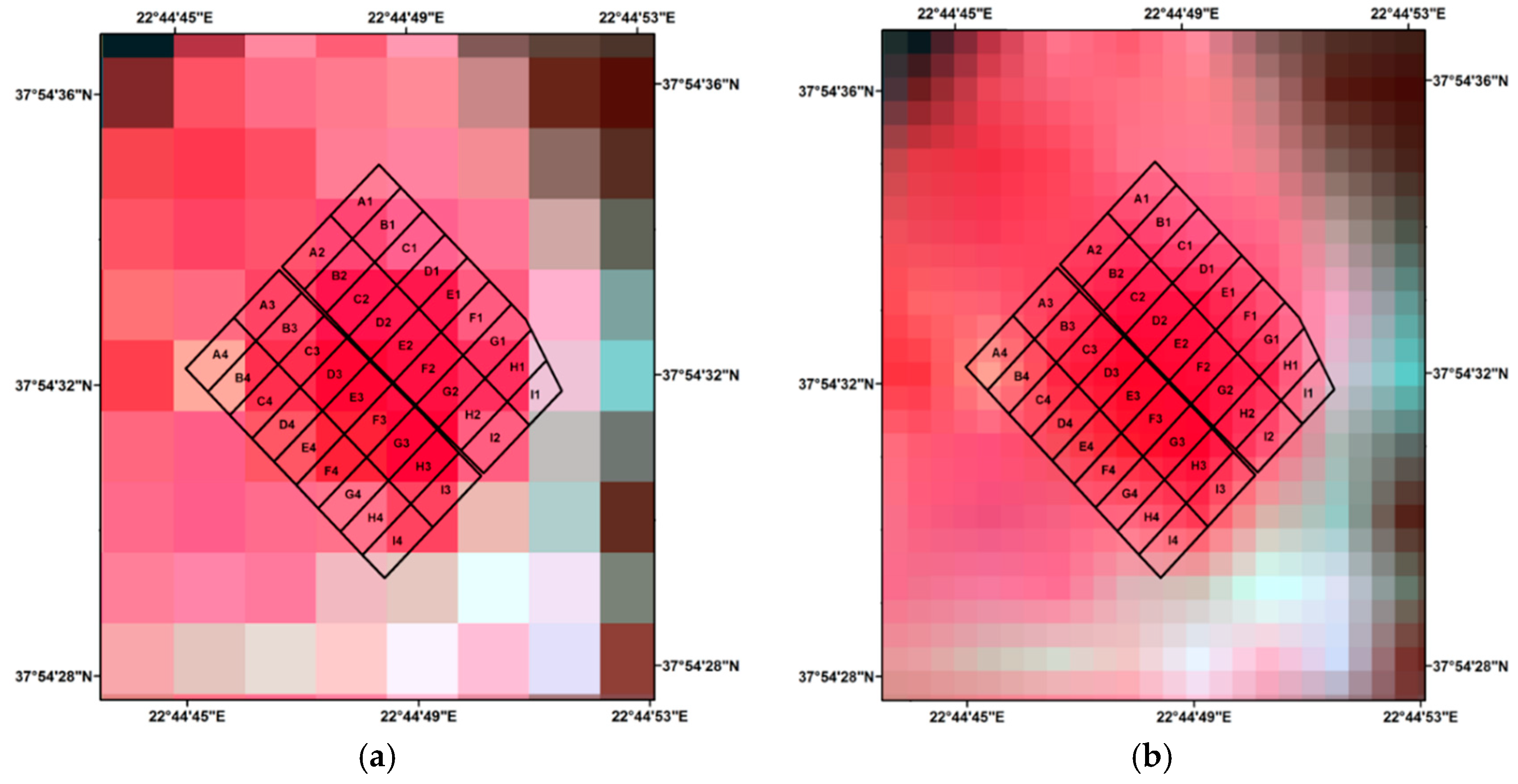
2.2. Remote Sensing Measurements

Crop vigour at 3 different developmental stages of the berry, namely (i) veraison (SV), (ii) mid of veraison (MV) and (iii) technological maturity (H), was assessed by measuring the Normalized Difference Vegetation Index (NDVI and the Green Normalized Difference Vegetation Index (GNDVI) (

Table 1. The spectral vegetation indices that were used in this study.

Spectral Vegetation Index	Equation	Bibliography
Normalized Difference Vegetation Index	$NDVI=\frac{NIR-RED}{NIR+RED}$	[43]
Green Normalized Difference Vegetation Index	$GNDVI=\frac{NIR-GREEN}{NIR+GREEN}$	[13]

). The selection of these specific development stages was due to the fact that during these stages, there is a rapid change in berry composition, such as sugar accumulation, which is reflected to final yield and quality [42]; several studies have found high correlations between SVIs and grape yield and quality characteristics at these developmental stages [20,23,39].

A Crop Circle proximal canopy sensor (ACS-470, Holland Scientific Inc., Lincoln, NE, USA) with the sensor located at a height of 1.5 m from the soil surface and 1.2 m horizontally from the vines was used to scan the side canopy area in order to assess crop vigour from proximal sensing, while Landsat 8 satellite imagery was used to assess it through satellite remote sensing. Three lenses with different band absorptions were used to calculate the above SVIs with the Crop Circle canopy sensor (550 nm—GREEN, 670 nm—RED and 760 nm—NIR), while Band 3 (GREEN), Band 4 (RED) and BAND 5 (NIR) from Landsat 8 were utilized for the calculation of the same SVIs. The reason for choosing the NIR wavelength was its high reflection in healthy leaves due to its relationship with many leaf structural features [44]. The red wavelength region was chosen because it presents strong absorption peaks for assessing the chlorophyll content [45], and some researchers have found that higher absorption in the green wavelength region increases the efficiency of plant photosynthetic activity compared to the red wavelength region [46]. Specifically, atmospherically corrected Landsat-8 satellite images (L2 products) were downloaded from the EarthExplorer, which is the satellite imagery data hub of the United States Geological Survey (USGS) agency (https://earthexplorer.usgs.gov/). The satellite imagery was resampled at a 10 m resolution by bilinear resampling in order to address the cell grid scale of the experimental site and to match the resolution of the freely available Sentinel-2A imagery (Figure 2). According to Zhang et al. (2018) similar results can be obtained between Sentinel-2A and Landsat-8 surface reflectance values by employing this method [47]. The measurement dates of the proximal canopy sensing and satellite sensing can be seen in

Table 2. Dates of acquisition of satellite and proximal sensing data.

Year	Satellite Imagery Dates	Proximal Sensing Dates
2015	16 July 2015 1 August 2015 2 September 2015	18 July 2015 30 July 2015 1 September 2015
2016	18 July 2016 3 August 2016 19 August 2016	16 July 2016 2 August 2016 17 August 2016
2017	14 July 2017 30 July 2017 15 August 2017	9 July 2017 26 July 2017 16 August 2017

.

2.3. Table Grape Measurements

The table grapes were hand harvested during 2–3 September 2015, 21–22 August 2016 and 16–17 August 2017. The actual yield was estimated during the harvest period by measuring the total number of bins per cell and multiplying it with the average bin weight of the harvested table grapes. Fifty berries were randomly taken in each vineyard cell at harvest by sampling five berries from one cluster per grapevine from a total of ten grapevines to assess berry and must parameters [48]. Berry diameters were estimated using the image analysis software, ImageJ 1.46r (Research Services Branch, NIMH, Bethesda, MD, USA). Specifically, each berry from the berry sample was placed in a custom made berry holder in an upright position and photographed with a digital camera (Konica Minolta Dimage Z6 (6.0 Mpixel), Minolta Co. Ltd., Osaka, Japan). The retrieved digital image was imported into ImageJ to calculate the Feret’s diameter of every berry, where the mean value for every berry sample lot was calculated. The individual berry fresh weight was determined for each sample of 50 berries per vineyard cell using a digital scale. The initial sample of 50 berries per cell was split in half to measure the deformation force in each of the 25 berries (deformation distance was taken as 1 mm based on Bourne (2002) [49]), and the rest of the 25 berries were used to measure the maximum force to detach the berry’s peduncle. The texture analysis was carried out in a Texture Analyser TA-XT2i (SMS, Surrey, UK). Upon completion of the non-destructive measurement, berry juice was extracted. The extracted juice was used to measure the total soluble solids (°Brix) with a digital refractometer (SR400), the total titratable acidity with a Fruit Acidity Meter GMK-708 (G-won Hitech Co., Seoul, Korea) and the pH with a pH meter AD8000 (Adwa Hungary Kft., Szeged, Hungary). The ripeness index is important for the table grape market and was calculated by dividing the total soluble solids (TSS) with the total titratable acidity (TTA), as presented in Equation (1) [50].

$$\mathrm{RI}=\frac{\mathrm{TSS}}{\mathrm{TTA}}$$

(1)

2.4. Map Construction and Statistical Analysis

The maps for vegetation images, yield and quality parameters for the three years of study were produced using ArcGIS 10.2 software (ESRI Inc., Redlands, CA, USA). For the assessment of the performance of satellite and proximal remote sensing on the estimation of table grape yield and quality, a statistical analysis was executed, including descriptive statistics, Pearson’s correlation and a regression model. The regression model analysis was performed only for the SVIs that presented the highest correlation for each approach and at a certain crop stage. The statistical analysis was conducted with statistical software (Statgraphics 16, StatPoint Technologies Inc., Warrenton, VA, USA).

3. Results

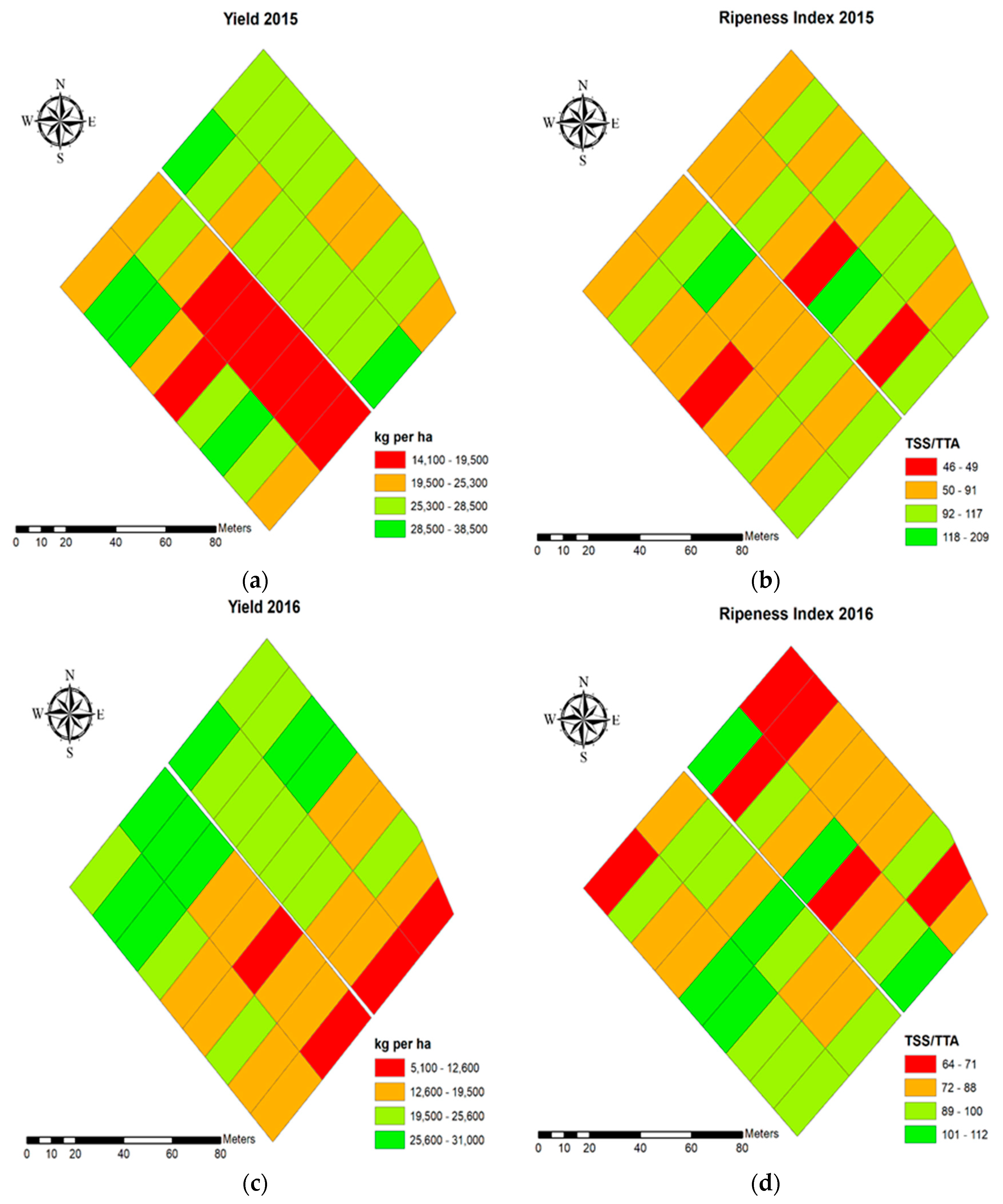
3.1. Descriptive Statistics

3.1.1. Table Grape Yield and Quality Characteristics

The table grape parameters presented different degrees of variation, as shown in Figure 3. Specifically, pH, total soluble solids and mean berry diameter presented coefficients of variance (CV) equal or lower than 10%. However, yield, berry detachment, total titratable acidity, berry deformation and the ripeness index presented higher CVs, with the highest values being given by yield and grape detachment (32% and 33%, respectively) (

Table 3. Descriptive statistics of the yield and quality characteristics of table grapes for the three years.

Table Grape Parameters	Min	Max	Mean	SD	CV (%)
Yield (kg/ha)	4518	38432	20612	6575	32%
Berry Detachment (N)	4.265	14.373	8.332	2.752	33%
pH	2.90	3.93	3.49	0.29	8%
Total Soluble Solids (TSS, °Brix)	15.7	23.2	18.6	1.3	7%
Total Titratable Acidity (TTA, %)	0.10	0.39	0.22	0.05	21%
Berry Diameter (mm)	19	28	23	2.215	10%
Berry Deformation (N/mm)	1.131	3.227	1.934	0.501	26%
TSS/TTA	45	209	87	21	24%

).

3.1.2. Satellite Based SVIs

GNDVI had a lower coefficient of variance compared to the NDVI for all different crop stages, while the CVs for both SVIs increased between the SV crop stage and the H stage (

Table 4. Descriptive statistics of the satellite based spectral vegetation indices (SVI) at different crop stages for the three years.

Satellite Sensing SVIs	Min	Max	Mean	SD	CV (%)
S NDVI SV	0.505	0.749	0.658	0.060	9%
S GNDVI SV	0.544	0.701	0.648	0.032	5%
S NDVI MV	0.509	0.769	0.649	0.066	10%
S GNDVI MV	0.544	0.710	0.641	0.038	6%
S NDVI H	0.493	0.762	0.649	0.068	10%
S GNDVI H	0.525	0.720	0.643	0.043	7%

SV: start of veraison crop stage, MV: middle of veraison crop stage, H: technological maturity crop stage.

). The SVIs had higher ranges of values near harvest, indicating that the top canopy’s vine leaves had higher photosynthetic rates near harvest [51,52].

3.1.3. Proximal Based SVIs

The proximal-based SVIs presented different coefficients of variance during the three developmental stages. Specifically, the NDVI presented the highest CV at the start of veraison, while the CVs of both SVIs decreased during the next crop stages. NDVI had the fastest drop in CV compared to GNDVI, with a value of 3% during the MV and H crop stages. Moreover, the highest values of SVIs occurred during the MV crop stage. This was due to the fact that that leaves that are found in the center of vine canopy are considered fully developed and present the highest photosynthetic activity compared to the others [51,52] (

Table 5. Descriptive statistics of the proximal-based spectral vegetation indices at different crop stages for the three years.

Proximal Sensing SVIs	Min	Max	Mean	SD	CV (%)
P NDVI SV	0.187	0.924	0.631	0.166	26%
P GNDVI SV	0.336	0.691	0.573	0.091	16%
P NDVI MV	0.717	0.824	0.793	0.022	3%
P GNDVI MV	0.339	0.718	0.615	0.068	11%
P NDVI H	0.623	0.836	0.775	0.027	3%
P GNDVI H	0.390	0.771	0.615	0.059	10%

SV: start of veraison crop stage, MV: middle of veraison crop stage, H: technological maturity crop stage.

).

3.2. Pearson’s Correlation

3.2.1. Satellite SVIs x Table Grapes Characteristics

Yield did not present correlations with NDVI nor GNDVI at any crop stage. Berry detachment correlated positively with both SVIs and had the highest correlation during the H crop stage. Moreover, GNDVI presented the highest correlation (r = 0.536, p < 0.01) among the two different SVIs with the berry detachment parameter. The same pattern of correlations was presented with the pH parameter, with GNDVI again showing the highest correlation (r = 0.537, p < 0.01). Both SVIs were negatively correlated with the total soluble solids, with the highest correlation during the MV stage (r = −0.362 and r = −0.373 for NDVI and GNDVI, respectively). There was no correlation between the TTA and the SVIs that were derived from satellite remote sensing. The berry diameter was correlated with both SVIs only at H stage, with GNDVI presenting the highest correlation (r = 0.522, p < 0.01). Berry deformation was correlated in all three crop stages with both SVIs, while GNDVI at the H crop stage presented the highest correlation with r = 0.629 (p < 0.01). The TSS/TTA ratio did not present any correlation with the SVIs at any crop stage. In conclusion, at harvest, GNDVI presented significant correlations at the p < 0.01 level with berry detachment, pH, total soluble solids, berry diameter and berry deformation, indicating that it can be used to assess the multiple crop yield and quality parameters at harvest (

Table 6. Pearson’s correlation matrix between the satellite-based spectral vegetation indices and the table grape yield and quality characteristics at different crop stages.

Satellite Sensing SVIs	Yield	Berry Detachment	pH	TSS	TTA	Berry Diameter	Berry Deformation	TSS/TTA
S NDVI SV	−0.016	0.140	0.155	−0.307 **	−0.043	0.131	0.222 *	−0.011
S GNDVI SV	0.083	0.153	0.161	−0.281 *	−0.056	0.172	0.244 *	−0.013
S NDVI MV	−0.136	0.182	0.254 **	−0.362 **	0.020	0.128	0.278 **	−0.085
S GNDVI MV	−0.069	0.225 *	0.306 **	−0.373 **	0.033	0.181	0.338 **	−0.097
S NDVI H	0.048	0.459 **	0.471 **	−0.335 **	0.008	0.424 **	0.551 **	−0.022
S GNDVI H	0.150	0.536 **	0.537 **	−0.322 **	0.006	0.522 **	0.629 **	−0.009

** Correlation is significant at the 0.01 level; * correlation is significant at the 0.05 level.

).

3.2.2. Proximal SVIs x Table Grapes Characteristics

Both SVIs presented correlations with table grape parameters at the SV and MV crop stages, while there were no correlations at harvest. Berry detachment presented a negative correlation with GNDVI at the SV and MV crop stages and positive with NDVI at the MV crop stage. The same pattern of correlations was presented with the pH parameter. In addition, the SVIs were correlated with TSS during the SV and MV crop stages with the highest correlations being presented in MV for NDVI (r = −0.255) and SV for GNDVI (r = 0.497). On the contrary, there was no correlation between TTA and the SVIs at all crop stages. The berry diameter was correlated with NDVI (SV and MV crop stages) and GNDVI (SV and MV crop stages) presenting the highest correlation with the latter at MV stage (r = 0.682, p < 0.01). Berry deformation presented the highest correlation with the GNDVI at MV crop stage. The TSS/TTA ratio presented a significant correlation only with NDVI at SV (r = 0.208, p < 0.05) (

Table 7. Pearson’s correlation matrix between the proximal-based spectral vegetation indices and the table grape yield and quality characteristics at different crop stages.

Proximal Sensing SVIs	Yield	Berry Detachment	pH	TSS	TTA	Berry Diameter	Berry Deformation	TSS/TTA
P NDVI SV	0.259 **	−0.037	−0.163	0.241 *	−0.173	0.014	−0.009	0.208 *
P GNDVI SV	0.085	−0.400 **	−0.627 **	0.497 **	−0.066	−0.395 **	−0.444 **	0.160
P NDVI MV	0.218 *	0.488 **	0.524 **	−0.255 **	−0.041	0.465 **	0.549 **	0.037
P GNDVI MV	−0.423 **	−0.572 **	−0.493 **	0.321 **	0.169	−0.682 **	−0.565 **	−0.121
P NDVI H	−0.115	−0.108	−0.146	0.102	0.002	−0.196 *	−0.156	0.014
P GNDVI H	−0.077	0.108	0.153	−0.039	−0.086	0.110	0.039	0.142

** Correlation is significant at the 0.01 level; * correlation is significant at the 0.05 level.

). Finally, GNDVI at the MV crop stage presented significant correlations at the p < 0.01 level with berry detachment, pH, total soluble solids, berry diameter and berry deformation, indicating that it could be used to assess multiple crop yield and quality parameters a few weeks before harvest.

3.3. Regression Analysis

GNDVI at harvest presented the highest correlations when compared with the NDVI for the different crop stages. For this reason, a linear regression analysis was performed using this SVI in order to evaluate its performance in assessing the yield and quality characteristics of table grapes for the highly correlated table grape characteristics. Accordingly, the assessment of proximal-sensed GNDVI at the MV crop stage to estimate the yield and quality characteristics of table grapes was performed through linear regression models only for the characteristics that had significant Pearson’s correlations. The results of this analysis are presented in the sub-sections below.

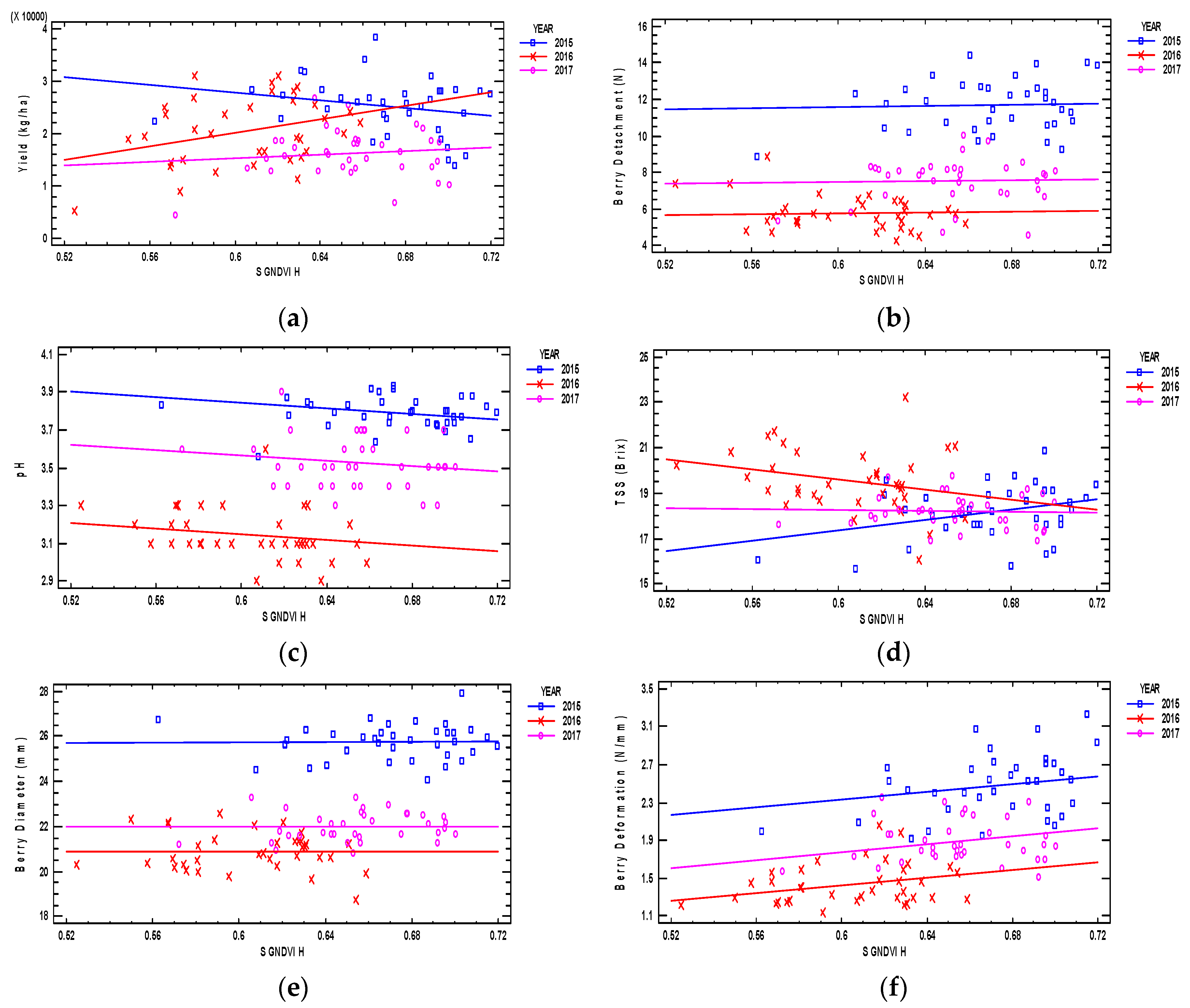
3.3.1. Satellite GNDVI H x Table Grape Characteristics

The regression models between satellite-derived GNDVI and table grape yield characteristics presented different degrees of accuracy. Specifically, the best fitted model was for the estimation of berry diameter (adjusted R² = 88%), while the other models’ accuracies were between 28% and 83%. The linear regression model that was developed for TSS had a coefficient of determination with adjusted R² of 28%, while the berry diameter model had an adjusted R² of 88%. Regarding the produced yield of table grapes, the model had a coefficient of determination equal to 33% (

Table 8. Regression model of correlated crop parameters with satellite-derived GNDVI at the harvest crop stage.

Regression Model	Year	Adjusted R2	RMSE
Yield = 50389 – 37530 × S GNDVI H	2015	33%	5382 kg/ha
Yield = −18,473 + 64276 × S GNDVI H	2016
Yield = 5379 + 16583 × S GNDVI H	2017
Berry Detachment = −2.14 + 20.95 × S GNDVI H	2015	83%	1.13 N
Berry Detachment = 13.86 − 13.77 × S GNDVI H	2016
Berry Detachment = 0.24 + 11.52 × S GNDVI H	2017
pH = 4.31 − 0.79 × S GNDVI H	2015	83%	0.12
pH = 3.61 − 0.79 × S GNDVI H	2016
pH = 4.03 − 0.79 × S GNDVI H	2017
TSS = 6.12 + 18.27 × S GNDVI H	2015	28%	1.10 °Brix
TSS = 25.15 − 9.55 × S GNDVI H	2016
TSS = 16.71 + 2.34 × S GNDVI H	2017
Berry Diameter = 24.7 + 1.5 × S GNDVI H	2015	88%	0.8 mm
Berry Diameter = 20 + 1.5 × S GNDVI H	2016
Berry Diameter = 21 + 1.5 × S GNDVI H	2017
Berry Deformation = 0.21 + 3.44 × S GNDVI H	2015	77%	0.24 N/mm
Berry Deformation = −0.58 + 3.44 × S GNDVI H	2016
Berry Deformation = −0.3 + 3.44 × S GNDVI H	2017

The values of adjusted R² and RMSE refer to all three years of this study.

and Figure 4).

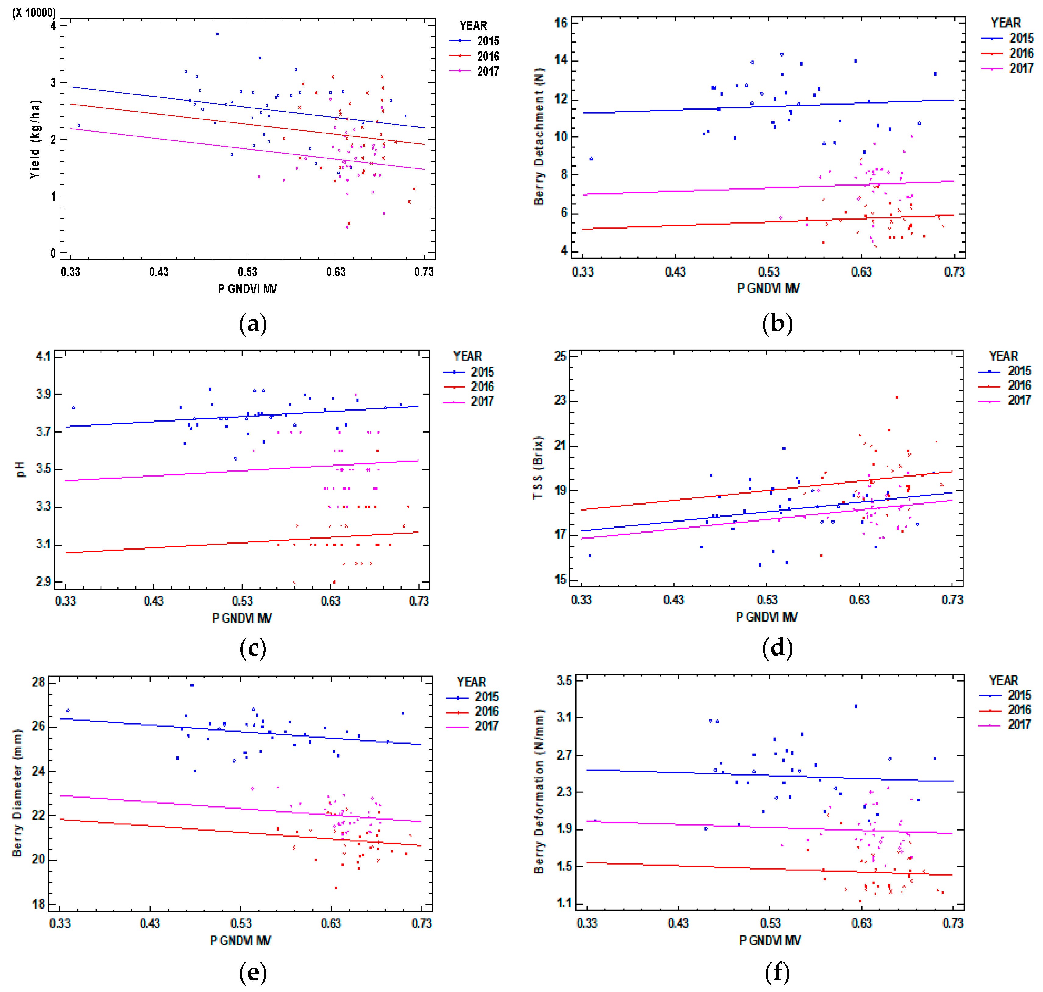
3.3.2. Proximal GRVI MV x Table Grape Characteristics

The linear regression models of table grape yield and quality characteristics with proximal sensed GNDVI at the MV crop stage presented coefficients of determination ranging between 26% and 89%. The berry diameter regression model had the highest coefficient of determination with an adjusted R² of 89% and the lowest was for estimating TSS (adjusted R² = 26%). The yield estimation model had a coefficient of determination of 31% (

Table 9. Regression model of correlated crop parameters with proximal-derived GRVI at the middle of veraison crop stage.

Regression Model	Year	Adjusted R2	RMSE
Yield = 34965 − 17742 × P GNDVI MV	2015	31%	5450 kg/ha
Yield = 31970 − 17742 × P GNDVI MV	2016
Yield = 27654 - 17742 × P GNDVI MV	2017
Berry Detachment = 10.68 + 1.78 × P GNDVI MV	2015	81%	1.21 N
Berry Detachment = 4.61 + 1.78 × P GNDVI MV	2016
Berry Detachment = 6.41 + 1.78 × P GNDVI MV	2017
pH = 3.64 + 0.27 × P GNDVI MV	2015	83%	0.12
pH = 2.97 + 0.27 × P GNDVI MV	2016
pH = 3.34 + 0.27 × P GNDVI MV	2017
TSS = 15.78 + 4.31 × P GNDVI MV	2015	26%	1.12 °Brix
TSS = 16.74 + 4.31 × P GNDVI MV	2016
TSS = 15.43 + 4.31 × P GNDVI MV	2017
Berry Diameter = 27.4 − 3 × P GNDVI MV	2015	89%	0.7 mm
Berry Diameter = 22.8 − 3 × P GNDVI MV	2016
Berry Diameter = 23.9 − 3 × P GNDVI MV	2017
Berry Deformation = 2.66 − 0.33 × P GNDVI MV	2015	72%	0.21 N/mm
Berry Deformation = 1.65 − 0.33 × P GNDVI MV	2016
Berry Deformation = 2.1 − 0.33 × P GNDVI MV	2017

The values of adjusted R² and RMSE refer to all three years of this study.

and Figure 5).

4. Discussion

All the yield and quality characteristics of the table grapes presented high CV values except for the berry diameter and total soluble solids. It is worth mentioning that the market value of Thompson seedless table grapes is based on the total soluble solids and berry diameter. Due to this, many agricultural operations, like the spraying of crop growth regulators are focused on producing homogenized products in accordance with to the aforementioned parameters. The SVIs presented correlations with specific yield and quality characteristics. Particularly, they were only correlated with yield, berry detachment, berry diameter, berry deformation, pH and total soluble solids. Similar results have also been found by other researchers [39,53], while there have been no other studies presenting any correlations of SVIs with berry deformation and berry detachment. However, the correlation of these two parameters with other yield and quality characteristics is also in accordance with other studies on mechanical properties of berries [54,55,56]. In detail, the satellite-based SVIs presented positive correlations with all of the aforementioned characteristics, except total soluble solids, during all developmental stages, while there were correlations between proximal-sensed SVIs with the same variables for the different crop stages. This is explained by the numerous operations (i.e., trimming) that took place during vine growth and affected the side canopy of the vine leaves. This study is aligned with Fountas et al. (2014) who stated that many field operations in vineyards, like in this vineyard, may affect the correlations of SVIs with the yield and quality parameters of grapes [39].

The highest correlations between the SVIs and the table grape yield and quality characteristics were presented at different crop stages for each of the two remote sensing methods. Specifically, the SVIs that were derived through proximal sensing had the highest correlations with table grape yield characteristics during the middle of veraison, while the satellite-derived SVIs presented their highest correlations during harvest. The latter is in accordance with Sun et al. (2017), who found that the best crop stage for estimating wine grape yield from satellite-derived data is before harvest, while Garcia-Estevez et al. (2017) found that the highest correlation of NDVI derived from proximal sensing with yield parameters of wine grapes was at veraison [57,58]. Thus, higher resolution data, such as proximal sensing data, can provide earlier crop yield and quality estimations compared to medium resolution remote sensing data. Landsat 8, with its small spatial resolution of 30 m, is a good and cheap approach, but the new satellites, such as Sentinel 2, that provide freely available data of higher resolution, are expected to facilitate this procedure. Moreover, this is explained by the physiology of the vines. Specifically, the vine leaves are developed as the vine shoots grow, resulting in more mature leaves being found near the trunk. This means that the more photosynthetically active leaves are found near the trunk at the beginning of vine development, while as the vine grows to senescence, these leaves are found at the edge of the shoot [51,52]. Consequently, the leaves that are at the side canopy, which are measured with proximal sensing, have higher values of SVIs earlier in the growing season compared to the satellite-based SVIs that measure the photosynthetic activity of the top canopy leaves. This is an indication that the use of proximal sensing can present earlier and more accurate estimations of important yield and quality characteristics without being affected by soil background effects and lower resolution, which is the case for the satellite SVIs.

Furthermore, it was found that the satellite-based GNDVI at harvest provided comparable results and, in some cases, better results for the estimation of table grape yield and quality characteristics when compared to proximal-based SVIs. This finding comes in accordance with Tattaris et al. (2016) study, in which the satellite imagery provided better results on estimating yield when compared with aerial and proximal remote sensing [59]. This was also presented by Yang et al. (2013) who found that the use of high resolution satellite imagery can provide comparable results with aerial data of higher resolution [60].

Moreover, according to this study, there are higher correlations between satellite-derived GNDVI and proximal-derived GNDVI with table grape yield characteristics when compared with NDVI. Hall and Wilson (2013) found that SVIs, like the EVI (Enhanced Vegetation Index), perform better than NDVI in estimating wine grape yield characteristics, thus supporting the findings of this study [61]. Moreover, the saturation of NDVI at high values had lower correlations with crop parameters, like the grapevine biomass and crop coefficient, resulting in lower estimations of crop yield characteristics and crop evapotranspiration [62,63]. Consequently, there is need to assess the performance of different SVIs in order to use the most appropriate method according to the variable being measured.

5. Conclusions

In this study, an assessment of different remote sensing methods (satellite and proximal) for the estimation of crop yield characteristics was conducted during three crop growing seasons (2015, 2016 and 2017) on a commercial table grape vineyard cultivated with Thompson Seedless variety grapes. Two different spectral vegetation indices were calculated based on the spectral information that was derived from the different methods. The statistical analysis indicated that proximal sensing resulted in higher accuracy in estimating crop yield characteristics when compared with satellite sensing-derived estimations. Proximal sensing provided higher correlations earlier in the growing season than the satellite sensing approach, suggesting that the first method can be used as a tool for on time scheduling of table grape yield and quality estimation.

This type of study is valuable, as non-destructive methods for crop quantitative and qualitative characteristics are increasing due to the benefits they provide to the end users (farmers, crop consultants, public bodies, etc.). Further research is needed to assess new spectral vegetation indices and sampling resolutions using different sensing methods (e.g., comparison of Unmanned Aerial Vehicle-based SVIs with proximal and satellite sensing SVIs).

References

1. Fresh Deciduous Fruit: World Markets and Trade (Apples, Grapes, & Pears). Available online: https://apps.fas.usda.gov/psdonline/circulars/fruit.pdf (accessed on 29 April 2018).
2. Strik, B.C. Growing Table Grapes. 32. Available online: http://smallfarms.oregonstate.edu/sites/default/files/publications/growing_table_grapes_ec1639_may_2011.pdf (accessed on 29 April 2018).
3. Rather, J.A.; Wani, S.H.; Haribhushan, A.; Bhat, Z.A. Influence of girdling, thinning and GA3 on fruit quality and shelf life of grape (Vitis vinifera) cv. perlette. Elixir Agric. 2011, 41, 5731–5735. [Google Scholar]
4. Sen, F.; Oksar, R.; Kesgin, M. Effects of Shading and Covering on ‘Sultana Seedless’ Grape Quality and Storability. J. Agric. Sci. Technol. 2016, 18, 245–254. [Google Scholar]
5. Tehrani, M.M.; Kamgar-Haghighi, A.A.; Razzaghi, F.; Sepaskhah, A.R.; Zand-Parsa, S.; Eshghi, S. Physiological and yield responses of rainfed grapevine under different supplemental irrigation regimes in Fars province, Iran. Sci. Hortic. 2016, 202, 133–141. [Google Scholar] [CrossRef]
6. Hussein, M.A.; Abd-elall, E.H. Attempts to Improve Berry Quality of flame seedless Grapevines. Egypt. J. Hortic. 2017, 44, 235–244. [Google Scholar] [CrossRef]
7. Moran, M.S.; Inoue, Y.; Barnes, E.M. Opportunities and limitations for image-based remote sensing in precision crop management. Remote Sens. Environ. 1997, 61, 319–346. [Google Scholar] [CrossRef]
8. Mondal, P.; Basu, M. Adoption of precision agriculture technologies in India and in some developing countries: Scope, present status and strategies. Prog. Nat. Sci. 2009, 19, 659–666. [Google Scholar] [CrossRef]
9. Panda, S.S.; Ames, D.P.; Panigrahi, S. Application of Vegetation Indices for Agricultural Crop Yield Prediction Using Neural Network Techniques. Remote Sens. 2010, 2, 673–696. [Google Scholar] [CrossRef] [Green Version]
10. Thenkabail, P.S.; Smith, R.B.; De Pauw, E. Hyperspectral Vegetation Indices and Their Relationships with Agricultural Crop Characteristics. Remote Sens. Environ. 2000, 71, 158–182. [Google Scholar] [CrossRef]
11. Gitelson, A.; Merzlyakb, M.N. Quantitative estimation of chlorophyll-u using reflectance spectra: Experiments with autumn chestnut and maple leaves. J. Photochem. Photobiol. B Biol. 1994, 22, 247–252. [Google Scholar] [CrossRef]
12. Pena-Barragan, J.M.; Lopez-Granados, F.; Jurado-Exposito, M.; Garcia-Torres, L. Spectral discrimination of Ridolfia segetum and sunflower as affected by phenological stage. Weed Res. 2006, 46, 10–21. [Google Scholar] [CrossRef] [Green Version]
13. Chang, J.; Clay, D.E.; Dalsted, K.; Clay, S.; O’Neill, M. Corn (Zea mays L.) Yield Prediction Using Multispectral and Multidate Reflectance. Agron. J. 2003, 95, 1447–1453. [Google Scholar] [CrossRef]
14. Ranjitha, G.; Srinivasan, M.R.; Rajesh, A. Detection and Estimation of Damage Caused by Thrips Thrips tabaci (Lind) of Cotton Using Hyperspectral Radiometer. Agrotechnology 2014, 3. [Google Scholar] [CrossRef]
15. Genc, H.; Genc, L.; Turhan, H.; Smith, S.E.; Nation, J.L. Vegetation indices as indicators of damage by the sunn pest (Hemiptera: Scutelleridae) to field grown wheat. Afr. J. Biotechnol. 2008, 7, 173–180. [Google Scholar]
16. Jia, L.; Yu, Z.; Li, F.; Gnyp, M.; Koppe, W.; Bareth, G.; Miao, Y.; Chen, X.; Zhang, F. Nitrogen Status Estimation of Winter Wheat by Using an IKONOS Satellite Image in the North China Plain. In Computer and Computing Technologies in Agriculture V; Li, D., Chen, Y., Eds.; Springer: Berlin/Heidelberg, Germany, 2012; Volume 369, pp. 174–184. ISBN 978-3-642-27277-6. [Google Scholar]
17. Li, F.; Gnyp, M.L.; Jia, L.; Miao, Y.; Yu, Z.; Koppe, W.; Bareth, G.; Chen, X.; Zhang, F. Estimating N status of winter wheat using a handheld spectrometer in the North China Plain. Field Crops Res. 2008, 106, 77–85. [Google Scholar] [CrossRef]
18. Glaser, J.; Casas, J.; Copenhaver, K.; Mueller, S. Development of a broad landscape monitoring system using hyperspectral imagery to detect pest infestation. In Proceedings of the IEEE2009 First Workshop on Hyperspectral Image and Signal Processing: Evolution in Remote Sensing, Grenoble, France, 26–28 August 2009; pp. 1–4. [Google Scholar]
19. Huete, A.; Didan, K.; Miura, T.; Rodriguez, E.; Gao, X.; Ferreira, L. Overview of the radiometric and biophysical performance of the MODIS vegetation indices. Remote Sens. Environ. 2002, 83, 195–213. [Google Scholar] [CrossRef]
20. Hall, A.; Lamb, D.W.; Holzapfel, B.P.; Louis, J.P. Within-season temporal variation in correlations between vineyard canopy and winegrape composition and yield. Precis. Agric. 2011, 12, 103–117. [Google Scholar] [CrossRef]
21. Baluja, J.; Diago, M.P.; Goovaerts, P.; Tardaguila, J. Assessment of the spatial variability of anthocyanins in grapes using a fluorescence sensor: Relationships with vine vigour and yield. Precis. Agric. 2012, 13, 457–472. [Google Scholar] [CrossRef]
22. Joshi, N.; Baumann, M.; Ehammer, A.; Fensholt, R.; Grogan, K.; Hostert, P.; Jepsen, M.R.; Kuemmerle, T.; Meyfroidt, P.; Mitchard, E.T.A.; et al. A Review of the Application of Optical and Radar Remote Sensing Data Fusion to Land Use Mapping and Monitoring. Remote Sens. 2016, 8, 70. [Google Scholar] [CrossRef]
23. Hall, A.; Lamb, D.W.; Holzapfel, B.; Louis, J. Optical remote sensing applications in viticulture—A review. Aust. J. Grape Wine Res. 2002, 8, 36–47. [Google Scholar] [CrossRef]
24. Gascon, F.; Bouzinac, C.; Thépaut, O.; Jung, M.; Francesconi, B.; Louis, J.; Lonjou, V.; Lafrance, B.; Massera, S.; Gaudel-Vacaresse, A.; et al. Copernicus Sentinel-2A Calibration and Products Validation Status. Remote Sens. 2017, 9, 584. [Google Scholar] [CrossRef]
25. Vaudour, E.; Carey, V.A.; Gilliot, J.M. Digital zoning of South African viticultural terroirs using bootstrapped decision trees on morphometric data and multitemporal SPOT images. Remote Sens. Environ. 2010, 114, 2940–2950. [Google Scholar] [CrossRef]
26. Rodríguez, J.R.; Miranda, D.; Álvarez, C.J. Application of satellite images to locate and inventory vineyards in the designation of origin “Bierzo” in Spain. Trans. ASABE 2006, 49, 277–290. [Google Scholar] [CrossRef]
27. Semmens, K.A.; Anderson, M.C.; Kustas, W.P.; Gao, F.; Alfieri, J.G.; McKee, L.; Prueger, J.H.; Hain, C.R.; Cammalleri, C.; Yang, Y.; et al. Monitoring daily evapotranspiration over two California vineyards using Landsat 8 in a multi-sensor data fusion approach. Remote Sens. Environ. 2016, 185, 155–170. [Google Scholar] [CrossRef] [Green Version]
28. Johnson, L.; Roczen, D.; Youkhana, S.; Nemani, R.; Bosch, D. Mapping vineyard leaf area with multispectral satellite imagery. Comput. Electron. Agric. 2003, 38, 33–44. [Google Scholar] [CrossRef]
29. Kandylakis, Z.; Karantzalos, K. Precision viticulture from multitemporal, multispectral very high resolution satellite data. ISPRS Int. Arch. Photogramm. Remote Sens. Spat. Inf. Sci. 2016, 41, 919–925. [Google Scholar] [CrossRef]
30. Borgogno-Mondino, E.; Lessio, A.; Tarricone, L.; Novello, V.; de Palma, L. A comparison between multispectral aerial and satellite imagery in precision viticulture. Precis. Agric. 2018, 19, 195–217. [Google Scholar] [CrossRef]
31. Matese, A.; Gennaro, S.F.D. Technology in Precision Viticulture: A State of the Art Review. Available online: https://www.dovepress.com/technology-in-precision-viticulture-a-state-of-the-art-review-peer-reviewed-fulltext-article-IJWR (accessed on 29 April 2018).
32. Erena, M.; Montesinos, S.; Portillo, D.; Alvarez, J.; Marin, C.; Fernandez, L.; Henarejos, J.M.; Ruiz, L.A. Configuration and specifications of an unmanned aerial vehicle for precision agriculture. ISPRS Int. Arch. Photogramm. Remote Sens. Spat. Inf. Sci. 2016, XLI-B1, 809–816. [Google Scholar] [CrossRef]
33. Marçal, A.; Gonçalves, J.; Cunha, M. Analysis of the temporal signature of vineyards in Portugal using VEGETATION. In Proceedings of the 26th EARSeL Symposium, New Developments and Challenges in Remote Sensing, Warsaw, Poland, 29 May–2 June 2006; Millpress: Rotterdam, The Netherlands, 2007; pp. 377–384. [Google Scholar]
34. Cerovic, Z.G.; Moise, N.; Agati, G.; Latouche, G.; Ben Ghozlen, N.; Meyer, S. New portable optical sensors for the assessment of winegrape phenolic maturity based on berry fluorescence. J. Food Compos. Anal. 2008, 21, 650–654. [Google Scholar] [CrossRef]
35. Llorens, J.; Gil, E.; Llop, J.; Escolà, A. Ultrasonic and LIDAR Sensors for Electronic Canopy Characterization in Vineyards: Advances to Improve Pesticide Application Methods. Sensors 2011, 11, 2177–2194. [Google Scholar] [CrossRef] [PubMed] [Green Version]
36. Del-Moral-Martínez, I.; Rosell-Polo, J.R.; Company, J.; Sanz, R.; Escolà, A.; Masip, J.; Martínez-Casasnovas, J.A.; Arnó, J. Mapping Vineyard Leaf Area Using Mobile Terrestrial Laser Scanners: Should Rows be Scanned On-the-Go or Discontinuously Sampled? Sensors 2016, 16, 119. [Google Scholar] [CrossRef] [PubMed]
37. Gatti, M.; Dosso, P.; Maurino, M.; Merli, M.C.; Bernizzoni, F.; José Pirez, F.; Platè, B.; Bertuzzi, G.C.; Poni, S. MECS-VINE®: A New Proximal Sensor for Segmented Mapping of Vigor and Yield Parameters on Vineyard Rows. Sensors 2016, 16, 2009. [Google Scholar] [CrossRef] [PubMed]
38. Kazmierski, M.; Glémas, P.; Rousseau, J.; Tisseyre, B. Temporal stability of within-field patterns of NDVI in non irrigated Mediterranean vineyards. OENO One 2011, 45, 61. [Google Scholar] [CrossRef]
39. Fountas, S.; Anastasiou, E.; Balafoutis, A. The influence of vine variety and vineyard management on the effectiveness of canopy sensors to predict winegrape yield and quality. In Proceedings of the International Conference of Agricultural Engineering, Zurich, Switzerland, 6–10 July 2014; p. 8. [Google Scholar]
40. Tagarakis, A.; Liakos, V.; Fountas, S.; Koundouras, S.; Gemtos, T.A. Management zones delineation using fuzzy clustering techniques in grapevines. Precis. Agric. 2013, 14, 18–39. [Google Scholar] [CrossRef]
41. Farid, H.U.; Bakhsh, A.; Ahmad, N.; Ahmad, A.; Mahmood-Khan, Z. Delineating site-specific management zones for precision agriculture. J. Agric. Sci. 2016, 154, 273–286. [Google Scholar] [CrossRef]
42. Sonnekus, N. Development and Change that Occurs in Table Grape Berry Composition during Growth. Ph.D. Thesis, Stellenosch University, Stellenbosch, South Africa, 2015. [Google Scholar]
43. Huete, A. A comparison of vegetation indices over a global set of TM images for EOS-MODIS. Remote Sens. Environ. 1997, 59, 440–451. [Google Scholar] [CrossRef]
44. Vescovo, L.; Wohlfahrt, G.; Balzarolo, M.; Pilloni, S.; Sottocornola, M.; Rodeghiero, M.; Gianelle, D. New spectral vegetation indices based on the near-infrared shoulder wavelengths for remote detection of grassland phytomass. Int. J. Remote Sens. 2012, 33, 2178–2195. [Google Scholar] [CrossRef] [PubMed]
45. Wu, C.; Niu, Z.; Tang, Q.; Huang, W. Estimating chlorophyll content from hyperspectral vegetation indices: Modeling and validation. Agric. For. Meteorol. 2008, 148, 1230–1241. [Google Scholar] [CrossRef]
46. Terashima, I.; Fujita, T.; Inoue, T.; Chow, W.S.; Oguchi, R. Green Light Drives Leaf Photosynthesis More Efficiently than Red Light in Strong White Light: Revisiting the Enigmatic Question of Why Leaves are Green. Plant Cell Physiol. 2009, 50, 684–697. [Google Scholar] [CrossRef] [PubMed] [Green Version]
47. Zhang, H.K.; Roy, D.P.; Yan, L.; Li, Z.; Huang, H.; Vermote, E.; Skakun, S.; Roger, J.-C. Characterization of Sentinel-2A and Landsat-8 top of atmosphere, surface, and nadir BRDF adjusted reflectance and NDVI differences. Remote Sens. Environ. 2018. [Google Scholar] [CrossRef]
48. Neto, F.J.D.; Tecchio, M.A.; Junior, A.P.; Vedoato, B.T.F.; Lima, G.P.P.; Roberto, S.R. Effect of ABA on colour of berries, anthocyanin accumulation and total phenolic compounds of ‘Rubi’ table grape (Vitis vinifera). Aust. J. Crop Sci. 2017, 11, 199–205. [Google Scholar] [CrossRef]
49. Bourne, M.C. Food Texture and Viscosity: Concept and Measurement, 2nd ed.; Academic Press: London, UK, 2002; ISBN 0-12-119062-5. [Google Scholar]
50. Muñoz-Robredo, P.; Robledo, P.; Manríquez, D.; Molina, R.; Defilippi, B.G. Characterization of Sugars and Organic Acids in Commercial Varieties of Table Grapes. Chil. J. Agric. Res. 2011, 71, 452–458. [Google Scholar] [CrossRef] [Green Version]
51. Escalona, J.M.; Flexas, J.; Bota, J.; Medrano, H. Distribution of leaf photosynthesis and transpiration within grapevine canopies under different drought conditions. Vitis 2003, 42, 57–64. [Google Scholar]
52. Bertamini, M.; Nedunchezhian, N. Photosynthetic functioning of individual grapevine leaves (Vitis vinifera L. cv. Pinot noir) during ontogeny in the field. Vitis 2003, 42, 13–17. [Google Scholar]
53. Martinez-Casasnovas, J.A.; Agelet-Fernandez, J.; Arno, J.; Ramos, M.C. Analysis of vineyard differential management zones and relation to vine development, grape maturity and quality. Span. J. Agric. Res. 2012, 10, 326. [Google Scholar] [CrossRef] [Green Version]
54. Esgici, R.; Özdemir, G.; Pekitkan, G.; Eliçin, K.; Öztürk, F.; Sessiz, A. Engineering Properties of the Şire Grape (Vitis vinifera L. cv.). Scientific Papers. Ser. B Horticult. 2017, LXI, 195–204, Print ISSN 2285-5653. [Google Scholar]
55. Giacosa, S.; Torchio, F.; Rio Segade, S.; Giust, M.; Tomasi, D.; Gerbi, V.; Rolle, L. Selection of a Mechanical Property for Flesh Firmness of Table Grapes in Accordance with an OIV Ampelographic Descriptor. Am. J. Enol. Vitic. 2014, 65, 206–214. [Google Scholar] [CrossRef]
56. Fernandes, J.C.; Cobb, F.; Tracana, S.; Costa, G.J.; Valente, I.; Goulao, L.F.; Amâncio, S. Relating Water Deficiency to Berry Texture, Skin Cell Wall Composition, and Expression of Remodeling Genes in Two Vitis vinifera L. Varieties. J. Agric. Food Chem. 2015, 63, 3951–3961. [Google Scholar] [CrossRef] [PubMed]
57. Sun, L.; Gao, F.; Anderson, M.; Kustas, W.; Alsina, M.; Sanchez, L.; Sams, B.; McKee, L.; Dulaney, W.; White, W.; et al. Daily Mapping of 30 m LAI and NDVI for Grape Yield Prediction in California Vineyards. Remote Sens. 2017, 9, 317. [Google Scholar] [CrossRef]
58. García-Estévez, I.; Quijada-Morín, N.; Rivas-Gonzalo, J.C.; Martínez-Fernández, J.; Sánchez, N.; Herrero-Jiménez, C.M.; Escribano-Bailón, M.T. Relationship between hyperspectral indices, agronomic parameters and phenolic composition of Vitis vinifera cv. Tempranillo grapes: Hyperspectral indices, agronomic parameters and phenolic composition of V. vinifera. J. Sci. Food Agric. 2017, 97, 4066–4074. [Google Scholar] [CrossRef] [PubMed]
59. Tattaris, M.; Reynolds, M.P.; Chapman, S.C. A Direct Comparison of Remote Sensing Approaches for High-Throughput Phenotyping in Plant Breeding. Front. Plant Sci. 2016, 7, 1131. [Google Scholar] [CrossRef] [PubMed]
60. Yang, C.; Everitt, J.H.; Du, Q.; Luo, B.; Chanussot, J. Using High-Resolution Airborne and Satellite Imagery to Assess Crop Growth and Yield Variability for Precision Agriculture. Proc. IEEE 2013, 101, 582–592. [Google Scholar] [CrossRef]
61. Hall, A.; Wilson, M.A. Object-based analysis of grapevine canopy relationships with winegrape composition and yield in two contrasting vineyards using multitemporal high spatial resolution optical remote sensing. Int. J. Remote Sens. 2013, 34, 1772–1797. [Google Scholar] [CrossRef]
62. Junges, A.H.; Fontana, D.C.; Anzanello, R.; Bremm, C. Normalized difference vegetation index obtained by ground-based remote sensing to characterize vine cycle in Rio Grande do Sul, Brazil. Ciênc. E Agrotecnol. 2017, 41, 543–553. [Google Scholar] [CrossRef] [Green Version]
63. Er-Raki, S.; Rodriguez, J.C.; Garatuza-Payan, J.; Watts, C.J.; Chehbouni, A. Determination of crop evapotranspiration of table grapes in a semi-arid region of Northwest Mexico using multi-spectral vegetation index. Agric. Water Manag. 2013, 122, 12–19. [Google Scholar] [CrossRef]
Figure 1. Satellite image of the table grapes in the commercial vineyard.
Agriculture 08 00094 g001
Figure 2. Landsat 8 false color images with (a) 30 m and (b) 10 m resolution.
Agriculture 08 00094 g002
Figure 3. Maps of (a) yield 2015, (c) yield 2016, (e) yield 2017, (b) ripeness Index 2015, (d) ripeness Index 2016 and (f) ripeness Index 2017. The value ranges of all table grape parameters are presented according to the four quartiles.
Agriculture 08 00094 g003aAgriculture 08 00094 g003b
Figure 4. Scatterplots of S GNDVI H with (a) yield, (b) berry detachment, (c) pH, (d) total soluble solids, (e) berry diameter, and (f) derry deformation.
Agriculture 08 00094 g004
Figure 5. Scatterplots of P GNDVI MV with (a) yield, (b) berry detachment, (c) pH, (d) total soluble solids, (e) berry diameter, and (f) berry deformation.
Agriculture 08 00094 g005