Design and Implementation of a Rainfed Matrix for Cotton

Abstract

Global production of agricultural products must continue to increase if shortages are to be avoided. While irrigated production is substantial since water available for both current and future production is limited, rainfed production will become increasingly important. In-season weather variability results in instability in rainfed production and in order to gain information on the mechanisms involved and their potential mitigation, it is important to monitor production over a range of possible environmental scenarios. We designed and implemented a rain matrix experimental approach for cotton based on a series of sequential plantings coupled with a rain-simulation protocol. The rain matrix in two years produced 56 growing environments with rain and thermal variability and 44 yield:environment comparisons. The yield:rain relationship was not strong (R² = 0.35) Analysis of heat units over the matrix indicated (1) heat units varied with planting date and (2) heat units were sufficient to achieve maturity. Plantings reached maturity with <1250 heat units and reached maturity before a lethal freeze. The rain matrix design increased the number of yield:environment comparisons in a single year and though it is subject to undefined thermal interactions, may prove useful in understanding rainfed cotton production.

1. Introduction

Rainfed crop production accounts for approximately 84% of production and is clearly an essential component of global agriculture. Irrigated land accounts for roughly 36% of production from only 16% of land. The expansion of irrigated production is increasingly limited due to the lack of water resources available for agricultural production [1]. Thus, the expansion of rainfed production systems appears to be an essential component of efforts to increase agricultural production [2].

While increased yields are generally the most obvious outcome of irrigation, the stabilizing effect of even limited irrigation on yields is an important and under-appreciated aspect of irrigated production [3,4,5].

The improvement and stabilization of yield in rainfed production systems are needed if agricultural production is to be an increasingly important means of providing agricultural products to an expanding population.

All agricultural production is subject to environmental variation that has the potential to reduce yields relative to the crop potential. Temperature and water significantly influence crop productivity. While temperature cannot be managed in-season, the choice of crops and growing seasons within an environment are management decisions that are used to reduce the adverse effects of temperature. Germplasm that is optimized to specific thermal environments is another means of mitigating adverse effects of thermal variation [6,7].

Water is perhaps as important as temperature in determining the performance of cropping systems and, fortunately, management of water by producers is possible, to varying degrees, in virtually all production systems. Production of crops in regions where rain resources are sufficient for sustainable yields is common practice, but increasing demands for crop production have pushed cropping into regions where water resources are marginal.

In a cropping system, as the difference between rain amounts and crop water need increases, irrigation increases and stabilizes productivity. The stabilization of yield is an aspect of irrigated crop production that is often difficult to assess but that may become important as existing systems convert from irrigated to rainfed. As water in an agricultural system is reduced, variability generally increases adding to the difficulty inherent in agricultural production [8].

The improvement of rainfed cotton in the region will require a greater understanding of the strengths and weaknesses of the current rainfed production systems. The variable nature of rain will become an even more significant source of variation in cotton performance as the stabilizing effect of, even minimal, irrigation is removed [9].

The pattern and amount of rain during a season, while broadly predictable seasonally on a decadal scale, is largely unpredictable on a day-to-day scale within a given season. The growth and development of the crop over the course of a season results in variation in the water requirement of the crop and, thus, its water status on a daily basis and the effect of a given rain has to be seen in the context of its growth and development. A given rain event, depending on its amount and timing relative to the crop, can significantly affect the crop or alternatively have almost no effect on the crop. Given the complexity of the relationships among rain amounts, temporal distribution of rain and the growth and development of the crop prior to the rain, identification of rainfed management strategies becomes complex.

Our goal in this study is to establish an experimental rainfed matrix that increases the variability in rain amount, rain timing, environmental conditions and management options over which the performance of the cotton crop can be monitored. Increasing the number of rain patterns that the crop experiences during a growing season is the ultimate goal of the rainfed matrix approach that we have implemented. Each rain pattern produced in the rainfed matrix is associated with a set of environmental conditions and crop management settings that ultimately are expressed as yield (cotton fiber).

The rainfed matrix approach is based upon using a combination of multiple planting dates, the amount and pattern of rain associated with each planting, and a series of rain simulations to enhance variation in rain patterns across multiple cotton crops at a single location within a single year. The use of multiple planting dates within a single annual environmental pattern will result in cotton plants of various ages being subject to naturally-occurring rain events at different growth stages and environmental conditions. This produces multiple “cotton crops” in a single season each of which has a unique rain and weather pattern.

In Lubbock, Texas, we have identified seven potential cotton crop seasons in a single year using seven plantings at 2-week intervals. The seven potential cotton crop seasons fall within the 238-day growing period available for cotton in the region. A recent publication defines this approach in greater detail [10].

2. Materials and Methods

The study was carried out in the spring, summer, and fall of 2016 and 2017 at the USDA/ARS research laboratory in Lubbock TX (33°35′36″ N, 101°54′00″ W). The field was fertilized prior to planting in accord with standard regional recommendations based on soil samples to a 20 cm depth. Weeds were controlled by hand hoeing of the plots and periodic applications of glyphosate.

Pre-planting soil moisture was measured gravimetrically in the field by a series of soil cores (0 to 1 m-depth). Plant available soil water content was calculated based on the soil characterization. As a result of winter rain and a small (<50 mm) irrigation on March 1 in both years, the initial soil moisture content at the first planting was near field capacity with ~100 mm of plant available water.

The rain matrix consisted of seven sequential plantings of cotton (Gossypium hirsutum L., Deltapine 1612) in each of two years. Each planting was 16 rows, 20 m in length with 1-m row spacing. For each of the seven planting dates there were four plots, each representing a simulated-rain treatment based on a rain decile. The seven plantings with four rain simulations per planting resulted in a total of 28 plots per year with 28 patterns and amounts of study-rain over the course of each growing season. The sequential plantings were planted on an approximately 2-week interval between 1 April and 11 July in 2016 and 2017 (

Table 1. 2016 Summary.

Planting Number	Planting Date (DOY)	Maturity Date (DOY) DAP	Environment-Heat Units (Planting to Freeze)	Crop-Heat Units (Planting to Maturity)	Natural Rain Simulated Total	Yield kg/ha	Water Productivity kg/mm
1	1 April 2016 (92)	30 August 2016 (242) 150	1428	1100	Based on schedule	NA
2	15 April 2016 (106)	30 August 2016 (242) 136	1416	1100	Based on schedule	NA
3	1 May 2016 (122)	4 September 2016 (247) 125	1382	1100	Based on schedule	NA
4	25 May 2016 (146)	8 September 2016 (251) 105	1297	1052	300	658	2.19
5	8 June 2016 (159)	23 September 2016 (266) 106	1215	1078	254	651	2.56
6	22 June 2016 (173)	4 November 2016 (308) 134	1068	1065	264	867	3.28
7	6 July 2016 (187)	20 November 2016 (324) 137 freeze	913	913	264	324

and

Table 2. 2017 Summary.

Planting Number	Planting Date (DOY)	Maturity Date (DOY) DAP	Environment-Heat Units (Planting to Freeze)	Crop-Heat Units (Planting to Maturity)	Natural Rain + Simulated Total	Yield kg/ha	Water Productivity kg/mm
1	5 April 2017 (95)	26 August 2017 (238) 143	1331	1186	359	1617	4.5
2	19 April 2017 (109)	29 August 2017 (241) 132	1296	1156	344	1235	3.5
3	2 May 2017 (122)	19 September 2017 (262) 140	1267	1281	354	1753	4.95
4	16 May 2017 (136)	9 October 2017 (282) 146	1222	1310	404	1430	3.5
5	31 May 2017 (151)	23 October 2017 (296) 145	1148	1249	389	1236	3.17
6	22 June 2017 (173)	28 October 2017 (301) 128	943	1030	380	760	2.07
7	11 July 2017 (192)	28 October 2017 (301) 128	753	829	380	100

). The planting dates were specified at 2-week intervals but varied due to rain events that, in some instances, made planting on a specific date impractical. The cotton was planted at a target rate of 10 seeds per meter (98,800 seeds per hectare) under a center pivot irrigation system with sprinkler nozzles at 1-m spacing approximately 1-m above the ground. Immediately after planting, an irrigation of 6 mm of water was applied to the planting with the pivot irrigation system. This was done to ensure sufficient moisture for germination and emergence.

There were seven plantings in each year of the study resulting in a total of 14 plantings for the study. A hailstorm on 6 June 2016 resulted in the loss of the first three plantings. Rain and weather data were collected for all 14 plantings while crop yield and study-rain were only available for a total of 11 plantings (four through seven in 2016 and one through seven in 2017).

We have defined three measures of rain in this study; (1) rain, (2) simulated-rain and (3) study-rain which is the sum of rain and simulated-rain and represents all water on the crop. Rain events during the season were measured with a tipping bucket rain gauge. Simulated-rain amounts were established by the pivot irrigation controller and verified with tipping bucket rain gauges installed in the field. Study-rain (rain + simulated rain) was measured over the interval between the dates of planting and crop maturity.

The date of crop maturity was defined in terms of 60% of open bolls. An end-of-season lethal freeze (>6 h <0 °C) on November 20 in 2016 and 2017 marked the end of the growing season for all plantings. End of season yield was measured using combination of hand harvests and a 4-row cotton stripper. Seed cotton was ginned on a table-top gin to produce lint yield.

Heat units were calculated on a daily basis based on the equation:

Heat units for a day = (Max air temp − Min air temp)/2 − 15.5 °C.

(1)

If the Max temp < 15.5 °C the heat units for that day = 0

3. Results/Discussion

3.1. Development of a Sequential Planting Matrix

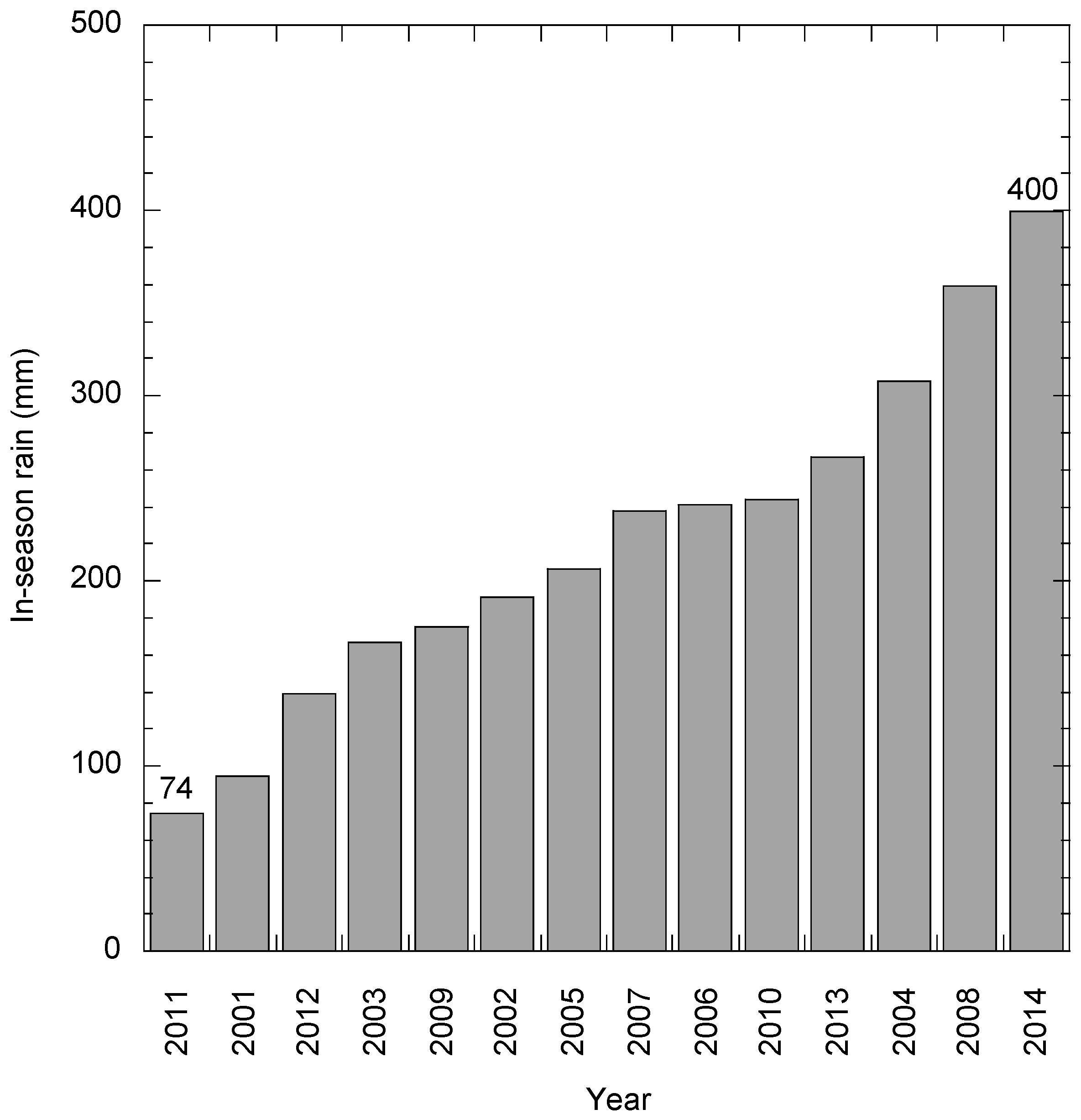
Reductions in agricultural water resources and the desire to increase production are creating a need for improved rainfed cotton production systems in the southern high plains region of Texas. Year-to-year rain variability makes rainfed production studies potentially difficult and time consuming. Progress in understanding rainfed cotton production will be enhanced by information on the response of cotton to multiple growing environments. With one planting a year, at a single location, a cotton crop will produce one yield value that is linked to a single growing environment and a single seasonal rain amount. Figure 1 shows the rain distribution that would have occurred if a cotton crop had been planted on 15 May and grown for 150 days in the 14 years of the historic rain period. Such a single planting would have produced in-season rain amounts between 74 and 400 mm and 14 yield:environment pairs. It is apparent that the rate of data generation under such a system would be slow.

The limitations described above indicate the need for an experimental design to increase the number of yield:environment pairs that can be produced over time. In this study, a rainfed matrix based on historic weather and agronomic knowledge for cotton in the region was used to increase the number of yield:environment comparisons that can be made in a growing season. The rainfed matrix consists of two elements: (1) A series of sequential cotton plantings to allow for the observation of cotton performance across a range of environments (primarily rain and temperature) and (2) a simulated-rain protocol. The coupling of simulated-rain and the sequential plantings creates the matrix. The rainfed matrix system required the following: (1) Design of a planting matrix based on the potential crop seasons that could be evaluated at the study site and (2) development of a rain simulation protocol.

The first step in implementation of a sequential planting-based rainfed cotton matrix is the determination of the number of successful plantings (e.g., yield producing) that can be made in a given year at the study location. Cotton is produced in the interval between lethal low temperatures in the spring and fall, and the length of this interval provides a basis to define a series of cotton plantings dates within a given year. Rainfed cotton on the southern high plains of Texas requires <150 days to reach maturity and when planted in the interval between early April (~DOY 90) and late June (~DOY 174) it will probably produce yield. Since cotton planted on DOY 174 will require <150 days to reach maturity, the end of the cropping season would be DOY 324. Thus, the potential cropping season for cotton in the region would be the 234-day period between 1 April and 20 November. This 234-day period for cotton production provides the basis for using multiple plantings in a single year to increase the number of yield:environment comparisons that can be made in a single year. Given seven sequential plantings on a two-week interval between DOY 90 to DOY 174, each planting would be provided a 22-week crop period to reach maturity. Using this approach, a single year at Lubbock, TX can be partitioned into the following seven potential crop periods for cotton; (#1) DOY 90–240, (#2) DOY 104–254, (#3) DOY 118–268, (#4) DOY 132–282, (#5) DOY 146–296, (#6) DOY 160–310, (#7) DOY 174–324. It is noted that the DOY 324 date is certainly at the extreme end of the cotton season and, in at least some years, the end-of-season lethal freeze would occur prior to DOY 324. These seven crop periods provide the basis for the sequential plantings component of a cotton rainfed matrix.

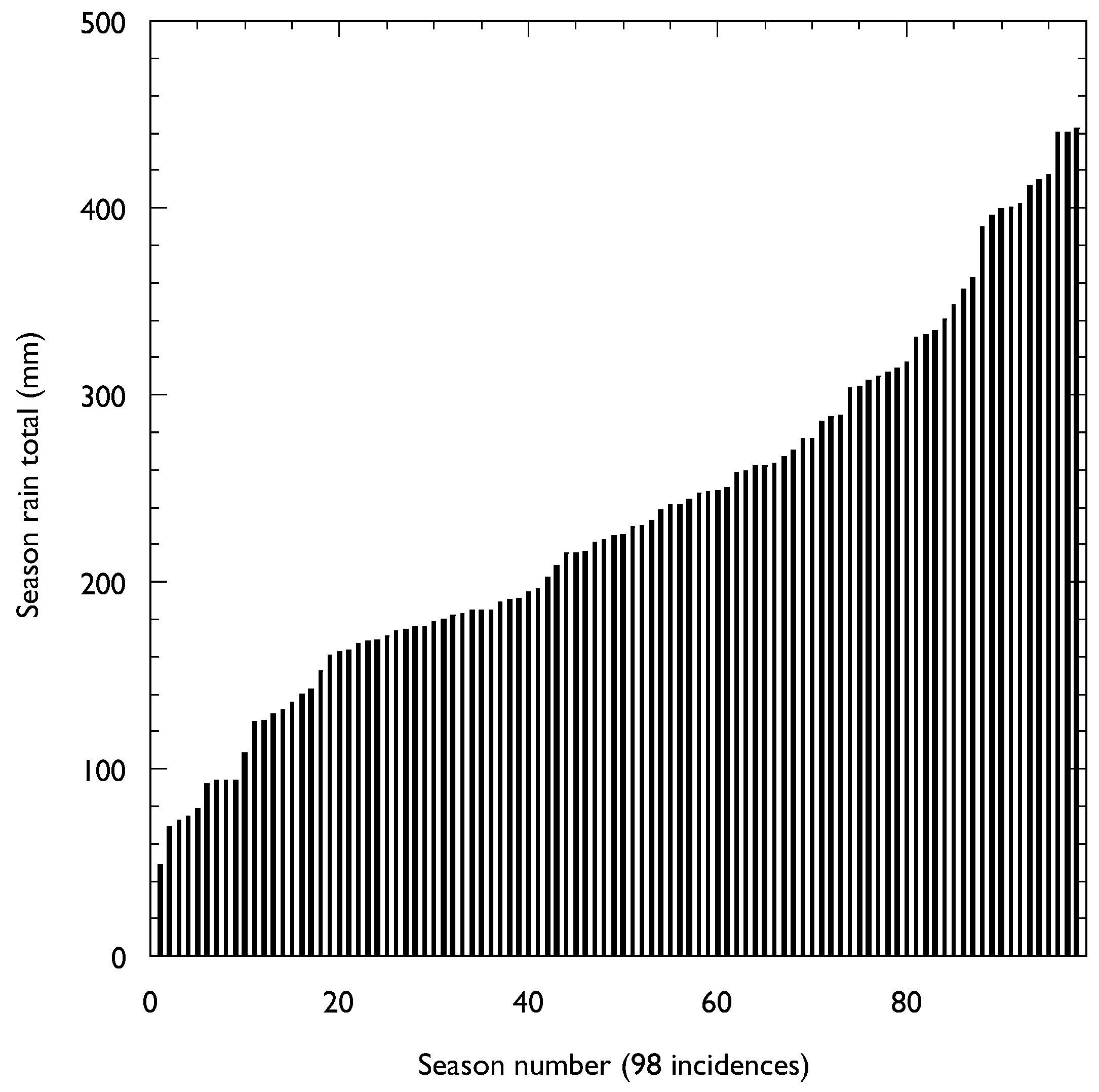
The historic pattern of rain during each of seven-planting periods/year over the 14-year period from 2001 to 2014 in Lubbock, Texas (TX) is shown in Figure 2. The planting periods were defined to cover the typical cotton season from DOY 90 to DOY 324 (1 April to 20 November). This 33-week period was subdivided into seven, 22-week cropping periods of 150 days each based upon sequential plantings at 2-week intervals. A series of seven plantings, executed over the 14-year historic interval, would produce seven rain:environment pairs per year for a total of 98 rain:environment pairs. Each of the rain periods can be characterized in terms of its end point value (total rain over 150 days) and a temporal rain pattern consisting of a 22-week time series. An analysis of the temporal pattern of the dataset is beyond the scope of this study and will be addressed in the future. The sequential planting series increases the data year by a factor of seven compared to a single planting per year.

3.2. A Rain Simulation Protocol

The previous section described the use of a sequential planting matrix to increase the number of yield:environment pairs that can be observed in a single season. In any rainfed field study there will be wet years and dry years, and the experiment must be repeated over a number of years to experience the range of rain for the site. In an effort to overcome the “one rain pattern/planting limitation”, a rain simulation protocol with four simulated-rain entries was added to the planting series creating a rain matrix.

The extent to which the rain matrix design increases the data that can be generated in a single season is described thusly. Over the 14-year historic period of the study; a single cotton planting/year would produce a total of 14 yield:rain pairs, a seven-planting series would produce a total of 98 yield:rain pairs, and a rain matrix with four rain simulations would produce 392 yield:rain pairs. Over a more realistic 5-year field study, a rain matrix with seven-plantings and four rain simulations would produce a total of 140 yield:rain pairs.

There are several options for generating simulated-rain patterns. One could simply adopt a reactive “wait and see” approach by adding simulated-rain as the season develops based on some understanding of where the crop is relative to rain at that point in the season. Another approach could involve a stochastic approach with pattern of simulated-rain that is applied regardless of the rain amounts in the preceding weeks. Our approach is to use a 14-year historic analysis of rain for the location to create a weekly simulated-rain pattern to determine amounts of rain.

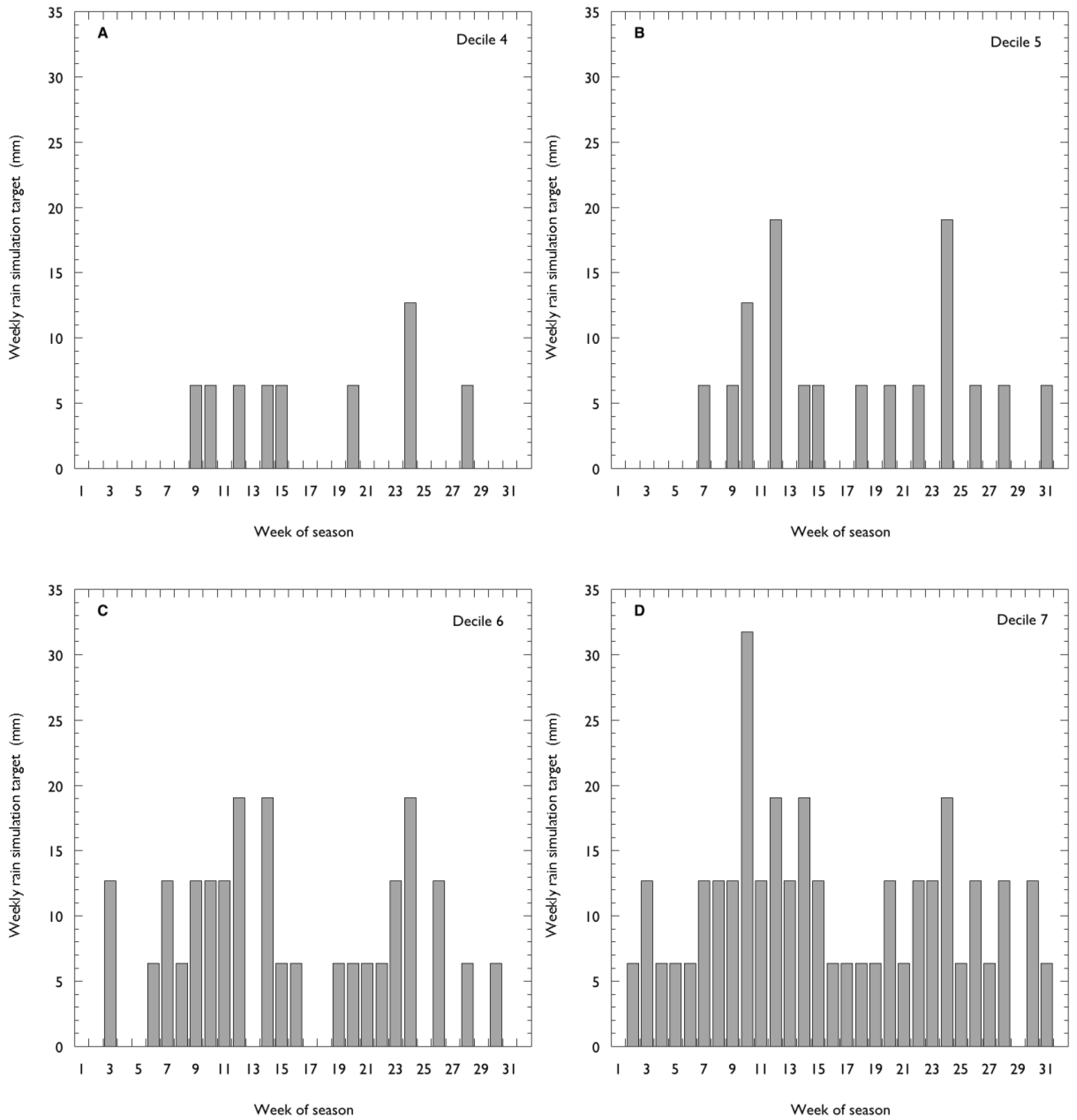
The rain simulations in this study were derived from the 14-year rain history at the site based on a series of seven sequential plantings possible for a cotton crop. For each of the 14 years in the study, the 238-day growing period between DOY 90 and DOY 328 (1 April to 24 November) was divided into 34 sequential 1-week intervals. This produced 14 rain amounts for each of the 34 weeks of the growing period for a total of 476 rain events. The distribution of rain amounts over the 14 years was determined for each of the 34 weeks. The rain amounts for each week were broken into deciles and the fourth, fifth, sixth and seventh decile amounts were chosen for rain simulations. The selection of the mid-range of the rain amounts (deciles 4 through 7) for rain simulations was based on our interest in moderate rain years compared to extremely dry and wet production years of the region. Each decile group consists of a series of 34 weekly rain amounts to be used as study-rain targets and provide the basis for weekly irrigations to supplement rain during the season. During the season, the weekly difference between rain and the study-rain targets determines if irrigation is applied or withheld. On a weekly interval, if rain < the study-rain target then irrigation is applied and if rain > the study-rain target irrigation is canceled. The study-rain targets for 34 weeks of the annual study period (1 April through 24 November) are shown for deciles 4 through 7 in the Figure 3. 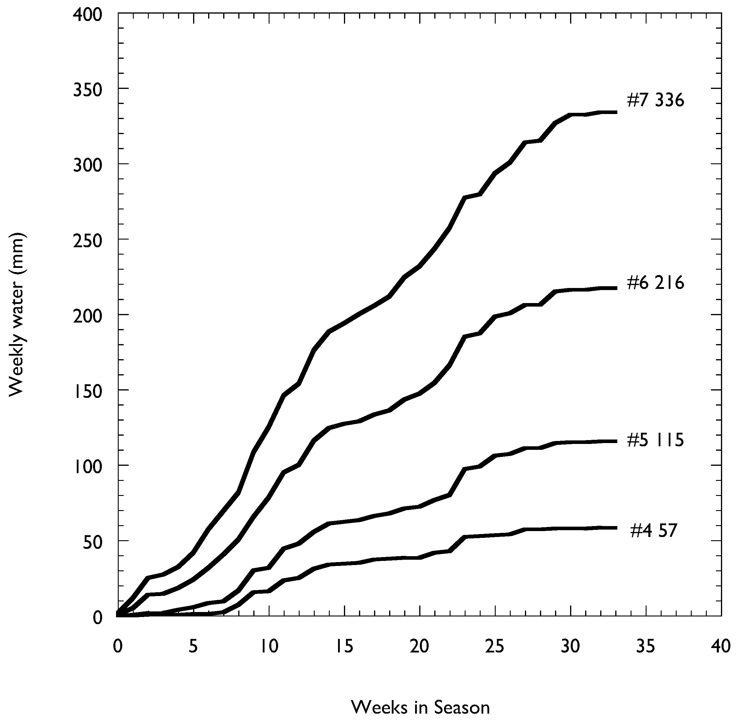Figure 4 shows the sum of the target amounts produced by the different deciles. The amounts, temporal distribution and number of study-rain targets vary across the treatment deciles. Simulated-rain generated by the 4th decile results in eight simulated-rain events with a total volume of 57 mm while the 7th decile produces 29 simulated-rain events with a total volume of 336 mm.

The study-rain patterns shown in the two figures represent the outcomes that would occur if there was no rain in a year. In a low rain year, the study-rain will be closer to the simulated-rain and in a higher rain year the contribution of simulated-rain to the study-rain is diminished. The use of decile-based rain simulations that are derived from relatively recent rain history for the location provides a rational basis for rain simulations that is relatively simple and reproducible.

3.3. How We Made Rain Simulations on the Matrix 2016 and 2017

The simulated rain applications were made once a week based on the rain simulation protocol whose derivation is described above. In weeks when rain at the site exceeded the amount called for by the rain simulation protocol, no irrigation occurred and, in weeks when rain was less than that specified in the protocol, the difference was applied by irrigation as simulated-rain. Rain simulations were carried out using a center pivot irrigation system with sprinkler heads designed to spread water across the plants and the inter-row space in a manner similar to a rain event.

The simulated-rain protocol was based on a set of decile study-rain targets described above. The procedure for generating the simulated-rain patterns for a planting is as follows. For each week of each 22-week crop period simulation, on day 7 of the simulation interval the measured rain at the site over the preceding 6 days was compared to the study-rain target amount for that week based on each of the four decile-based rain simulations. If the weekly rain at the site was greater than or equal to the study-rain target amount for that week, no action was taken. If the rain for the week was less than the study-rain target amount associated for that week, the difference was applied as simulated-rain. Due to the limits on the operation of the pivot irrigation device, each irrigation “call” resulted in the application of water in 6 mm increments. For instance, if the difference between rain for the week was <6 mm, 6 mm of irrigation was applied and if the weekly difference was >6 mm but less than or equal to 12 mm, 12 mm was applied. This procedure was followed for each of the four decile-based rain simulation treatments for each of the 22 weeks of the seven planting dates from planting to maturity. This procedure resulted in a total of 28 rain simulation treatments for each year.

The rain matrix was designed to improve our understanding of cotton performance under rainfed production conditions by increasing the range of environmental variation experience by the crop in a single growing season. The primary source of environmental variation is a series of planting dates that is enhanced with a simulated-rain events overlaid on the in-season rain producing a rain matrix for a year. The incorporation of rain simulations provides a mechanism to increase rain variability across the various plantings over a single season.

3.4. Study-Rain Targets

For each rain simulation there is an end-of-season target amount of study-rain (rain + simulated-rain), Figure 4. If there is no rain during the season for a given plot, the amount of water applied by for all simulations will match their rain targets. The decile-basis of the simulated rain protocol results in a distribution over time that would be bounded by the upper and lower limits of rain in dry and wet years. The study-rain amounts over the 14-year historic rain interval would fall in the range shown in Figure 5 for a sequential planting series.

In a season when rain exceeds the rain target value for a decile, the study-rain for the treatment will exceed its rain target. This can be accommodated by departing from the rain simulation protocol in response to large rain events. For example, a 50 mm rain event can be accommodated in a given decile by skipping two weeks of irrigation and then resuming the rain simulation. The goal of the rain simulation is to provide variability in rain over the season and as long as the natural and simulated-rain amounts are recorded, variation in study-rain is the result. The bias in the protocol is perhaps toward exceeding the rain targets, but over time the matrix protocol should allow the for a wider range of rain amounts (study-rain) than would be achieved by simply using rain at a location.

The ultimate utility of rain simulations is assessed in terms of their ability to create rain patterns that are representative of the rain distributions that comprise the rain history for a given crop at a location. There are really no “right or wrong” rain simulations, only those that work and those that do not. The goal of including rain simulations in a rain matrix approach is to increase the range of rain amounts and patterns that can be assessed in a single season.

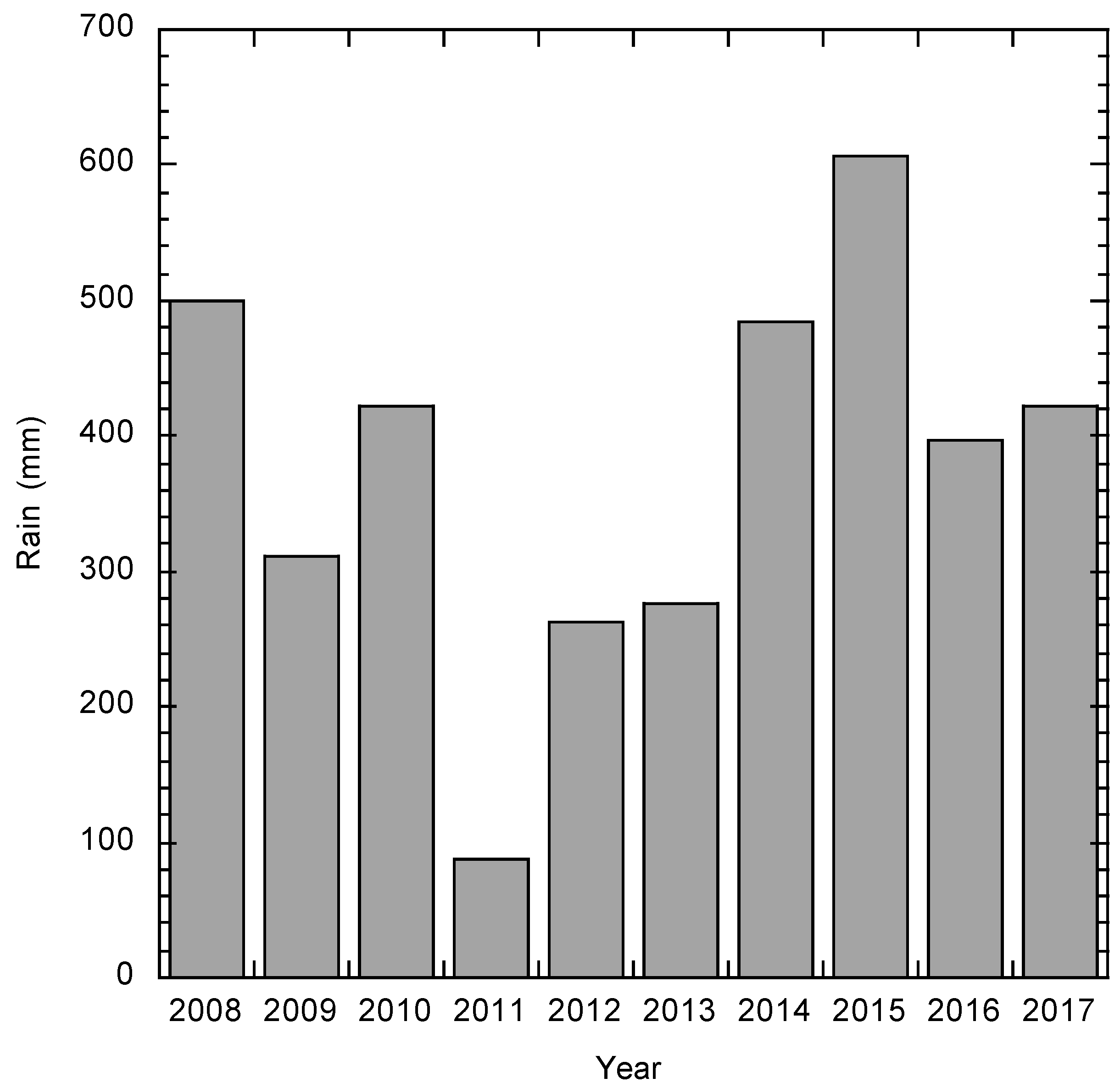
3.5. Rain during the 2016 and 2017 Study Interval

Rain during the entire study interval from 15 March to 15 November was 431 mm for 2016 and 401 mm for 2017. The total amounts are in the mid-range of rain at the location over the past 10 years with four years of lesser rain and four of greater amounts (Figure 5).

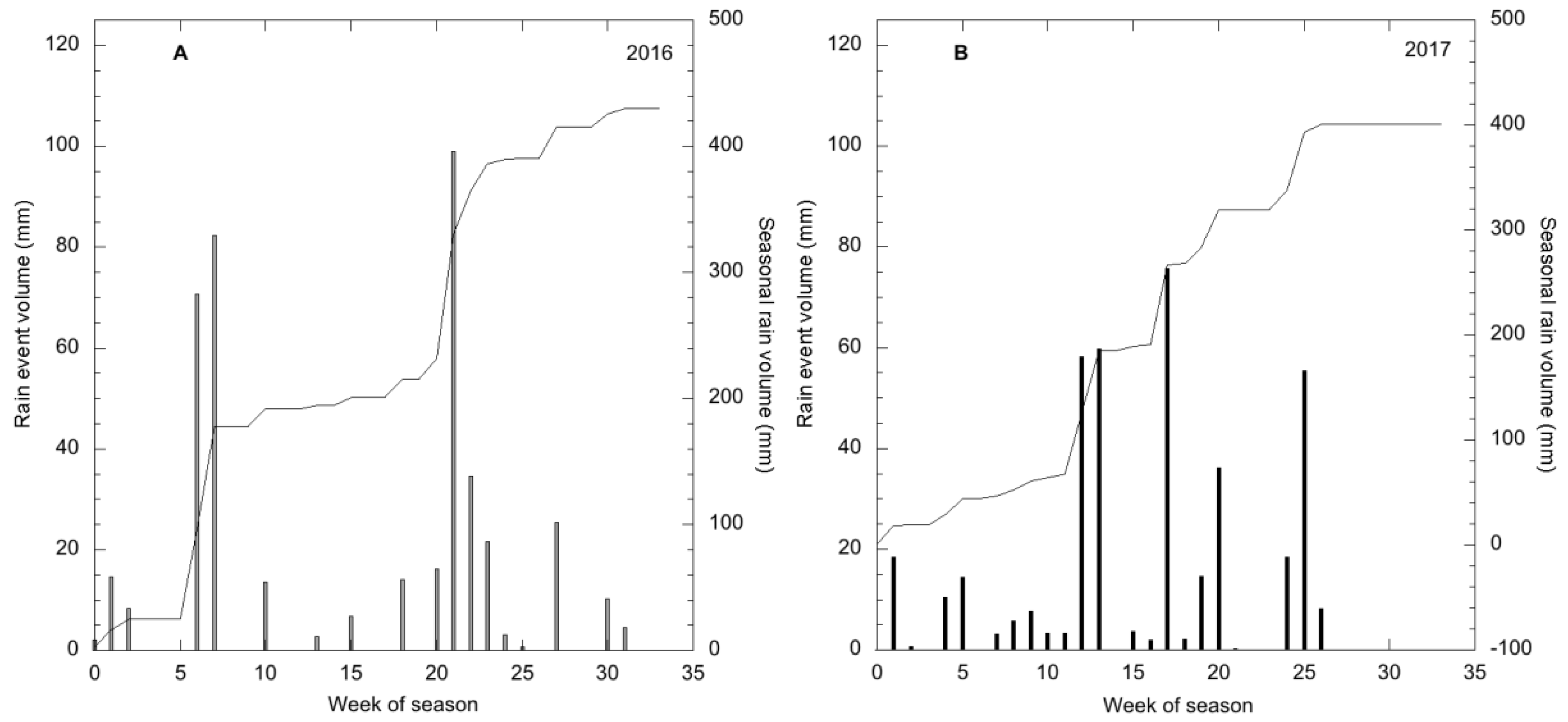
The gross weather patterns for the year are most useful when viewed in an agrocentric context relating to what happened and when in the 150-day period over which an individual cotton planting transitioned from a seed to a cotton boll. The rain patterns during the experimental period in 2016 and 2017 are shown in Figure 6. Rain in 2016 was roughly centered on the 35-week period, while in 2017 there were two clusters of rain events in early and later half of the season. While we believe that the patterns of rain over time are probably important, they are beyond the scope of this report.

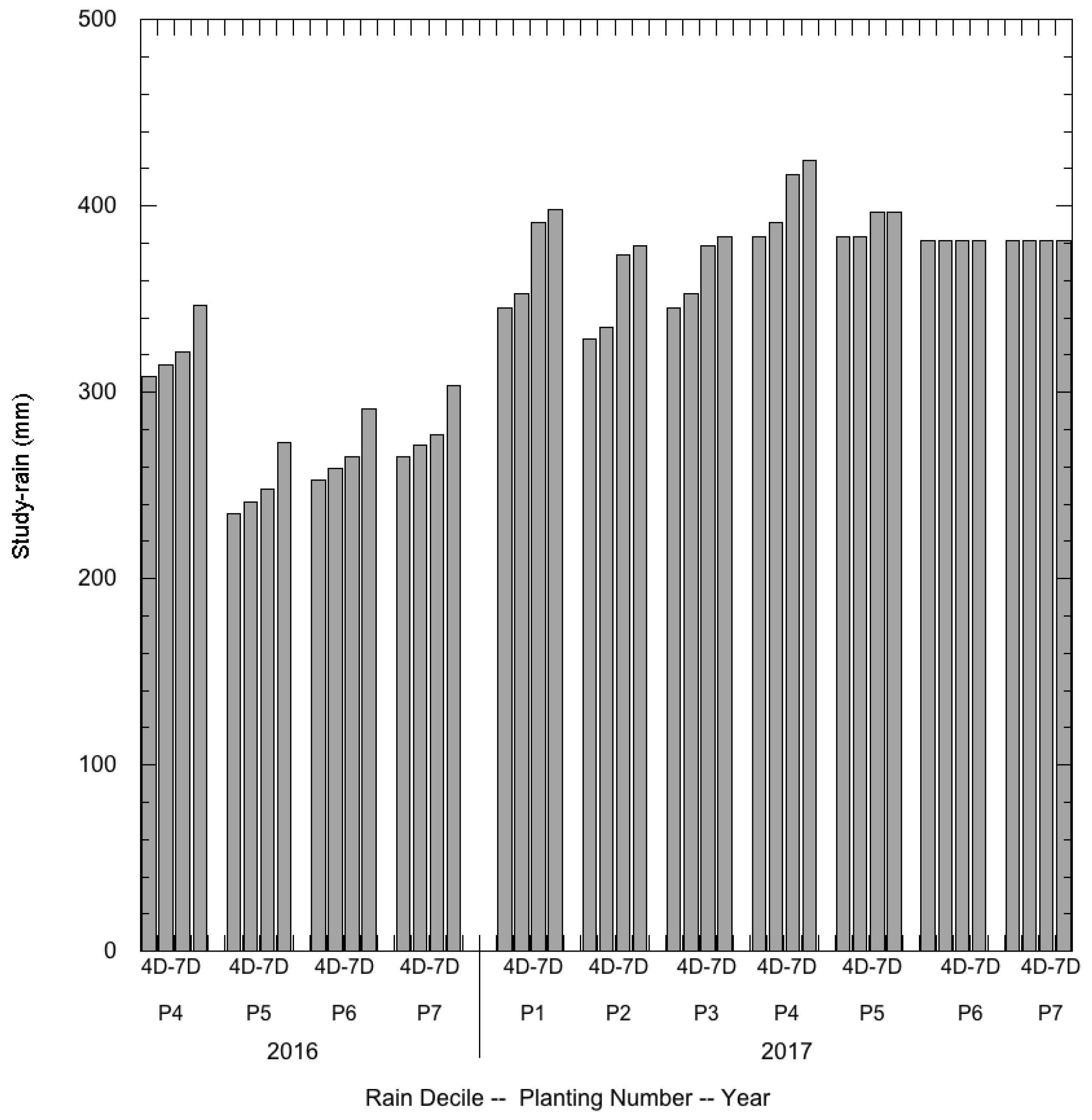
3.6. Rain across the Matrix Plantings

The study-rain on the matrix varied across rain simulations, planting dates, and years (Figure 7). The study-rain amounts were generally lower in 2016 than in 2017.

Table 3. Rain Outcomes shows an overview of the two years of the study. For brevity, the data shown is limited to the 4th decile of simulated rain all the planting dates.

Design	Lowest (mm)	Highest (mm)	Range (mm)	Matrix Rain Enhancement (mm)
Two Plantings	287	350	63	0
Eleven Plantings	215	350	135	72
Eleven Plantings with Four Rain Simulations	215	410	195	132

compares the two-year rain outcomes that would be achieved in three study designs. The two plantings represent the rain that would have been received on single planting (15 May) in each year. The 11 plantings represent the rain that would have been received on the 11 successful plantings in the two years. The 11 plantings with four rain simulations represent study-rain on the 11 successful plantings with rain simulations in the two years. The results indicate that study-rain across the two years varied from 215 to 410 mm. Across this 195 mm range, the inclusion of rain simulations increased the study-rain by 60 mm (17%) above the rain across the matrix. Compared to the single planting/year design, the planting matrix without rain simulations increased the range of rain by 72 mm and the inclusion of the rain simulations increased the range of rain by 132 mm. While the inclusion of rain simulations in 2016 and 2017 added to the rain variation, the extent of enhancement was limited by the volumes of rain received.

Given the above-average rain during 2016 and 2017, the rain exceeded the study-rain that was established in the 4th through 6th decile targets across all planting dates and exceeded the 7th decile targets in 33 of 44 water level plantings. The results underscore the limitations on a rain matrix when the rain amounts are above the range of study-rain defined by the treatment deciles. We chose to use the 4th through 7th deciles of rain as the treatment deciles in order to explore crop performance in the drier years as opposed to the wetter years of the rainfed environment. If rain in subsequent years of the matrix study is below normal we would anticipate a greater enhancement of study-rain to be produced. Regardless of the effectiveness of the rain simulations there was substantial variation in study-rain over the matrix (relative to the rain history of the region).

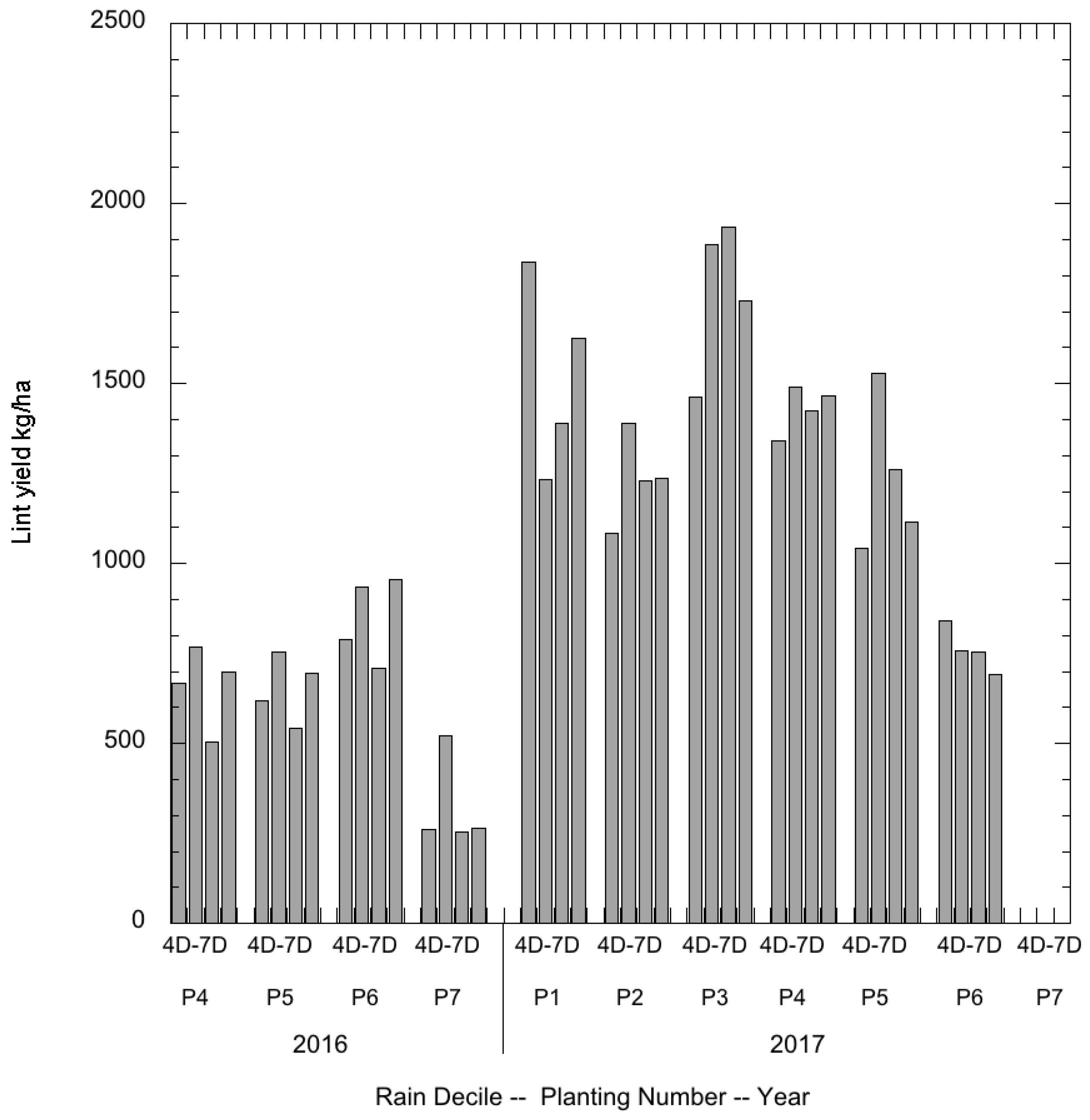
The yield for both years across the rain matrix treatments is shown in Figure 8. The yields in 2016 were lower across all treatments compared to 2017. The yield varied from 100 to 1900 kg/ha (planting 7, 4th decile in 2017 and planting 3, 6th decile in 2017). The extremely low yield in the 7th planting of 2017 is evidence of the planting not reaching maturity before the end-of-season freeze. Unlike the study-rain variation (Figure 7), there is no clear rain-decile effect evident.

Figure 9 shows that the relationship between study-rain and yield for the two years of the matrix study was relatively weak with an R²= 0.35. The goal of the rain matrix is to enhance the number of rain:yield pairs that can be generated in a single year and thus the absence of a strong rain:yield relationship is unexpected and troubling. The weakness of the relationship could be a result of a variety of factors that will be discussed in the following paragraphs.

The relationship between rain (water on the ground) and water used by the crop will affect the relationship between study-rain and yield. The concept of effective rain makes the distinction between rain that falls and rain that contributes to transpiration (the rain that makes yield). Only the fraction of rain that enters the plant and contributes to yield could be considered effective rain.

Under low water conditions of this study, the relationship between water on the ground (study-rain) and effective rain is potentially complex. Soil-related limitations in water availability become increasingly apparent as the water in the crop system declines. The fraction of water on the surface that enters the transpiration stream can be difficult to determine precisely. Under low-water rainfed conditions, soil variability can affect the availability of the water to the plant and thereby increase yield variability.

In addition to the effects of soil variability on the determination of effective rain amounts, the variability of the timing of rain events relative to the development of crop is potentially complex and significant [2]. Perhaps the inclusion of the temporal rain pattern would improve the study-rain versus yield relationship. In this analysis, we have focused on the study-rain amount as opposed to the patterns of study-rain which we intend to address at a later date.

Regardless of the relationship between study-rain and effective rain, the bias in this study would generally be toward an overestimation of water use based on the rain events. It is probably reasonable to assume that the weak relationship between yield and study water in the two years of the matrix study is, to an extent, a result of a difference between study-rain and effective rain.

3.7. The Role of Other Environmental Variables in Yield Relationships

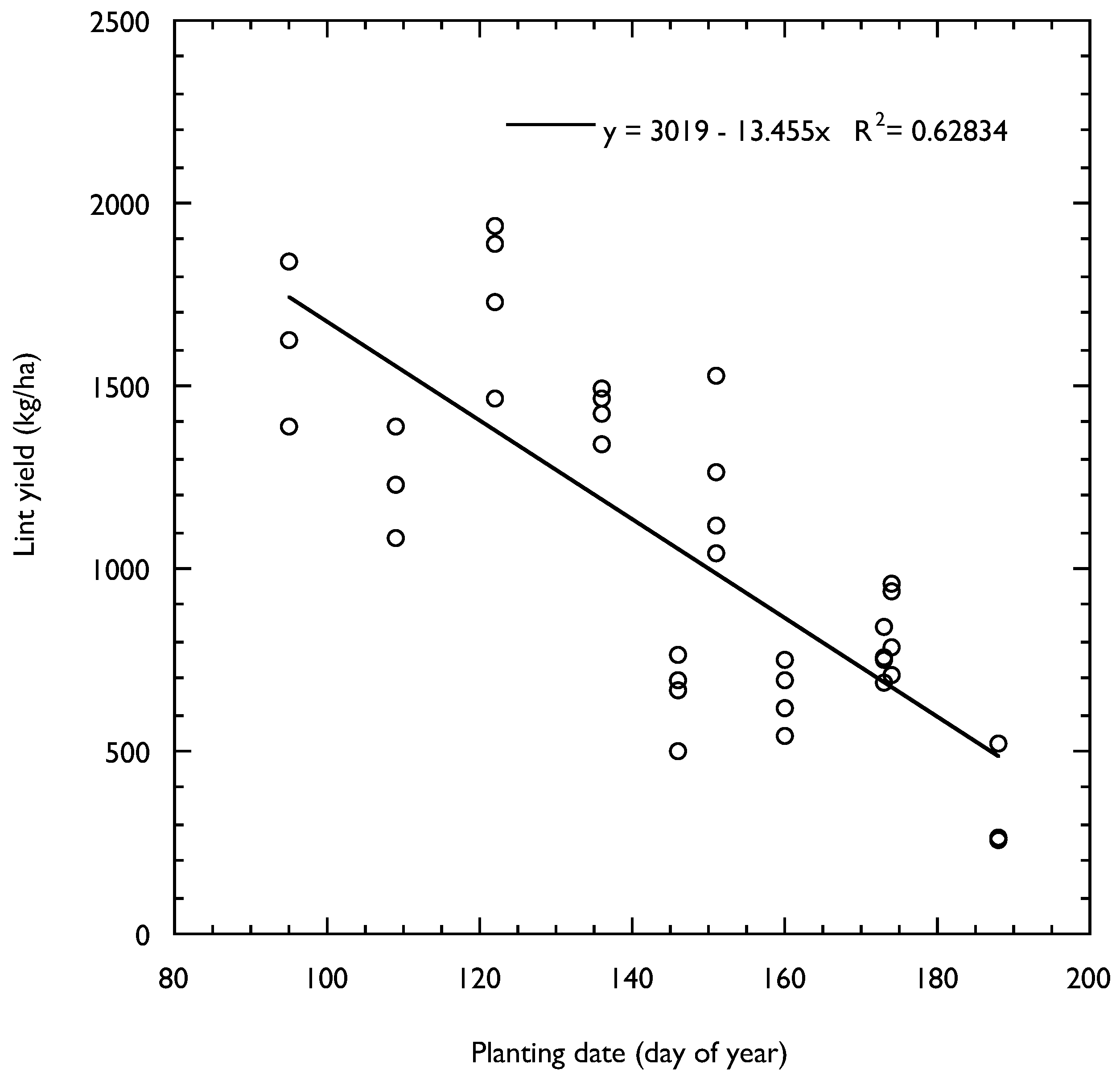
A goal of the study was to enhance the number of yield:rain pairs for cotton that could be produced in a single year. In addition to variation in study-rain, the sequential plantings used in the rain matrix result in a series of cotton crops that develop in different environments in terms of other important weather variables (e.g., temperature, humidity, solar radiation). Over the two-year study interval, the rain matrix resulted in a number of yield:environment pairs with differences in rain amounts. Thus, each entry in rain matrix results in a yield:environment pair with yield:rain pairs as a subset. The yield:environment pairs are represented by the relationship between planting dates (different crop environments) and yield (Figure 10). The relationship between planting date and yield was relatively strong (R² = 0.63) indicating that the putative environmental variability associated with planting dates contributed to variation in yield.

The differences in the strength of relationships of environment (planting date) and study-rain with yield suggest that other sources of environmental variation associated with the matrix affected yield to a greater extent than study-rain. Since sequential plantings are the basis of the rain matrix, the intermingling of effects of sources of environmental variation not associated with study-rain are a potential weakness inherent in the approach. The results from the two years of the study require us to consider the effects of non-water environmental variation on yield.

3.8. Temperature and Yield

Second only to water, temperature would generally be considered the most important environmental variable related to the performance of cotton at the study location. Given the relatively high altitude (975 m) and northern latitude (33°35’36”) of the Lubbock TX region, cotton production is generally considered to be limited by air temperatures during the growing season [11]. Given the thermal sensitivity of cotton production in the region, the various planting dates used in the rain matrix would be expected to introduce thermal variation that, while potentially important, is not directly related to rain.

Crop development and yield are generally related to the thermal environment such that, within a range of non-lethal temperatures, the rates of growth and development of crops increase with increasing temperature. Thermal environments in agriculture are often assessed in terms of heat units that have been shown to affect development and yield in a variety of crops. The accumulation of heat units is widely used in cotton for the scheduling of various management decisions (e.g., planting dates, irrigation timing, chemical applications) and rough in-season yield estimation. Heat unit accumulation over a growing season is generally sigmoidal with slow accumulation at the beginning and end of the season and the highest accumulation rates mid-season. The relationships among the rate of crop development, air temperature, and heat unit accumulation are empirical and dependent on a number of assumptions that have not been fully verified in low-water rainfed cotton systems [12,13]. In spite of potential limitations, heat unit accumulation provides a context for environmental temperature assessments.

3.9. The Accumulation of Heat Units for a Crop Begins at Planting and Ends with the Season

In order for a cotton crop in the region to reach maturity, the accumulation of at least 1250 heat units is generally considered necessary [14,15]. This 1250 heat unit value is widely accepted for the region and, since we used a commercial variety from the region, this 1250 heat unit requirement is perhaps a reasonable benchmark for comparing thermal environments. Heat unit accumulation relative to the 1250 value is often monitored as an indicator of progress toward crop maturity.

For each planting date, there are two ways that heat units can be counted. The first method calculates heat units on a calendar basis from planting to crop termination (a freeze or chemical application) and represents the heat units that are “available to the crop.” We will refer to these as “environment-heat units.” The second method is based on the development of the crop over the interval from planting to the date of crop maturity (60% open bolls). Since a cotton crop can reach maturity before crop termination, only those heat units between planting and maturity contribute to quality or yield. We will refer to these as “crop-heat units.” For each planting in the matrix, depending on the length of the period between crop maturity and crop termination (between 0 and 73 days in this study) the number of environment-heat units can be greater than or equal to the number of crop-heat units.

We have calculated environment-heat units and crop-heat units for the plantings in the study using a lethal freeze (air temperature <0 °C for 6 h) on November 20 as the date of season termination for both years of the study. Since heat unit accumulation among simulated-rain deciles was small (range <50 heat units), the heat units were calculated for each planting using only the 4th simulated-rain decile plots. Environment-heat units were calculated for all plantings in 2016 and 2017 based on the planting dates and the lethal-freeze date. Maturity dates, total water, and yield for plantings 1, 2 and 3 of 2016 could not be calculated as a result of a hailstorm in early June. While crop-heat units could be calculated only for plantings 4 through 7 in 2016, crop-heat units were calculated for all seven plantings in 2017.

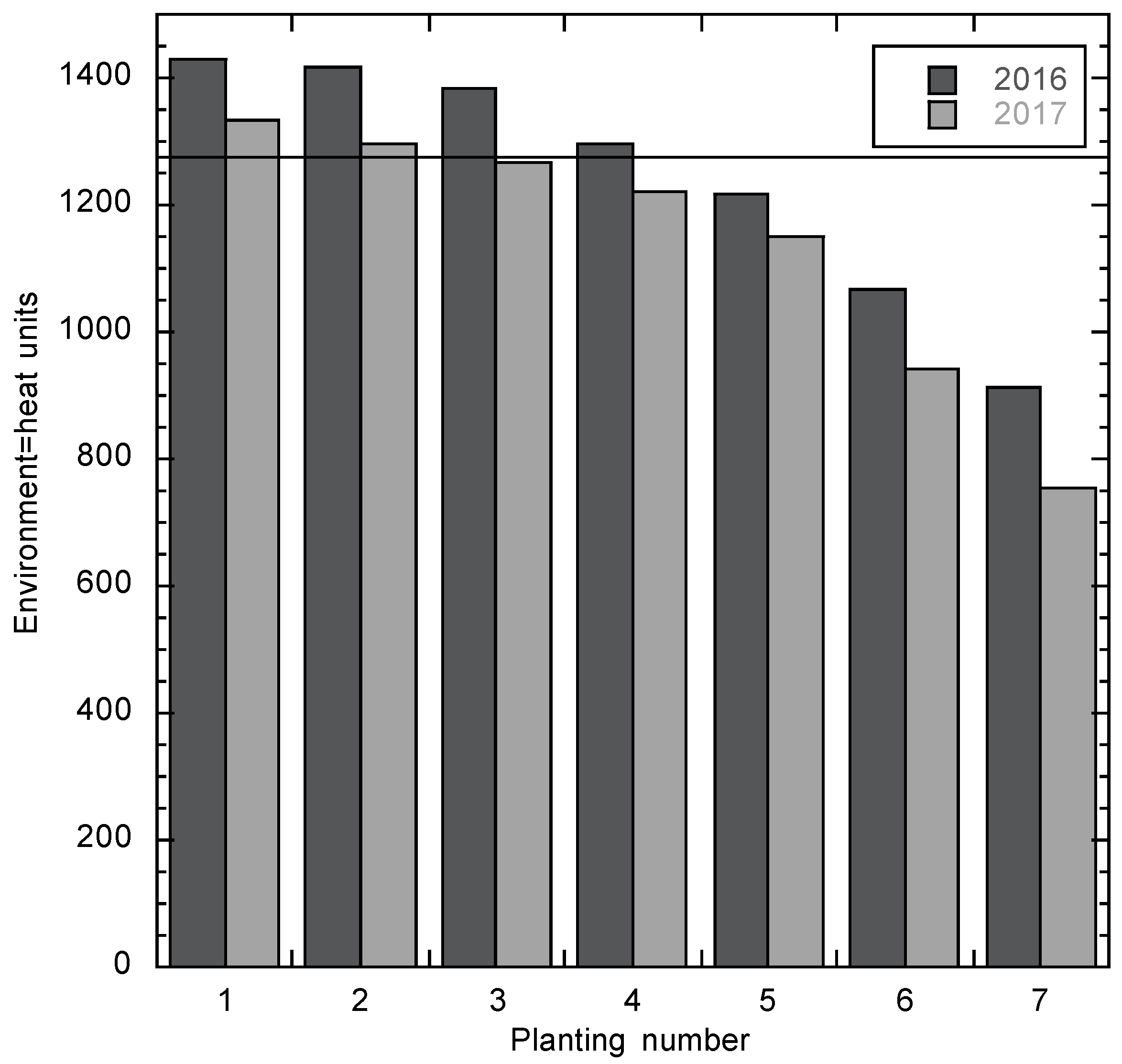
The number of environment-heat units varied with planting date in both years ranging from a maximum of 1428 in planting 1 of 2016, to a low of 753 in planting 7 of 2017 (Figure 11). For both years, there was a strong negative relationship (R² = 0.91) between the planting date and the environment-heat units. In general, 2016 had more environment-heat units than 2017 with environment-heat units across the seven planting dates varying from 913 to 1416 in 2016, and from 753 to 1331 in 2017. Environment-heat units were compared to the 1250 heat unit benchmark for maturity (Figure 11). In 2016, plantings 1 through 4 had at least 1250 environment-heat units available while plantings 5 through 7 fell short of the 1250 environment-heat unit value. In 2017 plantings 1 through 3 had at least 1250 environment-heat units available, while plantings 4 through 7 fell short of the 1250 environment-heat unit value as well.

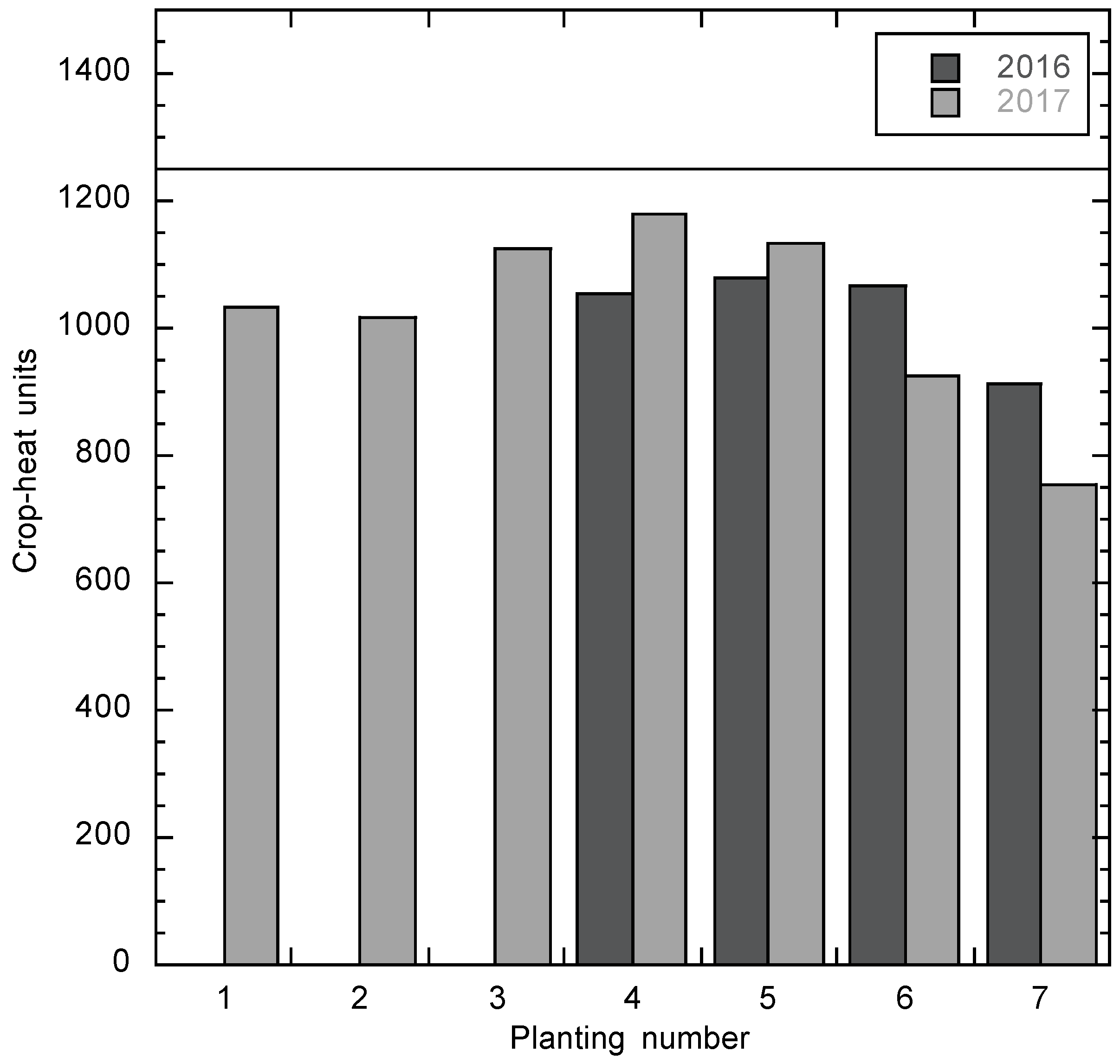
The number of crop-heat units over the course of the study varied in a manner similar to the environment-heat units ranging from a maximum of 1052 in planting 4 of 2016 to a low of 753 in planting 7 of 2017 (Figure 12). For both years, the relationship between the planting date and the crop-heat units was negative though relatively weak (R² = 0.56). In general, 2016 had more crop-heat units than 2017 with environment-heat units across the seven planting dates varying from 913 to 1053 in 2016 and from 753 to 1032 in 2017.

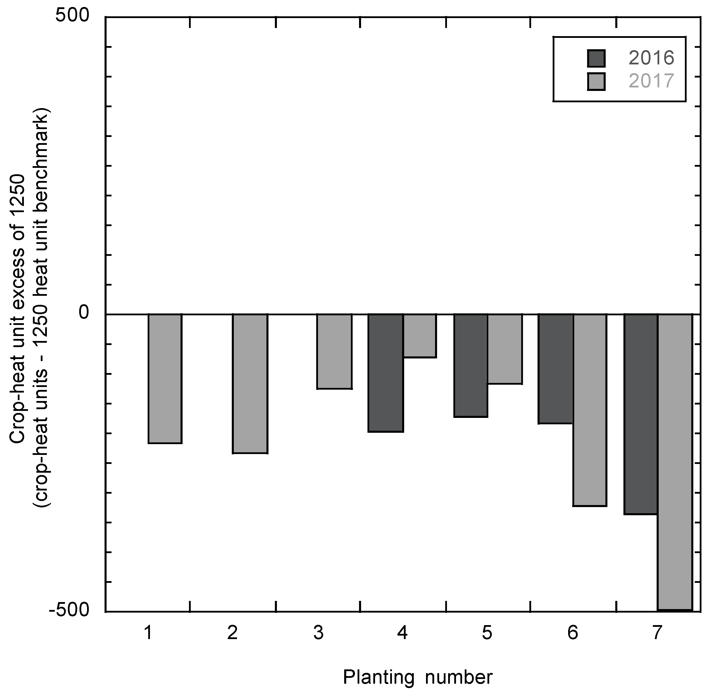
3.10. Crop-Heat Units versus Environment-Heat Units

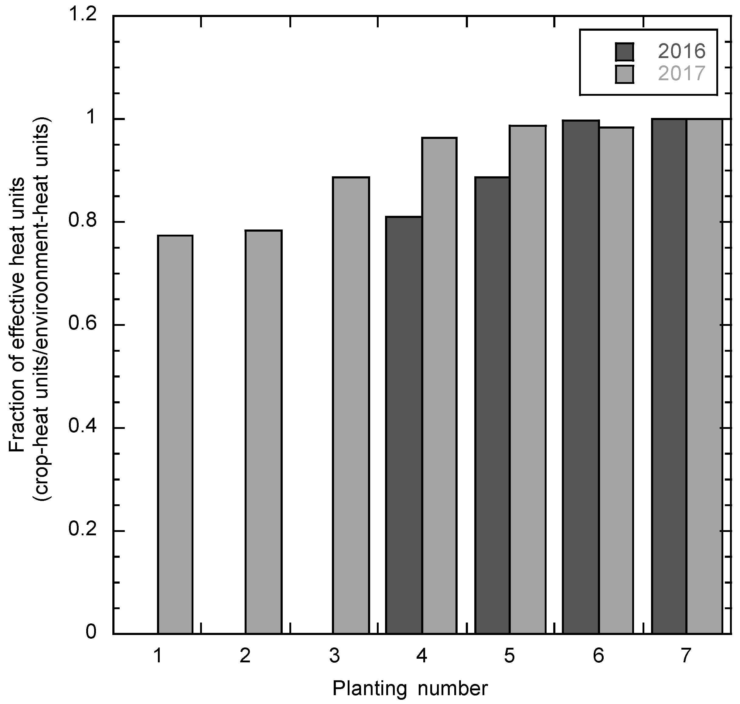
The difference between the environment-heat units and crop-heat units for the various plantings is shown in Figure 13. This number is potentially important since it indicates the fraction of environment-heat units that could have contributed to growth and development had the crop not reached maturity before the end-of-season freeze. Perhaps metric of “crop-heat units as a fraction of environment-heat units” could be seen as a measure of heat units that were available but not “used” by the crop. Crop-heat units as a fraction of environment-heat units indicates that in 2016, the crop-heat units comprised <90% of those available in plantings 4 and 5 (81% and 88%) while for plantings 6 and 7, the crop-heat units comprised 100% of those available. The pattern was similar in 2017 with crop-heat units comprising <90% of those available in plantings 1, 2, and 3 while plantings 4, 5, 6, and 7 the crop-heat units comprised 100% of those available. Out of the 11 plantings in the study, five could be considered to be not-limited in terms of available heat units (4 and 5 in 2016 and 1, 2, and 3 in 2017) and six were potentially limited by heat unit availability (6 and 7 in 2016 and 4, 5, 6 and 7 in 2017).

If indeed some plantings did not take advantage of the environment-heat units that were available, it is reasonable to ask if those plantings had already accumulated the 1250 heat units associated with maturity and were truly not thermally limited. In an effort to determine the extent to which some of the plantings might have indeed been limited with respect to heat units, the number of environment-heat units and crop-heat units was compared to the 1250 heat unit benchmark for maturity (Figure 14).

When environment-heat units were compared to the 1250 heat unit benchmark, plantings 1, 2 and 3 had more than 1250 heat units and were probably not heat unit limited between planting and lethal-freeze. Plantings 4 and 5 in both years were within 100 heat units of the 1250 value. Plantings 6 and 7 in both years had fewer than 1250 environment-heat units, falling short of 1250 by between 180 and 496 environment-heat units.

In terms of the crop-heat units versus the 1250 benchmark, none of the plantings in either year accumulated 1250 crop-heat units. The difference in effective heat units and the 1250 benchmark indicates a shortage between 70 and 496 heat units across the two-year matrix. This raises a question of how well the 1250 benchmark fits in the rainfed cotton in the two years of the study. Since even those plantings that had sufficient environment-heat units available reached maturity prior to reaching the 1250 value, a more appropriate benchmark value might be less than 1250. In terms of the number crop-heat units accumulated, the fact that all plantings achieved maturity (60% open bolls) without reaching the 1250 benchmark suggests that a more appropriate value might be as low as 900 heat units.

Regardless of the maturity threshold number, the heat unit-based analysis of the thermal environment indicates that, in addition to variation in total water across the matrix, there was thermal variation that could serve to complicate the relationships between rain and crop performance. Knowing that the thermal environment affects the outcomes provides the impetus for efforts to further understand the impacts and means to accommodate them in the experimental design.

3.11. Summary

We have described the design of a rain matrix experimental protocol and presented the results of two years of implementation. The two-year implementation of the rain matrix with a total of 14 cotton plantings across four rain simulation routines increased the magnitude of variation in water and yield compared to single planting designs.

It is fair to ask what advantages are offered by our rain matrix approach and is it worth the effort and complexity. We believe that the rain matrix that we have implemented is potentially useful because the combination of variation in natural rain and simulated rain provides the means to make more observations in a short time period than is afforded by non-matrix approaches.

As cotton can be relatively indeterminate in its growth habit, multiple planting dates have been used in many studies of environmental effects [16,17,18]. Many of these studies were focused primarily on the thermal environments associated with planting dates and were carried out under irrigated conditions that limited effects of rain variation. Davidonis et al. (2004) included both irrigated and rainfed treatments in their study with three planting dates to investigate fiber quality relationships. We are not aware of any previous field studies that have used a combination of planting dates and simulated rain to investigate rainfed cropping and believe that this approach may prove useful.

The relatively weak rain/yield relationships in the two years of the study indicate complicating factors that are not directly associated with seasonal rain amounts. The patterns of rain (which we did not analyze) may be significant in the rain:yield relationships and the analysis of rain patterns is currently underway. Though the relatively high rain amounts during the two years of the study limited the value of the rain simulations, rain matrix results in years with lower rain amounts will prove valuable. The relationships between yield and the thermal environments associated with the planting dates are not clear, though our heat unit analysis suggests they are potentially important as well. Even in the event that the yield, rain and thermal environment interactions are inseparable, the insights gained can provide information for the improvement of rainfed cotton production in the region.

We believe that the advantages associated with a rain matrix research design (e.g., a significantly increased number of yield:environment comparisons in a season) perhaps outweigh at least some of the weaknesses inherent in the approach (e.g., thermal variance, confounding by excessive seasonal rain). Regardless of the method employed, information in rainfed crop production will be necessary if we are to continue to provide food and fiber to a growing population in a world of diminishing water resources.

4. Conclusions

Rainfed crop production will undoubtedly increase in importance as expanding demand for food and fiber demand intersects with reductions in agriculturally exploitable land and declining water resources. Mitigation of yield reductions, if not increased production on rainfed lands, will become increasingly important in the future.

While the need for improved understanding of rainfed crop production systems becomes more urgent, the complexities inherent in rainfed research continue present an obstacle to the needed research. The development of improved rainfed production systems will require information on potentially complex interactions between the crop and the environment. Since weather and rain vary substantially within and among years, it is necessary to generate many comparisons of environment vs. crop performance.

In this study, we report the design and execution of a rainfed cropping research effort that is designed to increase the volume of information that can be generated in a single growing season. Initial results relating to a two-year implementation of a rainfed matrix experiment with cotton research on the southern high plains of Texas are reported. The system used a series of sequential plantings to allow the researcher to evaluate performance of cotton across and range of environments. Inclusion of a simulated-rain protocol creates an enhanced range of water and thermal environments within a single season.

The study was initiated in 2016 and the results for the first two years of the study, 2016 and 2017 were reported. A total of 56 combinations of plantings and water were established over the two years with 44 planting/water combinations resulting in harvestable yield. Though the two years were relatively wet for the region there was variation in rain across the matrix. As a result of the above average rain amounts, the amounts of the rain simulations were small (<18%) relative to the natural rain. Yield varied across the water/planting matrix though the relationship between study-rain and yield was relatively weak with an R² = 0.35.

The relatively weak relationship between crop water and yield underscores the complexities of the interactions among crops and their environments. While the total water varied across the matrix, the lack of a strong relationship suggests that (1) rain amounts and crop water use were not tightly connected. (2) The relationship between the total amount of rain and its effectiveness is a complex function of the amount and its timing relative to the crop. These relationships are perhaps worth studying. (3) Environmental variables other than rain varied across the matrix in a manner that reduced or masked the importance of water on the crop.

The fact that sequential plantings result in a variety of thermal environments across the matrix complicates, perhaps even negates, the contributions of a rain matrix system for understanding the water/yield relationships in cotton. This is not totally unexpected and results from additional years of study should help to understand not only rain but its interaction with other environmental factors in defining cotton production in a rainfed setting. The data from additional years of a rain matrix, with a broader range of natural rainfall and temperatures, may provide the basis for a more complete assessment of the utility of the approach.

A strength of a rain matrix design is that it is linearly scalable. While it can be implemented on a one-hectare field with a few varieties, it could also be readily expanded to screen a hundred varieties on 60 hectares. The goal of the rain matrix was to enhance the number of plant/environment response pairs that can be generated in a research setting. The multiple plantings and rain simulations over the two years produced a total of 44 plant/environment pairs, as compared with the two plant/environment pairs that would have resulted without the matrix design. In spite of the confounding elements of rain vs effective rain and variable thermal environments associated with the approach, we conclude that a rain matrix design might be useful in the study of rainfed cropping.