Article

Irrigation Analysis Based on Long-Term Weather Data

Cropping Systems Research Laboratory, USDA-ARS, 3810 4th Street, Lubbock, TX 79415, USA
*
Author to whom correspondence should be addressed.
Agriculture 2016, 6(3), 42; https://doi.org/10.3390/agriculture6030042
Submission received: 11 July 2016 / Revised: 18 August 2016 / Accepted: 22 August 2016 / Published: 31 August 2016
(This article belongs to the Special Issue Innovative Approaches to Agricultural Water Management)

Abstract

:
Irrigation management is based upon delivery of water to a crop in the correct amount and time, and the crop’s water need is determined by calculating evapotranspiration (ET) using weather data. In 1994, an ET-network was established in the Texas High Plains to manage irrigation on a regional scale. Though producers used the ET-network, by 2010 public access was discontinued. Why did producers allow a valuable irrigation-management tool to be eliminated? Our objective was to analyze the effect of declining well capacities on the usefulness of cotton ET (ETc) for irrigation. Thirty years (1975–2004) of daily ETc data were used to compare irrigation demand vs. irrigation responses at four locations, analyzed for multiple years and range of well capacities for three irrigation-intervals. Results indicated that when well capacities declined to the point that over-irrigation was not possible, the lower well capacities reduced the value of ETc in terms of the number of irrigations and total amount of water applied. At well capacities <1514 L·min−1 the fraction of irrigations for which ETc information was used to determine the irrigation amount was <35% across years and irrigation intervals. The value of an ETc-based irrigation may fall into disuse when irrigation-water supplies decline.

1. Introduction

The 1930’s drought that afflicted the Great Plains of the USA motivated the USDA in 1935 to start a weather forecasting program at Michigan Institute of Technology that became the foundation for the monthly weather forecasts distributed by the US Weather Bureau [1]. Furthermore, the drought compelled agricultural producers to irrigate crops, and questions of how much water and when to apply, i.e., irrigation scheduling, were asked. Attempts to answer these questions using weather networks were initially developed at the University of Nebraska in the early 1980’s [2]. Since then, the number of weather networks providing evapotranspiration (ET) estimates increased across North America. A survey in 1991 revealed 831 weather stations in USA and Canada [3], and in 1999, the number of weather stations had increased by 45% to 1200 [4]. Examples describing the technical aspects of the weather stations and of regional networks for different USA states are given for California [5], Ohio [6,7], Georgia [8], Oklahoma [9], Texas [10], and Washington [11]. This approach has also been used in other countries, e.g., Kenya [12], Australia [13], and Spain [14]. This is by no means an exhaustive list, and our purpose is to illustrate the proliferation and adoption of weather-generated information to provide estimates of the water requirements of crops. Our attention will focus on the current situation in the Texas High Plains (THP) in terms of the supply of irrigation water and adoption of the information generated by weather stations and used to determine estimates of crop ET.
In Texas, the history of irrigation is well documented [15,16]. It is known that in circa 1540, Native Americans had established irrigation systems near El Paso and Pecos, TX, USA, using water from the Rio Grande and Pecos River. Over a 28-year span, from 1716 to 1744, Franciscans were the first Europeans to irrigate crops using “acequias” (irrigation canals) in Catholic missions near San Antonio [17]. In Texas, corn (Zea mays L.) was the first field crop to be irrigated by both Native Americans and missionaries [16]. In the THP, large-scale irrigation started in 1920 and due to the scarcity of surface water, agricultural producers were forced to withdraw the groundwater, first with windmills and thereafter with irrigation pumps [18]. However, irrigation only became practical in the 1920–1930s with the development of the internal combustion engine [19] and also in response to the drought of the Dust Bowl [20]. The 1960’s were characterized as a decade of alarm due to the rapid decline of the ground water table [18].
The source of nearly all irrigation water in the THP is the Ogallala Aquifer [21], which is a large aquifer that covers eight states of the USA. In the THP, the Ogallala Aquifer is mostly a closed system where withdrawals exceed recharge, and over the years has resulted in a decline of the water table [19,21,22,23]. In some areas of the Ogallala Aquifer, this decline resulted in well capacities that produce less than the daily water requirements of crops, leading to the implementation of so-called deficit irrigation, i.e., the practice of applying less water than the water demand of the crop [24,25]. Also, and in response to this decline and to use seasonal rain, the sprinkler irrigation concept known as Low Energy Precision Application (LEPA) was developed for the THP [26,27,28]. This system was adapted for the declining well capacities of the THP that range from 1.3 to >7 mm·day−1 of the daily water supply [29]. The well capacity often determines the amount of water that can be applied regardless of environmental demand and crop needs. In some areas of the THP, the only irrigation option is to continuously water the crop throughout the growing season, from planting to harvest [29].
The development of irrigation systems such as LEPA [26,27] and sub-surface drip [30] requires an estimate of the daily water requirement of the crop. This value may be calculated by multiplying a potential or reference ET value by a crop coefficient (Kc), and this method is referred to as the “engineering approach” by [29]. This method was first suggested by [31] and is now the standard and recommended procedure for irrigation of crops worldwide [32,33]. This method to calculate ET provided a “standard” set of calculations for convenience and reproducibility for a hypothetical reference surface applied to a short and tall surface. The standardized reference evapotranspiration (ETsz) for a short crop (ETos) is a clipped and cool season grass (ETos) with a height of 0.12 m, and for a tall crop (ETrs), is full cover alfalfa with a height of 0.5 m [33]. The required weather inputs to calculate crop ETsz for either a short or tall crop are the same and include short-wave irradiance, air temperature and humidity, and wind-speed, normally measured at a screen-height of 2.0 m. An additional input is the surface soil heat flux. The availability of commercial weather stations with data-loggers able to record weather variables every second provide a range of timescales, from minutes to days, for the calculated values of crop ETsz for the entire growing season.
As previously described, the availability of commercial weather stations, advances in cellular communication and the Internet led to the development of “weather networks” that provided information on crop ETsz. In 1994, the Texas A&M University Research and Extension Service started the “South Plains Potential ET Network” with weather stations at Halfway, Lubbock and Lamesa, TX. The network provided daily values of ETsz and heat units from 1 April to 31 October, and the information was delivered on a daily basis via facsimile to subscribers that paid a nominal fee for the service. In 1995, a similar weather network was established in Amarillo, TX, i.e., “Texas North Plains PET Network” with weather stations at Dalhart, Etter, Morse, Whitedeer, Bushland and Dimmit [35]. Despite this expansion in coverage across the THP, fourteen years later in 2010, due to budget cuts and lack of support, public access to the weather networks was discontinued. This led us to question why irrigators and other users of the network allowed such a valuable tool to be eliminated from their operations in the THP. Perhaps it was reasonable to ask whether the usefulness of the system as an irrigation management tool was less than expected. Other relevant questions included did changes in irrigation and management practices over the life of the weather network reduce its value to the end users? To what extent do the irrigation recommendations of the ET network match the irrigators’ ability to act on those recommendations? While ET networks no doubt provide useful information on the magnitude and temporal pattern of ET over the course of a growing season, the extent to which such data can be considered “actionable” on the part of the irrigator is perhaps not fully understood or appreciated. Furthermore, our experience working with local producers, even those considered progressive irrigators, indicates that at least some remain unconvinced of the value and utility of the information delivered from ETsz networks.
We are not the first to question the value of weather networks to the end users as a tool for water management. The value of climate information as a decision making tool has been investigated [36,37,38,39], and the adoption of weather information has been reported [40,41,42]. In Texas, a survey sent to 900 agricultural producers indicated the importance of agricultural weather information, e.g., freeze warnings, precipitation probabilities, and soil temperature and water content, commonly broadcast over newspaper, TV and radio media; however, few producers were willing to pay for this information [43]. A similar conclusion was reached in Oklahoma where farmers and ranchers did not want to pay significant fees to have access to weather information beyond raw data [44]. Nevertheless, technology transfer of agricultural water management programs from weather networks via extension and outreach activities remains a high priority in Nebraska [45] and elsewhere. The occurrence of drought events remains a driver for the use and adoption of “smart” irrigation controllers based on ET [46] and in the adoption of information generated from weather networks. For example, in California, users of the California Irrigation Management Information System increased over a 5-year span (1986 to 1991) from 500 to 2000 [47].
To provide insight and to answer the previous questions, we selected and used 30-year (1975–2004) weather data sets for four locations of the THP to investigate the relationship between ET-based irrigation recommendations for cotton (Gossypium hirsutum L.) and the ability of irrigators to manage irrigation with those recommendations. While our research approach is specific to our location, climate and crop, we believe that our method has general applications to other regions and crops. Our goal was to identify options to improve the successful adoption of ET-based irrigation as a management tool [45,48]. Our purpose is not to evaluate specific advantages or disadvantages of any particular irrigation system for cotton production in the THP. Furthermore, we present a first “order solution” to address the decline in irrigation water, and we do not consider the many agronomic options that are available, e.g., capture of rain, cotton varieties, crop rotations, minimum tillage, and other practices that are in use in the THP. The increased competition for water between agriculture and urban users [49] and the continued incidence of droughts gives us renewed interest in improving tools that irrigators could use to manage water efficiently.

2. Materials and Methods

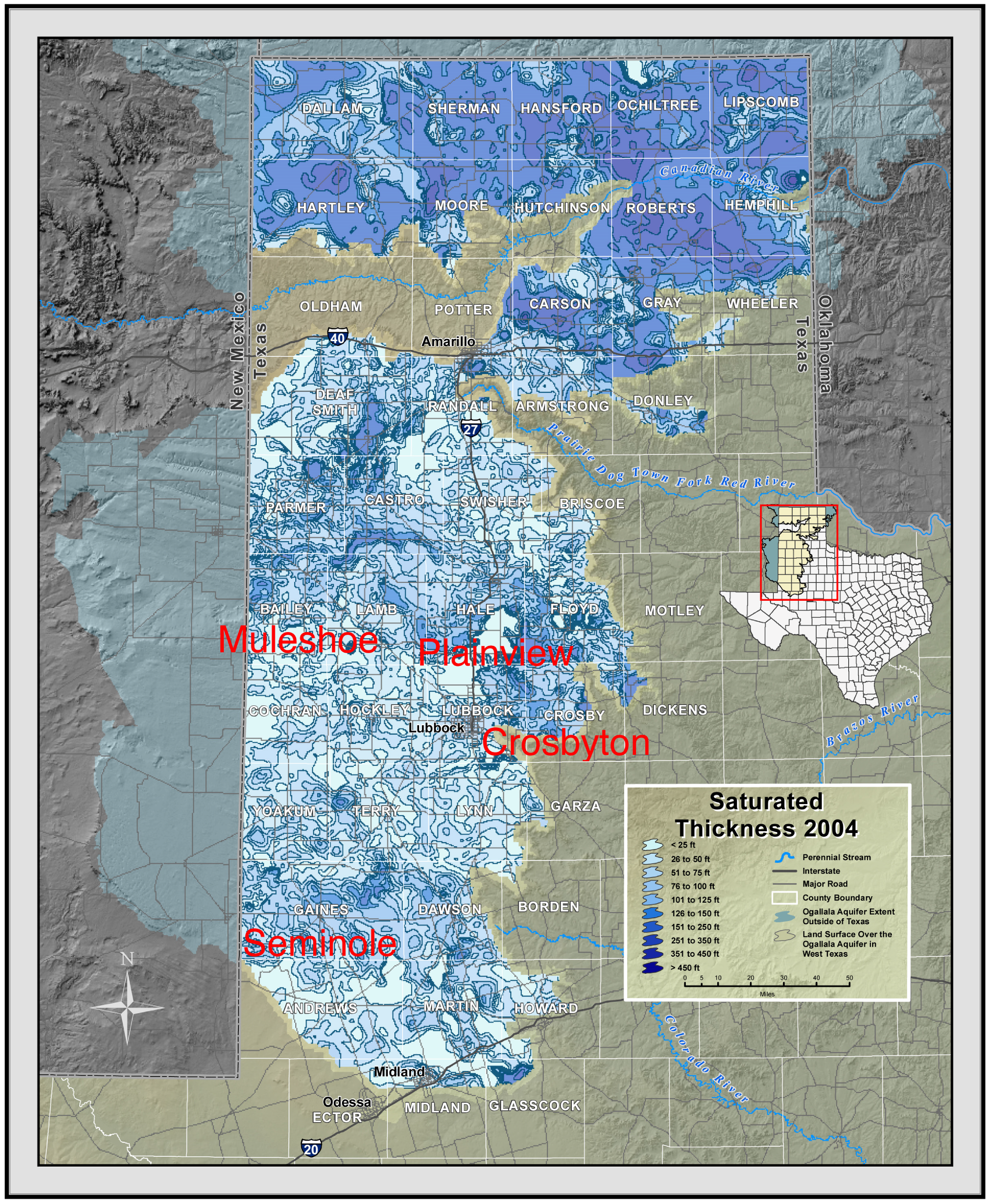
2.1. Study Area and Irrigation Practices

The study area consisted of four sites across the THP, Muleshoe (Bailey County), Seminole (Gaines County), Crosbyton (Crosby County) and Plainview (Hale County). Irrigation well capacities within the THP range from 1.3 to 7.6 mm·day−1 [26,29], and the saturated thickness of the Ogallala Aquifer ranges from <15 m to >180 m (Figure 1).

2.2. Usefulness of an ET-Based Irrigation Management System

One way to assess the usefulness of an ET-based irrigation management system is to measure the extent to which availability of the ET information generated by the management system influences the irrigator’s decisions. Such an assessment of ET-based irrigation compares the irrigation demand calculated from crop ET and the irrigation response of the irrigator to that demand. Ultimately, the usefulness of any ET-based irrigation management system depends on the strength of the linkage between irrigation demand and irrigation response. Our approach was to calculate pairs of irrigation demand and irrigation response amounts over a period of years, for various irrigation systems, and to determine how the demand and response amounts were affected.
In a well-functioning irrigation management system, in the absence of limitations in irrigation water, the irrigation response would equal the irrigation demand and, as water becomes limiting, the irrigation response amounts would decrease relative to the irrigation demands. Limitations in irrigation water are typically a result of two factors: (1) well capacity, the specific quantity of water that a well will yield per unit of time, e.g., L·min−1 [50,51]; and (2) irrigation-interval, i.e., the number of days between irrigation events. For example, in a center pivot, this is determined by the speed of the pivot. Well capacity is subject to change over time given the thickness and properties of the water-bearing strata and depth to ground water. The irrigation interval is related to several factors, e.g., irrigation method, soil type and crop.
Cotton is a perennial plant grown as an annual that is well adapted to arid climates and responds well to frequent deficit irrigation at different intervals and thus is well-suited to a variety of irrigation methods. The two main irrigation methods used in the THP are center pivots (~400 m long) and subsurface drip, and for both methods, the irrigation strategies are designed to use seasonal rain and irrigation water efficiently [26,27,28]. We selected three time-intervals (1, 5 and 10 days) and five well capacities (1.3, 2.5, 4.1, 5.1, and 7.6 mm·day−1) associated with an irrigated area of 41 ha. Thus, the irrigation methods, irrigation intervals and well capacities represent irrigation practices common in the THP. For example, for the selected irrigation intervals, a sub-surface drip irrigation system could be operated on any of the three time-intervals, while the 5-day and 10-day are perhaps more representative of center pivot irrigation systems. The selection of an irrigation interval involves aspects of crop water use, soil characteristics and irrigation equipment. Sub-surface drip can often be implemented at 1-day intervals though under some conditions (limited water or in-season rain), extension to a 5-day interval can be advantageous in terms of enhanced root development. In center pivot systems, increasing the amount of irrigation water applied per event by increasing the irrigation interval can reduce soil water evaporation associated with such systems. In general, the trend in the THP has been towards increasing the irrigation interval. Further, a 10-day irrigation interval may be unusual, but in sandy soils, might be beneficial. A summary of the well capacity and irrigation interval used in our analysis is given in Table 1.

2.3. Calculation of Cotton ET (ETc)

We used the standardized reference equation for a short crop (ETos) [33] using as input 30 years (1975–2004) of daily weather data for Muleshoe, Seminole, Crosbyton, and Plainview (Figure 1). These daily ETos values were calculated using the Ogallala Agro-Climate Tool given by [52]. The daily reference ETos values for each location were then used to calculate corresponding daily values of cotton ET (ETc) in mm·day−1, as adjusted by a crop coefficient (Kc) given by [32] as follows:
E T C = E T O S × K C
Daily values of ETc were calculated for a 110-day period from 15 May (Day Of Year, DOY 135) to 31 August (DOY 243) for each 30-year interval (Figure 2a). This 110-day period represents the average length of a cotton-growing season where the cotton crop would be irrigated.

2.4. Calculation of Irrigation Demand

Irrigation demand (mm of water) was calculated from the ETc values (Equation (1)) described above and by grouping ETc values into three classes: (1) 1-day sums; (2) 5-day sums; and (3) 10-day sums, resulting in 143 irrigation demand values for each year at each of the four sites over the 30-year period. Since this procedure generated a total of 17,160 irrigation demand values, we limited our analysis to Plainview, TX, USA, where we conducted previous studies [53]. Further, using the 30-year interval at Plainview generated 4290 irrigation demand values, and we limited the analysis by segregating the data into five groups consisting of: (1) 1988, the lowest total ETc year; (2 and 3) 1981 and 2001, moderate total ETc years; (4) 1980, the highest total ETc year; and (5) the 30-year mean of ETc for the 110-day period (Figure 2b). Thereafter, and for the 110-day irrigation period, we summed the daily values of ETc for the three daily irrigation intervals (1-, 5- and 10-day) as follows:
j d a y = i   =   1 1   =   110 E T c , i
where j is the time interval in days, i.e., 1-day, 5-day and 10-day, and i is the value of ETc (mm) for each day of the 110-day period. These calculations yielded 110 values for the 1-day, 22 values for the 5-day, and 11 values for the 10-day interval, for a total of 143 values of ETc for each of the five groupings for a total of 715 irrigation demand values. Each ETc value represents an irrigation demand (mm of water) based on calculated values of ETc.

2.5. Calculation of Irrigation Response

In our analysis, irrigation demand is an irrigation goal that the irrigator may or may not be able to meet, and the irrigation response represents the amount of irrigation water (mm) that the irrigator is able to apply in response to the demand. The assessment of the usefulness of the ETc-based irrigation method involves calculating irrigation responses for each of the 715 calculated irrigation demands at each of the five well capacities. The irrigation response associated with each irrigation demand is primarily determined/limited by the amount of water that can be applied in response to the demand. For each of the 715 calculated irrigation demand values, an irrigation response amount (mm) was calculated for each of the five well capacities that define the limits on the irrigation response (Table 1). For the three irrigation intervals and five well capacities, the following decision criteria were applied to produce irrigation demand/irrigation response pairs for possible irrigation events:
If   irrigation   demand   maximum   irrigation ,   then Irrigation   response   =   irrigation   demand
and
If   irrigation   demand >   maximum   irrigation ,   then Irrigation   response   =   maximum   irrigation
Applying this approach of using ETc for the irrigation of a cotton crop in Plainview, over four representative years and the 30-year mean at three irrigation intervals and the five well capacities (Table 1), resulted in 3575 irrigation scenarios for analysis.

2.6. Analysis of Irrigation Demand/Irrigation Response Pair Usefulness

Based on the above criteria, the usefulness of an irrigation demand/irrigation response pair was assessed in terms of the extent to which the irrigator’s decision was affected by the ETc-based information. Two irrigation outcomes were possible, first as defined in Equation (3), when (1) irrigation demand ≤ maximum irrigation, the irrigator applies an irrigation that matches the irrigation demand and thus has altered irrigation in response to the ETc-based value (ETc was useful). This is defined as “variable-amount irrigation”. Second, as defined in Equation (4); when (2) irrigation demand > maximum irrigation, the irrigator applies an irrigation amount equal to the maximum irrigation capacity of the system, and thus the irrigation applied was not altered in response to the ETc-based value (ETc was not useful). This ETc–independent irrigation is defined as “maximum-amount irrigation”.
The usefulness of the ETc-based approach over a season was determined by the fraction of seasonal irrigations that were variable-amount irrigations. The amount of water applied in maximum-amount irrigations is defined by well capacity instead of ETc. It is proposed that the usefulness of ETc-based irrigation methods declines as the fraction of variable-amount irrigations declines. Each of the 3575 irrigation demand/irrigation response pairs was categorized as a variable-amount irrigation or maximum-amount irrigation in accordance with the preceding criteria.

3. Results and Discussion

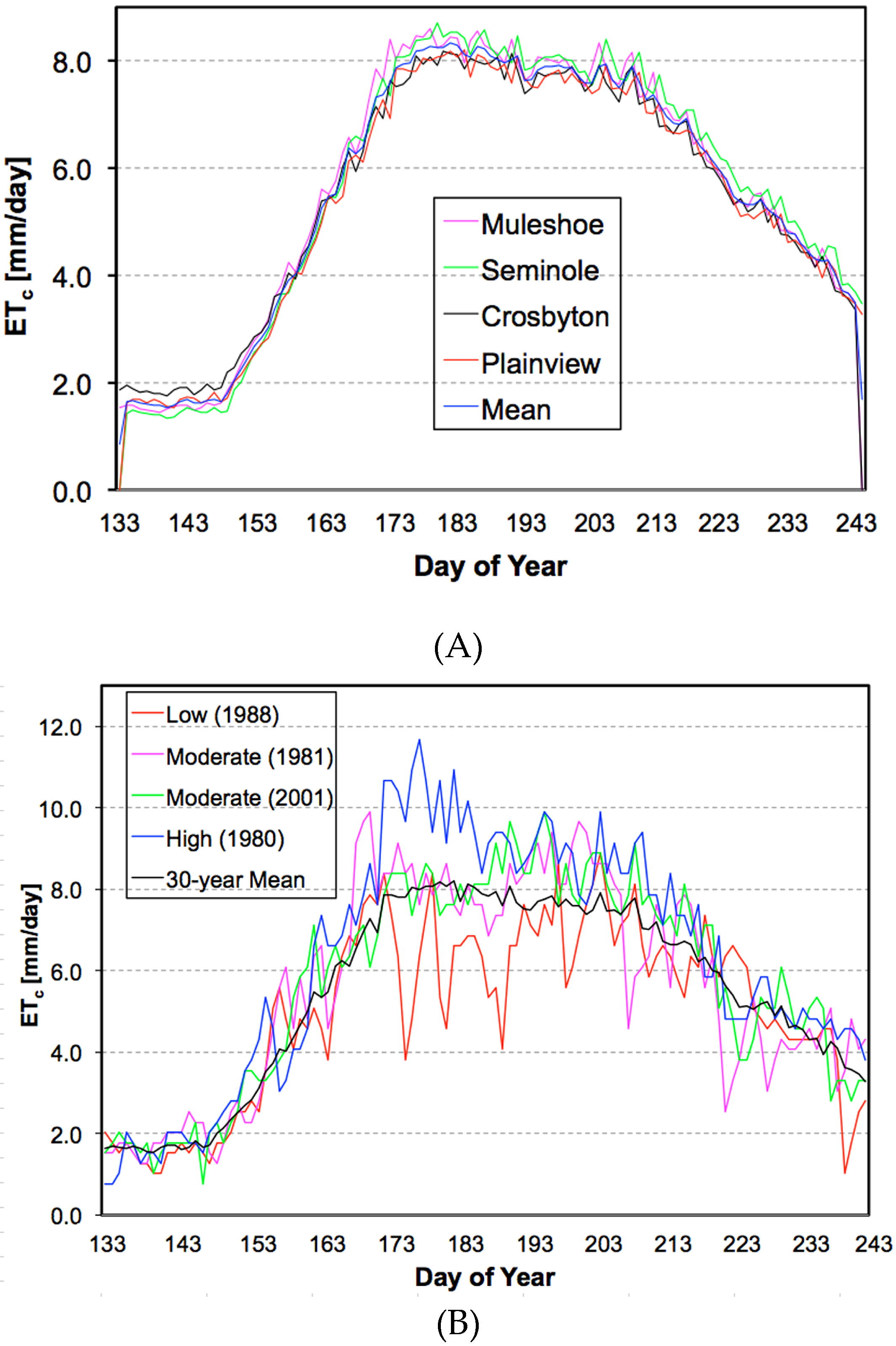
3.1. Seasonal ETc Patterns for the 30-Year Period

Statistical analysis of the 30-year ETc data for the four sites indicated similar values for the mean (5.5), median (6.0), standard error (SE = 0.23), and coefficient of variation (CV = 43%) (Table 2). The mode was similar for Muleshoe and Crosbyton (~7.9), and for Seminole and Plainview (~1.5). The skewness was negative, about −0.5 at all four sites, indicating that the ETc data were slightly skewed left. The kurtosis was also negative, about −1.1 at all four sites, indicating a heavy-tailed distribution [54]. The Shapiro-Wilk test for normality yielded a value of 0.9 for the four sites (p-value 1.9 × 10⁻⁷). The similarity of these results is not surprising given that the four selected sites are within 200 km of each other (Figure 1), even though they delineate a large region that is irrigated in Texas [55].

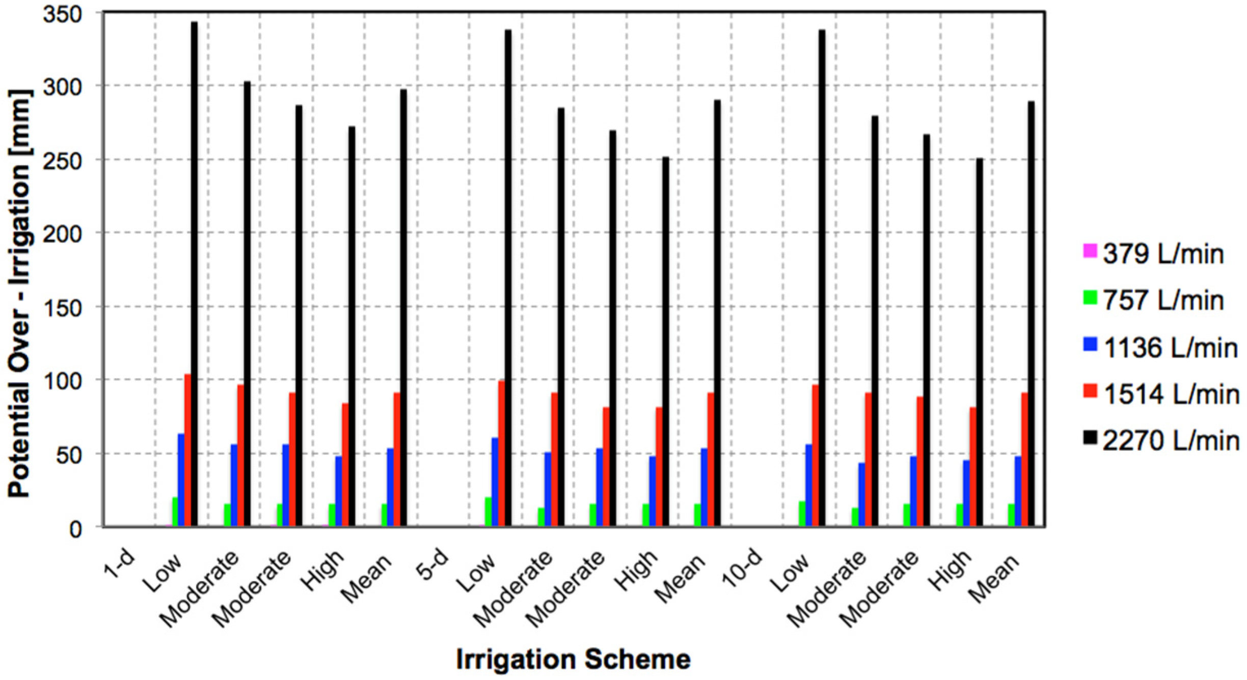
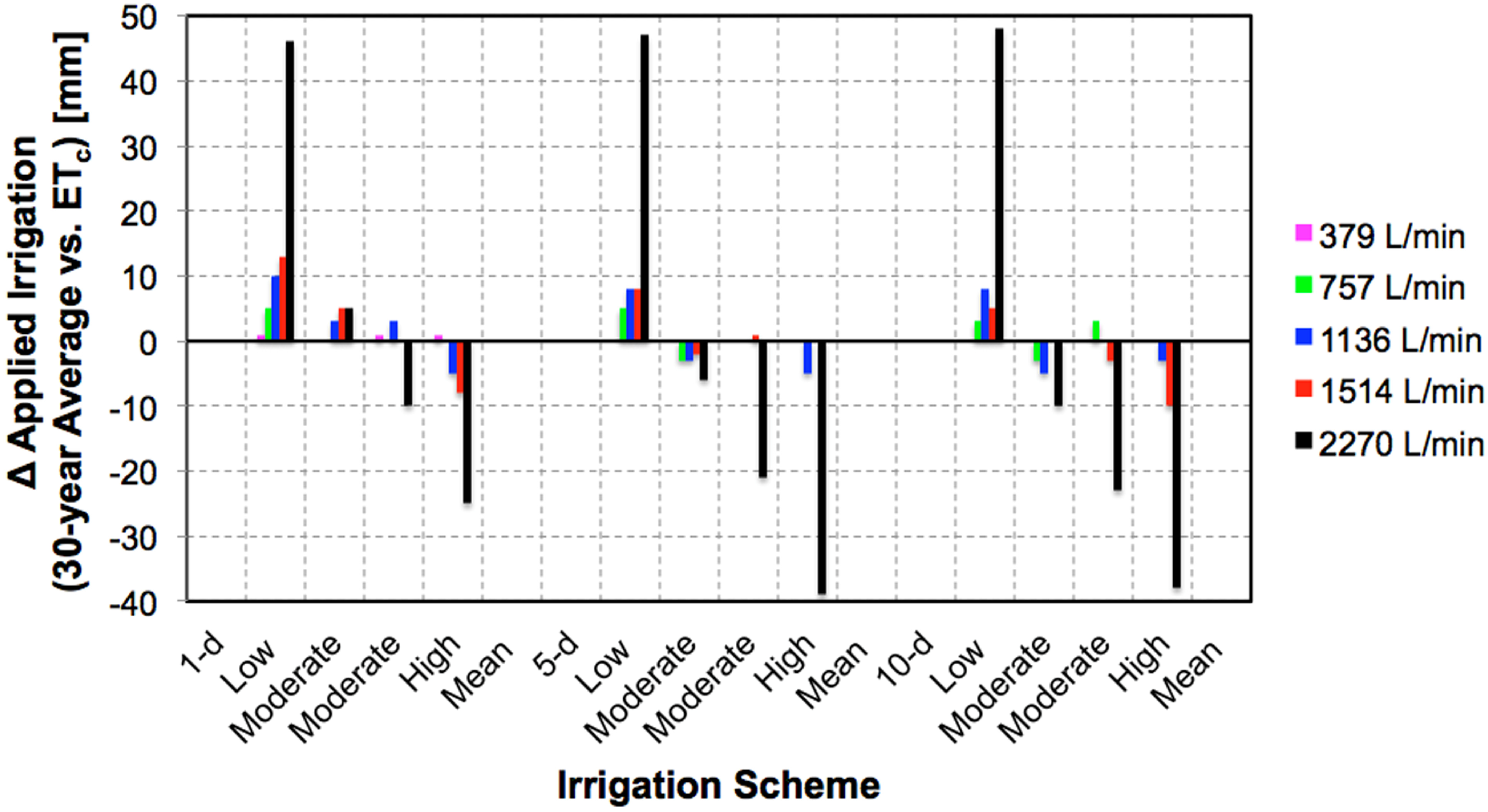
3.2. Role of ETc-Based Irrigation to Prevent Over-irrigation

A potentially significant advantage of using an ETc-based irrigation scheme is the prevention of over-irrigation as compared to irrigation schemes that are based on applying predetermined periodic irrigation with a fixed amount of water, e.g., 50 mm every 5 days. In a typical “available amount” or “maximum-amount” scenario, an irrigator would apply the maximum amount of water that is available, i.e., well capacity, in each irrigation event. This approach is often used in regions where water is abundant and/or inexpensive as was the case in the early years of irrigation in the THP [21,22].
In a maximum-amount irrigation scenario, the amount of irrigation applied over the 110-day irrigation period, as used in this study, equals the maximum daily irrigation amount multiplied by 110. This amount is unaffected by weather conditions and is only a function of the well capacity. For the well capacities used in this study, the seasonal maximum-amount of irrigation applied would be 143 mm for the 379 L·min−1 well capacity, 275 mm for the 757 L·min−1, 451 mm for the 1136 L·min−1, 561 mm for the 1514 L·min−1, and 836 mm for the 2270 L·min−1. With respect to the potential to over-irrigate, the amount of over-irrigation in a season at each well capacity depends on the cumulative ETc over the 110-day period and thus is related to the specific year and location. The amount of over-irrigation associated with a given seasonal ETc amount is the difference between the maximum amount and the ETc amount for the same period.
The calculated seasonal (110-day) ETc for Plainview, TX, USA, was 551 mm for the low ETc year (1988), 618 and 629 mm for the two moderate ETc years (1981 and 2001), 687 mm for the high ETc year (1980), and 599 mm for the 30-year mean. For example, the potential of over-irrigation for the 2270 L·min−1 well capacity would be the difference between 836 mm and 551 mm, i.e., 285 mm for the low ETc year, 281 mm and 207 mm for the two moderate ETc years, 149 mm for the high ETc year, and 237 mm for the 30-year ETc mean. Over-irrigation amounts for the five well capacities, over four years and the 30-year period, are shown in Figure 3. The results show that, in all years of the analysis, the potential for over-irrigation decreased as the well capacity decreased. At the lowest well capacity (379 L·min−1) it was not possible to over-irrigate, whereas for the 1-day irrigation interval at the highest well capacity (2270 L·min−1), the minimum and maximum over-irrigation amounts for the high ETc year were 270 mm and 345 mm, respectively. Over-irrigation of >300 mm occurred in the low ETc year regardless of irrigation frequency (Figure 3). These results indicated that a crop-based ET system provides the opportunity to reduce the amount of irrigation applied for well capacities >1000 L·min−1, though the water saved declined as the total seasonal irrigation decreased. These over-irrigation outcomes represent an upper limit, as rainfall is not included in this evaluation. However, in practice, in regions with low rainfall, many irrigators with sufficient water resources often ignore in-season rain in their irrigation management strategies. In essence, irrigators will ignore the efficiency of irrigation in order to achieve the crop yield stability that is associated with excess irrigation. A maximum irrigation amount strategy is primarily an economic objective as opposed to an agronomic management decision. All else being equal, there are clear advantages to implement an ETc-based irrigation when over-irrigation is a possibility and represents an obvious first step in water conservation when over-irrigation, while possible, is no longer a desired outcome.

3.3. Usefulness of ETc-Based Irrigation in the Absence of Over-irrigation

One goal of this study was to explain why the ETc-network on the THP fell into disuse. Clearly on farms where over-irrigation is possible, but not considered a problem, adoption of an ETc-based approach would not be expected, and the suspension of the region’s ETc-network might go unnoticed by producers. As the ability of producers in the THP to over-irrigate has largely disappeared over the past 20 years, what other factors might have contributed to a reduction in the perceived value of an ETc-based management? The ability to tailor irrigation amounts to match variation in crop water demand is a foundational aspect of ETc-based irrigation and the basis of its usefulness for producers. However, the ability to vary the irrigation response relative to the irrigation demand decreases in synchrony with declining water availability. The value of the ability to alter the irrigation response relative to ETc-based irrigation demand may be characterized in terms of frequency and the total amount of water associated with its occurrence. Previously, the irrigation response was broadly categorized into variable-amount (ETc dependent) and maximum-amount (ETc independent) irrigations with the usefulness of using ETc decreasing as the fraction of maximum-amount irrigations increased.

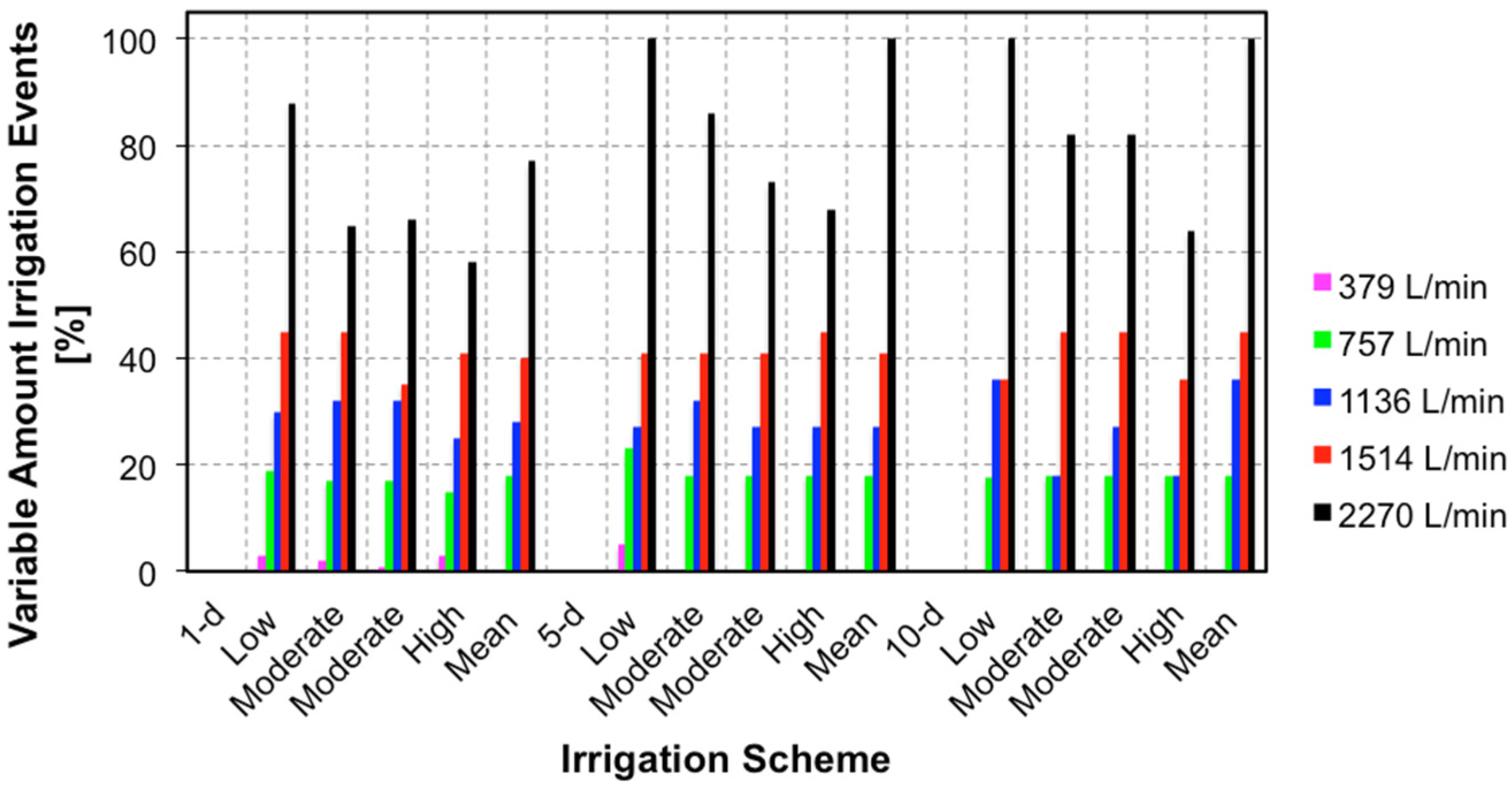
3.4. Frequency of Variable-Amount Irrigations Events

The variable-amount irrigation events as a function of well capacity and the five irrigation schemes are shown in Figure 4. The fraction of variable-amount irrigation events was influenced by well capacity and less so by years and irrigation intervals. For the lowest well capacity (379 L·min−1), the percent of variable-amount irrigation events was low and varied between 0 and 3% for all irrigation schemes. For the highest well capacity (2270 L·min−1), the percent of variable-amount irrigation events was higher, with 100% of irrigation events categorized as variable-amount irrigations for the low ETc year (1988) and the 30-year ETc average for the 5-day and 10-day irrigation intervals. In general, for all the irrigation intervals and well capacities, variable-amount irrigations were <20% for the two lowest well capacities (379 and 757 L·min−1). Variable-amount irrigation events were generally between 30% and 45% for the 1136 L·min−1 and 1514 L·min−1 well capacities. At the highest well capacity (2270 L·min−1), variable-amount irrigation events ranged from 58% to 100%. The results showed that as well capacities declined, as they have on the THP, the irrigator’s ability to alter irrigation amounts in response to ETc information declines. Regardless of the year or irrigation interval, when well capacity <1514 L·min−1, the fraction of irrigations that can be modified by ETc information is <50%. As the well capacity further declines, the usefulness of the ETc information provided by the network commensurately also declines. How an irrigator responds to this decline in actionable information is unknown, but it possibly contributes to a reduction in the perceived value of the weather network.

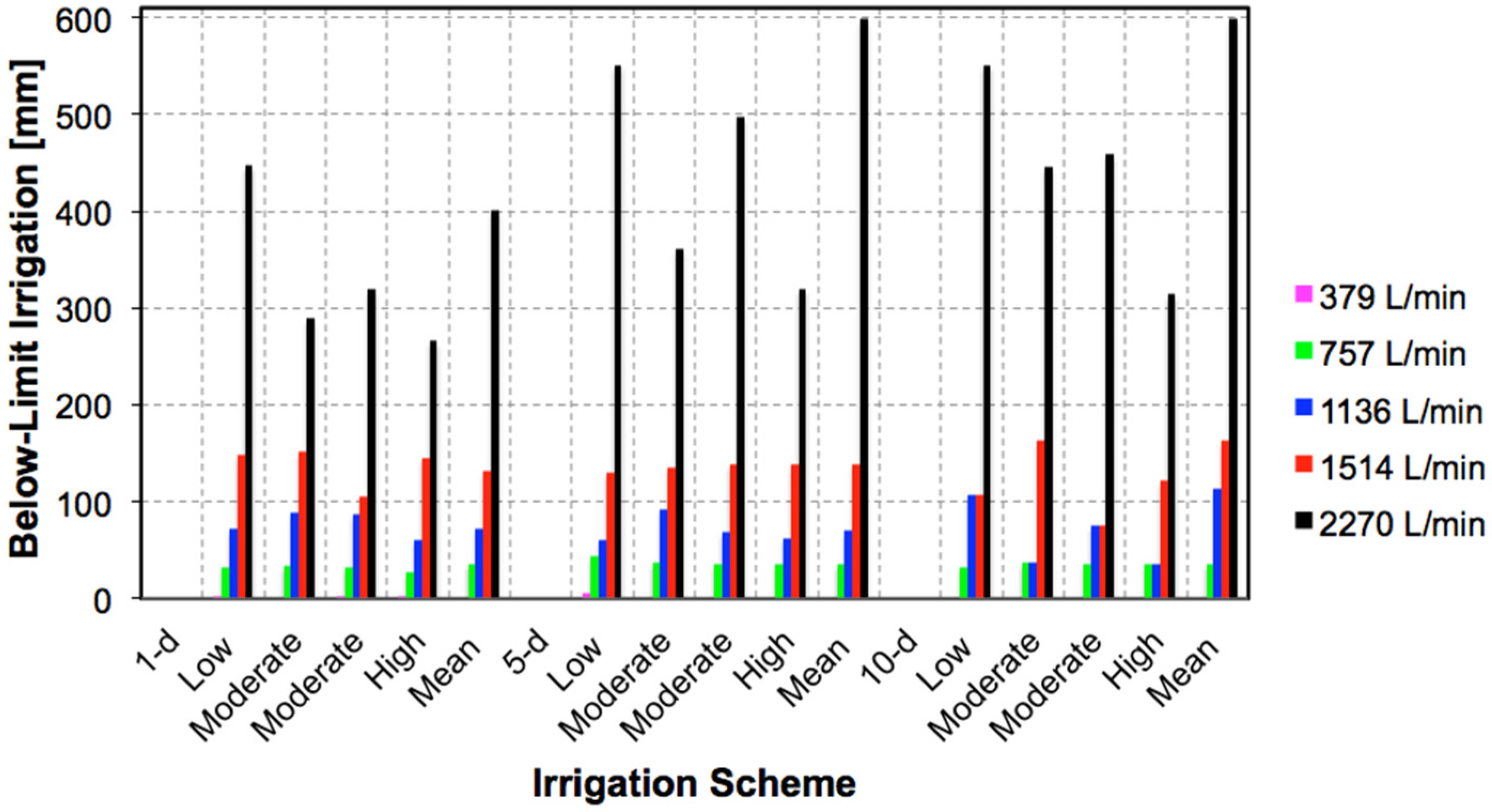
3.5. Amounts of Water Associated with Variable-Amount Irrigations

While the fraction of variable-amount irrigations declined with declining well capacity, the amount of water associated with those irrigations also declined. While the fraction of useful ETc measurements might be 50%, the amount of water involved may decline to the point that it becomes unimportant from the irrigator’s point of view. The seasonal amount of water applied when the calculated value of ETc resulted in applications not limited by the well capacity, i.e., variable-amount irrigation, is shown in Figure 5. These examples illustrate situations where the use of calculated values of ETc resulted in water savings as compared to simply irrigating at the maximum-amount (well capacity). Figure 5 shows the seasonal irrigation applied in variable-amount irrigations for all irrigation schemes and well capacities. As expected, the amounts of water applied in variable-amount irrigations were: <6 mm at 379 L·min−1, <44 mm at 757 L·min−1, <112 mm at 1136 L·min−1, <164 mm at 1514 L·min−1 and <598 mm at 2270 L·min−1 (Figure 5). Thus, the total amount of water that was “saved” using the ETc method declined with declines in well capacity, perhaps further diminishing the perceived value of ETc.

3.6. Reduced Usefulness of ETc-Based Irrigation at Low Well Capacities

As the irrigation capacity declined, the potential for over-irrigation decreased, and the usefulness of an ETc-based approach for the prevention of over-irrigation is limited. In the absence of over-irrigation, the primary value of an ETc-based system lies in the extent to which it allows the irrigator to match the irrigation response (amount applied) to variation in the irrigation demand (ETc amount). These results demonstrated that in the THP, as well capacities decline below 2270 L·min−1 the usefulness of an ETc-based irrigation management is diminished from the irrigator’s point of view. Based on these results, at well capacities ≤1514 L·min−1, the fraction of variable-amount irrigation events (Figure 4) and the amount of water associated with such irrigations (Figure 5) declined both in absolute and in relative terms. At the lower well capacities, the irrigation strategy often becomes one in which the goal is to apply the maximum amount of water possible at the shortest interval allowed by the irrigation system [29,53]. Under these conditions, the relevance of scheduling irrigation based on ETc declines.
In the THP, the producer’s lack of interest in ETc information provided by the ET network from 1994 to 2010 might be partially explained by the declining well capacities. Furthermore, surveys have indicated that agricultural producers in Texas and Oklahoma are not willing to pay for weather information beyond raw data [43,44], and these are factors that contribute to the challenges in maintaining an operational ET network that producers may use for water management.

3.7. Value of Historic vs. Real-Time ETc Values in Irrigation Management

In the THP, the apparent decline in the usefulness of using ETc-based irrigation management for many, but not all, producers, raises the question, “to what extent can historic long-term values of ETc be used in place of real-time ETc data supplied by weather networks?”
The usefulness of using historic ETc instead of real-time daily values of ETc supplied by weather networks was compared using 30-year average daily values of ETc. The difference in applied irrigation when using the 30-year average ETc minus the “real-time” value of daily ETc provided by a weather network as a function of well capacity for the four years (low ETc, 1988, moderate ETc, 1981 and 2001, and high ETc, 1980) at Plainview, TX, USA, is shown in Figure 6. The difference in irrigation amount varied among irrigation intervals and well capacities. For example, at the high well capacity (2270 L·min−1), using the long-term average ETc resulted in an over-irrigation of about +50 mm in the low ETc year across all irrigation frequencies. Also, at the high well capacity using the 30-year average resulted in under-irrigation of about −40 mm in the high ETc year for the 5-day and 10-day irrigation intervals. The equivalent amount of under-irrigation for the 1-day irrigation interval was −25 mm (Figure 6). For all other years, well capacities and irrigation intervals, the differences in irrigation amounts applied between the long-term (30-year) average and “real-time” were on average similar, i.e., −1 ± 6 mm. A potential problem when using a 30-year average value of ETc is that in years when ETc is low, over-irrigation could occur, and similarly in years with high ETc, under-irrigation could occur. The practical significance of this bias would have to be viewed in light of the possible value of implementing ETc-based irrigation in a region where there is minimal support to implement a real-time ETc network. These results suggested that in the THP, the potential water savings from using a “real-time” value of ETc compared to the 30-year average are, for practical purposes, minimal. This result suggest that ETc based irrigation can reduce both over- and under-irrigation.

4. Conclusions

The results presented are best described in terms of an irrigation management approach based on a simple water balance, i.e., inputs and outputs. The primary input factor is the amount of irrigation water that can be applied over the growing season of the crop. This input is adjusted according to the rainfall received and amount of stored soil water. Given these inputs (irrigation, rain and stored soil water), how much water does the crop need and when should this water be applied? In our example, we selected and used a demand-response irrigation approach to answer these questions.
The results showed that when irrigation resources are sufficient for over-irrigation, a crop-ET approach provides the means to prevent over-irrigation, and the implementation of crop-ET approaches will generally result in reducing the amount of irrigation water applied. Further, when irrigation water is not limiting, differences in irrigation water applied when using a “real-time” daily ETc compared to a 30-year average ETc are minimal. This result suggested that it is reasonable to implement an ETc-based irrigation using long-term values of ETc, wherever “real-time” ETc is not available. In our example, for the THP using a 30-year average ETc for irrigation of cotton crop for a range of well capacities and irrigation schemes compared to a daily value of ETc from a weather network, resulted in similar values of irrigation water applied. Further, these differences are within the application “error” that can be achieved with sprinkler and drip irrigation systems. This finding suggests that even in the absence of a real-time weather network to generate ETc values, the use of a long-term historic ETc table by an irrigator is useful to reduce over-irrigation and perhaps to generate interest in the establishment of a real-time ETc network.
An initial question posed in our study was “why does it appear that irrigators in the THP are not making full use of ETc-based irrigation management?” Weather network ETc-based systems were introduced to the study area in the mid-1990, when well capacities where in the 2270 L·min−1 range (Wagner, 2012). However, over the past two decades irrigation capacities have significantly declined, and irrigation goals have shifted from preventing over-irrigation to deficit irrigation. Our results showed that, when well capacities decline to <2270 L·min−1, the usefulness of an ETc-based irrigation management declines to the extent that the perceived value of the weather network becomes less apparent and perhaps effectively non-existent from the irrigator’s perspective.
One additional explanation for the decline in the use of public ET networks is the possibility that producer’s lack of participation may be a result of them using private on-farm weather stations to calculate ET. Advances in weather monitoring make this a real possibility and may indeed contribute to the possible loss of interest in public networks. In this instance, loss of participation could be seen as an indicator of the producer’s perceived value of ET-based scheduling as opposed to a lack of interest. Such an analysis is beyond the scope of this paper but might be valuable in some instances.
What are the broader implications of these findings? The transition from an irrigation management designed to prevent over-irrigation to a deficit-irrigation approach is occurring in many irrigated regions. On the THP where this study was conducted, a combination of reduced well capacities and governmental regulation of water withdrawals have resulted in response limits on irrigation that may require the development of non-ETc based irrigation management.
It is perhaps worth asking, why did the producers simply reduce the irrigated area to accommodate the reduced water supply? Currently, in the THP, there is interest in approaches to reduce irrigated areas in an economically advantageous manner. During the early 2000’s, the issue was possibly complicated by the introduction of cotton varieties with increased water productivity that to some extent offset lint yield losses due to declining irrigation. Finally, insurance issues associated with the shift from irrigated to rainfed may have created some obstacles to abandonment of irrigated area that were not based solely on agronomic considerations. Again, this transition is now occurring in the THP, and efforts to reestablish the regional ET network are underway.
Current research in the ET irrigation community is focused on improving the coverage of weather networks with improved methods to calculate crop ET [56,57]. In addition, there is great interest and parallel effort directed toward the development of improved crop coefficients, e.g., [58,59,60]. Regardless of these efforts, it is probable that improvements in ET delivery and crop coefficients will not be sufficient to overcome the limits on ETc-based irrigation management that result from declining water resources. Our results suggest that the inclusion of an irrigation management analysis based on a demand-response concept may prove useful to assess the utility of irrigation management schemes in general and with regard to research aimed toward improving or refining a given approach. When an ETc-based irrigation management is to be implemented/refined, it might be helpful to ask the question; how will this improvement/refinement affect how the irrigator will respond to an irrigation demand? While increasingly local and accurate demand values may be obtainable, their value to the irrigator may be ultimately inconsequential.

Acknowledgments

This research was supported in part by the Ogallala Aquifer Program, a consortium between USDA-Agricultural Research Service, Kansas State University, Texas A&M AgriLife Research, Texas A&M AgriLife Extension Service, Texas Tech University, and West Texas A&M University.

Author Contributions

Both authors equally contributed to data analysis and the writing of the manuscript. James Mahan was responsible for the initial idea of questioning the value of weather networks for water management in areas where water resources are declining.

Conflicts of Interest

The authors declare no conflict of interest. Mention of trade names or commercial products in this publication is solely for the purpose of providing specific information and does not imply recommendation or endorsement by the U.S. Department of Agriculture. USDA is an equal opportunity provider and employer.

Abbreviations

CVcoefficient of variation
DOYday of year
ETcrop evapotranspiration (mm·day−1)
ETccotton ET (mm·day−1)
ETszstandardized reference ET (mm·day−1)
ETosETsz for a short crop (mm·day−1)
ETrsETsz for a tall crop (mm·day−1)
Kccrop coefficient
LEPAlow energy precision application
SEstandard error
THPTexas High Plains

References

  1. Hecht, A.D. Drought in the Great Plains: History of societal response. J. Clim. Appl. Meteorol. 1983, 22, 51–56. [Google Scholar] [CrossRef]
  2. Changnon, S.A.; Lamb, P.J.; Hubbard, K.G. Regional climate centers: New institutions for climate service and climate-impact research. Bull. Am. Meteorol. Soc. 1990, 71, 527–537. [Google Scholar] [CrossRef]
  3. Meyer, S.J.; Hubbard, K.G. Nonfederal automated weather stations and networks in the United States and Canada: A preliminary survey. Bull. Am. Meteorol. Soc. 1992, 73, 449–457. [Google Scholar] [CrossRef]
  4. Elliott, R.L.; Hubbard, K.G.; Brusberg, M.D.; Hattendorf, M.J.; Howell, T.A.; Marek, T.H.; Snyder, R.L. The role of automated weather networks in providing evapotranspiration estimates. In National Irrigation Symposium, Proceedings of the 4th Decennial Symposium, Phoenix, AZ, USA, 14–16 November 2000; pp. 243–250.
  5. Howell, T.A.; Meek, D.W.; Phene, C.J.; Davis, K.R.; McCormick, R.L. Automated weather data collection for research on irrigation scheduling. Trans. ASAE 1984, 27, 386–391. [Google Scholar] [CrossRef]
  6. Curry, R.B.; Klink, J.C.; Holman, J.R.; Elwell, D.L.; Sciarini, M.J. Current Ohio experience with an automated weather station network. Appl. Eng. Agric. 1988, 4, 150–155. [Google Scholar] [CrossRef]
  7. Elwell, D.L.; Klink, J.C.; Holman, J.R.; Sciarini, M.J. Ongoing experience with Ohio’s automatic weather station network. Appl. Eng. Agric. 1993, 9, 437–441. [Google Scholar] [CrossRef]
  8. Hoogenboom, G. The Georgia automated environmental monitoring network. In Proceedings of the 1993 Georgia Water Resources Conference, Athens, GA, USA, 20–21 April 1993; Hatcher, K.J., Ed.; Institute of Natural Resources: Concord, CA, USA, 1993; pp. 398–402. [Google Scholar]
  9. Brock, F.V.; Crawford, K.C.; Elliott, R.L.; Cupercus, G.W.; Stadler, S.J.; Johnson, H.L.; Eilts, M.D. The Oklahoma Mesonet: A technical overview. J. Atmos. Ocean. Technol. 1995, 12, 5–19. [Google Scholar] [CrossRef]
  10. Schroeder, J.L.; Burgett, W.S.; Haynie, K.B.; Sonmez, I.; Swirka, G.D.; Doggett, A.L.; Lipe, J.W. The West Texas Mesonet: A technical overview. J. Atmos. Ocean. Technol. 2005, 22, 211–222. [Google Scholar] [CrossRef]
  11. Pierce, F.J.; Elliott, T.V. Regional and on-farm wireless sensor networks for agricultural systems in eastern Washington. Comput. Electron. Agric. 2008, 61, 32–43. [Google Scholar] [CrossRef]
  12. Stewart, J.I.; Hash, C.T. Impact of weather analysis on agricultural production and planning decisions for the semiarid areas of Kenya. J. Appl. Meteorol. 1982, 21, 477–494. [Google Scholar] [CrossRef]
  13. Zhang, Y.; Leuning, R.; Chiew, F.H.S.; Wang, E.; Zhang, L.; Liu, C.; Sun, F.; Peel, M.C.; Shen, Y.; Jung, M. Decadal trends in evaporation from global energy and water balances. J. Hydrometeorol. 2012, 13, 379–391. [Google Scholar] [CrossRef]
  14. Vanderlinden, K.; Giráldez, J.V.; Meirvenne, M.V. Assessing reference evapotranspiration by the Hargreaves method in Southern Spain. J. Irrig. Drain. Eng. 2004, 130, 184–191. [Google Scholar] [CrossRef]
  15. Arneson, E.P. Early irrigation in Texas. Southwest. Hist. Q. 1921, 25, 121–130. [Google Scholar]
  16. Bloodworth, M.E.; Gillett, P.T. IRRIGATION—Handbook of Texas Online; Texas State Historical Association: Austin, TX, USA, 1984; Available online: http://www.tshaonline.org/handbook/online/articles/ahi01 (accessed on 20 June 2016).
  17. Hutchins, W.A. The community acequia: Its origin and development. Southwest. Hist. Q. 1928, 31, 261–284. [Google Scholar]
  18. Green, D.E. Land of the Underground Rain: Irrigation on the Texas High Plains, 1910–1970; University of Texas Press: Austin, TX, USA, 1973; p. 326. [Google Scholar]
  19. Musick, J.T.; Pringle, F.B.; Walker, J.J. Sprinkler and furrow irrigation trends: Texas High Plains. Appl. Eng. Agric. 1988, 4, 46–52. [Google Scholar] [CrossRef]
  20. Opie, J. Ogallala—Water for a Dry Land, 2nd ed.; University of Nebraska Press: Lincoln, NE, USA, 2000; p. 475. [Google Scholar]
  21. Colaizzi, P.D.; Gowda, P.H.; Marek, T.H.; Porter, D.O. Irrigation in the Texas High Plains: A brief history and potential reductions in demand. Irrig. Drain. 2009, 58, 257–274. [Google Scholar] [CrossRef]
  22. Musick, J.T.; Pringle, F.B.; Harman, W.L.; Stewart, B.A. Long-term irrigation trends: Texas High Plains. Appl. Eng. Agric. 1990, 6, 717–724. [Google Scholar] [CrossRef]
  23. Scanlon, B.R.; Faunt, C.C.; Longuevergne, L.; Reedy, R.C.; Alley, W.M.; McGuire, V.L.; McMahon, P.B. Groundwater depletion and sustainability of irrigation in the US High Plains and Central Valley. Proc. Natl. Acad. Sci. USA 2012, 109, 9320–9325. [Google Scholar] [CrossRef] [PubMed] [Green Version]
  24. English, M.J.; Musick, J.T.; Murty, V.V.N. Deficit irrigation. In Management of Farm Irrigation Systems; Hoffman, G.J., Howell, T.A., Solomon, K.H., Eds.; American Society of Agricultural Engineers: Saint Joseph, MI, USA, 1990; pp. 631–663. [Google Scholar]
  25. Fereres, E.; Soriano, M.A. Deficit irrigation for reducing agricultural water use. J. Exp. Bot. 2007, 58, 147–159. [Google Scholar] [CrossRef] [PubMed]
  26. Lyle, W.M.; Bordovsky, J.P. Low energy precision application (LEPA) irrigation system. Trans. ASAE 1981, 24, 1241–1245. [Google Scholar] [CrossRef]
  27. Lyle, W.M.; Bordovsky, J.P. LEPA irrigation system evaluation. Trans. ASAE 1983, 26, 776–781. [Google Scholar] [CrossRef]
  28. Bordovsky, J.P.; Lyle, W.M.; Lascano, R.J.; Upchurch, D.R. Cotton irrigation management with LEPA systems. Trans. ASAE 1992, 35, 879–884. [Google Scholar] [CrossRef]
  29. Lascano, R.J. A general system to measure and calculate daily crop water use. Agron. J. 2000, 92, 821–832. [Google Scholar] [CrossRef]
  30. Camp, C.R. Subsurface drip irrigation: A review. Trans. ASABE 1998, 41, 1353–1367. [Google Scholar] [CrossRef]
  31. Jensen, M.E. Water consumption by agricultural plants. In Water Deficits in Plant Growth; Kozlowski, T.T., Ed.; Academic Press: New York, NY, USA, 1968; Volume II, pp. 1–22. [Google Scholar]
  32. Allen, R.G.; Pereira, L.S.; Raes, D.; Smith, M. FAO—Irrigation and Drainage Paper, No. 56, Crop Evapotranspiration; FAO—Food and Agriculture Organization of the United Nations: Rome, Italy, 1998; p. 326. [Google Scholar]
  33. Allen, R.G.; Walter, I.A.; Elliott, R.; Howell, T.A.; Itenfisu, D.; Jensen, M.E. The ASCE Standardized Reference Evapotranspiration Equation; ASCE-EWRI Task Committee Report; American Society of Civil Engineers: Reston, VA, USA, 2005. [Google Scholar]
  34. Saturated Thickness 2004. Available online: http://www.depts.ttu.edu/geospatial/center/Ogallala/MapSeries/PDFs/03_SatThickness_8x11.pdf (accessed on 25 August 2016).
  35. Marek, T.; Howell, T.A.; New, L.; Bean, B.; Dusek, D.; Michels, G.J. Texas North Plains PET Network. In Proceedings of the International Conference Evapotranspiration and Irrigation Scheduling, San Antonio, TX, USA, 3–6 November 1996; Camp, C.R., Sadler, E.J., Yoder, R.E., Eds.; American Society of Agricultural Engineers: San Antonio, TX, USA, 1996; pp. 710–715. [Google Scholar]
  36. Winkler, R.L.; Murphy, A.H.; Katz, R.W. The value of climate information: A decision-analytic approach. J. Climatol. 1983, 3, 187–197. [Google Scholar] [CrossRef]
  37. Jagtap, S.S.; Jones, J.W.; Hildebrand, P.; Letson, D.; O’Brien, J.J.; Podesta, G.; Zierdend, D.; Zazueta, F. Responding to stakeholder’s demands for climate information: From research to applications in Florida. Agric. Syst. 2002, 74, 415–430. [Google Scholar] [CrossRef]
  38. Artikov, I.; Hoffman, S.J.; Lynne, G.D.; Pytlik Zillig, L.M.; Hu, Q.; Tomkins, A.J.; Hubbard, K.G.; Hayes, M.J.; Waltman, W. Understanding the influence of climate forecasts on farmer decisions as planned behavior. J. Appl. Meteorol. Clim. 2006, 45, 1202–1214. [Google Scholar] [CrossRef]
  39. Klockow, K.E.; McPherson, R.A.; Sutter, D.S. On the economic nature of crop production decisions using the Oklahoma mesonet. Weather Clim. Soc. 2010, 2, 224–236. [Google Scholar] [CrossRef]
  40. Carlson, J.D. The importance of agricultural weather information: A Michigan survey. Bull. Am. Meteorol. Soc. 1989, 70, 366–380. [Google Scholar] [CrossRef]
  41. Seeley, M.W. The future of serving agriculture with weather/climate information and forecasting: Some indications and observations. Agric. For. Meteorol. 1994, 69, 47–59. [Google Scholar] [CrossRef]
  42. Bolson, J.; Broad, K. Early adoption of climate information: Lessons learned from south Florida water resource management. Weather Clim. Soc. 2013, 5, 266–281. [Google Scholar] [CrossRef]
  43. Vining, K.C.; Pope, C.A., III; Dugas, W.A., Jr. Usefulness of weather information to Texas agricultural producers. Bull. Am. Meteorol. Soc. 1984, 12, 1316–1319. [Google Scholar] [CrossRef]
  44. Kenkel, P.L.; Norris, P.E. Agricultural producers’ willingness to pay for real-time mesoscale weather information. J. Agric. Resour. Econ. 1995, 20, 356–372. [Google Scholar]
  45. Irmak, S.; Rees, J.M.; Zoubek, G.L.; Van DeWalle, B.S.; Rathje, W.R.; DeBuhr, R.; Leininger, D.; Siekman, D.D.; Schneider, J.W.; Christiansen, A.P. Nebraska Agricultural Water Management Demonstration Network (NAWMDN): Integrating research and extension/outreach. Appl. Eng. Agric. 2010, 26, 599–613. [Google Scholar] [CrossRef]
  46. Mayer, P.; DeOreo, W.; Hayden, M.; Davis, R.; Caldwell, E.; Miller, T.; Bickel, P. Evaluation of California Weather-Based “Smart” Irrigation Controller Programs; Water Engineering and Management: Boulder, CO, USA, 2009. [Google Scholar]
  47. Zilberman, D.; Dinar, A.; MacDougall, N.; Khanna, M.; Brown, C.; Castillo, F. Individual and Institutional Responses to Drought: The Case of California Agriculture; Working Paper; Department of Agricultural & Resource Economics, University of California: Berkeley, CA, USA, 1995. [Google Scholar]
  48. Farahani, H.J.; Howell, T.A.; Shuttleworth, W.J.; Bausch, W.C. Evapotranspiration: Progress in measurement and modeling in agriculture. Trans. ASABE 2007, 50, 1627–1638. [Google Scholar] [CrossRef]
  49. Strzepek, K.; Boehlert, B. Competition for water for the food system. Philos. Trans. R. Soc. B 2010, 365, 2927–2940. [Google Scholar] [CrossRef] [PubMed]
  50. LaRue, J.; Yonts, C.D. Irrigation water supply. In Irrigation, 6th ed.; Stetson, L.E., Mecham, B.Q., Eds.; Irrigation Association: Falls Church, VA, USA, 2011; pp. 173–214. [Google Scholar]
  51. Sneed, R.E.; Allen, R.G. Hydraulics of irrigation systems. In Irrigation, 6th ed.; Stetson, L.E., Mecham, B.Q., Eds.; Irrigation Association: Falls Church, VA, USA, 2011; pp. 215–270. [Google Scholar]
  52. Mauget, S.; Leiker, G. The Ogallala agro-climate tool. Comput. Electron. Agric. 2010, 74, 155–162. [Google Scholar] [CrossRef]
  53. Mahan, J.R.; Young, A.W.; Payton, P. Deficit irrigation in a production setting: Canopy temperature as an adjunct to ET estimates. Irrig. Sci. 2011, 30, 127–137. [Google Scholar] [CrossRef]
  54. Davis, J.C. Statistics and Data Analysis in Geology, 3rd ed.; John Wiley & Sons, Inc.: New York, NY, USA, 2002; p. 638. [Google Scholar]
  55. Wagner, K. Status and Trends of Irrigated Agriculture in Texas; Texas Water Resources Institute: College Station, TX, USA, 2012; p. 6. [Google Scholar]
  56. Lascano, R.J.; Van Bavel, C.H.M. Explicit and recursive calculation of potential and actual evapotranspiration. Agron. J. 2007, 99, 585–590. [Google Scholar] [CrossRef]
  57. Lascano, R.J.; Van Bavel, C.H.M.; Evett, S.R. A field test of recursive calculation of crop evapotranspiration. Trans. ASABE 2010, 53, 1117–1126. [Google Scholar] [CrossRef]
  58. Orgaz, F.; Testi, L.; Villalobos, F.J.; Fereres, E. Water requirements of olive orchards–II: Determination of crop coefficients for irrigation scheduling. Irrig. Sci. 2006, 24, 77–84. [Google Scholar] [CrossRef]
  59. Suleiman, A.A.; Tojo Soler, C.M.; Hoogenboom, G. Determining FAO-56 crop coefficients for peanut under different water stress levels. Irrig. Sci. 2013, 31, 169–178. [Google Scholar] [CrossRef]
  60. Sánchez, J.M.; Lopez-Urrea, R.; Doña, C.; Caselles, V.; Gonzalez-Piqueras, J.; Niclòs, R. Modeling evapotranspiration in a spring wheat from thermal radiometry: Crop coefficients and E/T partitioning. Irrig. Sci. 2015, 33, 399–410. [Google Scholar] [CrossRef]
Figure 1. Location and saturated thickness of the four sites, Muleshoe (Bailey County), Seminole (Gaines County), Crosbyton (Crosby County) and Plainview (Hale County) used in our study [34].
Agriculture 06 00042 g001
Figure 2. (A) The 30-year mean daily cotton ET (ETc) for four locations across the THP over the course of a 110-day period, from DOY 135 to DOY 243; (B) Daily calculated cotton ET (ETc) for the year with the lowest (1988), two moderate (1981 and 2001) and highest (1998) values of ETc, for Plainview, TX, USA, for the 110-day period, from DOY 135 to DOY 243. Also shown is the 30-year average value of ETc.
Agriculture 06 00042 g002
Figure 3. Potential over-irrigation amount (mm) as a function of irrigation scheme for the 1-day, 5-day and 10-day irrigation frequencies for Plainview, TX, USA. For each irrigation frequency, the potential over-irrigation amount is plotted as a function of well capacity.
Agriculture 06 00042 g003
Figure 4. Variable-amount irrigation events (%) as a function of irrigation scheme for the 1-day, 5-day and 10-day irrigation frequency for Plainview, TX, USA. For each irrigation frequency, the variable-amount irrigation events are plotted as a function of well capacity.
Agriculture 06 00042 g004
Figure 5. Below-limit irrigation amount (mm) as a function of the irrigation scheme for the 1-day, 5-day, and 10-day irrigation frequencies for Plainview, TX, USA. For each irrigation frequency, the below-limit irrigation amounts are plotted as a function of well capacity.
Agriculture 06 00042 g005
Figure 6. Difference of applied irrigation between the 30-year average and daily ETc (mm) as a function of irrigation scheme for the 1-day, 5-day and 10-day irrigation frequencies for Plainview, TX, USA. For each irrigation-frequency, the difference in applied irrigation between the 30-year average and daily ETc is plotted as a function of well capacity.
Agriculture 06 00042 g006
Table 1. Water applied for the selected three irrigation intervals and five well capacities for four sites across the Texas High Plains.
Irrigation Interval (days)Well Capacity * (mm·day−1)Well Capacity (L·min−1)Maximum Water Available # (mm)
11.33701.3
2.57122.5
4.111674.1
5.114525.1
7.621647.6
51.33706.5
2.571212.5
4.1116720
5.1145225.5
7.6216438
101.337013
2.571225
4.1116741
5.1145251
7.6216476
* Amount of water applied to 41 ha (~100 Acres). # Maximum amount of irrigation water that can be applied for the given well capacity at each of the three irrigation intervals.
Table 2. Statistical parameters of calculated daily cotton ET (ETc) values for the 30-year data set (1975–2004) for the four locations across the THP. Given are minimum, maximum, number of points per year, coefficient of variation (CV), standard error (SE), mode and median, and the moments of the mean, variance, skewness and kurtosis. The Shapiro-Wilk test for normality and corresponding p-value for each location are also presented.
Statistical Parameter ETcMoments of the MeanUnitMuleshoeSeminoleCrosbytonPlainview
Minimum mm·day−10.00.00.00.0
Maximum mm·day−18.68.78.28.2
Points/Year 110110110110
CV %44.344.841.443.0
SE 0.240.240.220.22
Mode mm·day−18.01.47.81.6
Median 6.16.25.95.9
Meanmm·day−15.65.65.55.4
Variance 6.16.35.55.4
Skewness −0.51−0.55−0.48−0.49
Kurtosis −1.09−1.06−1.1−1.12
Shapiro-Wilk 0.890.890.890.89
p-value 1.7 × 10−71.2 × 10−72.4 × 10−72.2 × 10−7

