Global Optimization and Control of Greenhouse Climate Setpoints for Energy Saving and Crop Yield Increase

Abstract

The greenhouse climate setpoint is an important factor that can affect the energy consumption of greenhouse climate regulation. Therefore, optimising the setpoint is an effective way to save energy. This work proposes a novel global optimization and control approach for the greenhouse climate setpoint. In the proposed method, an interpolation control method is used to simulate the entire control process in order to evaluate the energy consumption and crop yield. Based on the estimated energy consumption and crop yield samples, a surrogate-based global optimisation approach is introduced to find the optimal setpoints of the greenhouse climate. In contrast to the steady-state global optimisation of the setpoint, the proposed dynamic global optimisation can save energy by 27%, and the crop yield can be improved by 25%. The optimisation results indicate that the prices of CO₂ and crop products can significantly influence the setpoints of CO₂ concentration and temperature inside the greenhouse. In the considered simulation case, when the selling price of a crop product is lower than 10 CNY/kg, the total profit is negative, the setpoint of CO₂ concentration reaches the lower bound, and the temperature setpoint is only 13.05 °C.

1. Introduction

High-tech greenhouses represent a modern facility-based agricultural production method and can achieve crop yields that are 4–25 times higher than those of open fields in the same area [1]. As modern greenhouse crop production can greatly promote agricultural production efficiency, the construction area of agricultural greenhouses has been increasing year by year in some countries or regions, such as China and the Mediterranean [2]. However, high yield implies a large amount of inputs, including energy, water and fertilizers etc.; for example, the heating energy in winter is 30~70% in cold areas [3], and the energy cost reaches 50% of the overall production cost for some traditional greenhouses [4]. Therefore, reducing energy consumption is a significant challenge for greenhouse crop production.

To solve such a problem, many energy-saving measures have been proposed in recent years [5,6,7]. Zhang et al. concluded that energy-saving measures mainly include improving control strategies, optimising the greenhouse design, and introducing renewable technology [8]. The orientation, shape and covering materials of a greenhouse can significantly influence its heat transfer. Good greenhouse materials can reduce heat loss by 55% [9]. Therefore, it is important to optimise greenhouse design and improve the covering materials, something which reflected by the fact that 40% of research on energy-saving focuses on greenhouse design [8].

However, for a given greenhouse, an effective way to reduce energy consumption is to improve the control and management strategy. A good management and control strategy can save a significant amount of energy. For example, the fuzzy control method proposed by Azaza et al. can save energy by 22% [10]. The hybrid control strategy proposed by Shen et al. can reduce greenhouse heating energy costs by 9% in cold winter [11], and the data-driven model-based predictive control method proposed by Mahmood et al. can even reduce cooling energy costs by 16.57% in hot summers and save 7.7% of heating energy costs in winter [12].

Greenhouse systems are highly non-linear and are difficult to model accurately. Many model-based control strategies may not achieve good performance in practice. Therefore, in recent years, some artificial intelligence and machine learning methods have been proposed to improve the energy efficiency of greenhouse climate regulation under conditions of uncertainty [13,14,15,16,17]. Artificial intelligence and machine learning methods can be used to optimise a greenhouse’s climate setpoint and control strategy to reduce energy consumption and production cost.

From an economic perspective, greenhouse crop production has two primary aims, maximizing crop yield and minimizing energy consumption and production costs. There are many ways to improve crop growth conditions. For example, one can raise the temperature, CO₂ concentration and light to improve the photosynthesis [18,19,20,21]. However, different regulation measures may have different energy consumption and operation costs. Therefore, optimizing the control strategy and setpoints of a greenhouse climate becomes important when the weather has significant uncertainty [22,23].

Generally, the globally optimal setpoints can be obtained by minimizing energy consumption and maximizing the crop yield. To optimise the setpoint, the energy consumption of greenhouse climate regulation and crop yield must be first estimated. In the past decade, many steady and dynamic models of energy consumption and crop yield have been proposed [24,25,26,27,28]. However, as the steady models ignore the energy consumption of the transition process, the estimation error may be large, while the dynamic models of the cost functions usually use the desired setpoint of the greenhouse climate, if the controlled greenhouse climate cannot strictly follow its desired setpoint, the control error will result in a large estimation error of the energy consumption and crop yield. An effective way to accurately predict objective values is to directly simulate the overall control process of the greenhouse climate, but the computation cost is too expensive due to the long growth cycle. Therefore, a surrogate-based optimisation method must be introduced to solve such a setpoint optimisation problem with expensive objective functions.

To solve the energy consumption estimation and setpoint optimisation problem, this study proposes a model-based interpolation control method and a surrogate-based global optimisation approach. Such a control method has a high simulation speed, and by using a particle swarm optimisation algorithm (PSO), the optimal solutions can quickly be found.

The innovations and theoretical contributions of this work are as follows:

(1)

A model-based interpolation control method is proposed to greatly improve the rapidity of greenhouse climate control simulation.

(2)

A large timescale setpoint allocation mechanism is proposed to effectively transform large time-scale average setpoints into daily mean setpoints.

(3)

A setpoint trajectory planning method for greenhouse climate is proposed to effectively transform daily mean setpoints into real-time setpoint trajectories.

(4)

A novel surrogate-based optimisation method is proposed to minimize energy consumption and maximize crop yield to obtain the optimal setpoints.

(5)

Based on the global optimisation, the effects of the sales price of agricultural products and CO₂ purchase price on the profitability are explored, in turn providing an effective method for the online real-time global optimisation of setpoints under price fluctuations.

2. Materials and Methods

2.1. Greenhouse Condition

This work considers a Venlo-type greenhouse which is located at the Chongming modern agricultural demonstration park (121.49° N latitude, 31.72° E longitude, altitude 5 m, subtropical monsoon climate). The width, length and ridge height of the greenhouse are 35 (m), 25 (m) and 7.5 (m), respectively. The greenhouse is equipped with three direct air heaters (each with an inlet air temperature of 15 °C, outlet air temperature 57 °C, airflow 8500 m³/h, and fan power of 0.6 kw), shading net (high-density polyethylene, light transmittance 0.5), thermal screen, wet curtain (length 32 m, width 1.5 m) and six fans (each with a power of 1.1 kw and an airflow 44,000 m³·h⁻¹), etc. The normal flux of the CO₂ enrichment system is 6 mg·m⁻². The microclimate and irrigation are regulated by the Priva integrated management system. Some sensors for temperature, humidity, CO₂ concentration and photosynthetic active radiation (PAR) are installed in the greenhouse, where there are three sensors for temperature and humidity (Type JXBS-3001) below the thermal screen, and one sensor located centrally and above the thermal screen. The detection accuracies for temperature and humidity are ±0.5 °C and ±3%, respectively. The PAR sensors have a detection range 0~200,000 Lux, and the detection accuracy of the CO₂ concentration sensors is ±50 ppm. The sampling period is 5 min. During the production period from 1 September 2014, to 31 May 2015, a cherry tomato crop was cultivated in the greenhouse.

2.2. Dual Closed-Loop Optimal Control Framework of Greenhouse Crop Production System

A greenhouse crop production system has two subsystems, including microclimate subsystem and crop growth subsystem, which can be expressed as follows:

$${\dot{x}}_a=F_a(x_a,x_c,v,u)$$

(1)

$${\dot{x}}_c=F_c(x_a,x_c,v)$$

(2)

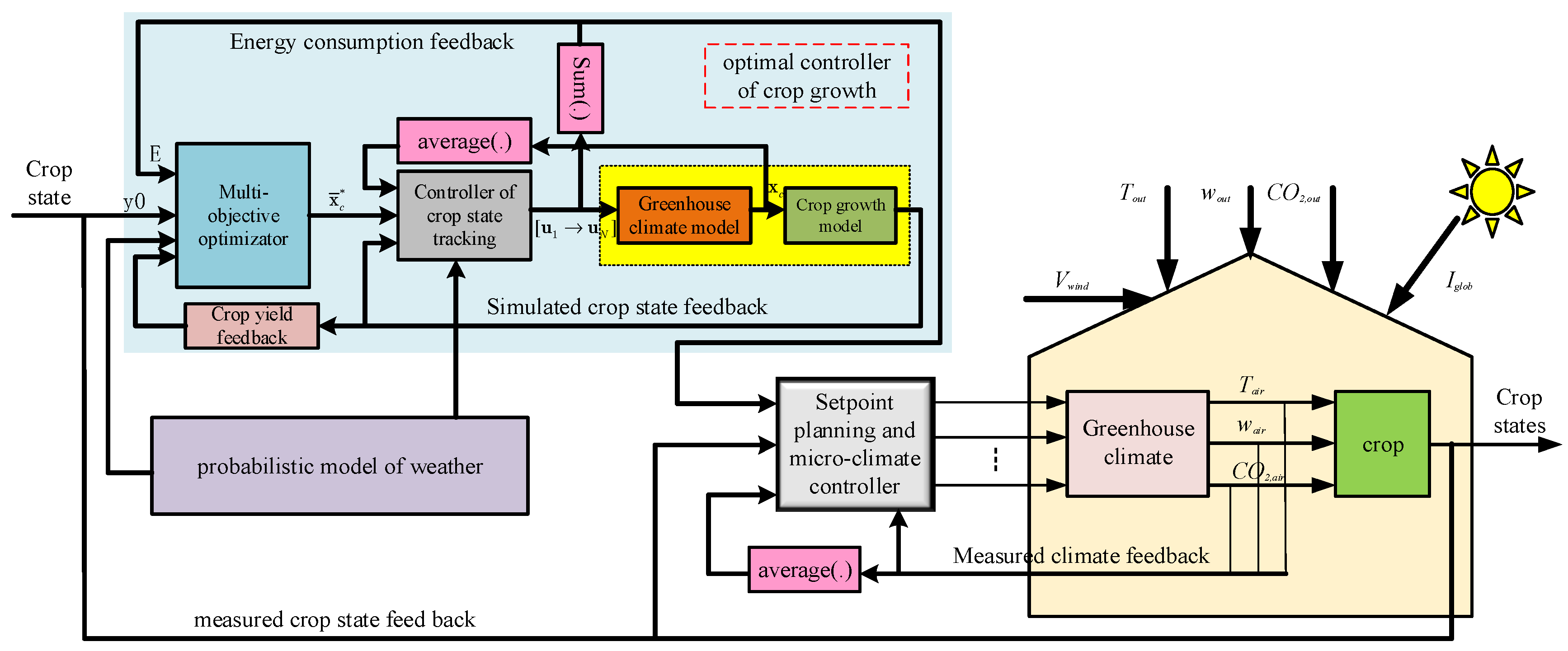
where $x_a$, $x_c$ are the indoor climate states and crop growth states, respectively; $v$ and $u$ are the weather and control inputs of the actuators respectively; and $F_a(\cdot )$ and $F_c(\cdot )$ represent the environment subsystem and crop growth subsystem, respectively. The entire greenhouse crop production control system can be considered as a typical dual closed-loop control system, as shown in Figure 1. The control system has two controllers, the outer loop controller is used to generate the daily setpoint of the greenhouse climate, and the inner loop controller is used to generate the control inputs of heating, fogging, ventilating, CO₂ enrichment and supplemental light to ensure the setpoint tracking control performance of the greenhouse climate.

Assuming that the crop-growth states and greenhouse climate can be accurately detected online, then the aim of greenhouse climate optimal control is to maximize the crop yield with the minimum energy input. However, due to both the great uncertainty of weather and to model error, the controllers must have the ability to correct the control error according to real-time feedback, which means a good control approach is important. In fact, in the dual closed-loop control system, the outer loop controller is a setpoint optimiser, and the daily setpoint can be obtained by maximizing crop yield and minimizing energy consumption.

From the dynamic characteristics of both subsystems, it can be known that the response speed of the crop growth subsystem is much slower than that of the greenhouse environment subsystem; thereby, the greenhouse crop production system behaves as a typical singular perturbation system with two time-scales [29,30,31,32]. In general, the greenhouse environment can be measured in real-time; for example, the microclimate can be detected every 5 min, but the sampling period of the crop growth states is set as 24 h. Therefore, the greenhouse climate setpoint generated by the outer controller is a daily average setpoint. Thus, a mechanism must be introduced to transform the daily average setpoint into the setpoint trajectory.

For some crops, such as tomato and cucumber, the crop yield can only be measured at harvest time, meaning that the overall crop growth and control process greenhouse climate must be simulated to estimate the crop yield and energy consumption. Then, by using the obtained control inputs and simulation climate, the energy consumption and crop yield can be calculated as follows:

$$E={\displaystyle {\int }_{t_0}^{t_f}{\displaystyle \sum _{i=1}^m{\alpha }_i{u}_i(t)dt}}$$

(3)

$$Y={\displaystyle {\int }_{t_0}^{t_f}{F}_c(x_a,x_c,w)dt}$$

(4)

where $t_0$, $t_f$ are the transplant time and harvest time, respectively; ${\alpha }_i$ is the capacity of the actuator; and $m$ denotes the number of actuators. If the greenhouse climate model and crop growth model have good simulation performance, then Equations (3) and (4) can accurately predict the total energy consumption and crop yield. Furthermore, the following important issues must be considered:

(1)

Transforming the daily average setpoints of greenhouse climate into the setpoint trajectory.

(2)

Studying an effective control strategy to ensure the desired control performance.

(3)

Developing a surrogate-based optimisation method to optimise the setpoint of greenhouse climate.

The full methodological diagram is shown in Figure 2.

2.3. Greenhouse Climate Model

As crop growth depends on the indoor microclimate, accurately simulating the greenhouse microclimate is important for the prediction of crop yield and energy consumption. Generally, the greenhouse climate is affected by greenhouse structure, materials, crop growth, weather and control operations. Due to the complexity of the heat transfer and mass exchange between inside and outside the greenhouse, it is difficult to accurately model the greenhouse climate. Therefore, considerable efforts have been made to study greenhouse climate modelling [17,33]. However, although some models have good simulation performance, their computations are expensive and are difficult to use for the global optimisation of the setpoints. To reduce the simulation time of greenhouse climate without loss of simulation performance, this work constructed a simple model with eight state variables based on the models developed by Van Ooteghem [34], Vanthoor [35], DE Zwart [36]. the model is described as follows:

$$\left\{\begin{array}{l}ca{p}_{air}{\dot{T}}_{Air}=Q_{Canair}+Q_{Pipeair}+Q_{Blowair}+I_{Sunair}-Q_{airFlr}-Q_{airout}-Q_{airTop}-Q_{airout\_Pad}-Q_{airFog}-Q_{airCov}\\ ca{p}_{Flr}{\dot{T}}_{Flr}=Q_{airFlr}+I_{SunFlr}-Q_{FlrSoil}-R_{FlrSky}\\ ca{p}_{Top}{\dot{T}}_{Top}=I_{SunTop}+Q_{airTop}-Q_{TopCov}-Q_{Topout}\\ ca{p}_{Co\nu }{\dot{T}}_{Co\nu }=I_{SunCov}+Q_{TopCov}+Q_{AirCov}-Q_{Covout}-R_{CovSky}\\ ca{p}_{w_{air}}{\dot{w}}_{Air}=M{C}_{Canair}+M{C}_{Padair}+M{C}_{Fogair}-M{C}_{airTop}-M{C}_{airout}-M{C}_{airCov}\\ ca{p}_{w_{Top}}{\dot{w}}_{Top}=M_{airTop}-M_{TopCov}-M_{Topout}\\ ca{p}_{C{O}_{2.air}}{\stackrel{.}{CO}}_{2,air}=C_{Extair}+C_{Padair}-C_{airCan}-C_{airTop}-C_{airout}\\ ca{p}_{C{O}_{2Top}}\dot{C}{O}_{2,Top}=C_{airTop}-C_{Topout}\end{array}\right.$$

(5)

where $T_{Flr}$ and $T_{Co\nu }$ are the temperature of floor and cover, respectively, and $T_{Air}$, $T_{Top}$ are the air temperature below and above thermal screen, respectively. $w_{Air}$, $w_{Top}$ are the humidity below and above the thermal screen, respectively, and ${\stackrel{.}{CO}}_{2,air}$, $C{O}_{2,Top}$ are the CO₂ concentrations. The nomenclature of the supplementary materials can be referred to for the other variables in Equation (5). The greenhouse interior is separated into upper and lower layers by thermal screens, so temperature, humidity, and CO₂ concentration in each layer are treated as separate environmental variables. There are 10 control variables in the model.

2.4. Setpoint Trajectory Programming

(1)

Temperature setpoint programming

According to crop growth models such as TOMGRO [37] and TOMSIM [25], crop growth is mainly affected by the average daily temperature, and the fluctuation of transient temperature does not have a large impact on crop growth when the ambient temperature fluctuates within the safe growth temperature range, such as 10~40 °C for a specific tomato cultivar. Therefore, the regulation of the temperature should focus on the daily average temperature rather than the transient temperature. Generally, the higher temperature contributes to photosynthesis, while the lower temperature can save much heating energy. Therefore, when programming the setpoint, we must maximize the photosynthesis rate and minimize the difference between indoor and outdoor temperatures as much as possible.

To achieve a good energy-saving performance in the greenhouse climate regulation process, the setpoint optimisation of indoor temperature must consider the following situations:

(1)

If the daily mean temperature setpoint is not higher than the daily average outdoor temperature, then the real-time setpoint of indoor temperature $T_{air}^{set}$ should not be higher than the outside temperature $T_{out}$. In this case, the heater must be turned off, and ventilation windows should be opened to regulate the indoor temperature. When the indoor temperature is higher than the setpoint due to solar radiation, the pad-and-fan system must be turned on to cool the greenhouse. The control strategies of ventilation and cooling are generated by the controller. As the energy consumption of the roof ventilation can be almost neglected, the main energy consumption mainly comes from the pad-and-fan system.

(2)

If the daily mean temperature is higher than the daily average outdoor temperature, and the average outdoor temperature during the night is higher than a given minimum temperature, then the temperature setpoint should be as close as possible to the outdoor temperature. In this case, the temperature inside the greenhouse can only be regulated by ventilation to avoid the activation of the heating system and the pad cooling system. During the day, the temperature setpoint may be set as a higher value due to the thermal effect of solar radiation. In this case, the higher temperature can enhance photosynthesis without consuming extra heating energy.

(3)

If the daily average outdoor temperature is lower than the temperature setpoint, and the outside temperature is smaller than the lower bound $T_{air}^{\min }$, then the temperature setpoint during the night should not be less than the lower bound.

In any case, the indoor temperature should not be higher than the upper bound $T_{air}^{\max }$ that the crop can tolerate. ${\overline{T}}_{air}^{set}$ denotes the daily mean temperature of a day, which represents the daily accumulated temperature; ${\overline{T}}_{out}$ denotes the average daily outdoor temperature; and ${\overline{T}}_{out}^{night}$ denotes the average temperature during the night outside the greenhouse.

Then, according to the three cases above, we can form the following rules for the planning of the temperature setpoint:

Rule 1:

if ${\overline{T}}_{air}^{set}\le {\overline{T}}_{out}$, then when $T_{out}<T_{air}^{\max }$, it can set $T_{air}^{set}=T_{out}$, otherwise it has $T_{air}^{set}=T_{air}^{\max }$.

Rule 2:

if ${\overline{T}}_{air}^{set}>{\overline{T}}_{out}$, and ${\overline{T}}_{out}^{night}>T_{air}^{\min }$, then the temperature setpoint can be programmed separately in different time period of a day, and there are two cases, as follows:

(a)

During the night: $T_{air}^{set}=T_{out}$

(b)

During the day: assume that there is an optimal temperature $T_{air}^{opt}$ for photosynthesis, then, when programming the temperature setpoint of the day, for a given accumulated temperature, the temperature setpoint should be as close as possible to the optimal temperature, but if the outdoor temperature is lower than the optimal temperature, the optimal photosynthetic temperature compensation must be carried out when the outdoor temperature is high, as shown in Figure 3. Thus, we can reduce the energy consumption of the heating. Generally, during such period, solar radiation is strong, and raising the temperature can improve photosynthesis. Therefore, it is reasonable to raise the temperature setpoint to the optimal photosynthetic temperature. If the outdoor temperature is higher than the upper bound $T_{air}^{\max }$, the setpoint must be set as $T_{air}^{set}=T_{air}^{\max }$.

Rule 3:

If ${\overline{T}}_{air}^{set}>{\overline{T}}_{out}$, and ${\overline{T}}_{out}^{night}\le T_{air}^{\min }$, i.e., the weather is cold, then the temperature setpoint should not be less than the lower bound $T_{air}^{\min }$ for the protection of the crop. However, from an energy-saving point of view, setting a lower temperature setpoint during the night can greatly reduce the energy of the heating when the temperature setpoint is not more than the upper bound $T_{air}^{\max }$. However, according to the photosynthesis model [38], if the light intensity is not sufficient, raising the temperature alone cannot significantly improve the photosynthesis rate, as shown in Figure 4. Consequently, during the periods 6:00~7:30 and 16:30~18:00, in which the light intensity is weak, the temperature setpoint should be set as a small value. The temperature setpoint can change with linear law during both periods, i.e., we can construct a daily trapezium setpoint trajectory, as shown in Figure 5.

During the period $t_{7:30}\to t_{16:30}$, the difference of the maximal and minimal temperature setpoints can be calculated as follows:

$$h=[{\overline{T}}_{air}^{day}-T_{air}^{set}(night)]{\displaystyle \frac{(t_{24:00}-t_{00:00})}{2(t_{7:30}-t_{6:00})}}$$

(6)

where ${\overline{T}}_{air}^{day}$ is the average temperature during the day; $T_{air}^{set}(night)$ is the temperature setpoint during the night; $t_{6:00}$ and $t_{7:30}$ represent the times 6:00 and 7:30, respectively; and $t_{00:00}$ and $t_{24:00}$ are the initial time and terminal time of a day, respectively. Then, the temperature setpoint during $t_{7:30}\to t_{16:30}$ can be determined as follows:

$$T_{air}^{set}(t_{7:30}\to t_{16:30})=T_{air}^{set}(night)+h$$

(7)

Because the setpoint during the day depends on ${\overline{T}}_{air}^{set}$ and $T_{air}^{set}(night)$, the setpoint during the night should be suitable, such that the setpoint during $t_{7:30}\to t_{16:30}$ may be close to $T_{air}^{opt}$ with the minimum energy consumption.

(2)

CO₂ concentration setpoint programming

The CO₂ concentration can significantly impact crop growth. Generally, under favourable light conditions, high CO₂ concentrations can greatly promote crop growth. However, if the light is not sufficient, then only increasing indoor CO₂ concentration cannot significantly improve photosynthesis [39,40]. Therefore, it is not reasonable to set a fixed CO₂ concentration. The indoor CO₂ concentration must be adjusted according to the light conditions. During the day, CO₂ concentration setpoint should change with the solar radiation, and higher solar radiation requires a higher CO₂ concentration setpoint. 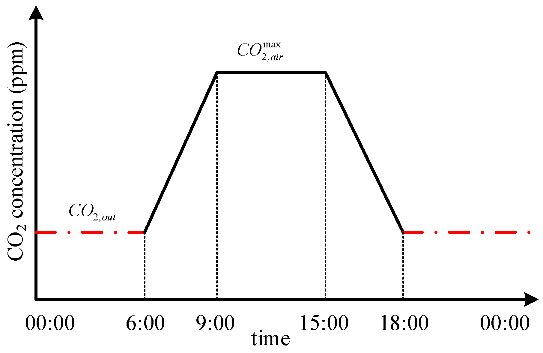If not considering the supplemental light at night, the CO₂ enrichment is not required to maintain the CO₂ concentration. As a result, we do not consider the nighttime setpoint trajectory programming. For a given maximum CO₂ concentration, the trajectory of the CO₂ concentration setpoint of a day can be constructed as a trapezoidal shape, as shown in Figure 6.

For the Shanghai region in winter, generally, the solar radiation gradually increases from 6:00, but before 9:00 is not strong. In this case, it is not suitable to set a higher CO₂ concentration. A reasonable method is to make the indoor CO₂ concentrations gradually increase with solar radiation. Similarly, the indoor CO₂ concentrations should be reduced between 15:00 and 18:00 due to the sunset. However, the setting should not be lower than the outdoor CO₂ concentration, and the lower bound of the indoor CO₂ concentration setpoint can be equal to the outdoor CO₂ concentration.

2.5. Model-Based Interpolation Control Strategy

If the optimal setpoint of the greenhouse climate is obtained, then an effective control strategy must be introduced to ensure the tracking performance of the optimal setpoint. Many control methods have been proposed over the years to solve the greenhouse climate control problem. However, as the greenhouse climate is a strongly coupled nonlinear system, some traditional control methods, such as PID control, often have difficulty solving the multi-factor coordination control problem of greenhouse climate, while, though many Lyapunov-based control algorithms can achieve a good control performance in the simulation, they are usually complex, and require a small control step size. As a result, those control methods are difficult to be applied in the control engineering practices. In most cases, the threshold switch control is still the main control method in practice. As the response of crop growth to the environment is usually robust, a small control error may not significantly impact crop growth. Therefore, it is not necessary to drive the greenhouse climate to completely track the setpoint, i.e., a small tracking control error is acceptable.

To prevent the actuator from operating too frequently, the control step size should be reasonably set, such as at 15 min, or even 1 h, but must meanwhile ensure stability and control performance. In general, the control inputs can be expressed as a function with respect to the indoor and outdoor environmental factors, i.e., it can be described as follows:

$$u=f(x,x^{set},v,)$$

(8)

where $f(\cdot )$ represents a control law.

If using a greenhouse climate model to simulate the control under various conditions, then we can obtain many control rules. Based on the control rule samples, a control rule library can be constructed. In the control process, a new control strategy can be derived from the control rule library according to a given control condition. The main idea is to first generate a number of samples of initial indoor climate and weather, as well as a set of setpoint samples. For each setpoint sample, different initial conditions result in different control strategies. Suppose that there are L samples of initial states and weather, and S setpoint samples, then, for a given initial condition and setpoint, a one-step forward control simulation is carried out to search for a control strategy in the decision space to ensure the tracking error below a given threshold, as shown in Figure 7. The details of this implementation procedure are presented in the supplementary materials. For each setpoint, N initial conditions can result in N control rules, thereby, for S samples of the setpoint, $S\times L$ control rules can be obtained. We can use the control rules in a control rule library. If the number of the initial condition samples is large enough, the control rule library can cover most control strategies of the control process. Therefore, it can easily generate a real-time control strategy using the interpolation method.

On hot days, this often uses ventilation or a wet curtain to cool the greenhouse, while if the weather is cold, the heating operation must be performed to maintain the indoor temperature. Due to the different heat dissipation conditions of greenhouses during the day and at night, such as the influence of solar radiation during the day, different interpolation surfaces of control rules for both daytime and nighttime must be constructed. As this study focuses on the cultivation period from 1 September to 31 December, the weather changes from hot to cold. In the early stages of the cultivation period, the wet curtain was usually turned on to cool the greenhouse, while, in later stages, heating is required to raise the indoor temperature. During this period, several control operations, including wet curtain cooling, roof ventilation, thermal screen, shading and heating are considered in the overall control process of the greenhouse climate.

As the indoor temperature is the primary environmental factor that greatly influences the crop growth, the control performance of the indoor temperature must firstly be ensured. Under such prerequisites, the light and CO₂ concentration can be regulated to further improve crop growth. When obtaining the control strategies of the ventilation and pad, the supply fluxes of the supplemental light and CO₂ can be calculated by the air fluxes. According to the energy dissipation conditions inside the greenhouse, four control strategy libraries can be built for different cases.

(1)

Outside temperature is lower than the indoor temperature setpoint, i.e., $T_{out}<T_{air}^{set}$

Such a case implies that, if we want to drive the indoor temperature to the setpoint, the heating system must be turned on to provide enough heat. However, during the day, if the difference between the outdoor temperature and the temperature setpoint is small, then the solar radiation can compensate for heat loss to maintain the indoor temperature, i.e., the heating operation may not be adopted. Therefore, the control rule libraries of the nighttime and daytime must be established separately, i.e., the following sub-cases can be considered:

(1)

Night:

The heating control input is mainly affected by the indoor temperature setpoint and outdoor temperature, thereby, if ignoring the indoor temperature control error, the heating control inputs at night can be expressed as ${\widehat{u}}_{hot}=f_{hot}(T_{air}^{set},T_{out})$. The interpolation surfaces of both control operations can be obtained by simulating a one-step forward control under different indoor temperature setpoints and outdoor temperature conditions, and the construction process of the interpolation surfaces is demonstrated by Algorithm S1 in the Supplementary Materials.

In this study, the maximal control error of the temperature is set as 0.5 °C, and, at night, the domain of the temperature setpoint is defined as $T_{air}^{set}\in [12,30]$ and the outside temperature changes within $T_{out}\in [0,30]$. The initial values of the floor temperature, top temperature and cover temperature are set as $T_{Alr}=T_{air}-2$, $T_{Top}=T_{air}-0.5$, $T_{Cov}=T_{out}+0.5$, respectively, meaning that we can then obtain the interpolation surfaces of the heating operation for two cases during the night, as shown in Figure 8.

As depicted in Figure 8, it is evident that the higher the temperature setpoint and the lower the outdoor temperature, the greater power of the heating is required to maintain the temperature setpoint. Consequently, this leads to an increase of energy consumption. However, under cold weather conditions, unfolding the thermal screen at night can reduce the energy consumption of the heating by approximately 10%. Moreover, when the temperature setpoint is close to the outdoor temperature, the energy consumption does not increase, as shown in Figure 8, because the heat transferred from the ground to the indoor air can compensate for the heat loss caused by the low outdoor temperature.

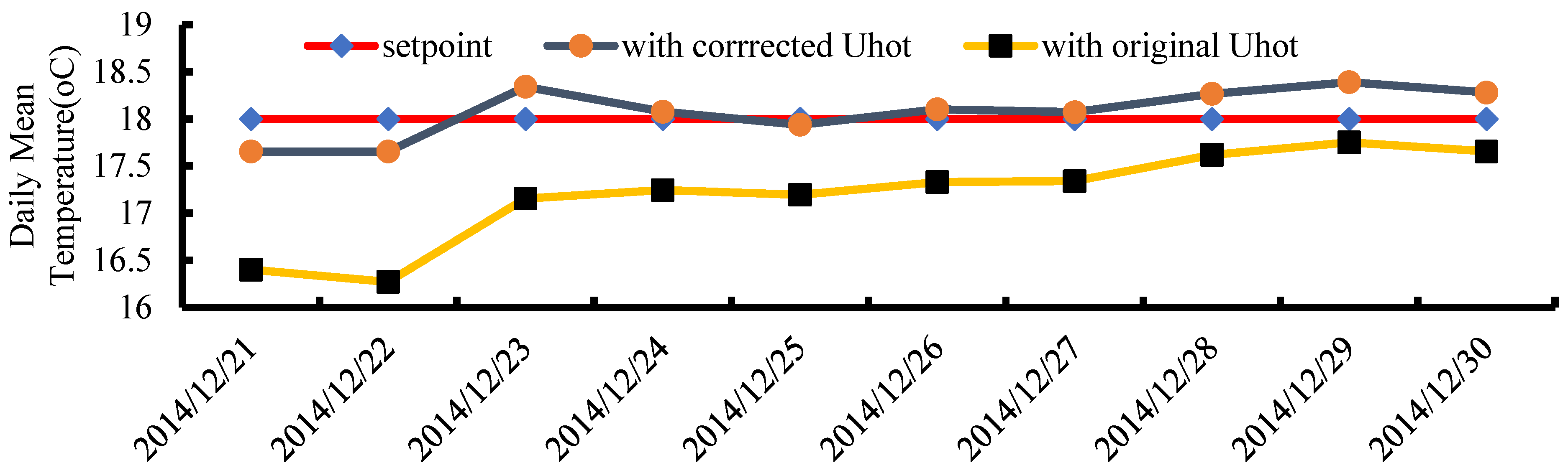
Under the given initial condition of greenhouse climate, the heating control strategy derived from the interpolation surface can ensure a control error not exceeding 0.5 °C. However, since the initial conditions of the actual control process may be different from the conditions of the one-step forward control simulation, the control strategy derived from the interpolation surface may lead to a larger control error than 0.5 °C. Therefore, the control strategy derived from the interpolation surface must be corrected according to the actual initial condition and control error, i.e., the corrected control strategy can be expressed as follows:

$$u_{hot}^{night}=f(T_{air}^{set},T_{out})+{\alpha }_{Flr}^{night}(T_{air}-T_{Flr}-2)+{\alpha }_{Top}^{night}(T_{air}-T_{Top}-0.5)-{\alpha }_{Cov}^{night}(T_{out}-T_{Cov}+0.5)+{\alpha }_e^{night}(T_{air}^{set}-T_{air})$$

(9)

where ${\alpha }_{Flr}^{night}$, ${\alpha }_{Top}^{night}$, ${\alpha }_{Cov}^{night}$ are the correction parameters of the floor temperature, the temperature of the top temperature and cover temperature, respectively, and ${\alpha }_e^{night}$ is the correction parameter of control error.

(2)

Daytime:

Besides the outdoor temperature and indoor temperature setpoint, the control input of heating during the day is also influenced by solar radiation. Strong solar radiation can reduce heat loss, meaning that the heating operation may not be turned on for energy saving. In some cases, roof windows may be opened to cool the greenhouse. However, if solar radiation cannot compensate for the heat loss, then the heating system must be activated to maintain the temperature. Therefore, both heating and ventilation operations during the day can be described as follows:

$${\widehat{u}}_{hot}=f(T_{air}^{set},T_{out},I_{glob})$$

(10)

$${\widehat{u}}_{roof}=f(T_{air}^{set},T_{out},I_{glob})$$

(11)

Generally, one can assume that the outdoor temperature, the temperature setpoint and the solar radiation are bounded by $T_{out}\in [T_{out}^{\min },T_{out}^{\max }]$, $T_{air}^{set}\in [T_{air}^{set,\min },T_{air}^{set,\max }]$,$I_{glob}\in [I_{glob}^{\min },I_{glob}^{\max }]$, respectively. In this study, the domains of these three parameters are respectively set to $T_{out}\in [0,30]$, $T_{air}^{set}\in [15,30]$, and $I_{glob}\in [0,900]$. The construction process of the daytime control rule libraries is similar. Due to the difference of the control conditions, the actual heating and ventilation control strategies must be corrected:

$$u_{hot}^{day}=f(T_{air}^{set},T_{out},I_{glob})+{\alpha }_{Flr}^{day}(T_{air}-T_{Flr}-2)+{\alpha }_{Top}^{day}(T_{air}-T_{Top}-0.5)-{\alpha }_{Cov}^{day}(T_{out}-T_{Cov}+0.5)+{\alpha }_e^{day}(T_{air}^{set}-T_{air})$$

(12)

$$u_{roof}=f(T_{air}^{set},T_{out},I_{glob})-{\gamma }_{roof}^{day}(T_{air}^{set}-T_{air})$$

(13)

where ${\alpha }_{Flr}^{day}$, ${\alpha }_{Top}^{day}$, ${\alpha }_{Cov}^{day}$, ${\alpha }_e^{day}$, ${\gamma }_{roof}^{day}$ are the correction parameters.

(1)

Outside temperature is higher than the temperature, i.e., $T_{out}\ge T_{air}^{set}$

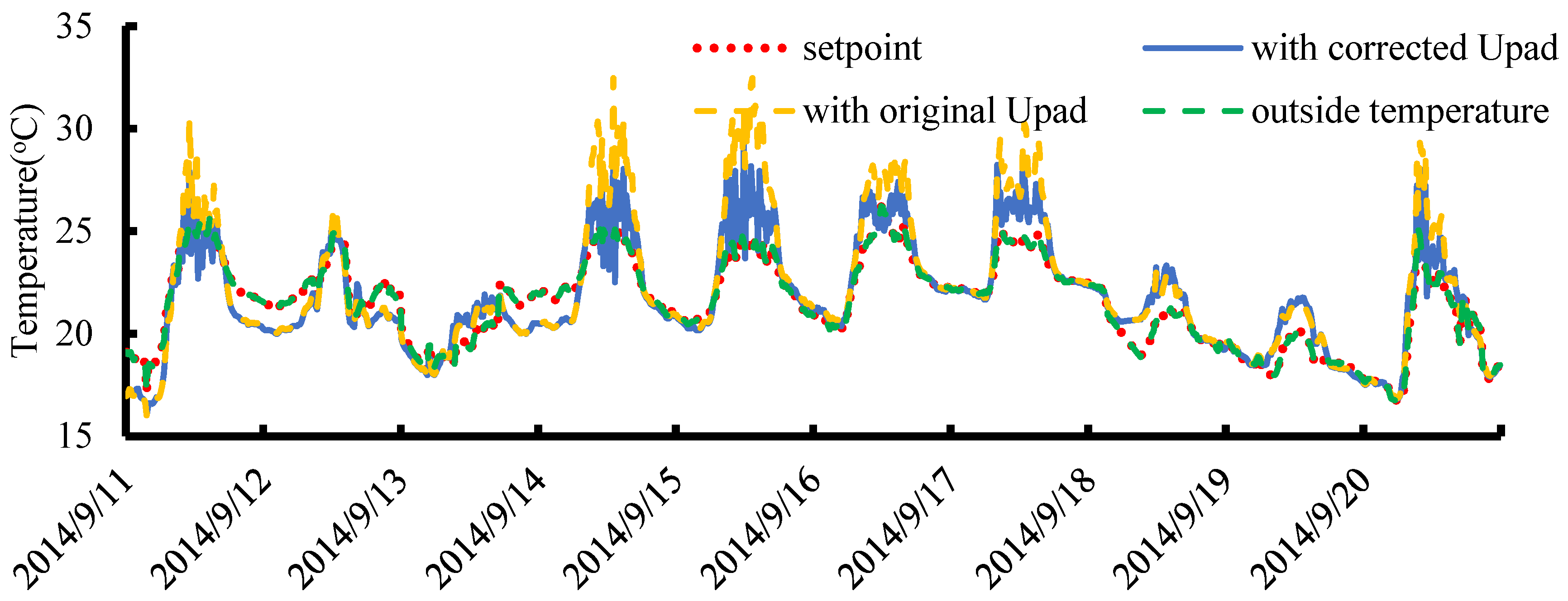
This case requires the activation of ventilation and pad cooling systems to decrease the temperature. If the pad cooling system has sufficient capacity, the indoor temperature can be adjusted to any reasonable setpoint. However, during nighttime and daytime, the factors that influence the control strategy of the pad are different. The control of the pad at night is primarily influenced by outdoor temperature and indoor temperature set value, whereas during the day it is affected by outdoor temperature, indoor temperature setpoint, and solar radiation. Therefore, the control input of the pad during nighttime and daytime can be respectively expressed as follows:

$${\widehat{u}}_{pad}^{night}=f(T_{air}^{set},T_{out})$$

(14)

$${\widehat{u}}_{pad}^{day}=f(T_{air}^{set},T_{out},I_{glob})$$

(15)

In the control process, one can use the measured greenhouse climate and the control error to correct the control inputs:

$${\widehat{u}}_{Pad}^{night}=f(T_{air}^{set},T_{out})+{\beta }_{Flr}^{night}(T_{air}-T_{Flr}-2)+{\beta }_{Top}^{night}(T_{out}-T_{Top}+1)+{\beta }_{Cov}^{night}(T_{out}-T_{Cov}+0.5)+{\beta }_e^{night}(T_{air}^{set}-T_{air})$$

(16)

$${\widehat{u}}_{pad}^{day}=f(T_{air}^{set},T_{out},I_{glob})+{\beta }_{flr}^{day}(T_{air}-T_{flr}-2)+{\beta }_{top}^{day}(T_{out}-T_{top}+1)+{\beta }_{\mathrm{cov}}^{day}(T_{out}-T_{\mathrm{cov}}+0.5)+{\beta }_e^{day}(T_{air}^{set}-T_{air})$$

(17)

where ${\beta }_{Flr}^{night}$, ${\beta }_{Top}^{night}$, ${\beta }_{Cov}^{night}$, ${\beta }_e^{night}$, ${\beta }_{Flr}^{day}$, ${\beta }_{Top}^{day}$, ${\beta }_{Cov}^{day}$, ${\beta }_e^{day}$ are the correction parameters.

The setting up process of the control rule libraries of the pad cooling and roof ventilation at night is demonstrated by Algorithm S2 in the Supplementary Material, and the setting up process of the control rule library during the day is similar.

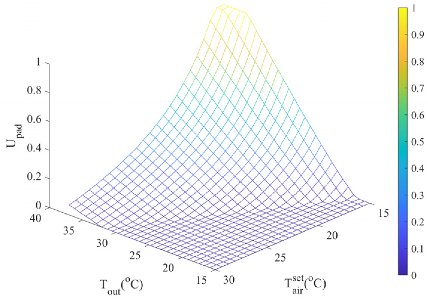
When the outdoor temperature is not less than the indoor temperature setpoint, we can obtain the interpolation surface of the pad control rule at night, as shown in Figure 9.

Although the corrected control strategy can achieve better control performance, it significantly depends on the correction coefficients. Therefore, the correction coefficients must be optimized to ensure the control performance. There are 17 parameters, and the parameter optimisation can be performed by two steps:

Step 1: By selecting a certain cold period of a year, such as 10–20 December 2014 in the Shanghai area, then the heating and ventilation control inputs can be corrected by minimizing the root mean square error:

$$\begin{array}{l}{\theta }_{hot}^{*}=\arg \underset{{\theta }_{hot}\in \Omega }{\min }\sqrt{{\displaystyle \frac{1}{n}}{\displaystyle \sum _{i=1}^n{\left(T_{air}^{set}(i)-T_{air}(i)\right)}^2}}\\ s.t.{\dot{x}}_a=F(x_a,x_c,v,u({\theta }_{hot}))\\ {\theta }_{hot}=[{\alpha }_{Flr}^{day},{\alpha }_{Top}^{day},{\alpha }_{Cov}^{day},{\alpha }_{Flr}^{night},{\alpha }_{Top}^{night},{\alpha }_{Cov}^{night},{\alpha }_e^{day},{\alpha }_e^{night},{\gamma }_{roof}^{day}]\end{array}$$

(18)

where $n$ is the number of the samples.

Step 2: By selecting a certain warm period of a year, the pad control input can be corrected by solving the following optimisation problems:

$$\begin{array}{l}{\theta }_{pad}^{*}=\arg \underset{{\theta }_{pad}\in \Omega }{\min }\sqrt{{\displaystyle \frac{1}{n}}{\displaystyle \sum _{i=1}^n{\left(T_{air}^{set}(i)-T_{air}(i)\right)}^2}}\\ s.t.{\dot{x}}_a=F(x_a,x_c,v,u({\theta }_{pad}))\\ {\theta }_{Pad}=[{\beta }_{Flr}^{day},{\beta }_{Top}^{day},{\beta }_{Cov}^{day},{\beta }_e^{day},{\beta }_{Flr}^{night},{\beta }_{Top}^{night},{\beta }_{Cov}^{night},{\beta }_e^{night}]\end{array}$$

(19)

In this study, the particle swarm optimisation method was used to solve both optimisation problems, so that the best correction coefficient could then be obtained, as shown in

Table 1. Correction factors for greenhouse heating, pad and fans and ventilation control operations based on the control rule library.

Parameter	Value	Parameter	Value
${\alpha }_{Flr}^{day}$	4.1418	${\beta }_{Flr}^{day}$	−1.196 × 10−3
${\alpha }_{Top}^{day}$	1.6047	${\beta }_{Top}^{day}$	4.916 × 10−2
${\alpha }_{Cov}^{day}$	2.2473	${\beta }_{Cov}^{day}$	4.591 × 10−2
${\alpha }_{Flr}^{night}$	1.0628	${\beta }_e^{day}$	−7.163 × 10−2
${\alpha }_{Top}^{night}$	0.5463	${\beta }_{Flr}^{night}$	8.963 × 10−2
${\alpha }_{Cov}^{night}$	1.7574	${\beta }_{Top}^{night}$	−1.084 × 10−2
${\alpha }_e^{day}$	7.2620	${\beta }_{Cov}^{night}$	1.971 × 10−3
${\alpha }_e^{night}$	9.2030	${\beta }_e^{night}$	9.402 × 10−2
${\gamma }_{roof}^{day}$	0.07614

.

Indoor CO₂ concentration is an important factor that can affect crop growth, and high-tech agricultural greenhouses are usually equipped with CO₂ enrichment systems. CO₂ enrichment is usually carried out during the day, and, generally, the more active the photosynthesis is, the more CO₂ is consumed. Therefore, the CO₂ enrichment system is required to provide a significant amount of CO₂. Additionally, the ventilation and pad cooling can also affect indoor CO₂ concentration. As the appropriate temperature is the basic condition for crop growth, the control index of the indoor temperature must be ensured as a priority. Some regulation operations, such as ventilation and pad cooling, are always used to ensure the control performance of the temperature. Under such a premise, if the CO₂ concentration dynamics can be ignored, then the control input of the CO₂ enrichment can be derived based on the steady-state equation, which can be expressed as follows:

$$U_{C{O}_2}=(C_{Padair}+C_{airCan}+C_{airTop}+C_{Aarout})/{\Phi }_{C{O}_2}$$

(20)

where ${\Phi }_{C{O}_2}$ is the capacity of the CO₂ enrichment system (mg/(s·m²)) and was set to 6 mg·s⁻¹·m⁻² in this study. Considering that the CO₂ concentration may not always be maintained at its setpoint and that different initial CO₂ concentrations may require different CO₂ supplies, then, to reduce the control error of the CO₂ concentration, a control error correction term and a compensation term for the ventilation control can be introduced to the steady-state control law of Equation (24). The steady-state control law can then be rewritten as follows:

$$U_{C{O}_2}=\left[{\gamma }_{1,C{O}_2}{C}_{Padair}+{\gamma }_{2,C{O}_2}{C}_{airCan}+{\gamma }_{3,C{O}_2}{C}_{airTop}+{\gamma }_{4,C{O}_2}{C}_{airout}+{\alpha }_{C{O}_2}(C{O}_{2,air}^{set}-C{O}_{2,air})+{\alpha }_{roof}{U}_{roof}\right]/{\Phi }_{C{O}_2}$$

(21)

where $U_{C{O}_2}\in [0,1]$, and the correction parameters ${\gamma }_{1,C{O}_2}$, ${\gamma }_{2,C{O}_2}$, ${\gamma }_{3,C{O}_2}$, ${\gamma }_{4,C{O}_2}$ reflect the effect of the ventilation and photosynthesis on the indoor CO₂ concentration, and ${\alpha }_{C{O}_2}$ is the correction parameter of the control error. To maintain the desired temperature, the heating and ventilation may be active at the same time, which implies that the ventilation results in additional CO₂ loss. Therefore, a ventilation correction term is introduced to the CO₂ control law to compensate for the CO₂ loss, and ${\alpha }_{roof}$ is the correction parameter.

The correction factors can be obtained by solving the following minimization problem:

$$\begin{array}{l}{\gamma }_{C{O}_2}^{*}=\arg \underset{{\theta }_{C{O}_2}\in \Omega }{\min }\sqrt{{\displaystyle \frac{1}{n}}{\displaystyle \sum _{i=1}^n{\left(C{O}_{2,air}^{set}(i)-C{O}_{2,air}(i)\right)}^2}}\\ s.t.{\dot{x}}_a=F(x_a,x_c,w,u({\gamma }_{C{O}_2}))\\ {\gamma }_{C{O}_2}=[{\gamma }_{1,C{O}_2},{\gamma }_{2,C{O}_2},{\gamma }_{3,C{O}_2},{\gamma }_{4,C{O}_2},{\alpha }_{C{O}_2},{\alpha }_{roof}]\end{array}$$

(22)

Under warm weather conditions, the ventilation should be used to cool the greenhouse as a priority, and we should avoid using the pad to cool the greenhouse as much as possible for energy saving. In this case, the indoor CO₂ concentration is usually close to the outdoor CO₂ concentration. Even if the CO₂ enrichment system is turned on, it is difficult to raise the indoor CO₂ concentration due to the ventilation. Consequently, the CO₂ enrichment system is generally not activated in warm weather conditions. To determine correction coefficients of the CO₂ control law, this study utilized outdoor climate data measured from 10 to 20 December 2014 to train the control process, the obtained optimal correction coefficients are presented in

Table 2. Correction parameters of CO₂ input law.

Parameter	${\mathit{\gamma }}_{1,\mathit{C}{\mathit{O}}_2}$	${\mathit{\gamma }}_{2,\mathit{C}{\mathit{O}}_2}$	${\mathit{\gamma }}_{3,\mathit{C}{\mathit{O}}_2}$	${\mathit{\gamma }}_{4,\mathit{C}{\mathit{O}}_2}$	${\mathit{\alpha }}_{\mathit{C}{\mathit{O}}_2}$	${\mathit{\alpha }}_{\mathit{r}\mathit{o}\mathit{o}\mathit{f}}$
value	7.5266	0.9173	0.6626	1.5142	0.0010	1.0000

.

Considering that the outdoor temperature is not less than the indoor temperature setpoint under warm weather conditions, the ventilation can be used to adjust the indoor temperature, such that the CO₂ enrichment may not be activated. The control strategy of the CO₂ enrichment can be generated according to Algorithm S3, which is presented in the Supplementary Material.

2.6. Global Optimisation of Setpoint

The setpoint of greenhouse climate has a significant impact on crop yields and energy consumption. In a broad sense, greenhouse climate setpoints can be understood in four ways. The first is the average of environmental variables of the entire crop growth period; the second is the average of environmental variables of a growth stage; the third is the daily average of the greenhouse climate; and the fourth is the real-time setpoints of each control step, which represent the desired trajectory of the indoor environment. If we want to achieve globally optimal results in terms of energy consumption and crop yield, the best way is to directly optimize the real-time setpoints. However, there are several challenges. Firstly, the setpoint of each control step must be considered a decision variable of the nonlinear optimisation problem; however, as the growth period usually spans several months, the number of decision variables is very large. In this case, the optimisation algorithms have great difficulty finding the optimal solutions. Secondly, the objective functions are very expensive, and a single optimisation process may take several dozen days, thereby it is difficult to ensure the real-time performance of the optimisation results.

In contrast to the global optimisation of the real-time setpoints, the optimisations of the former three setpoints are much simpler due to the smaller number of decision variables. As the average of the climate variables of the overall growth period can reflect the total energy consumption and the final crop yield, this study focuses on the optimisation of the global average of the greenhouse climate. As the setpoints on the different senses have different timescales, an allocation strategy must be introduced to transform the setpoint with large timescales into the setpoint with small timescales. For making a trade-off between reducing energy-saving and promoting photosynthesis, the principle of such an allocation strategy is that, if a day is cold, then a small average temperature setpoint should be set, while, when the solar radiation is strong, a high setpoint can be defined for the CO₂ concentration. According to such a principle, an allocation strategy for the accumulated temperature and the average CO₂ concentration is proposed in this study.

(1)

Allocation strategy for temperature setpoint

Assuming that the daily average of the outdoor temperature $\left[{\overline{T}}_{out,1},\cdots ,{\overline{T}}_{out,m}\right]$ of the overall growth period is known, where $m$ represents the number of days of the entire growth period and the average temperature is given as ${\overline{T}}_{overall}$, then the daily mean temperature can be determined by two cases:

Case1: if ${\overline{T}}_{out,i}\ge {\overline{T}}_{overall}$, then ${\overline{T}}_{air,i}={\overline{T}}_{out,i}$

Case2: ${\overline{T}}_{out,i}<{\overline{T}}_{overall}$

In case 2, denotes ${\left[{\overline{T}}_{out,1},\cdots ,{\overline{T}}_{out,K}\right]}_{cold}$ as the outdoor temperature, then the total cumulative temperature compensation can be calculated as follows:

$$S{T}_{overall}={\displaystyle \sum _{j=1}^K\left({\overline{T}}_{overall}-{\overline{T}}_{out,j}\right)}$$

(23)

where $K$ is the number of days in which the average daily outdoor temperature is below ${\overline{T}}_{overall}$.

In general, if the light is sufficient, then the photosynthesis is active when the climate is warm. For instance, when the ambient temperature is close to 25 °C, the tomato crop has optimal photosynthesis. To improve the crop growth, the indoor temperature should be adjusted to the optimal temperature $T_{air}^{opt}$. When the weather is cold, if the temperature setpoint at night is set as $T_{air}^{\min }$, then, according to Equations (10) and (11), the temperature setpoint during the day may be set to the optimal ambient temperature $T_{air}^{opt}$, and the corresponding average daily temperature is ${\overline{T}}_{air}^{opt}$.

The aim of accumulated temperature compensation is to compensate the average temperature of each day to the optimal average temperature according to the total accumulated temperature and the change in the outdoor temperature.

If the average outside temperature of a day is high, then the temperature setpoint of this day should be compensated to the optimal average temperature ${\overline{T}}_{air}^{opt}$ as a priority. Conversely, if a day is cold, then it should be allocated less accumulated temperature for reducing energy consumption. In any case, the temperature setpoint must be no less than the lower bound $T_{air}^{\min }$. Therefore, before performing the accumulation temperature compensation, we must determine a reference temperature, as follows:

$${\overline{T}}_{air,j}^{ref}=\left\{\begin{array}{cc}{\overline{T}}_{out,j}\hfill & {\overline{T}}_{out,j}\ge T_{air}^{\min }\\ T_{air}^{\min }\hfill & elsewise\end{array}\right.$$

(24)

The remaining accumulated temperature can be calculated as follows:

$${\stackrel{\wedge }{ST}}_{overall}=S{T}_{overall}-{\displaystyle \sum _{j=1}^K\left({\overline{T}}_{air,j}^{ref}-{\overline{T}}_{air,j}\right)}$$

(25)

From the perspective of reducing energy consumption and promoting crop growth, a day with the highest reference temperature has the priority to compensate the accumulation temperature, and the amount of the compensation temperature is defined as follows:

$$\Delta T={\overline{T}}_{air}^{opt}-\max \left\{{\overline{T}}_{air,j}^{ref}\right\}$$

(26)

If the amount of the accumulated temperature compensation $K\cdot \Delta T$ is greater than the total residual accumulated temperature ${\stackrel{\wedge }{ST}}_{overall}$, then $\Delta T$ must be reduced, and the updated law is as follows:

$$\Delta T=\Delta T-T_{\beta }$$

(27)

where $T_{\beta }$ is the correction parameter. When ${\stackrel{\wedge }{ST}}_{overall}=K\cdot \Delta T$, then the updating process is terminated and the reference temperature can be updated as follows:

$${\overline{T}}_{air,j}^{ref}={\overline{T}}_{air,j}^{ref}+\alpha \cdot \Delta T$$

(28)

If ${\overline{T}}_{air,j}^{ref}={\overline{T}}_{air}^{opt}$, then $\alpha$ can be set as 0, otherwise, it can be set as 1, i.e., if the reference temperature is close to the average optimal temperature, then the temperature compensation is not performed. Until ${\stackrel{\wedge }{ST}}_{overall}$ becomes zero, the whole accumulated temperature compensation and average temperature allocation process is terminated, as shown in Figure 10.

(2)

Allocation strategy for CO₂ concentration setpoint

When optimizing the CO₂ concentration setpoint, we must consider two boundary problems. Firstly, the setpoint cannot be lower than the outdoor CO₂ concentration. Secondly, we should not exceed the CO₂ saturation point of photosynthesis. Typically, if the indoor CO₂ concentration is lower than the outdoor CO₂ concentration, then we can use the ventilation operation to promote indoor CO₂ concentration at a low cost. Therefore, the indoor CO₂ concentration setpoint should not be lower than the outdoor CO₂ concentration. According to the photosynthesis theory, if the CO₂ concentration exceeds the saturation point, it cannot greatly enhance the photosynthetic rate, resulting in the wastage of CO₂ and the increase of the regulation costs.

Let $C{O}_{2,air}^{\min }$, $C{O}_{2,air}^{\max }$ be the maximum and minimum setpoint of the CO₂ concentration, respectively, and ${\overrightarrow{CO}}_{2,air}^{overall}$ is the average CO₂ concentration of the overall growth period. Then, referring to the lower bound of the CO₂ concentration setpoint, the total compensated amount of CO₂ can be calculated as follows:

$$S{C}_{overall}=M\cdot ({\overrightarrow{CO}}_{2,air}^{overall}-C{O}_{2,air}^{\min })$$

(29)

where $\left[{\overline{I}}_{glob,1},\cdots ,{\overline{I}}_{glob,M}\right]$ denotes the average daily solar radiation of the overall growth period. If the initial value of the CO₂ concentration setpoint is set as $C{O}_{2,air}^{\min }$, then the daily CO₂ concentration setpoint can be iteratively calculated, and the update equation can be described as follows:

$$C{O}_{2,air,i}^{set}=C{O}_{2,air,i}^{set}+{\beta }_i\cdot S{C}_{overall}$$

(30)

where

$${\beta }_i={\displaystyle \frac{I_{glob,i}}{sum\left(\left[I_{glob,1},\cdots ,I_{glob,M}\right]\right)}}$$

However, if the amount of the CO₂ mass is proportionally allocated with the solar radiation, this may lead the CO₂ concentration setpoint to exceed the preset maximum value $C{O}_{2,air}^{\max }$, meaning that the updated setpoint must be corrected, i.e., if ${\beta }_i\cdot S{C}_{overall}>(C{O}_{2,air}^{\max }-C{O}_{2,air}^{\min })$, then $C{O}_{2,air,i}^{set}=C{O}_{2,air}^{\max }$, and the solar radiation of the i-th day is removed from the set $\left[{\overline{I}}_{glob,1},\cdots ,{\overline{I}}_{glob,M}\right]$, i.e., $\left[{\overline{I}}_{glob,1},\cdots ,{\overline{I}}_{glob,M}\right]\backslash {\overline{I}}_{glob,i}$. Consequently, the CO₂ concentration setpoint that does not reach the maximum value will be re-allocated according to the residual compensation $\overrightarrow{SC}=sum(C{O}_{2,air}^{set}-C{O}_{2,air}^{\min })$, and the update equation can be described as follows:

$$C{O}_{2,air,i}^{set}=C{O}_{2,air,i}^{set}+{\widehat{\beta }}_i\cdot {\overrightarrow{SC}}_{overall}$$

(31)

where

$${\widehat{\beta }}_i={\displaystyle \frac{I_{glob,i}}{sum\left(\left[I_{glob,1},\cdots ,I_{glob,M}\right]\backslash I_{glob,j}\right)}}$$

The updating process will not stop until ${\overrightarrow{SC}}_{overall}=0$.

(3)

Total energy consumption and crop yield distribution for different setpoints

The optimisation of the greenhouse climate setpoint includes several steps. In this optimisation process, the overall average setpoint is gradually transformed into the daily average setpoint, and then into the real-time trajectory. The optimal setpoint can be obtained by maximizing the financial return, which can be expressed as follows:

$$\begin{array}{l}\underset{[{\overline{T}}_{overall},{\overrightarrow{CO}}_{2,air}^{overall}]\in \Omega }{\max }J=p_y\cdot Y-p_e\cdot E\\ s.t.{\dot{x}}_a=F_a(x_a,x_c,w,u)\\ {\dot{x}}_c=F_c(x_a,x_c,w)\end{array}$$

(32)

where $p_y$ and $p_e$ represent the prices of the agricultural product and energy, respectively. $E$ represents a generalized energy consumption which includes the energy of heating and the supply of the CO₂.

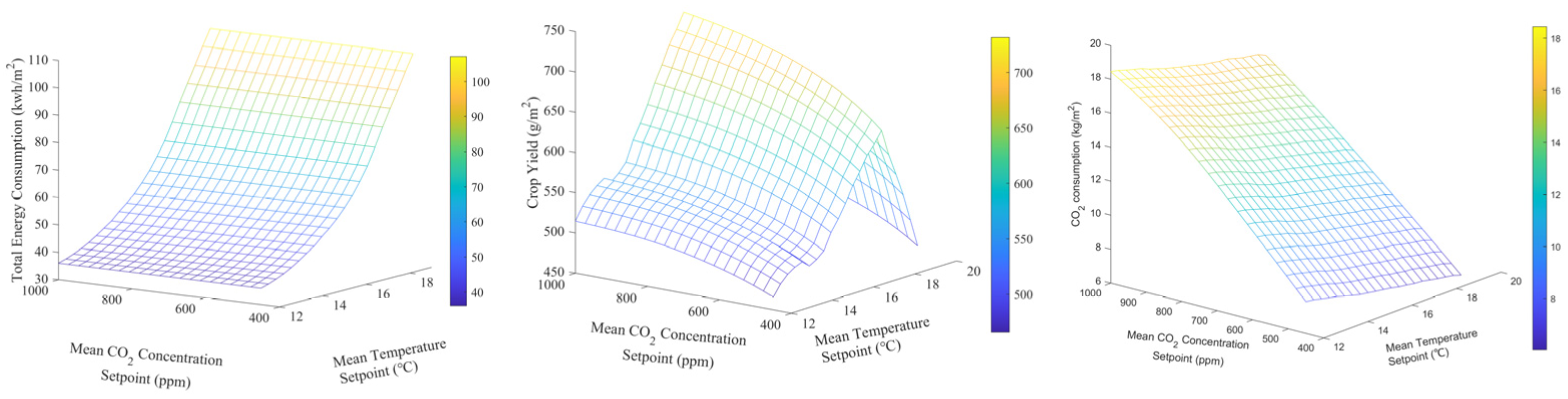
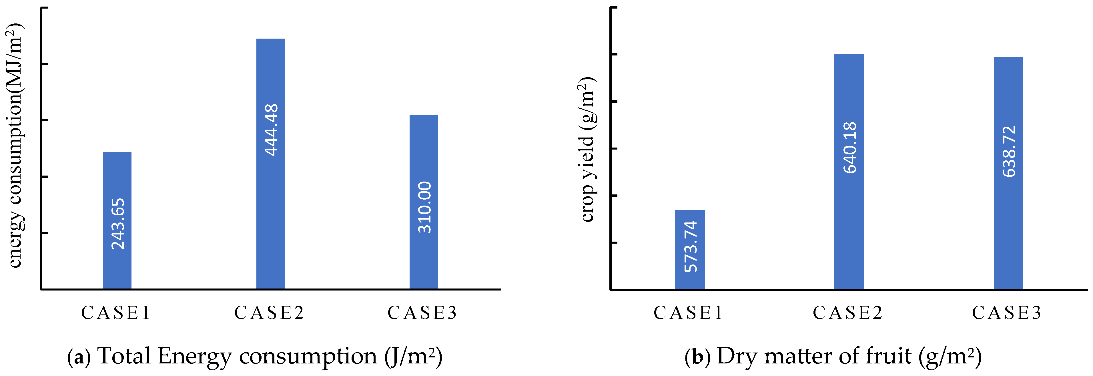
If the decision space of the optimisation problem is defined as ${\overline{T}}_{overall}\times {\overrightarrow{CO}}_{2,air}^{overall}\in [12,19]\times [450,1000]$, then a 20 × 20 grid division of the decision space yields a grid surface with respect to the total energy consumption of the heating, the total CO₂ increase, and the crop yield, as depicted in Figure 11.

The grid surface with respect to the crop yield and energy consumption accurately reflects the effects of the different matchings of the different setpoints on crop yield and energy consumption and can be regarded as a surrogate model of the crop yield and energy consumption. Therefore, the optimal solution can be directly searched on the grid surface, which can avoid the need to simulate the overall control process of the greenhouse climate for each candidate solution. Thus, the computation of the objective functions can be greatly reduced. In this study, the proposed global optimisation of the greenhouse climate setpoint can be considered a special surrogate-based optimisation. Additionally, as the energy consumption is estimated by directly integrating the control inputs, and any solution of the optimisation problem represents a full greenhouse climate control process, the optimisation process considers the effect of the control performance on the optimal solutions, which makes it more reliable in practice.

3. Results

3.1. Validation and Performance Analysis of Model-Based Interpolation Control Method

To validate the control performance of the proposed control method, the historical weather data from the Shanghai area on 11–20 September and 21–30 December 2014 were used to drive the model to simulate greenhouse climate control of ten consecutive days. During 11–20 September 2014, the outdoor temperatures were high. As a result, the indoor temperature setpoint could be aligned with outdoor conditions. However, the indoor temperature may be excessively high due to the strong solar radiation during the day, thereby the wet curtain must be turned on to cool the greenhouse. Conversely, during 21–30 December 2014, the cold weather requires the activation of the heating system to maintain an optimal growth environment. Both operations consume significant amounts of energy. In this simulation, the capacity of the fan was set at 6.6 W·m⁻², while the heating power was set at 300 W·m⁻².

Figure 12 illustrates the control results of the temperature under the cold weather conditions from 21–30 December 2014. The nighttime temperature setpoint is 12 °C, while the daytime setpoint is determined by Equation (11). From Figure 13, it can be observed that the control strategy of the heating without correction results in a maximum error of 4.4 °C and the root mean square error of 1.78 °C. However, when the corrected control strategy is used, the maximum control error is reduced to 3.5 °C and the root mean square error is reduced to 0.67 °C. Using the feedback to correct the control strategy can effectively improve control performance. As crop growth significantly depends on the daily average indoor temperatures, as shown in Figure 14, the corrected heating controls ensure that the control error of the daily average temperatures is less than 0.5 °C, while the original control strategy results in a maximum control error of the daily average temperature of 1.6 °C, and an average control error of 0.8 °C. As can be seen from Figure 12 and Figure 13, the original control strategy of the heating does not have the ability to raise the temperature on cold days, which means that the energy consumption of the corrected control strategy is higher than that of the original control strategy, as shown in Figure 14.

During 11–20 September 2014, the weather was warm, and the outdoor temperature usually changed from 15 to 27 °C. Such a temperature is beneficial to crop growth, and the indoor temperature setpoint usually follows the outdoor temperature. The main regulation operation is the ventilation. However, during the day, the solar radiation may be strong, and a pad-and-fan system is required to be turned on to cool the greenhouse. Figure 15 illustrates the control results of two control strategies of a pad-and-fan system. One strategy is obtained by directly interpolating through the control rules, while the other is the corrected control strategy.

It is observed that the control performance of the corrected control strategy is better than that of the original control strategy. The maximum control error of the original correction strategy is 7.9 °C, and the corresponding root mean square error is 1.79 °C, while the corrected control strategy has a maximum control error of 4.7 °C and a root mean square error of 1.16 °C. As shown in Figure 16, during the night, both strategies achieved similar control performances. However, during the day, if the solar radiation is high, it can be observed that the control error of the original pad-fan control strategy is larger than that of the corrected pad-fan control strategy. Due to insufficient cooling, the indoor temperatures may reach the upper bound. Nevertheless, as depicted in Figure 17, the average daily temperatures of both cases are similar. The average control error of the corrected control strategy is less than 1 °C, but the energy consumption of the corrected strategy is twice that of the original control strategy, as illustrated in Figure 18.

Whether using the direct interpolation control strategy or the corrected control strategy, it is necessary to use the pad–fan system to reduce the indoor temperature, which will result in much energy consumption. Under warm weather conditions, if the outdoor temperature changes within an acceptable range, then we limit the extreme temperature rather than excessively focus on the control error. For example, the temperature range of 20–30 °C is usually suitable for tomato crops, and the transient temperature fluctuations do not significantly impact crop yield. Therefore, in most cases, we can use ventilation to cool the greenhouse instead of using the pad–fan system. Additionally, if the solar radiation is strong, the external shading can be used to reduce the indoor temperature. Figure 18 illustrates the response of the indoor temperature under weather conditions from 11–20 September 2014 when only roof windows were opened for ventilation. It can be observed that even if only the roof ventilation is operated, the control error of the indoor temperature is not more than 1.9 °C, and the root mean square error is less than 1.05 °C, while the average temperature control error is smaller, as depicted in Figure 19. From a perspective of reducing the control error and energy saving, only opening the roof window can achieve better control performance. The simulation results indicate that, under warm weather conditions, we should use ventilation operations to maintain indoor temperatures rather than use the pad-and-fan system as much as possible in the control process.

The objective of greenhouse environmental regulation is not only to minimize tracking errors, but also to reduce energy consumption and enhance crop yield. Therefore, greenhouse environmental regulation should not excessively focus on reducing the control errors, instead, it is necessary to drive the greenhouse climate into a given interval around the setpoint.

This study considers three different control strategy scenarios:

Case1: The indoor temperature is regulated by ventilation through the roof windows on warm days, while, under cold weather conditions, the heating control strategy is generated by the control interpolation surface.

Case2: The indoor temperature is regulated by ventilation through the roof windows in warm day conditions. Under cold weather conditions, it uses the corrected interpolation control strategy to generate the heating control input.

Case3: Under warm weather conditions, we use the corrected interpolation control strategy to generate control input of the pad–fan system, and when the weather is cold, we use the corrected interpolation control strategy to generate the heating control input.

The first two cases can reflect the effects of two different heating control strategies on greenhouse environmental regulation, energy consumption, and crop yield. Similarly, the first and third cases can examine the effects of ventilation and pad-and-fan cooling on setpoint tracking control performance, energy consumption, and crop yield under warm weather conditions. These comparative studies contribute to developing a more rational control strategy for the greenhouse climate.

In the simulation, the crop growth period was set to 120 days, and the TOMGRO model was utilized to simulate the crop growth. The indoor temperature setpoint follows the outdoor temperature during warm weather conditions, while the daily average temperature setpoint is set as 18 °C on cold days. The setpoint of each day was determined using Equations (10) and (11). The lower bound of the temperature is 12 °C, and the upper bound is 35 °C. Additionally, the indoor CO₂ concentration was maintained at 450 ppm. Real weather data collected from 1 September to 28 December 2014, in Shanghai, were used for the simulation. Figure 20 and Figure 21 illustrate the total energy consumption and crop yields of three control strategies, respectively.

From the simulation results, it is evident that the first control strategy has the best energy efficiency, and that the total energy consumption is 3.3 × 10⁸ (J/m²) and the crop yield is 573 (g/m²). The remaining two control strategies exhibit similar energy-saving performance, and the energy consumption is approximately 3.8 × 10⁸ (J/m²). It should be noted that the third scenario has a 9 × 10⁵ (J/m²) higher energy consumption than the second scenario, because, in Case 3, the pad-and-fan system was turned on to cool the greenhouse on warm days, but both scenarios can achieve almost the same crop yield. As illustrated in Figure 21, the difference of the energy consumption between Case 1 and the other cases began to rise from November, because the weather became cold, and energy consumption of the heating began to rise. Therefore, the key to energy-saving for greenhouse climate regulation is to reduce the energy consumption of heating. The reason that Case 1 can achieve better energy-saving performance is that the actual indoor temperature is lower than the setpoint, but the crop yield was not significantly reduced. This result indicates that the given setpoint is not optimal, and it is important to optimise the setpoint for energy-saving.

The ambient temperature is a primary environmental factor for crop growth. When the temperature fluctuates within a reasonable range, raising the temperature may not result in a significant increase in crop yield. In this case, reducing the control error is not excessively important. Excessively high temperatures can inhibit crop growth and increase energy consumption. For instance, on cold days, if the average daily temperature is at 17 °C, the energy consumption is only 3.1 × 10⁸ (J/m²), and the crop yield is 638.72 (g/m²). However, when the daily average setpoint rises to 19 °C, the energy consumption rises to 4.55 × 10⁸ (J/m²), and crop yield reduces to 447 (g/m²). Properly reducing the average temperature can achieve a lower energy consumption and a higher crop yield. For example, when the average daily temperature is set as 16 °C, the energy consumption decreases to 2.58 × 10⁸ (J/m²), and the crop yield decreases slightly to 619 (g/m²), which indicates that an optimal daily average temperature is in the neighbourhood of 17 °C. Furthermore, when comparing cases with an average daily temperature of 17 °C, and when the setpoint changes from 16 °C to 17 °C, the energy consumption rises by 20.1%, while the crop yield only rises by 3%. From an economic perspective, if considering the electric power price to be CNY 0.6 kWh⁻¹, the setpoint 16 °C is better than 17 °C.

As each estimation of the energy consumption and yield represents a complete control process of the greenhouse climate, if the greenhouse climate model is accurate, the estimated energy consumption and crop yield are also accurate. In multi-layer hierarchical optimisation proposed in previous work, as the steady-state model ignores the energy consumption of the transient process and the control error, the estimated energy consumption may have a large error. Therefore, it is difficult to ensure that the optimisation results will be optimal in practice. Figure 22 shows the globally optimal result obtained by steady-state optimisation. It can be seen from Figure 22 that the energy consumption of global optimisation under steady-state conditions is only 2.44 × 10⁸ (J/m²), but that the energy consumption of the setpoint tracking control with the same setpoint is 4.44 × 10⁸ (J/m²).

There exists a significant disparity in energy consumption between steady-state global optimisation and dynamic control. This indicates that the globally optimal setpoint obtained under steady-state conditions is not optimal in practice. However, dynamic global optimisation of energy consumption and crop yield can achieve a reliable globally optimal setpoint, because the objective estimations of the optimisation problem consider the controller performance and the energy consumption of the transient process. Figure 22 illustrates the total energy consumption and crop yield of the case when the global average temperature setpoint is set as 17 °C. In contrast to the optimal setpoint obtained under steady-state conditions, we can save 30.2% energy under dynamic conditions, which indicates the advantage of global optimisation under dynamic conditions.

If the indoor CO₂ concentration is increased from 450 ppm to 600 ppm, and the daily average temperature is maintained at 16 °C, the crop yield rises from 619 (g/m²) to 664 (g/m²) with the same energy consumption. It can be observed that the loss of crop yield due to the low temperature can be compensated by increasing the CO₂ concentration. Therefore, the regulation of indoor CO₂ concentration is important for energy saving. By using the proposed control strategy of the CO₂ concentration, the indoor CO₂ concentration can be regulated to the setpoint, as shown in Figure 23. The control results depicted in Figure 23 indicate that a good control performance of CO₂ concentration can be achieved using the control strategy presented by Equation (19). During the day, the controlled CO₂ concentration fluctuates slightly around the setpoint with a root mean square error of only 15.11 ppm.

The simulation results of the temperature and CO₂ concentration control prove that the novel control method proposed in this study can achieve the desired control performance on a large control step size. The proposed control method provides a chance to reduce the simulation time of the control process and improve the real-time performance. In this work, the simulation is performed on the platform with Windows 11, CPU intel I7-12900H, and 32G memory, and the simulation time of the overall control process with 120 days is only 13.63 s.

3.2. Global Optimisation Analysis

If we consider that the price of electricity is 0.6 CNY/kwh, the price of CO₂ is 5 CNY/kg, and the selling price of tomato (fresh weight) is 10 CNY/kg, then the optimal average setpoint of the indoor temperature is 15.85 °C, and the CO₂ concentration setpoint is 450 ppm. Accordingly, the profit is −11.2 CNY/m², which means that it is not profitable, and the CO₂ concentration is at the lower bound, which indicates that it is not reasonable to increase the CO₂ supply in this situation. If the CO₂ price can be reduced to below 3.4 CNY/kg, the production cost will be equal to the sales revenue, and the profit will be zero.

As the price of electricity is typically fixed, the profit of greenhouse crop production is primarily influenced by the selling price of agricultural products and the fluctuation of the CO₂ price. If industrial CO₂ is utilized, and the price can be reduced to 0.15 CNY/kg, then, when the sales price of the tomato (fresh weight) is 10 CNY/kg, a profit of 28.8 CNY/m² can be achieved. In this case, the optimal average CO₂ concentration is at the upper bound, and the optimal average temperature is only 13.05 °C. It can be observed that, when the price of CO₂ is low, we can increase the CO₂ concentration to promote yield as a priority, and we avoid turning on the heating as much as possible for energy saving. However, if the agricultural product price rises to 20 CNY/kg, then the profit can rise to 97.85 CNY/m², and the corresponding optimal average temperature rises to 17.25 °C. In summary, the key factors that influence global optimisation of the greenhouse environmental setpoint when considering a profitability-oriented greenhouse crop production are the selling prices of agricultural products and the CO₂ price. If the sales price of agricultural product changes from 10 to 20 CNY/kg, and the CO₂ price varies from 0.15 to 5 CNY/kg, we can mesh the profit, the optimal average setpoints of the temperature and CO₂ concentration, as shown in Figure 24.

The optimization results indicate that the optimal setpoint of greenhouse climate significantly depends on the prices of energy and agricultural product price. If the agricultural product price is high, the setpoints of the temperature and CO₂ concentration converge to a high level in the optimization to create a comfortable growth environment, and a high crop yield can be achieved. However, if the energy price is high, and the profit cannot be ensured, the optimization process will converge to a low setpoint, which will result in a lower crop yield.

4. Discussion

The primary objective of greenhouse crop production is to maximize economic benefits within a limited time and cost investment. Therefore, it must minimize the energy cost and maximize the crop yield. However, the energy consumption and crop yield of greenhouse crop production significantly depend on the setpoint of the greenhouse climate. Therefore, the setpoint of the greenhouse climate must be reasonably programmed. A fundamental task of greenhouse climate regulation is to ensure the safety of crop growth, i.e., if the weather is hot, it must reduce the temperature by cooling operations such as the pad-and-fan system or fogging. Conversely, when the weather is cold, the heating system must be turned on to supply extra heat. Both control operations usually consume a lot of energy. Consequently, there exists the lowest energy consumption for maintaining a fundamental growth environment.

Similarly, if the indoor CO₂ cannot be reasonably compensated when the light condition is sufficient, the indoor CO₂ concentration will be low, which inhibits photosynthesis. When the indoor CO₂ concentration is lower than the outdoor CO₂ concentration, an effective way to compensate the indoor CO₂ is to introduce the outside CO₂ by ventilation. Although such a method can provide a zero-cost CO₂ enrichment, it can also result in much heat loss when the weather is cold. Therefore, it is important to make a trade-off between ventilation operation and CO₂ injection. Such a decision usually depends on the desired CO₂ concentration setting and the price of CO₂, that is, the greenhouse climate setpoint must be optimized by maximizing financial return.

Nowadays, the most typical control strategy and setpoint optimisation approach is a class of optimal control for the greenhouse climate. For example, van Henten proposed a time-scale decomposition-based optimal control method [29], and van Beveren developed an optimal control approach based on a given minimal energy and grower-defined bounds [39], van Straten proposed a user-accepted optimal control method [40], Seginer shared a setpoint optimisation method for lettuce [22]. The basic idea of such optimal control is to optimise the control strategy and setpoint trajectory of the greenhouse climate by minimizing the net economic return of the crop production process. The optimal control problem can be solved numerically using the maximum principle of Pontryagin. According to the classical optimal control theory, if the weather can be accurately predicted at each control step, the control strategy and setpoint must be optimal. However, for a long cultivation cycle, it is hard to accurately forecast the weather at such a time scale. To deal with the uncertainty of the weather, and inspired by van Henten’s result, Xu proposed an adaptive two-timescale receding horizon optimal control [30]. If the weather can be accurately forecast, then such an optimal control approach can usually achieve a good energy-saving performance. However, the numerical solving must use a pseudo spectral knotting method to construct the trajectories of control inputs and system states. If there are a large number of collocation points, the trajectories are usually difficult to construct. For a cultivation cycle with 120 days, if the control step size is set as 15 min, it may need 11,520 collocation points for a single control or state variable, and too many constraint equations must be satisfied, which is a great challenge for the nonlinear programming algorithms. Therefore, we must face the problem of dimensionality when using such a class of optimal control methods to solve the energy-saving regulation problem of greenhouse climate.

Therefore, for a long cultivation cycle, if we want to solve the setpoint optimisation problem, we must increase the time scale of the setpoint. For example, we can consider the time scale to be 24 h, then only 120 collocation points are required. However, the above-mentioned optimal control method is no longer available. According to the inherent characteristics of the greenhouse crop production system, this work proposed a dual closed-loop control mode for greenhouse climate regulation. Different from the typical optimal control mode in which the setpoint optimisation is incorporated into an optimal control problem, the setpoint optimisation problem and setpoint tracking control problem can be separately solved on different time scales in the proposed optimisation and control framework. The outer loop mainly solves the setpoint optimisation problem by maximizing the total crop yield and minimizing the entire energy consumption of greenhouse climate regulation, and in the inner loop, the controller can drive the greenhouse climate to track the setpoint. Compared with the typical optimal control method, the proposed method can greatly alleviate the problem of dimensionality and can dynamically adjust the real-time setpoint without changing the daily average setpoint in the control process. From an engineering practice point of view, the globally optimal control performance of the proposed control and optimisation mode may be more reliable when the long-term weather has great uncertainty.

However, a crucial issue of the proposed control and optimisation mode is the accurate estimation of the energy consumption and crop yield. One effective way is to simulate the entire control process of the greenhouse climate and directly calculate energy consumption and crop yield using the obtained simulation data of the control input and greenhouse climate. The advantage of such an estimation method is that it considers the control error of the greenhouse climate, while the disadvantage is that the objective functions of the optimisation problem are excessively expensive. A way to reduce the simulation time of the control process is to increase the control step size. However, for some typical Lyapunov-based control methods, when the control step size is large, stability may not be ensured. Therefore, it is necessary to develop a novel control method that can ensure the convergence of the control process on a large control step size. However, although a correction approach was introduced to improve the performance of the derived control rules, the control error may still be large in some cases, because the control rule library cannot cover the cases that were not considered in the simulation. Essentially, if we want to further improve the performance of the control rules, then we must increase the sample size of the initial indoor and outdoor climate.

5. Conclusions

Global optimisation for a greenhouse climate setpoint must solve three key issues—to accurately simulate the greenhouse climate and growth, to reduce the simulation time of the greenhouse climate control process, and to reduce the dimension of the decision space to avoid the problem of dimensionality. To solve such problems, this work developed a greenhouse climate model with eight state variables and proposed a novel data-driven control method and surrogate-based global optimization approach. The optimisation results indicate that the optimal setpoint is significantly influenced by the fluctuations in the sales price of the agricultural product and CO₂ price. The profit of the greenhouse crop production varies greatly with the prices, which leads to a significant disparity in the optimal setpoint. When agricultural product prices are low, and CO₂ prices are high, it is unreasonable to increase the CO₂ supply in greenhouse climate control process. Therefore, it is essential to monitor and predict market prices of agricultural products and CO₂ to adjust the global online optimization of the setpoint to ensure the profitability of greenhouse crop production. The rapid and efficient control and optimisation method proposed in this paper offers an effective way to solve the global optimization problem of a greenhouse climate setpoint.

References

1. Katzin, D. Energy Saving by LED Lighting in Greenhouses: A Process-Based Modelling Approach. Ph.D. Thesis, Wageningen University, Wageningen, The Netherlands, 2021. [Google Scholar]
2. Chahidi, L.O.; Fossa, M.; Priarone, A.; Mechaqrane, A. Energy saving strategies in sustainable greenhouse cultivation in the mediterranean climate—A case study. Appl. Energy 2021, 282, 116156. [Google Scholar] [CrossRef]
3. Jiang, W.; Jin, Y.; Liu, G. Net-zero energy optimization of solar greenhouses in severe cold climate using passive insulation and photovoltaic. J. Clean. Prod. 2023, 402, 136770. [Google Scholar] [CrossRef]
4. Gorjian, S.; Calise, F.; Kant, K.; Ahamed, M.S.; Copertaro, B.; Najafi, G.; Zhang, X.X.; Aghaei, M.; Shamshiri, R.R. A review on opportunities for implementation of solar energy technologies in agricultural greenhouses. J. Clean. Prod. 2021, 285, 124807. [Google Scholar] [CrossRef]
5. Cuce, E.; Harjunowibowo, D.; Cuce, P.M. Renewable and sustainable energy saving strategies for greenhouse systems: A comprehensive review. Renew. Sustain. Energy Rev. 2016, 64, 34–59. [Google Scholar] [CrossRef]
6. Fabrizio, E. Energy reduction measures in agricultural greenhouses heating: Envelope, systems and solar energy collection. Energy Build. 2012, 53, 57–63. [Google Scholar] [CrossRef]
7. Nasrollahi, H.; Ahmadi, F.; Ebadollahi, M.; Nobar, S.N.; Amidpour, M. The greenhouse technology in different climate conditions: A comprehensive energy-saving analysis. Sustain. Energy Technol. Assess. 2021, 47, 101455. [Google Scholar] [CrossRef]
8. Zhang, M.; Yan, T.; Wang, W.; Jia, X.; Wang, J.; Klemeš, J.J. Energy-saving design and control strategy towards modern sustainable greenhouse: A review. Renew. Sustain. Energy Rev. 2022, 164, 112602. [Google Scholar] [CrossRef]
9. Tong, G.; Chen, Q.; Xu, H. Passive solar energy utilization: A review of envelope material selection for Chinese solar greenhouses. Sustain. Energy Technol. Assess. 2022, 50, 101833. [Google Scholar] [CrossRef]
10. Azaza, M.; Tanougast, C.; Fabrizio, E.; Mami, A. Smart greenhouse fuzzy logic based control system enhanced with wireless data monitoring. ISA (Instrum. Soc. Am.) Trans. 2016, 61, 297–307. [Google Scholar] [CrossRef]
11. Shen, Y.; Wei, R.; Xu, L. Energy consumption prediction of a greenhouse and optimization of daily average temperature. Energies 2018, 11, 65. [Google Scholar] [CrossRef]
12. Mahmood, F.; Govindan, R.; Bermak, A.; Yang, D.; Khadra, C.; Al-Ansari, T. Energy utilization assessment of a semi-closed greenhouse using data-driven model predictive control. J. Clean. Prod. 2021, 324, 129172. [Google Scholar] [CrossRef]
13. Ajagekar, A.; Decardi-Nelson, B.; You, F. Energy management for demand response in networked greenhouses with multi-agent deep reinforcement learning. Appl. Energy 2024, 355, 122349. [Google Scholar] [CrossRef]
14. Ajagekar, A.; Mattson, N.S.; You, F. Energy-efficient AI-based Control of Semi-closed Greenhouses Leveraging Robust Optimisation in Deep Reinforcement Learning. Adv. Appl. Energy 2023, 9, 100119. [Google Scholar] [CrossRef]
15. Ajagekar, A.; You, F. Deep Reinforcement Learning Based Automatic Control in Semi-Closed Greenhouse Systems. IFAC PapersOnLine 2022, 55, 406–411. [Google Scholar] [CrossRef]
16. Troncoso-García, A.R.; Britob, I.S.; Troncoso, A.; Martínez-Álvarez, F. Explainable hybrid deep learning and Coronavirus Optimisation Algorithm for improving evapotranspiration forecasting. Comput. Electron. Agric. 2023, 215, 108387. [Google Scholar] [CrossRef]
17. Zhou, X.; Liu, Q.; Katzin, D.; Qian, T.; Heuvelink, E.; Marcelis Leo, F.M. Boosting the prediction accuracy of a process-based greenhouse climate-tomato production model by particle filtering and deep learning. Comput. Electron. Agric. 2023, 211, 107980. [Google Scholar] [CrossRef]
18. Xu, Z.; Lu, J.; Xing, S. Thermal performance of greenhouse heating with loop heat pipe solar collector and ground source heat pump. Results Eng. 2022, 15, 100626. [Google Scholar] [CrossRef]
19. Iqbal, Z.; Islam, N.; Kabir, S.N.; Gulandaz, A.; Reza, N.; Jang, S.-H.; Chung, S.-O. Comparison of heating modules for suspension-type multipoint temperature variability management in smart greenhouses. Smart Agric. Technol. 2023, 5, 100296. [Google Scholar] [CrossRef]
20. Yang, X.; Sun, D.; Li, J.; Yu, C.; Deng, Y.; Yu, B. Demonstration study on ground source heat pump heating system with solar thermal energy storage for greenhouse heating. J. Energy Storage 2022, 54, 105298. [Google Scholar] [CrossRef]
21. Katzin, D.; Marcelis Leo, F.M.; van Henten Eldert, J.; van Mourik, S. Heating greenhouses by light: A novel concept for intensive greenhouse production. Biosyst. Eng. 2023, 230, 242–276. [Google Scholar] [CrossRef]
22. Seginer, I.; Shina, G.; Albright, L.D.; Marsh, L.S. Optimal temperature setpoints for greenhouse lettuce. J. Agric. Eng. Res. 1991, 49, 209–226. [Google Scholar] [CrossRef]
23. Sigrimis, N.; Ferentinos, K.P.; Arvanitis, K.G.; Anastasiou, A. A Comparison of Optimal Greenhouse Heating Setpoint Generation Algorithms for Energy Conservation. IFAC Proc. Vol. 2001, 34, 61–66. [Google Scholar] [CrossRef]
24. Chen, J.; Yang, J.; Zhao, J.; Xu, F.; Shen, Z.; Zhang, L. Energy demand forecasting of the greenhouses using nonlinear models based on model optimized prediction method. Neurocomputing 2016, 174, 1087–1100. [Google Scholar] [CrossRef]
25. HEUVELINK, E. Evaluation of a dynamic simulation model for tomato crop growth and development. Ann. Bot. 1999, 83, 413–422. [Google Scholar] [CrossRef]
26. Golzar, F.; Heeren, N.; Hellweg, S.; Roshandel, R. A novel integrated framework to evaluate greenhouse energy demand and crop yield production. Renew. Sustain. Energy Rev. 2018, 96, 487–501. [Google Scholar] [CrossRef]
27. Su, Y.; Xu, L.; Goodman, E.D. Multi-layer hierarchical optimisation of greenhouse climate setpoints for energy conservation and improvement of crop yield. Biosyst. Eng. 2021, 205, 212–233. [Google Scholar] [CrossRef]
28. Su, Y.; Xu, L. Setpoint decision support strategy and adaptive hybrid control of greenhouse climate: A simulation study. Int. J. Control Autom. Syst. 2022, 20, 3740–3758. [Google Scholar] [CrossRef]
29. van Henten, E.J.; Bontsem, J. Time-scale decomposition of an optimal control problem in greenhouse climate management. Control Eng. Pract. 2009, 17, 88–96. [Google Scholar] [CrossRef]
30. Xu, D.; Du, S.; van Willigenburg, G. Adaptive two time-scale receding horizon optimal control for greenhouse lettuce cultivation. Comput. Electron. Agric. 2018, 146, 93–103. [Google Scholar] [CrossRef]
31. Xu, D.; Du, S.; van Willigenburg, G. Double closed-loop optimal control of greenhouse cultivation. Control Eng. Pract. 2019, 85, 90–99. [Google Scholar] [CrossRef]
32. Xu, D.; Li, Y.; Dai, A.; Zhao, S.; Song, W. Model-based quantitative analysis in two-time-scale decomposed on–off optimal control of greenhouse cultivation. Inf. Process. Agric. 2024, 11, 488–498. [Google Scholar] [CrossRef]
33. Katzin, D.; van Henten, E.J.; van Mourik, S. Process-based greenhouse climate models: Genealogy, current status, and future directions. Agric. Syst. 2022, 198, 103388. [Google Scholar] [CrossRef]
34. van Ooteghem, R.J.C. Optimal Control Design for a Solar Greenhouse. Ph.D. Thesis, Wageningen University, Wageningen, The Netherlands, 2007. [Google Scholar]
35. Vanthoor, B. A Model Based Greenhouse Design Method. Ph.D. Thesis, Wageningen University, Wageningen, The Netherlands, 2011. [Google Scholar]
36. De Zwart, H.F. Analyzing Energy-Saving Options in Greenhouse Cultivation Using a Simulation Model. Ph.D. Thesis, Landbouw Universiteit, Wageningen, The Netherlands, 1996. [Google Scholar]
37. Jones, J.W.; Kenig, A.; Vallejos, C.E. Reduced state variable tomato growth model. Trans. ASAE 1999, 42, 255–265. [Google Scholar] [CrossRef]
38. Kaneko, T.; Nomurab, K.; Yasutake, D.; Iwao, T.; Okayasu, T.; Ozaki, Y.; Mori, M.; Hirota, T.; Kitano, M. A canopy photosynthesis model based on a highly generalizable artificial neural network incorporated with a mechanistic understanding of single-leaf photosynthesis. Agric. For. Meteorol. 2022, 323, 109036. [Google Scholar] [CrossRef]
39. van Beveren, P.J.M.; Bontsema, J.; van Straten, G.; van Henten, E.J. Optimal control of greenhouse climate using minimal energy and grower defined bounds. Appl. Energy 2015, 159, 509–519. [Google Scholar] [CrossRef]
40. van Straten, G.; Challa, H.; Buwald, F. Towards user accepted optimal control of greenhouse climate. Comput. Electron. Agric. 2000, 26, 221–238. [Google Scholar] [CrossRef]
Figure 1. Dual closed-loop control system of greenhouse climate and crop growth, where T a i r , w a i r , C O 2 , a i r are the temperature, humidity and CO2 concentration inside the greenhouse, respectively, and T o u t , w o u t , C O 2 , o u t , V w i n d and I g l o b are the temperature, humidity, CO2 concentration, wind speed and solar radiation outside greenhouse, respectively. The superscript * denotes the setpoint of greenhouse climate.
Agriculture 15 00939 g001
Figure 2. The methodological framework of the proposed method.
Agriculture 15 00939 g002
Figure 3. Optimal photosynthetic temperature compensation during the day.
Agriculture 15 00939 g003
Figure 4. Response of photosynthesis rate on light quantum flux density and temperature.
Agriculture 15 00939 g004
Figure 5. Daily temperature setpoint trajectory.
Agriculture 15 00939 g005
Figure 6. CO2 concentration setpoint trajectory.
Agriculture 15 00939 g006
Figure 7. Construction process of control rule library. The superscript * represents the setpoint of a variable.
Agriculture 15 00939 g007
Figure 8. Control interpolation surface of heating during night.
Agriculture 15 00939 g008
Figure 9. Interpolation of pad control during night.
Agriculture 15 00939 g009
Figure 10. Flowchart of accumulated temperature allocation strategy and its demonstration.
Agriculture 15 00939 g010
Figure 11. The total energy consumption, CO2 consumption and crop yield with respect to setpoints.
Agriculture 15 00939 g011
Figure 12. Control simulation of the temperature inside the greenhouse with two different heating control strategies under cold weather conditions. One is the corrected heating control strategy based on Equations (9)~(17), the other is the original heating control strategy calculated by the interpolation surface.
Agriculture 15 00939 g012
Figure 13. Daily mean temperature inside the greenhouse obtained by the two heating control strategies. The maximum error (ME) and the root mean square error (RSME) of the daily mean temperature obtained by the corrected Uhot are 0.3467 °C and 0.2615 °C, respectively. While using the original Uhot, the ME and RSME are 1.730 °C and 0.925 °C, respectively.
Agriculture 15 00939 g013
Figure 14. Daily energy consumptions of the two heating control strategies.
Agriculture 15 00939 g014
Figure 15. The indoor temperatures with different control strategies Upad of the pad and fan.
Agriculture 15 00939 g015
Figure 16. Daily mean temperatures obtained by different control strategies using the Upad of the pad–fan system.
Agriculture 15 00939 g016
Figure 17. Daily energy consumption of the pad–fan system with different Upad control strategies.
Agriculture 15 00939 g017
Figure 18. The indoor temperatures controlled by roof ventilation.
Agriculture 15 00939 g018
Figure 19. Daily mean temperature obtained using only roof ventilation.
Agriculture 15 00939 g019
Figure 20. Dry matter of fruit under different control strategies.
Agriculture 15 00939 g020
Figure 21. Total energy consumption under different control strategies.
Agriculture 15 00939 g021
Figure 22. Optimal energy consumption and crop yield under steady-state condition and dynamic condition. CASE1 represents steady-state optimisation results, CASE2 shows the results of the setpoint control with the setpoint obtained under steady-state condition, and CASE3 denotes the optimisation results with dynamic model.
Agriculture 15 00939 g022
Figure 23. Controlled CO2 concentration inside the greenhouse using the proposed control strategy.
Agriculture 15 00939 g023
Figure 24. Distribution of profit, optimal mean setpoints of temperature and CO2 concentration with respect to the prices of CO2 and crop.
Agriculture 15 00939 g024