Neuro-Fuzzy System to Predict Timely Harvest in Stevia Crops

Abstract

Agriculture is essential for food production and raw materials. A key aspect of this sector is harvest, the stage at which the commercial part of the plant is separated. Timely harvesting minimizes post-harvest losses, preserves product quality, and optimizes production processes. Globally, a substantial amount of food is wasted, impacting food security and natural resources. To address this problem, an Adaptive Neuro-Fuzzy Inference System was developed to predict timely harvesting in crops. Stevia, a native plant from Brazil and Paraguay, with an annual production of 100,000 to 200,000 tons and a market of 400 million dollars, is the focus of this study. The system considers soil pH, Brix Degrees, and leaf colorimetry as inputs. The output is binary: 1 indicates timely harvest and 0 indicates no timely harvest. To assess its performance, Leave-One-Out Cross-Validation was used, obtaining an $r^2$ of 0.99965 and an Absolute Residual Error of 0.00064305, demonstrating its accuracy and robustness. In addition, an interactive application that allows farmers to evaluate crop status and optimize decision-making was developed.

1. Introduction

Agriculture plays a crucial role in food production [1], serving as an essential activity for the economy of many developing countries, where it represents the core of export revenues and rural development. Among the critical phases of agricultural production, harvesting is the stage in which the commercially valuable portions of plants are collected. This process involves separating the commercial plant parts from the parent plant at the precise moment when the nutrients have fully developed and the edible fractions have reached the appropriate degree of maturity for subsequent processing [2,3]. Ensuring a timely harvest (TH) is essential for minimizing food waste, reducing economic losses, and preserving crop quality and nutritional value [4,5]. Approximately one-third of globally produced food is wasted, with improper harvesting contributing significantly to this issue. Optimizing harvest timing ensures crops are collected at peak maturity, maximizing yield, freshness, and storage capacity [6,7]. Harvesting too early results in underdeveloped crops with suboptimal size, shape, and weight, while late harvesting increases susceptibility to fungal spoilage, flavor deterioration, and premature fruit drop, reducing final yield [6]. Proper harvest timing and methodology are crucial for maintaining both internal and external quality, ensuring efficient crop management [8].

The appropriate time to harvest crops depends on the type of crop and its degree of maturity. Usually, this is determined by monitoring factors such as crop appearance, seed color, moisture content, and time since sowing [9,10]. The most common practices for evaluating the optimum stage of maturity and the right harvest time are based on different parameters. Among the different approaches used for this purpose are observation, texture, aroma, and biochemical and morphological changes of crops [6], as well as the expert judgment of producers and farmers.

Traditional agricultural methods, such as determining optimal harvest time, remain rudimentary, limiting efficiency. Precision Agriculture (PA) uses specialized tools to collect, process, and analyze diverse data, optimizing farming operations to improve crop quality and minimize resource use [11,12,13]. Artificial Intelligence (AI) further enhances agricultural efficiency, allowing for more precise management of plants, pests, and diseases [14]. AI applications in agriculture optimize harvesting, soil monitoring, data analysis, and food supply chains, improving productivity while reducing resource consumption, time, and costs [15,16]. A key aspect of AI is the use of hybrid techniques, which involve the combination of two or more AI methodologies, such as Neuro-Fuzzy Systems (NFSs).

An Adaptive Neuro-Fuzzy Inference System (ANFIS) is a type of NFS that adapts the rule base of a Takagi–Sugeno–Kang (TSK) Fuzzy Inference System (FIS). It employs two optimization methods for training, backpropagation and least mean squares, which adjust key parameters [17], such as the type and number of Membership Functions (MFs). Grid partitioning enhances ANFIS performance for systems with up to five variables [18], which is a characteristic relevant to this study. ANFIS has been widely used in agriculture, demonstrating its effectiveness in minimizing material, cost, time, resource, and labor losses, as shown in studies such as [19,20,21]. NFS represents a powerful tool for crop optimization and PA management.

A crop of great importance today and a member of the Asteraceae family is Stevia Rebaudiana, a high-value plant native to Brazil and Paraguay. Harvested 75–90 days after sowing [22], it is rich in protein, fiber, minerals, vitamins, and phenolic acids [23]. Its sweetness surpasses that of common sugar by 300–450 times, with a 2.62 ft plant yielding about 70 g of dehydrated leaves. Global production ranges from 100,000 to 200,000 tons annually, valued at 400 million. China dominates with 75% production, followed by Paraguay (8%), Brazil, Colombia, and Kenya. Recent expansions include Vietnam and Mexico [24]. In Mexico, the Instituto Nacional de Investigaciones Forestales, Agrícolas y Pecuarias (INIFAP) introduced Stevia to assess its adaptation, initiating production in 2010. By 2012, the Servicio de Información Agroalimentaria y Pesquera (SIAP), reported significant national figures. Colima is one of the first states in Mexico where Stevia was cultivated, a region with favorable agroclimatic conditions for its development [24,25,26].

Ensuring Stevia crop quality and productivity requires understanding critical factors influencing its conservation. Among these, soil pH and Brix Degrees (BDs) are primary indicators of plant health [27]. Additionally, leaf colorimetry serves as a key visual marker of physiological changes, aiding in the detection of nutrient deficiencies and disease. All three indicators collectively determine whether the crop has reached its peak maturity for harvesting.

Soil pH directly affects agricultural productivity, influencing nutrient solubility, crop yield, and microbial interactions. Most crops thrive in a pH range of 6 to 7, where nutrient availability is optimal, while extreme acidity (<5) or alkalinity (>7) severely limits plant growth and soil fertility [28,29,30].

BD is a key indicator of crop quality, measuring soluble solids that determine a product’s potential sweetness. BD is a critical parameter across the agricultural value chain, affecting product sweetness and market valuation. It is commonly measured using a refractometer, which utilizes specific gravity and density for precise readings [31,32].

Leaf color is an essential indicator of crop health and nutrient status. Deficiencies in key elements such as iron, magnesium, nitrogen (N), phosphorus (P), and potassium (K), collectively known as NPK, cause imbalances in the crop, which is reflected in changes in leaf color, indicating plant health problems [33,34,35,36]. Monitoring these variations enables the early detection of imbalances, optimizing crop management strategies. The appearance of crop leaves, particularly changes in color, serves as a visible indicator of nutrient imbalance. NPK deficiencies, in particular, are associated with reduced chlorophyll content, which affects both leaf coloration and overall condition [37].

The main objective of this study is to develop a predictive system based on ANFIS for determining TH in Stevia crops. The model integrates pH, BD, and leaf colorimetry as independent variables, given their significant role in nutrient availability and crop maturity assessment. The central hypothesis is that an ANFIS model trained on these indicators can reliably predict whether a Stevia crop is ready for harvest. The specific objectives of this study are as follows:

• The development of an ANFIS-based predictive system capable of classifying Stevia crops as ready for harvest (TH = 1) or not (TH = 0) using three key agronomic indicators: soil pH, Brix Degrees, and leaf colorimetry.
• The implementation of a feature extraction process for leaf colorimetry, converting leaf color into numerical values to ensure compatibility with ANFIS-based inference.
• The evaluation of the accuracy and generalization performance of the model using Absolute Residual (AR) as an error metric and Leave-One-Out Cross-Validation (LOOCV) to assess robustness.
• The comparison of the proposed model with different dataset sizes, incorporating synthetic data augmentation (1000 and 10,000 samples) to analyze its scalability and adaptability.

By fulfilling these objectives, this study contributes to data-driven decision-making in Stevia cultivation, enabling more precise and efficient harvest scheduling based on measurable agronomic indicators.

2. Materials and Methods

2.1. Data Collection and Experimental Setup

Stevia plants were used in this study to collect data for three key agronomic indicators: soil pH, BD, and leaf colorimetry. Additionally, images of the crops were captured and processed to extract numerical features, as the ANFIS model requires numerical input values. All plants were cultivated under controlled conditions, following standardized agricultural practices to ensure uniform growth and development.

The study was conducted at Rancho Tajeli, located in El Trapiche, in the southern region of the municipality of Cuauhtémoc, in the state of Colima, Mexico. The area is characterized by a warm and dry climate, with temperatures ranging from 17 °C to 31 °C, and fertile soil conditions favorable for Stevia cultivation.

The experiment focused on a sample of four rows of Stevia crops, totaling 150 plants. Field data were collected periodically, with special attention given to days close to the expected harvest window. Measurements were taken when the plants were between 80 and 90 days post-sowing, ensuring that the recorded values corresponded to crops likely to be at an optimal harvest stage.

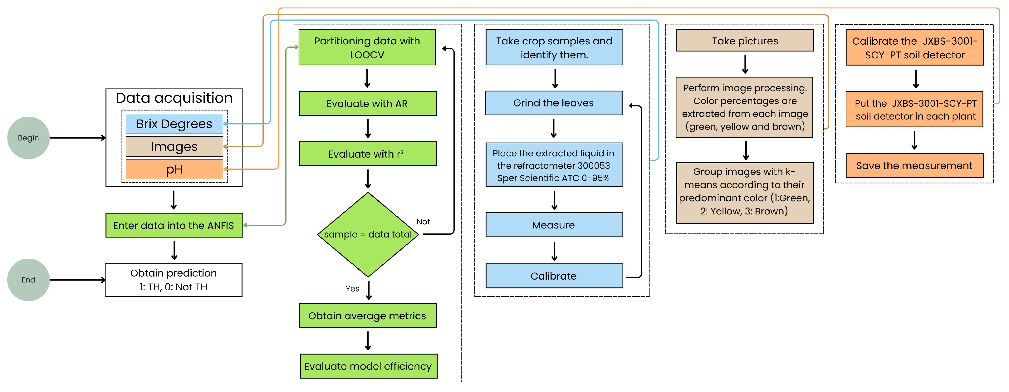
The proposed solution implements an NFS based on ANFIS architecture, combined with the grid partition method. As noted in Section 1, ANFIS is particularly effective when dealing with five or fewer independent variables. In this study, three variables were selected: soil pH, plant BD, and leaf colorimetry. These values were introduced into the NFS, which processed them through a combination of fuzzy inference rules and adaptive learning mechanisms inherent to ANFIS.

Based on the input data, the system evaluated the current crop conditions and produced a binary output for the dependent variable: 1 indicating that the crop is ready for TH, and 0 indicating that it is not. The FIS was structured using MFs and a rule base informed by agricultural expert knowledge, allowing the system to accurately classify harvest readiness based on observed crop conditions.

The overall methodology followed in this study is depicted in Figure 1.

2.2. Dataset Structure and Variables

This section describes the data collection process for each of the three independent variables used per crop sample. Section 2.2.1 details the image acquisition procedure, including the environmental setup and controlled conditions under which the photographs were taken. It also explains the image processing method used to extract color percentages (green, yellow, and brown), followed by the clustering process, in which images were grouped based on their predominant color using the k-means algorithm. Section 2.2.2 describes the soil pH data collection, including the measuring instrument employed and the protocol followed. Finally, Section 2.2.3 outlines the procedure for collecting BD data, including details of the refractometer used and the calibration process performed between each measurement.

The dataset consists of 150 samples for each of the three input variables:

• Input cluster: Value obtained after processing an image to extract color percentages. The image was then assigned to a cluster using the k-means algorithm based on the predominant color.
• Input pH: Soil pH values collected from the study area.
• Input -BD: BD values obtained from leaf samples of Stevia plants.

2.2.1. Leaf Colorimetry Feature Extraction for Cluster-Based Classification

Data acquisition was conducted in two sessions, both carried out during daytime hours, from 10:00 a.m. to 2:00 p.m. The first session took place on 25 April 2024 (70 days post-sowing), when the crops had already reached an optimal BD level for harvest. This determination was made based on the expert judgment of farmers at Rancho Tajeli, who typically harvest Stevia plants between 70 and 90 days after sowing, depending on crop development. To assess suitability for collection, they use an analog refractometer to measure the BD. Moreover, the literature [23] supports this timing, indicating that Stevia is generally harvested between 70 and 95 days after planting.

The second session was conducted on 23 May 2024 (98 days post-sowing), as the ranch farmers decided to leave some crops in the field to assess whether they could achieve a higher BD level. During this additional period, the crops continued to be carefully maintained under the same agronomic practices. Thus, the selected sampling dates are aligned with both local agronomic practices and scientific evidence on the crop’s optimal harvest timing.

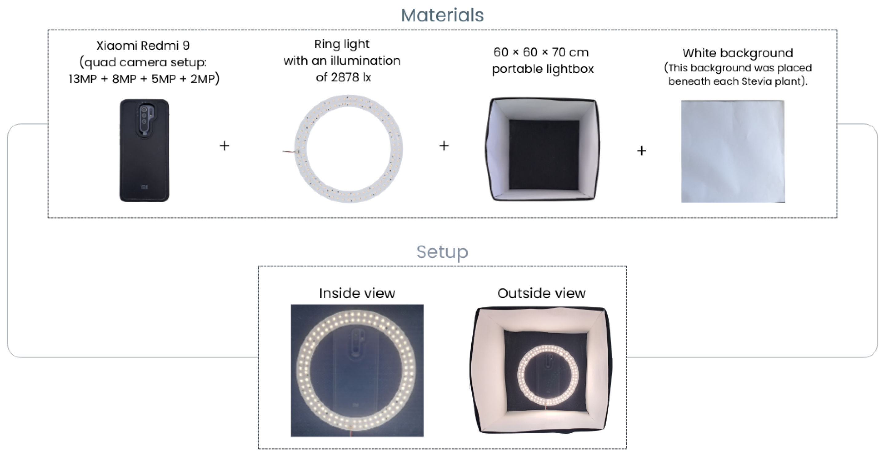
To ensure high-quality and consistent image capture, 150 images of Stevia crops were taken in a controlled environment using a 60 × 60 × 70 cm portable lightbox. A ceiling-mounted ring light provided uniform illumination at 2878 lux (symbol: lx), preventing shadows or variations in natural light that could interfere with the colorimetric analysis. The images were captured using a Xiaomi Redmi 9 smartphone (quad camera setup: 13 MP + 8 MP + 5 MP + 2 MP), which was positioned 30 cm above the lightbox opening at a 90-degree angle, ensuring a consistent height and angle across all samples.

Light levels were precisely measured using an LX1330B digital luxmeter, which has a 0 to 200,000 lx range and 0.1 lx resolution. This ensured stable lighting conditions and minimized variability due to external factors. Additionally, environmental noise was reduced to ensure that differences in the images were due to the plant’s state rather than uncontrolled external influences. The camera setup is shown in Figure 2.

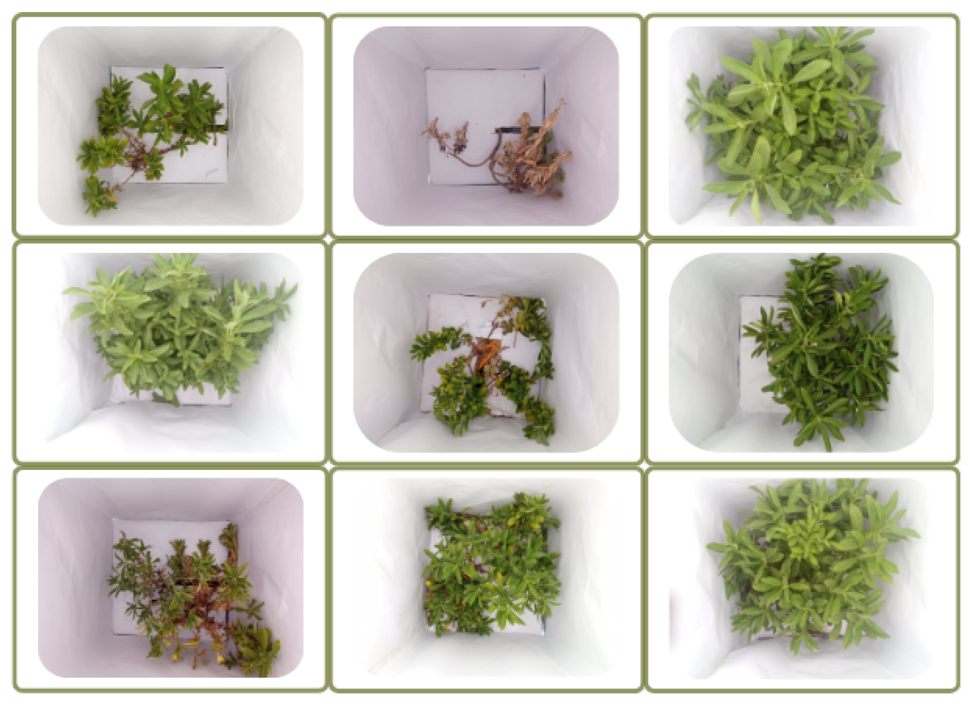
The images revealed that the plants were predominantly green, with some shades of brown and yellow, confirming that P deficiency was not present. Figure 3 illustrates a subset of the dataset images used in this study.

Furthermore,

Table 1. Nutritional indicators in plants.

Leaf Color	Indicator
Yellow	N deficiency
Purple or red	P deficiency
Brown	K deficiency
Green	Balance in NPK macronutrients

summarizes how leaf color can be indicative of specific nutrient deficiencies: yellow shades suggest N deficiency, purple or red indicate P deficiency, and brown shades reflect K deficiency. In contrast, a completely green leaf in both early and late growth stages suggests an adequate macronutrient balance [37].

By integrating a controlled environment, standardized lighting, a strategically positioned camera, and precise luxmeter readings, the methodology ensured optimal conditions for obtaining accurate and high-quality images for this study.

One of the common challenges in color-based analysis is the influence of variations in lighting conditions and camera positioning. However, in this study, these factors were carefully controlled to ensure consistency across all image acquisitions. The use of a portable lightbox with a ceiling-mounted ring light (2878 lx) provided a uniform and stable illumination, eliminating potential shadows or natural light variations that could affect color segmentation. Additionally, the fixed camera setup (30 cm height, 90-degree angle) ensured a constant capture perspective, minimizing distortions or inconsistencies. These measures significantly reduced the impact of external variables on the Hue, Saturation, and Value (HSV)-based analysis, allowing for a more reliable assessment of color distribution in the crops.

The HSV color model was used to analyze the color distribution in each image:

• H: Represents the dominant color, ranging from 0° to 360°, mapped to [0, 1] in MATLAB R2024b
• S: Indicates color purity, with values ranging from 0 to 1.
• V: Represents brightness or intensity, also within the [0, 1] range.

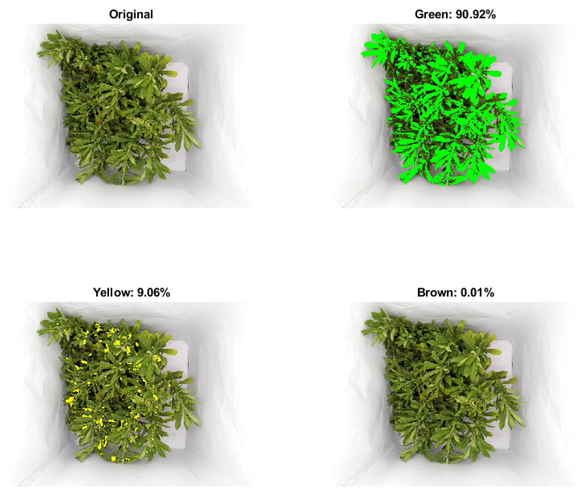
Each image was converted from the Red, Green, Blue (known as RGB) model to HSV, allowing for pixel classification into three primary categories: green, yellow, and brown, which are the predominant colors in crop leaves. One of the key advantages of the HSV model is that H remains independent of brightness and saturation, facilitating segmentation based purely on color.

For each color range, Binary Masks (BMs) were generated. A BM is a matrix of the same size as the original image, where each pixel is classified based on predefined color thresholds.

The BMs identify pixels that match the predefined color criteria. Additionally, the proportion of pixels corresponding to each H is calculated and normalized relative to the total number of classified pixels, ensuring that the total percentage sums to 100%. Figure 4 illustrates the application of BMs to one of the dataset images.

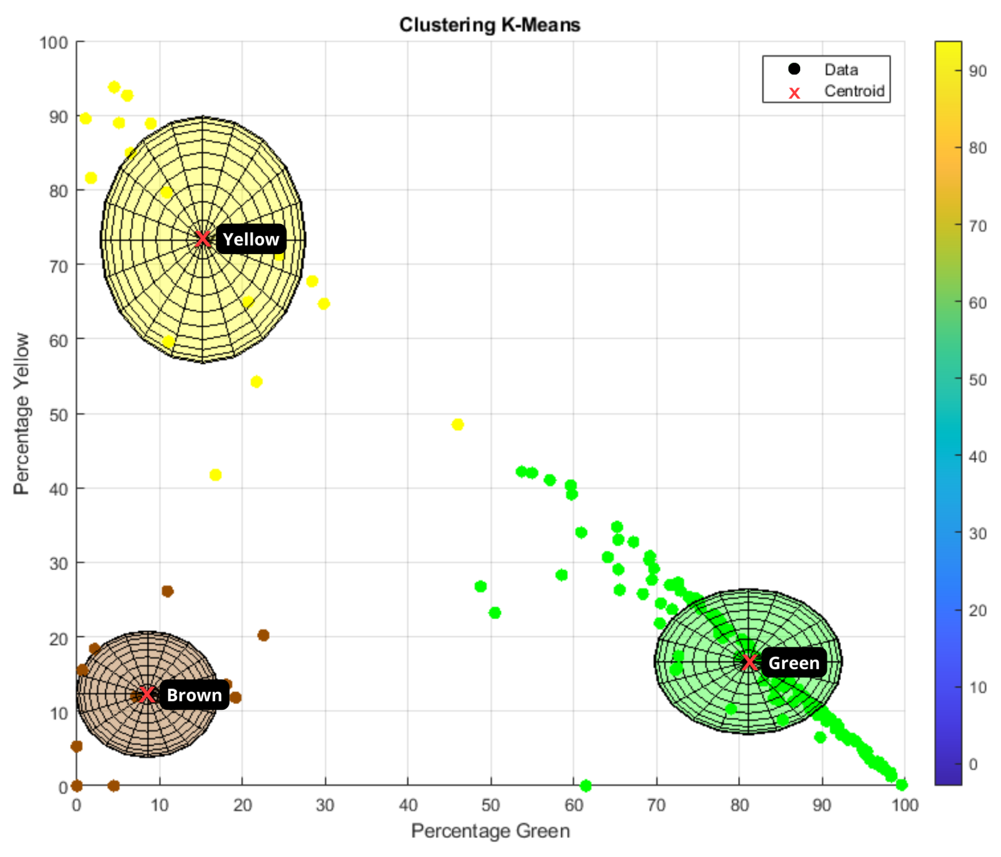
After processing the images with BMs and knowing the percentage of each color, the k-means algorithm was applied, which is an unsupervised learning method used to solve grouping or clustering problems. The main objective of this algorithm is to divide a dataset into ‘k’ groups or clusters based on the similarity of the data. The first step performed in k-means is to choose ‘k’ initial centroids; then, for each point in the dataset, the Euclidean distance with respect to each of the centroids is calculated, and the point data are assigned to the cluster whose centroid is closest. K-means has advantages such as simplicity, speed, and scalability, and has been used in works such as [38,39,40].

K-means works on the dataset with percentages of each color (green, yellow, and brown) per image and, depending on the values, assigns each image to the cluster of the predominant color. Three clusters were established, one corresponding to each color, defined as follows (

Table 2. Clusters defined.

Cluster: Color
1: Green	2: Yellow	3: Brown

).

Table 3. Clustering sample.

Image	%Green	%Yellow	%Brown	Cluster
120.jpg	99.5584	0.14344	0.29818	1
75.jpg	10.8477	79.6597	9.94261	2
76.jpg	4.44868	0	95.5513	3

presents an example of how images were grouped after processing, reflecting the overall structure of the complete dataset.

Figure 5 shows the classification of each of the images after processing and assignment to the corresponding cluster.

2.2.2. pH Acquisition

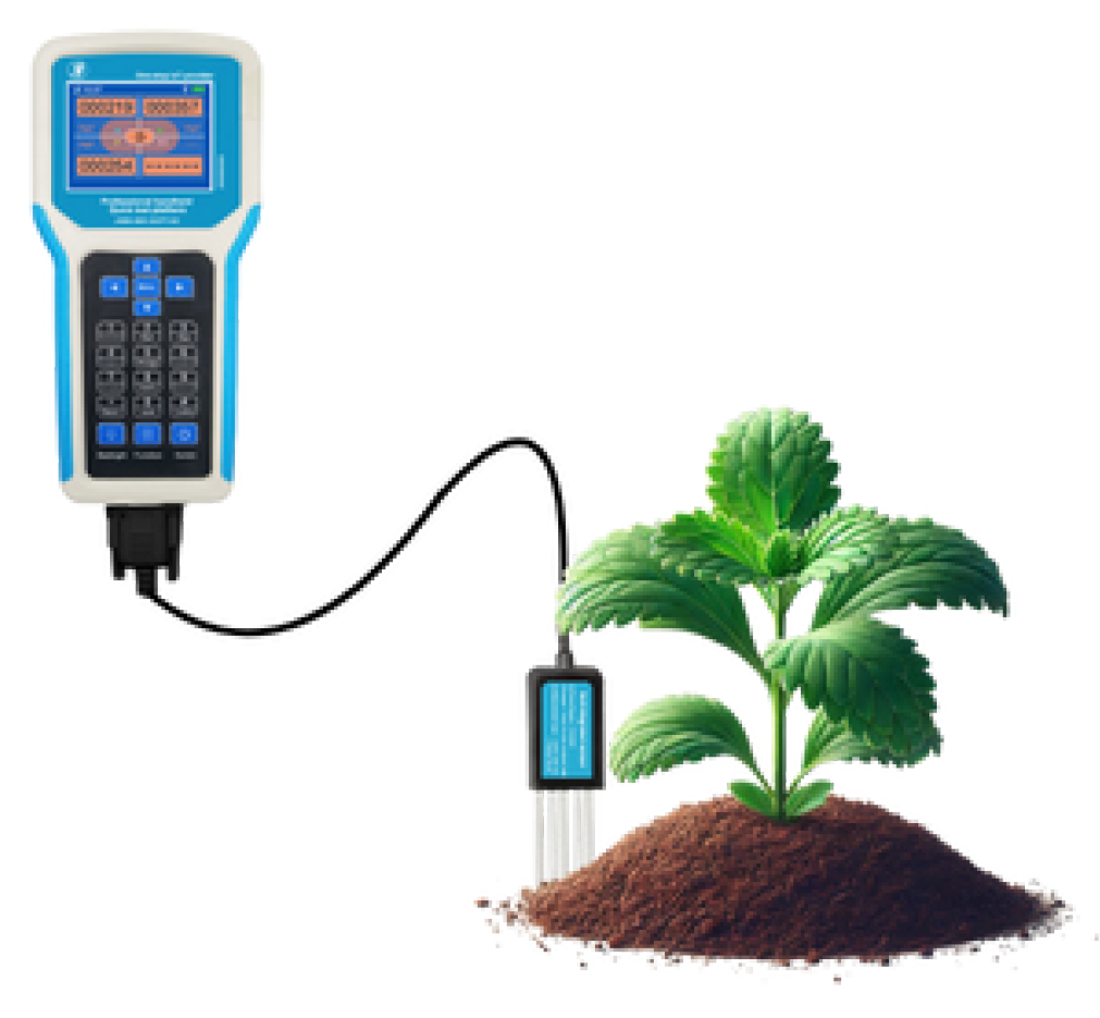
The JXBS-3001-SCY-PT portable soil detector (Jingxun Changtong Electronic Technology, Weihai, China) (Figure 6), which is designed to measure multiple soil parameters, was used to collect pH data for each of the plants. The instrument is powered by a 3.7 V power supply consumed from a lithium battery and uses the Modbus Communication Protocol over RS485 [41]. The calibration of the pH meter was performed using pH buffer solutions with pH values of 4.0, 7.0, and 10.0. The procedure was to immerse the probe of the meter in the solutions and adjust the device so that the readings coincided with the pH values of the buffer solutions. For data acquisition, the sensor was placed in the plant area for approximately 3 s.

2.2.3. Brix Degrees Acquisition

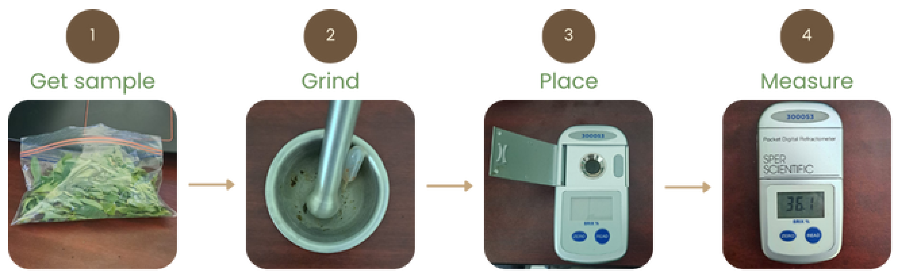
A digital refractometer model Sper Scientific (Sper Scientific, Scottsdale, AZ, USA) ATC 0–95% was used to obtain the BD data. This digital refractometer is a compact and lightweight instrument designed to accurately measure the concentration of solutions in BD, indicating the sugar content in liquids. In addition, it implements an Automatic Temperature Compensation (ATC), which automatically adjusts the readings according to the sample temperature, ensuring accurate results; its measurement range is 0 to 95% Brix, with a resolution of 0.1% Brix and an accuracy of ±0.2% Brix; the minimum sample volume required is 1 mL [42,43]. One of the features of this refractometer is the automatic calibration using distilled water. To perform the calibration, a sample of distilled water was placed on the prism of the refractometer between each measurement, and the calibration button (zero) was pressed. In this way, the instrument automatically adjusted the reading to zero.

The procedure for the extraction of the BD is shown in Figure 7.

2.3. ANFIS Modeling

As mentioned in Section 1, the ANFIS-based NFS is a hybrid model that combines the strengths of Artificial Neural Networks (ANNs) and FIS. This approach enables the modeling of complex non-linear relationships between inputs and outputs while also providing interpretability through linguistic rules. This section describes the modeling process for predicting TH, where the output is binary: 1 indicates that the crop is ready for harvest, and 0 indicates it is not. The proposed model integrates the flexibility of FIS to manage uncertainty with the learning capabilities of ANNs for parameter optimization, resulting in an accurate and adaptive predictive system.

2.3.1. Artificial Neural Network (ANN)

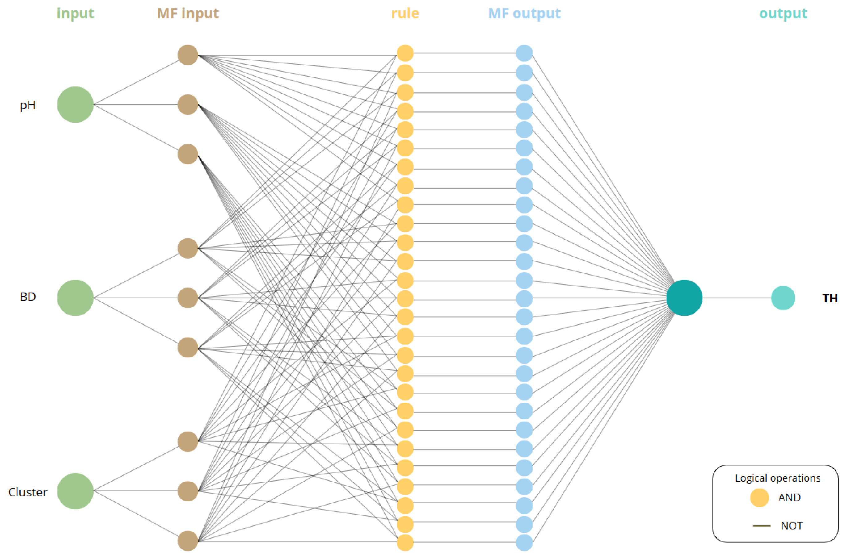
In an NFS with an ANFIS architecture, the input data are first processed by an ANN, which functions as an optimizer responsible for adjusting the parameters of a TSK-type FIS. During this stage, the model undergoes adaptive learning, where the ANN fine-tunes the weights, MFs parameters, and Fuzzy Rules (FRs). Although ANNs are highly effective in identifying optimal configurations, they are often considered “black box” models, as their internal parameter adjustments are not easily interpretable or modifiable.

The ANFIS used in this study adopts the ANN structure illustrated in Figure 8.

2.3.2. Fuzzy Inference System (FIS)

Once the ANN has adjusted the parameters, the FIS uses them to perform inference based on a set of predefined linguistic rules. In contrast to ANN, the FIS allows for a more transparent and interpretable structure, offering manageable control over the model’s logic.

The configuration of the FIS relies on three key components: the input variables, the output variable, and the set of FRs that define the decision-making process. These components are described in detail in the following subsections.

2.3.3. Input Configuration of the FIS

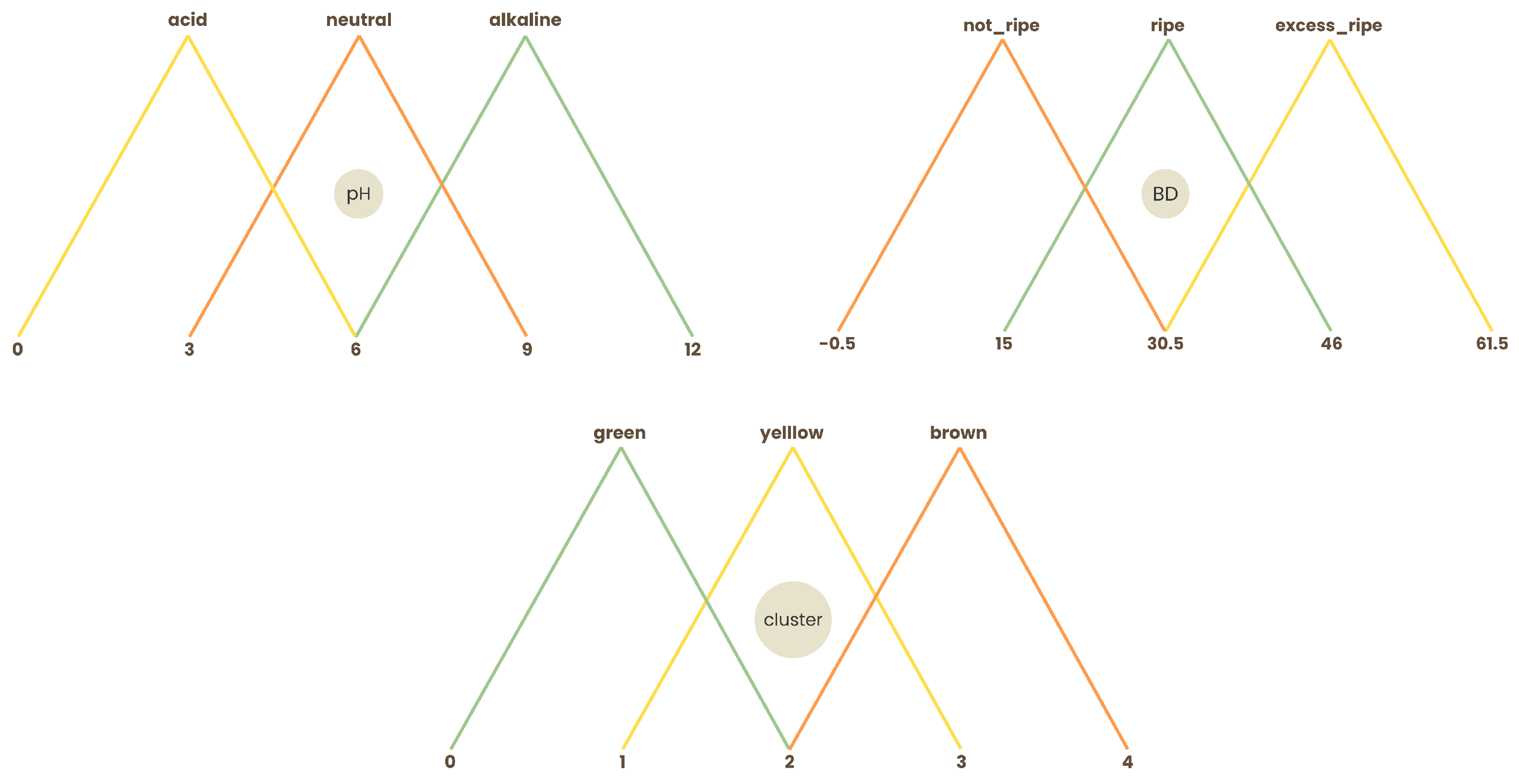
The FIS receives three input variables: BD, soil pH, and a variable derived from leaf colorimetry named Cluster. The ranges for the MFs of each input were established as follows:

• For the BD variable, a two-year historical dataset was used solely as a reference to define its range, based on harvest records provided by Rancho Tajeli. In this dataset, BD values ranged from a minimum of 22 (19 April 2023) to a maximum of 36 (26 September 2024).
• For the pH variable, the default scale was applied based on standard soil acidity and alkalinity measurements.
• For leaf colorimetry, the variable “Cluster” was created based on image processing and grouping, with values ranging from 1 to 3, representing the dominant color cluster in each sample (green, yellow, or brown).

Each of the three input variables was modeled using three triangular MFs. Their parameters are described in

Table 4. Input features.

Variable	Range	Indicator
pH	3–9	acid	neutral	alkaline
		[0 3 6]	[3 6 9]	[6 9 12]
BD	15–46	not_ripe	ripe	excess_ripe
		[−0.5 15 30.5]	[15 30.5 46]	[30.5 46 61.5]
Cluster	1–3	green	yellow	brown
		[0 1 2]	[1 2 3]	[2 3 4]

and shown in Figure 9.

2.3.4. Output Configuration of the FIS

The output of the TSK-type FIS implemented in this study is of constant type, meaning that each FR is associated with a fixed numerical value. In this case, the system generates 27 constant functions, one for each possible combination of input MFs. These output values are derived from assigning three MFs to each of the three input variables, resulting in 3 × 3 × 3 = 27 FRs combinations. Consequently, the model defines 27 constant outputs, each linked to a specific rule.

The output variable is binary, where 0 indicates “Not Harvest” and 1 indicates “Harvest”, enabling a straightforward decision-making process. Output variable parameters are shown in

Table 5. Output features.

Variable	Value	Indicator
Harvest	[0 1]	not_harvest	harvest
		[0]	[1]

.

2.3.5. Fuzzy Rules Structure of the FIS

In an FIS, the FRs are central to translating expert knowledge into model behavior. Each rule establishes a relationship between the input fuzzy sets and the corresponding output, enabling qualitative reasoning within the model. An FR consists of two main components: the antecedent, which defines the condition(s) for activation, and the consequent, which specifies the output response. When multiple conditions are included in the antecedent, Fuzzy Operators (FOs) are used to connect the fuzzy sets involved. The most common operators are AND (intersection), OR (union), and NOT (complement) [44].

A total of 27 FRs were generated in this system, corresponding to all combinations of input MFs. These rules are listed in Appendix A,

Table A1. System fuzzy rules.

FR		Antecedent	FO	Antecedent	FO	Antecedent		Consequent
1		pH is acid		BD is not_ripe		cluster is 1		not_harvest
2		pH is acid		BD is not_ripe		cluster is 2		not_harvest
3		pH is acid		BD is not_ripe		cluster is 3		not_harvest
4		pH is acid		BD is ripe		cluster is 1		not_harvest
5		pH is acid		BD is ripe		cluster is 2		not_harvest
6		pH is acid		BD is ripe		cluster is 3		not_harvest
7		pH is acid		BD is excess_ripe		cluster is 1		not_harvest
8		pH is acid		BD is excess_ripe		cluster is 2		not_harvest
9		pH is acid		BD is excess_ripe		cluster is 3		not_harvest
10		pH is neutral		BD is not_ripe		cluster is 1		not_harvest
11		pH is neutral		BD is not_ripe		cluster is 2	t	not_harvest
12	i	pH is neutral	A	BD is not_ripe	A	cluster is 3		not_harvest
13		pH is neutral		BD is ripe		cluster is 1	h	harvest
14	f	pH is neutral	N	BD is ripe	N	cluster is 2		not_harvest
15		pH is neutral		BD is ripe		cluster is 3	e	not_harvest
16		pH is neutral	D	BD is excess_ripe	D	cluster is 1		not_harvest
17		pH is neutral		BD is excess_ripe		cluster is 2	n	not_harvest
18		pH is neutral		BD is excess_ripe		cluster is 3		not_harvest
19		pH is alkaline		BD is not_ripe		cluster is 1		not_harvest
20		pH is alkaline		BD is not_ripe		cluster is 2		not_harvest
21		pH is alkaline		BD is not_ripe		cluster is 3		not_harvest
22		pH is alkaline		BD is ripe		cluster is 1		not_harvest
23		pH is alkaline		BD is ripe		cluster is 2		not_harvest
24		pH is alkaline		BD is ripe		cluster is 3		not_harvest
25		pH is alkaline		BD is excess_ripe		cluster is 1		not_harvest
26		pH is alkaline		BD is excess_ripe		cluster is 2		not_harvest
27		pH is alkaline		BD is excess_ripe		cluster is 3		not_harvest

.

A summary of the ANFIS parameters used is listed in Appendix B,

Table A2. Summary of ANFIS parameters.

Training Features
Number of inputs	3
Number of outputs	1
Number of training epochs	10
MFs input	3 per input variable
Number of FRs	27
Input FM Parameters
Input 1	MF 1 (acid): trimf-Range: [0 3 6]
	MF 2 (neutral): trimf-Range: [3 6 9]
	MF 3 (alkaline): trimf-Range: [6 9 12]
Input 2	MF 1 (not_ripe): trimf-Range: [−3.5 13 29.5]
	MF 2 (ripe): trimf-Range: [13 29.5 46]
	MF 3 (excess ripe): trimf-Range: [29.5 46 62.5]
Input 3	MF 1 (1): trimf-Range: [0 1 2]
	MF 2 (2): trimf-Range: [1 2 3]
	MF 3 (3): trimf-Range: [2 3 4]
Output Parameters
Output: Constant type	harvest: [1]
	not_harvest: [0]
Neural Network Structure
Number of layers	5
Number of neurons in layer 1 (input MF)	9
Number of neurons in layer 2 (RF)	27
Layer 3	Standardization
Layer 4	Linear functions
Layer 5	Weighted sum

.

2.4. Timely Harvest Prediction Algorithm

Algorithm 1 shows the pseudocode of the proposal to predict the TH in Stevia crops.

Algorithm 1 Timely Harvest Prediction

1: Read data from file  2: Assign inputs and output  3: Initialize:  4:      $n\leftarrow$ number of samples  5:      absolute_residuals ← vector of size n  6:      epoch_number $\leftarrow 10$  7:      mf_type ← ‘trimf’  8: for $i=1$ to n do  9:       Split data into training and testing sets 10:      fismat ← genfis1(training_data, 3, mf_type) 11:      fismat_trained ← anfis(training_data, fismat, epoch_number) 12:      predicted_output ← evalfis(test_input, fismat_trained) 13: end for

In MATLAB, the functions genfis1, anfis, and evalfis are fundamental for working with ANFIS. For this reason, each of these functions is explained in detail below:

2.4.1. GENFIS1 Function

genfis1 (Generate Fuzzy Inference System) is a function that creates an initial TSK-type FIS based on training data. It automatically assigns MFs to the input variables.

Sintax: fismat = genfis1(data, numMFs, MFtype)

• data: A dataset where columns 1 to (m 4 − 1) represent input variables and the m-th column represents the output variable.
• numMFs: Number of Membership Functions per input variable.
• MFtype: Type of Membership Function (e.g., ‘trimf’ for triangular, ‘gaussmf’ for Gaussian).

2.4.2. ANFIS Function

anfis (Adaptive Neuro-Fuzzy Inference System Training) is a function that trains the FIS using a hybrid learning algorithm, combining

-

 Gradient Descent (Backpropagation): Adjusts MF parameters.

-

 Least Squares Estimation (LSE): Tunes linear parameters in the TSK-type FIS.

Sintax: fismat_trained = anfis(training_data, fismat, epoch_number).

• training_data: Same format as genfis1, used for supervised learning.
• fismat: The initial FIS structure (from genfis1).
• epoch_number: Number of training iterations.

2.4.3. EVALFIS Function

evalfis (Evaluate Fuzzy Inference System): This function computes the output of the trained FIS for a given input dataset.

Sintax: predicted_output = evalfis(test_input, fismat_trained).

• test_input: Matrix where each row is an input sample (same number of features as in training).
• fismat_trained: The trained fuzzy system from ANFIS.

2.5. Evaluation Metrics

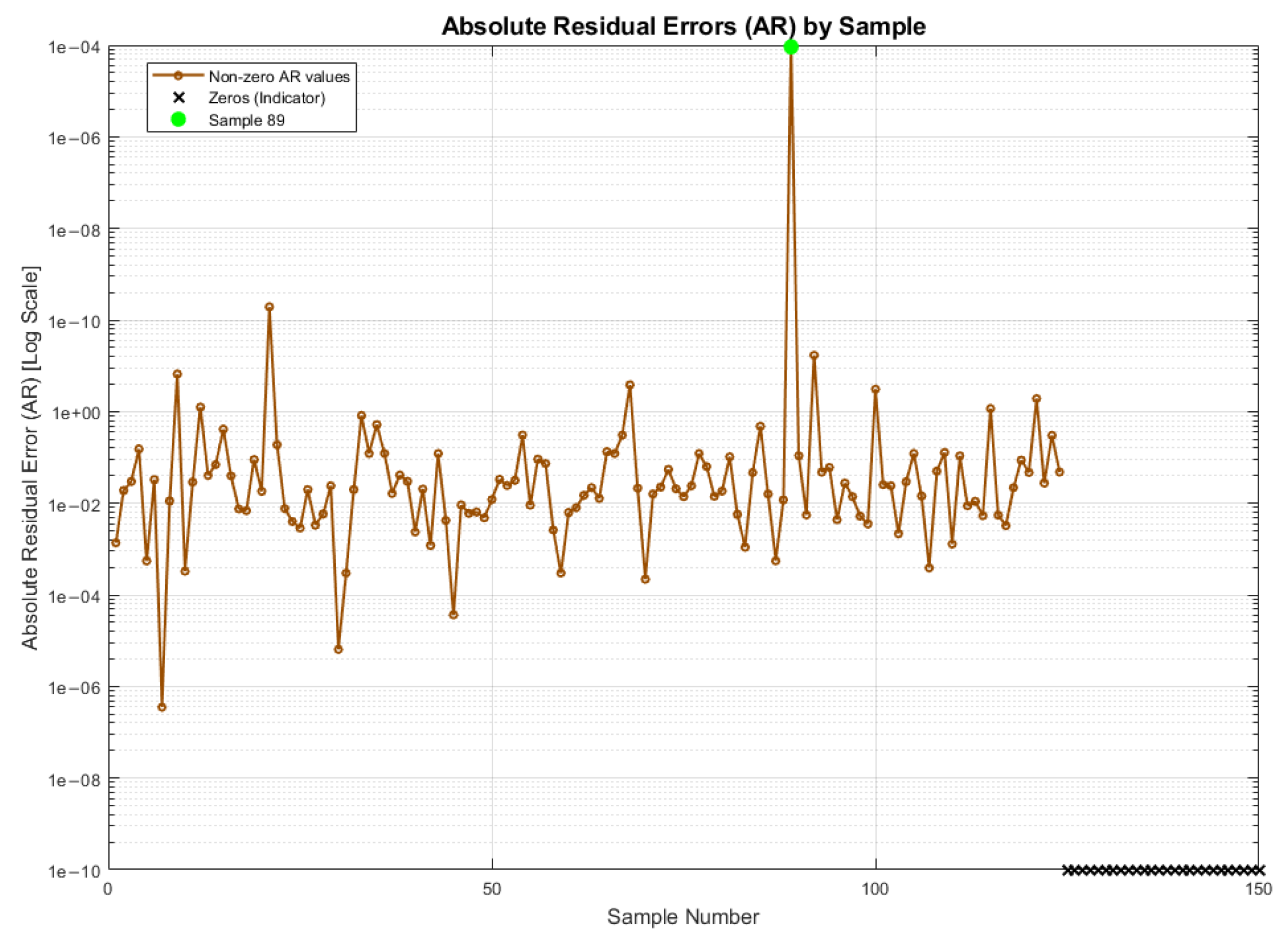
The decision to employ LOOCV in conjunction with the AR metric stems from the recognition that this combination offers a robust and accurate assessment of the ANFIS model within the context of binary outputs. At each iteration of LOOCV, the AR between the predicted and actual output for the test sample is calculated, thereby providing a direct and consistent error metric. Furthermore, by calculating the mean of the AR from all iterations, an overall model error indicator is obtained, enabling the evaluation of the model’s accuracy across the entire dataset.

2.5.1. Absolute Residuals (ARs)

The selection of the AR metric is based on the binary nature of the model output (TH:1, Not TH:0), which implies that the discrepancy between predicted and actual values is discrete. Additionally, this metric provides a straightforward interpretation of the results. The AR metric has been used extensively in several studies, including works such as [45,46,47]. The AR metric is defined by Equation (1).

$$\mathrm{AR}=\left|THActua{l}_{\mathit{i}}-THPredicte{d}_{\mathit{i}}\right|$$

(1)

For each observation i, in which the suitability of the harvest is evaluated, an AR value is calculated. Equation (2) shows the calculation of the mean AR value (MAR) for a set of n observations. This value is obtained by summing the individual AR values and dividing the result by the total number of observations.

$$\mathrm{MAR}={\displaystyle \frac{1}{n}}\sum _{i=1}^n\left|T{H}_{\mathit{i}}\right|$$

(2)

A MAR value approaching zero indicates a heightened degree of accuracy in the prediction technique. This suggests that a low MAR signifies that the model predictions are more aligned with actual values [48].

2.5.2. Leave-One-Out Cross-Validation (LOOCV)

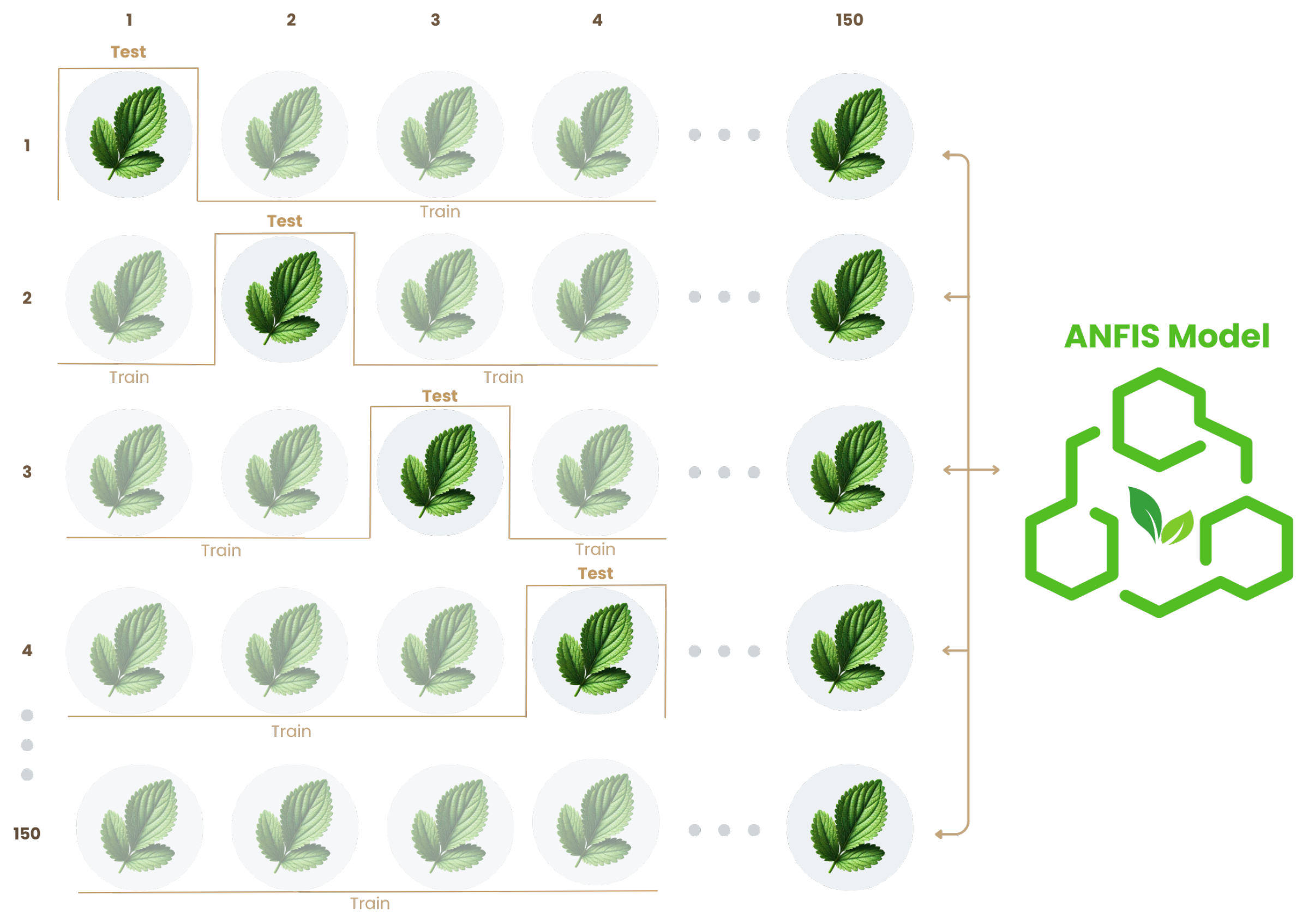
The LOOCV method was employed to assess the performance of the model, as it provides a comprehensive evaluation. This approach ensures that each sample in the dataset is used as a test once, while the remaining samples are used for model training. Consequently, all samples contribute to both the training and validation processes. Studies such as [49,50,51] have implemented the LOOCV technique to partition the data in their models, obtaining accurate results. The operational process of LOOCV is illustrated in Figure 10.

The numbers 1, 2, 3, 4 …150 in the illustration refer to the individual samples in the dataset. In this case, the dataset consists of 150 instances. Each sample is used once as the validation set while the remaining samples are used for training. The numbers visually represent how this procedure is repeated 150 times, one for each data point, ensuring that every instance is evaluated.

2.5.3. Determination Coefficient ($r^2$)

In a simple linear regression analysis, the coefficient of determination, denoted as $r^2$, quantifies the proportion of the dependent variable’s total variance that is accounted for by the independent variable. Specifically, $r^2$ represents the ratio of the model’s explained variance (SSM) to the total variance of the dependent variable (SST) [52], as expressed by Equation (3):

$$r^2={\displaystyle \frac{SSM}{SST}}={\displaystyle \frac{\sum {({\widehat{y}}_i-\overline{y})}^2}{\sum {(y_i-\overline{y})}^2}}$$

(3)

A predictive model is considered acceptable when the $r^2\ge 0.5$ [53]. The $r^2$ metric has been extensively utilized for the evaluation of studies as evidenced by the literature [54,55,56].

2.6. App Development

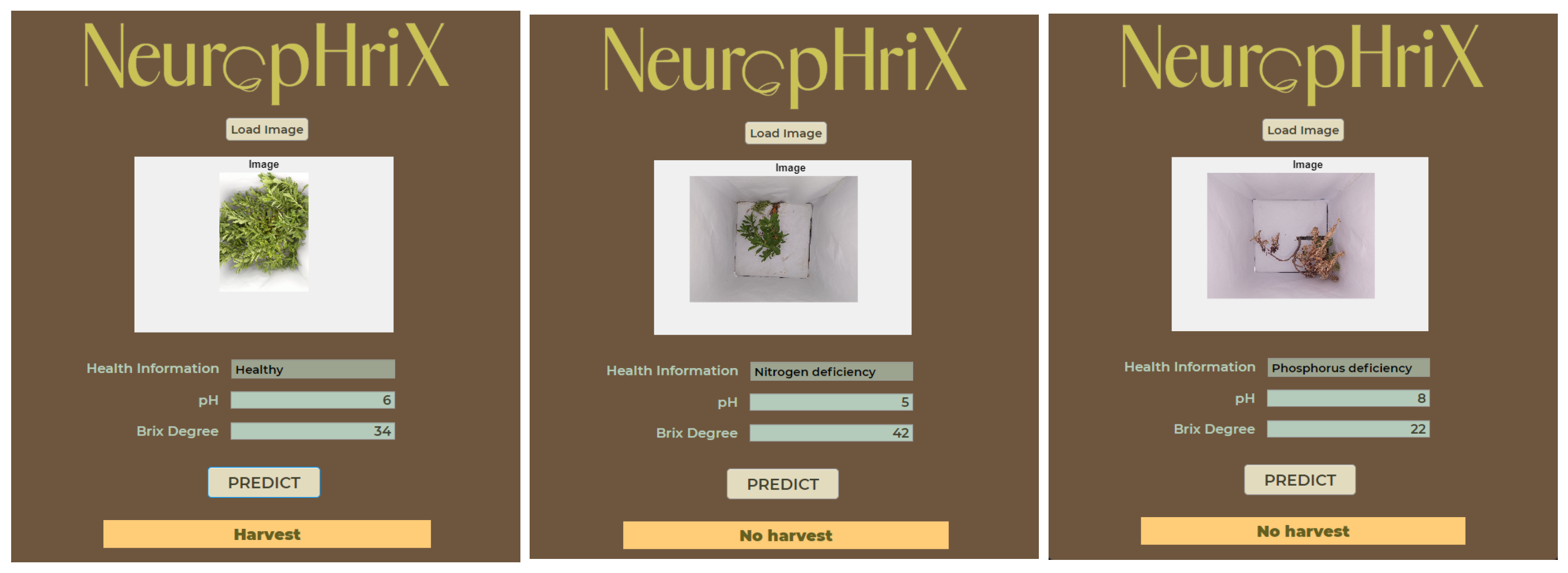
An application was designed using the App Designer Toolbox within the MATLAB environment. The objective of the design was to provide the end user with an intuitive and accessible tool to determine if the crop can be harvested.

In the interface, the user can load an image of the Stevia crop using the “Load Image” button. The image is automatically processed and, depending on the cluster assigned during this processing, a brief description of the plant status is displayed. Subsequently, the user is prompted to enter the pH and BD values. Finally, by tapping the “Predict” button, the application shows the result, indicating whether or not the plant is suitable for harvesting. The performance of the application is illustrated in Figure 11, through a series of tests.

3. Results

3.1. Model Evaluation with Original Data

The evaluation of the ANFIS model was developed through the metrics mentioned in Section 2.6. The evaluation process involves the partitioning of the dataset, whereby in each iteration of LOOCV, a simple sample (i-th sample) is designated as a test sample, while the remaining samples (n − 1) are utilized for training. Subsequent to the training of the model, a prediction is made for the sample that was excluded, and this is then compared when all data have been processed. In this study, the process is repeated 150 times.

The errors obtained after submitting the model to evaluation are visualized in Figure 12. This graph shows that sample 89 exhibits the highest error, with a value of 0.09597, while samples 125 to 150 demonstrate the lowest errors.

Following the execution of the evaluation, a MAR of 0.00064305 was obtained. This finding indicates that the prediction accuracy of the ANFIS model is optimal. On the other hand, in the evaluation of the model with the $r^2$ metric, the LOOCV technique was also used, obtaining a value of 0.99965. This outcome signifies a highly precise fit, thereby classifying the model as both acceptable and robust in terms of predictive capacity.

3.2. Model Evaluation with Synthetic Data

3.2.1. Synthetic Data Generation

The dataset size used in this study was constrained by the availability of plants at the time of data acquisition. Since a dataset comprising 150 samples is relatively small for the implementation of machine learning techniques, synthetic data generation was employed to enhance the model’s representativeness. Synthetic data were generated by adding Gaussian noise, which is a random variation following a normal distribution. In this context, the generated values are distributed around the mean, preserving the statistical structure of the original data to evaluate the robustness of the model.

3.2.2. Performance with Synthetic Data

Two synthetic datasets were generated, one comprising 1000 samples and the other 10,000 samples. Both datasets were generated while preserving the statistical characteristics and trend of the original dataset, ensuring consistency in variable distribution.

Subsequently, the system was evaluated using both datasets, yielding the following results (

Table 6. Tests with synthetic data.

Dataset	Computational Cost	MAR	${\mathit{r}}^2$
150	1 min, 45 s	0.00057944	0.99965062
1000	8 min, 11 s	0.00000201	0.99999999
10,000	3 h, 59 min, 19 s	0.00000016	0.99999999

).

A statistically significant difference is observed in terms of computational cost, favoring the proposed model. However, in terms of the MAR and $r^2$ values, the statistical difference is not significant.

4. Discussion

A comprehensive literature review conducted by the authors revealed that no previous studies specifically address TH prediction in agricultural systems, nor in Stevia crops. While research in agriculture and intelligent systems has explored areas such as pest forecasting, greenhouse control, fruit grading, and irrigation optimization, no existing work has proposed an NFS for TH assessment. This study introduces a novel approach by integrating soil pH, BD, and leaf colorimetry as key agronomic indicators, leveraging adaptive fuzzy inference to facilitate an objective, data-driven harvest decision-making process. The following sections provide a broader perspective on existing methodologies, positioning the proposed model in context and exploring opportunities for future development.

4.1. Existing Approaches and Their Scope

Predicting TH in crops is a complex task due to the multiple environmental and physiological factors influencing crop maturity. Traditional methods rely on visual inspection or predefined harvest schedules, which can lead to variability in decision-making and potential yield losses. In this study, an NFS based on the ANFIS architecture was proposed to predict TH in Stevia crops, integrating soil pH, BD, and leaf colorimetry as input variables.

Several studies have successfully implemented ANFIS-based models in agricultural applications, demonstrating their effectiveness in handling nonlinear relationships and integrating expert knowledge with data-driven learning. For instance, Hashem et al. [57] used ANFIS for assessments of oilseed production, benefit/cost ratio in agricultural systems, achieving an $r^2$ of 0.87. Also, Lotfali et al. [58] compared ANFIS and ANNs for energy flow analysis in oilseed farms, reporting a higher $r^2$ value of 0.94 with ANFIS, highlighting its superior predictive capability.

In climate and drought prediction, Hobart et al. [59] employed Wavelet-ANFIS to forecast the Temperature and Vegetation Dryness Index (TVDI) in mango orchards, obtaining an $r^2$ of 0.95, demonstrating ANFIS’s adaptability to environmental modeling. Moreover, Durmuş et al. [60] assessed the potential reuse of treated wastewater in agriculture, utilizing ANNs, ANFIS, and Fuzzy Logic-Mamdani (FLM), with $r^2$ values ranging from 0.74 to 0.96, reinforcing the relevance of hybrid machine learning techniques in agricultural optimization.

Despite these advancements, some studies report lower $r^2$ values when using ANFIS in soil analysis applications. Han et al. [61] applied multiple linear regression (MLR), partial least squares regression (PLSR), random forest regression (RFR), and ANFIS to estimate heavy metal content in agricultural soil, achieving $r^2$ values between 0.653 and 0.713, which may be attributed to the complexity of soil composition and the influence of external environmental factors.

4.2. How the Proposed Approach Stands Out

The ANFIS-based model developed in this study achieved an $r^2$ of 0.99, outperforming the majority of previously reported models. This suggests that the integration of pH, BD, and leaf colorimetry provides strong predictive power for TH assessment in Stevia crops. Despite the fact that the approaches reviewed in the previous section exhibit acceptable $r^2$ values, none surpass the predictive accuracy of the model proposed in this study.

Table 7. Comparative table of other proposed approaches using ANFIS and the one proposed in this study.

Reference	Study Object	AI Technique Used	${\mathit{r}}^2$ Obtained
Hashem et al. [57]	Benefit/cost ratio in agricultural systems	ANFIS	0.87
Lotfali et al. [58]	Energy flow analysis in oilseed farms	ANFIS, ANN	0.94
Hobart et al. [59]	Temperature and Vegetation Dryness Index (TVDI) prediction	Wavelet-ANFIS	0.95
Durmuş et al. [60]	Potential of treated wastewater	ANNs, ANFIS, and Fuzzy Logic-Mamdani (FLM)	0.74–0.96
Han et al. [61]	Estimation of heavy metal (Loid)	Multiple Linear Regression (MLR), Partial Least Squares Eegression (PLSR), Random Forest Regression (RFR), and ANFIS	0.653–0.713
Proposed approach	Prediction of TH in Stevia crops	ANFIS	0.99

presents a comparative analysis, highlighting the differences between the previously discussed methodologies and the proposed ANFIS-based system.

Additionally, unlike some machine learning approaches that require large datasets, ANFIS demonstrated reliable performance even with a limited dataset of 150 samples, benefiting from its adaptive rule-based inference. Furthermore, to assess the scalability and robustness of the proposed model, it was tested using synthetic datasets containing 1000 and 10,000 samples. As observed in Table 6, increasing the dataset size led to a notable increase in computational cost compared to the baseline dataset of 150 samples. While it might be expected that a larger dataset would improve model accuracy, the AR and $r^2$ values showed only marginal differences across dataset sizes. This suggests that the model does not exhibit a clear trend of higher precision with increasing data volume.

However, the impact on computational efficiency was significant. The training time for the dataset of 10,000 samples was approximately 3 h and 57 min longer than that for the 150-sample dataset, indicating a substantial increase in processing requirements. This result highlights a key consideration for real-world applications: while data augmentation can be useful, it may not always translate into a proportional increase in predictive accuracy and may lead to diminishing returns in terms of model performance. Therefore, optimizing dataset size and computational resources should be carefully balanced when scaling up the proposed ANFIS model.

Another critical aspect of predictive agricultural models is their adaptability to different environmental conditions. Unlike traditional models that require complete retraining when new variables or crop types are introduced, ANFIS allows modifications to FRs and MFs without requiring a full retraining cycle, making it more flexible for real-world agricultural applications. This adaptability was also highlighted in Hobart et al. [59], who demonstrated ANFIS’s capability in adapting to climate variations in drought monitoring.

4.3. Future Work

Several research directions could further enhance the proposed system:

• Expansion of Input Variables: Incorporating additional parameters such as soil electrical conductivity, microbial activity, or leaf chlorophyll content may improve prediction accuracy by integrating more physiological indicators of crop maturity.
• Comparative Analysis with Alternative Models: Evaluating the ANFIS model against other techniques, such as TSK fuzzy models or hybrid deep learning approaches, could provide insights into its relative performance and potential optimizations.
• Refinement of Clustering Techniques: Exploring alternative unsupervised learning algorithms, such as Gaussian Mixture Models (GMM) or Density-Based Spatial Clustering (DBSCAN), may enhance the segmentation and classification of leaf color data.
• Large-Scale Deployment via Cloud Integration: Implementing the system on web-based platforms with cloud database access would facilitate real-time data collection, enabling continuous crop monitoring and decision support for farmers.
• Field Validation and Adaptability Studies: Conducting on-site testing under different environmental and agronomic conditions would allow for the model’s adaptation to diverse farming scenarios, improving its generalization capabilities.

By addressing these aspects, the proposed system can evolve into a scalable and adaptable decision-support tool for precision agriculture, enhancing crop management strategies and increasing harvest efficiency in Stevia production.

5. Conclusions

The objectives established in this study were successfully achieved. A predictive system based on ANFIS was developed to classify Stevia crops as ready for harvest (TH = 1) or not (TH = 0) using soil pH, BD, and leaf colorimetry as key agronomic indicators. The model’s feature extraction process effectively converted leaf color into numerical values, ensuring compatibility with the ANFIS inference mechanism. The system’s accuracy and generalization performance were rigorously evaluated using AR and LOOCV, confirming its reliability. Additionally, a comparative analysis with synthetic datasets (1000 and 10,000 samples) demonstrated that while scalability increased computational cost, it did not significantly alter predictive accuracy. These findings validate the effectiveness, adaptability, and robustness of the proposed approach, positioning it as a valuable tool for PA.

The model provides an automated and quantitative approach to assessing crop maturity, reducing subjectivity in harvest decision-making. It is important to highlight that, based on the literature review conducted, no prior studies specifically address TH prediction in agricultural systems or Stevia crops, making this approach a novel contribution to PA.

An experimental evaluation using 150 Stevia plants demonstrated that the model yielded highly accurate predictions, with an $r^2$ of 0.99965, surpassing similar ANFIS-based applications in agricultural modeling. The AR metric also confirmed the low deviation between predicted and actual values, reinforcing the model’s robustness and reliability. To further assess scalability and computational efficiency, the model was tested with synthetic datasets of 1000 and 10,000 samples, revealing that, although the use of larger datasets resulted in a substantial increase in computational cost, the observed differences in predictive accuracy were statistically insignificant. This suggests that data volume did not yield a significant enhancement in model performance, despite the added computational burden.

The results of this study validate the effectiveness of ANFIS for crop maturity prediction, highlighting its flexibility, adaptability, and ability to generalize with limited data. Unlike purely data-driven models, the proposed system combines expert knowledge with machine learning, ensuring reliable predictions even with small datasets.

This development has the potential to be applied to other crops by adapting specific parameters, aligning with strategic agricultural projects and supporting high-impact farming activities at various scales.