Analyzing the Risk of Short-Term Losses in Free-Range Egg Production Using Commercial Data

Abstract

Free-range egg production plays a key role in the global food system, and current market trends suggest that consumer demand for free-range eggs will continue to rise. Free-range egg production is susceptible to a wide range of factors, including climatic conditions, management practices, and disease presence. These factors can cause variability in the laying rate of a flock over time, leading to fluctuations in egg production. The main purpose of this study was to investigate the risk of short-term free-range egg production losses using data derived from a combination of sensing technologies and management activities. Production and environmental data were collected from a commercial farm comprising seven flocks of laying hens. The variables studied included laying rate, feed intake, water intake, solar radiation, humidity, precipitation, and indoor/outdoor temperature. These were processed into a set of aggregate features calculated across a 14-day moving window. Generalized estimating equations were used to analyze the association between the derived production and environmental features and the probability of a short-term drop in egg production, expressed through deviations in the laying rate on the day immediately following the data window. Odds ratios were used to express the relative risk of a production drop by comparing the features for window periods where production drops occur to the window periods where production drops did not occur. The results demonstrated that a range of data features based on the laying rate, feed intake, water intake, and indoor/outdoor temperatures all had significant associations with the odds of a production drop. Key findings from the study show that an increase in feed intake and laying rate measured across the 14-day data window were correlated with a lower risk of a sudden drop in egg production. Conversely, a low mean indoor temperature (x < 16.1 °C group), measured through environmental sensing data, was correlated with a higher risk of a sudden drop in egg production. This study quantifies the link between data features derived from production and environmental monitoring and egg production issues, thereby providing useful insights on the most important data items captured through day-to-day monitoring, which can be used for proactive management. Further research should be carried out to investigate how technologies such as machine learning and analytics platforms can be applied for the task of forecasting production interruptions using the data features explored in this study.

1. Introduction

The global production of eggs has increased in recent years and eggs are essential for meeting the nutritional demands of many households. Free-range eggs have become popular due to the rise in consumer preference for ethically sourced eggs, prompting an increase in production [1,2]. The Australian egg industry is observing a dramatic increase in free-range egg sales values accounting for 61.9%, followed by caged eggs at 15.7% and barn-laid eggs at 18.4% and specialty eggs 4%, within the 2023–2024 fiscal year [3]. While the production of free-range eggs has increased over time, free-range systems face numerous challenges that can result in sudden fluctuations of egg production, thereby impacting farm profitability. Therefore, there is a need to identify the factors that are responsible for these sudden egg production losses.

Many of the challenges experienced by free-range egg production are related to environmental factors including fluctuating weather conditions, predators, and diseases [4,5,6]. The physical state of hens can be influenced by weather parameters such as temperature, relative humidity, rainfall, and sunlight [7]. Heat stress, resulting from higher ambient temperatures, can lead to metabolic alkalosis and reduced feed intake thereby causing thinner eggshells, reduced egg size, and overall lower egg production [8,9]. Furthermore, decreased egg performance and high mortality rates among free-range hens can be caused by smothering, stress, and poor health management practices [10]. While data that are collected through the day-to-day operations of commercial free-range egg farms can measure and characterize many of these adverse production conditions, their utilization in forecasting tools and risk assessment is currently not common.

The hardware and housing systems employed in modern egg production typically incorporate a range of sensing technologies that provide real-time monitoring for different aspects of production. Environmental conditions such as temperature, humidity, air quality, and ventilation generally are monitored to ensure compliance with animal standards [11] using commercial sensor packages [12] that offer direct connectivity to analytical systems. Other aspects of production including the feed intake and water intake are monitored indirectly by weighing feed silos and using flow-rate sensors across water lines to estimate the average per-hen consumption. The collection of eggs can be automated with belt systems to transfer eggs from nesting areas, allowing them to be automatically counted and weighted in high volumes [13,14]. These sensors can be incorporated directly into aviary systems and provide an effective indication of production efficiency. The data produced by the combination of the different technologies have the potential to identify patterns and trends, forecast production issues, and allow better-informed decision-making.

Previous studies have demonstrated that historical production/environmental data can be employed to forecast potential production issues and predict the laying rate using machine-learning models [15,16,17]. The research presented in [15] investigated the use of a Support Vector Machine (SVM) model to detect problems in egg production. The study used production data (and the derived machine learning features) that were focused primarily on patterns in the historical laying rate. It was reported that the SVM model exhibited high accuracy (approximately 0.985) in predicting egg production fluctuations one day in advance. A Random Forest (RF) model was used by [16] to predict daily egg production fluctuations using similar data features to those under study in [15]. It was found that the model performed well, achieving R² values of 0.94 and 0.78 and root-mean-squared error (RMSE) values of 0.176% and 0.368%. The work presented in [17] introduced a fuzzy predictive model for forecasting the future laying rate. Their model demonstrated a high degree of accuracy (approaching 100%) with an approximate mean magnitude relative error (MMRE) of 0.11744. Overall, the previous work in this area has focused on forecasting egg production and its fluctuations using machine learning approaches. Within this body of work, there is no clear knowledge of the risk factors associated with the individual predictors used. The current study addressed this knowledge gap by examining the link between fluctuations (i.e., sudden drops) in egg production and the variables (and their derived features) measured through day-to-day monitoring of egg production.

In this study, we have investigated the associations between short-term egg production losses and features derived from data collected through systems incorporated into commercial egg production along with weather data collected from public monitoring services. We aimed to identify the most important factors, measurable through day-to-day technology, and investigate the nature of their relationship to short-term egg production losses in free-range hens. The outcomes from this study will allow producers to prioritize the integration of specific data items into their decision-making processes (or analytics systems) and can be used to inform the future development of monitoring and machine learning approaches to forecast production issues using diverse, multidimensional datasets. This study contributes to the field of data-driven decision-making in agriculture by demonstrating the potential of commercial production and environmental data in predicting short-term egg production losses. The remainder of this manuscript describes the collection of the underlying dataset (Section 2.1), defines the aggregate data features calculated for the study (Section 2.2), outlines the process for identifying sudden drops in the laying rate (Section 2.3), and describes the statistical modeling workflow (Section 2.4 and Section 2.5) applied to analyze the risks of sudden laying rate drops in response to the data features. The results for each variable measured are presented in Section 3 along with a detailed discussion with concluding remarks in Section 4 and Section 5 that link the results presented to the wider body work in this area.

2. Materials and Methods

2.1. Dataset

A raw dataset was collected from a commercial laying farm, including seven flocks of Lohmann Brown and Hy-Line Brown hybrids. Each flock was housed in two three-tier aviary systems using chain-feeding and integrated watering systems (Natura Step, Big Dutchman, Vechta, Germany) with access to an outdoor range provided via pop-hole openings. The collected dataset included variables consisting of the laying rate, hen age (in days), mortality rate, feed intake, and water intake. The laying rate was calculated using the total number of eggs collected daily (counted via an integrated egg counter). Daily mortality was manually tracked by workers and subtracted from the flock populations for accurate calculation of laying and mortality rates. Feed intake was measured daily using a silo weighing system integrated into the chain-feeding system and water intake was measured using a flow monitoring system integrated into the aviary system. These measures were expressed as grams of feed per-hen per-day, and milliliters of water per-hen per-day, respectively. The production dataset was extended with climatic variables consisting of the indoor and outdoor minimum and maximum temperatures, relative outdoor humidity at 9 a.m. and 3 p.m., solar radiation, and precipitation. The indoor minimum and maximum temperatures (dry-bulb temperatures) were measured using environmental sensing packages installed in each shed. The dataset was cleaned to remove any invalid production data, and any missing values were replaced with mean values calculated from simple rolling interpolation. The resulting dataset contained 7 flocks, comprising 2772 individual days’ worth of the data.

Table 1. Raw data items are taken from the farm where the production data and weather data modeled for the location.

Parameter	Unit	Summary of Justification	Reference
Laying rate	%	Indicates productivity	[15]
Mortality rate	%	Indicates disease incidence or management problems	[18,19]
Feed intake/hen/day	g	Influences the nutrient intake and egg production	[20,21]
Water intake/hen/day	mL	Needed for metabolic processes and egg production	[22]
Indoor minimum/maximum temperature	°C	Affects egg production and hen health	[23,24]
Relative humidity 9 a.m./3 p.m.	%	Influences hen performance	[7,25]
Outdoor minimum/maximum temperature	°C	Affects egg production	[26]
Precipitation	mm/day	Influences egg production and weight	[27]
Solar radiation	MJ/m2/day	Influences egg production and range use	[28,29]

summarizes the production data collected for each day and environmental data collected using interpolated data from the Bureau of Meteorology modeled for the farm’s location. Table 1 also summarizes the justifications for including each variable along with the reference for previous studies that support the justification. More generally, the combined raw dataset captures both key production variables, such as those adopted in [15,16], and the environmental indicators under study in [17].

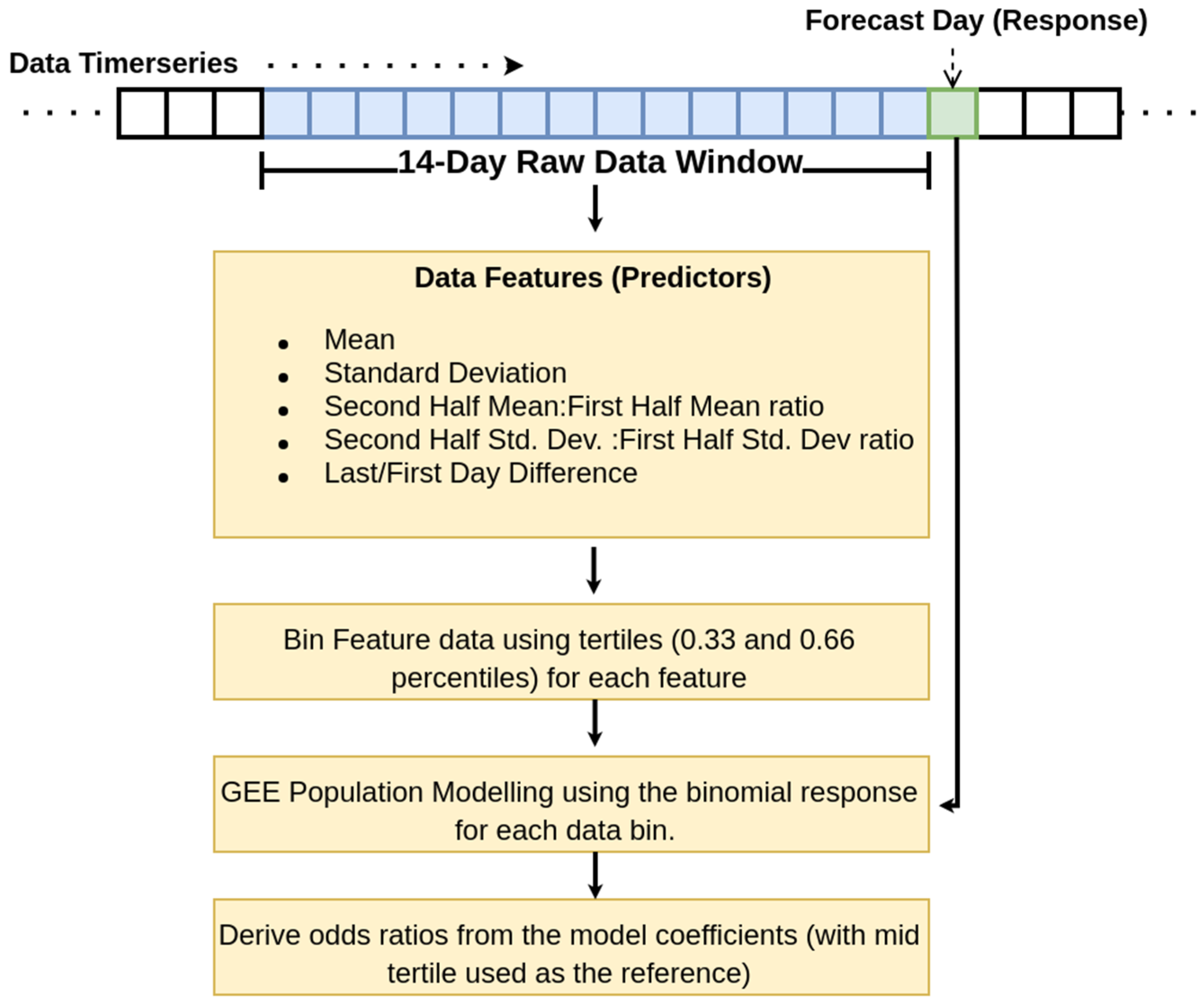
2.2. Feature Dataset

The raw data underwent pre-processing to transform it into time-series data suitable for generalized modeling. Modeling based on these data features involved extracting the relevant characteristics through summary values of the input data. Feature extraction involves identifying and selecting the most informative aspects of the data that are relevant to the task at hand. These features served as the input for the modeling process and helped prevent overfitting. This method was particularly useful when dealing with high-dimensional or complex data where raw information may have contained noise or irrelevant details. By focusing on key features, models can learn generalized patterns and relationships more effectively, leading to improved efficiency and performance. This approach was demonstrated in the studies by [15,16,17] where data features calculated from a raw time series were used to train machine learning models. The feature extraction approach adopted for this study followed the same scheme presented in [15], where aggregate values were calculated across the data for days that fall within a sliding window that was moved day-by-day across the timer series data. This approach aimed to capture the generalized trend of the raw data while limiting the effect of outliers that may cause a model to overfit the underlying data. The study presented in [15] tested window lengths of 7, 14, 21, and 28 days, with the 14-day window providing the highest forecasting performance. As such, the work presented here builds on the previous study by using the 14-day sliding window to calculate a set of data features for each raw data item. The features calculated across the sliding window consisted of:

• Mean;
• Standard deviation;
• The ratio of the mean calculated across the second half of the window to the mean calculated across the first half of the window is denoted as SH mean/FH mean ratio. This feature provided a reliable indication of the trend of the raw feature;
• The ratio of the standard deviation calculated across the second half of the window to the standard deviation across the first half of the window is denoted as the SH Std. Dev/FH Std. Dev. This feature provided an indication of the variation in data features across the window;
• The difference between the first and last day of the 14-day window is denoted as the last day–first day difference. This provides a more sensitive indication of production trends over time, compared to the SH mean/FH mean ratio.

The result of this process was a dataset consisting of the 5 aforementioned data features calculated for each raw data item, across the 14-day sliding window applied across each day for all raw data. The data features adopted for this analysis were analogous to those used in previous machine learning studies and will provide a valuable understanding of the relevant associations with production outcomes.

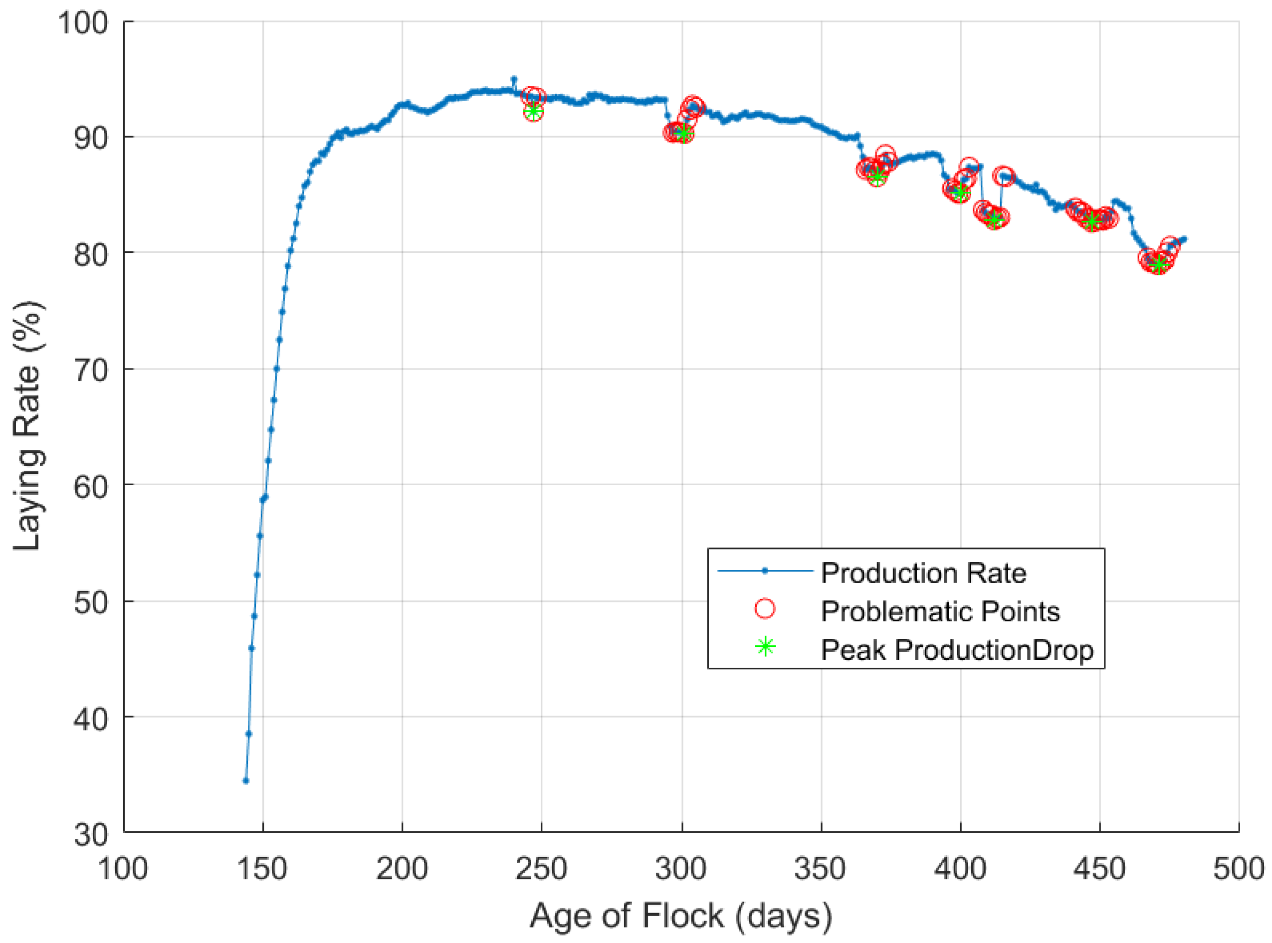
2.3. Detection of Short-Term Production Losses

Short-term reductions in the laying rate for a flock were represented using a binary parameter that specifically targets the production days that form part of a problematic fluctuation in the laying rate. This parameter simply flags a production day as problematic (1) or normal (0), resulting in a simple binary classification scenario. This is an extension of the approach adopted in [15], where, instead of using a manual coding process, we defined a more rigid parameter-based definition to identify potentially problematic days. To construct this parameter, sudden reductions in the egg production rate curves were automatically detected by analyzing the laying rate time-series data for each flock included in the analysis. A rolling window approach was used that identified local minimums in the data by comparing each data point to the average laying rate from the proceeding 7 days. The fluctuations in the curve, which defined sudden reductions in egg production, were then included in the final set based upon two parameters: prominence and duration:

• The prominence of a drop measured how much the peak stood out due to its intrinsic height and its location relative to the surrounding data points. The prominence was measured by taking the distance halfway between the mean of all values in the window and the lowest point in the window. The value for this parameter was set to 2.5 based on numerical inspection of the resulting flagged data points within each production curve using a prominence range of [0.5–3.0]. Through the numerical inspection, it was identified that values for the prominence of <2.5 resulted in the detection of relatively minor fluctuations in the laying rate that were not consistent with fluctuations in the laying resulting from production issues. Conversely, prominence values > 2.5 failed to detect many of the major fluctuations that were consistent with production issues. The prominence value of 2.5 was applied across the production curves of all flocks under study to ensure a consistent detection of production drops.
• The duration was defined by the minimum number of data points that comprised the sudden drop in the laying rate. The value was set to 3 days—where a reduction in egg production with a duration shorter than this was excluded to account for the common day-to-day variations in daily egg collection procedures. This threshold prevents variations such as single-day fluctuations that would typically indicate a collection issue (counting error, equipment failures, etc.) from being detected as a production fluctuation.

The application of this approach identified 235 problematic production days across the dataset resulting in a rate of 8.5 problematic days per 100 days of production. These problematic production days identified within each curve using this process were manually reviewed to ensure that the segments reflected genuine sudden short-term production losses rather than expected production trends (e.g., the relatively slow reduction in the laying rate expected at the end of a flock’s productive life).

2.4. Generalized Estimating Equations

From the feature sets calculated, the 14-day dataset was selected and data for each feature was classified into 3 groups (“bins”) based on tertiles across the distribution of values within each feature. This resulted in the bottom third, middle third, and top third of the data falling into separate equally sized bins. Creating the groupings in a manner allows for the relative frequency of the observations in the data to drive the analysis and ensure that there are enough representative data points to make meaningful inferences. The 14-day dataset was selected for this initial study based on the performance results presented in previous studies [15,16]. A single univariate model for each bin was produced using the generalized estimating equation (GEE) approach [30]. GEEs are an extension of generalized linear models and provide a method for modeling longitudinal or clustered data. They follow the general form given by (Equation (1)):

$$g\left(\mu \right)={\mathsf{\beta }}_0+{\mathsf{\beta }}_1\left(x\right),$$

(1)

where $g\left(\mu \right)$ is the link function, $\mu$ is the expected value of the response variable, ${\mathsf{\beta }}_0$ and ${\mathsf{\beta }}_1$ are the regression coefficients that are to be fitted, and $x$ is the predictor variable.

This model is usually used with non-normal data such as binary or count data. The GEE modeling approach was chosen as it provides a robust way to model population-averaged effects (in this case the probability of a production drop) across a dataset containing repeated, and possibly correlated, measures. Generalized estimating equations were used to model the relationship between individual summary variables (i.e., the predictor value $x$) and the probability of a laying production drop for the day following the data window (i.e., the existence of one of the problematic production points demonstrated in Figure 1). The GEE models developed in this study utilized Bernoulli distribution to model the binary response variable (production drop or no drop on the day following the production window) coupled with the logit link function. A First-Order Autoregressive (AR1) correlation structure was adopted with the flock specified as the subject variable and the hen age as the single within-subject variable, representing the chronological relationship between repeated measures. This approach allowed the GEE models to correctly account for the changes exhibited by each flock as management practices and climatic conditions change across the lifecycle of the flock. The GEE approach has been applied across a range of areas for the analysis of longitudinal data (e.g., time-series data) because it has the advantage of being less sensitive to the variance structure specification compared to generalized linear mixed models [31,32]. The GEE models were implemented using the GEEQBOX toolkit [33] running within MATLAB 2019a [34].

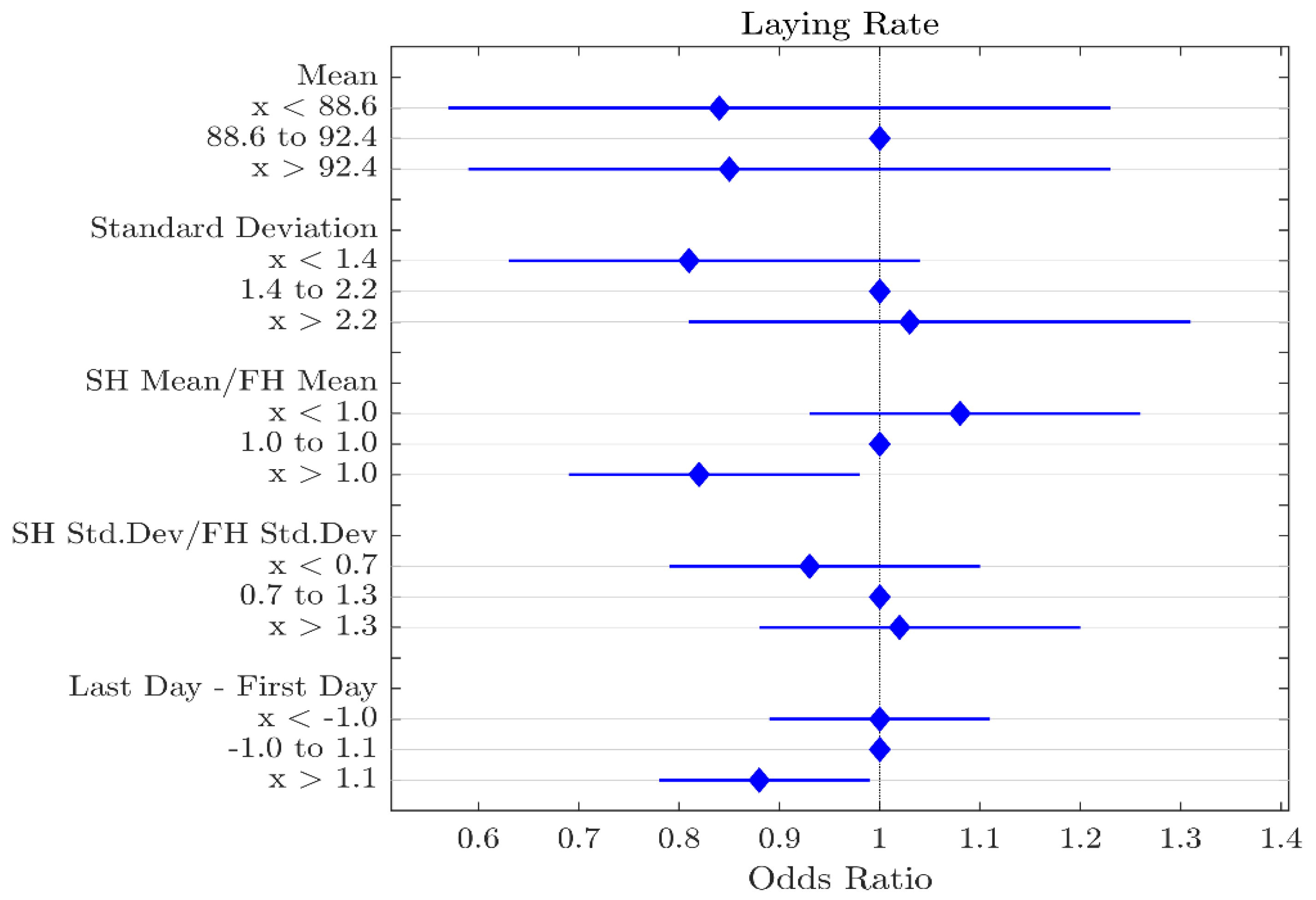
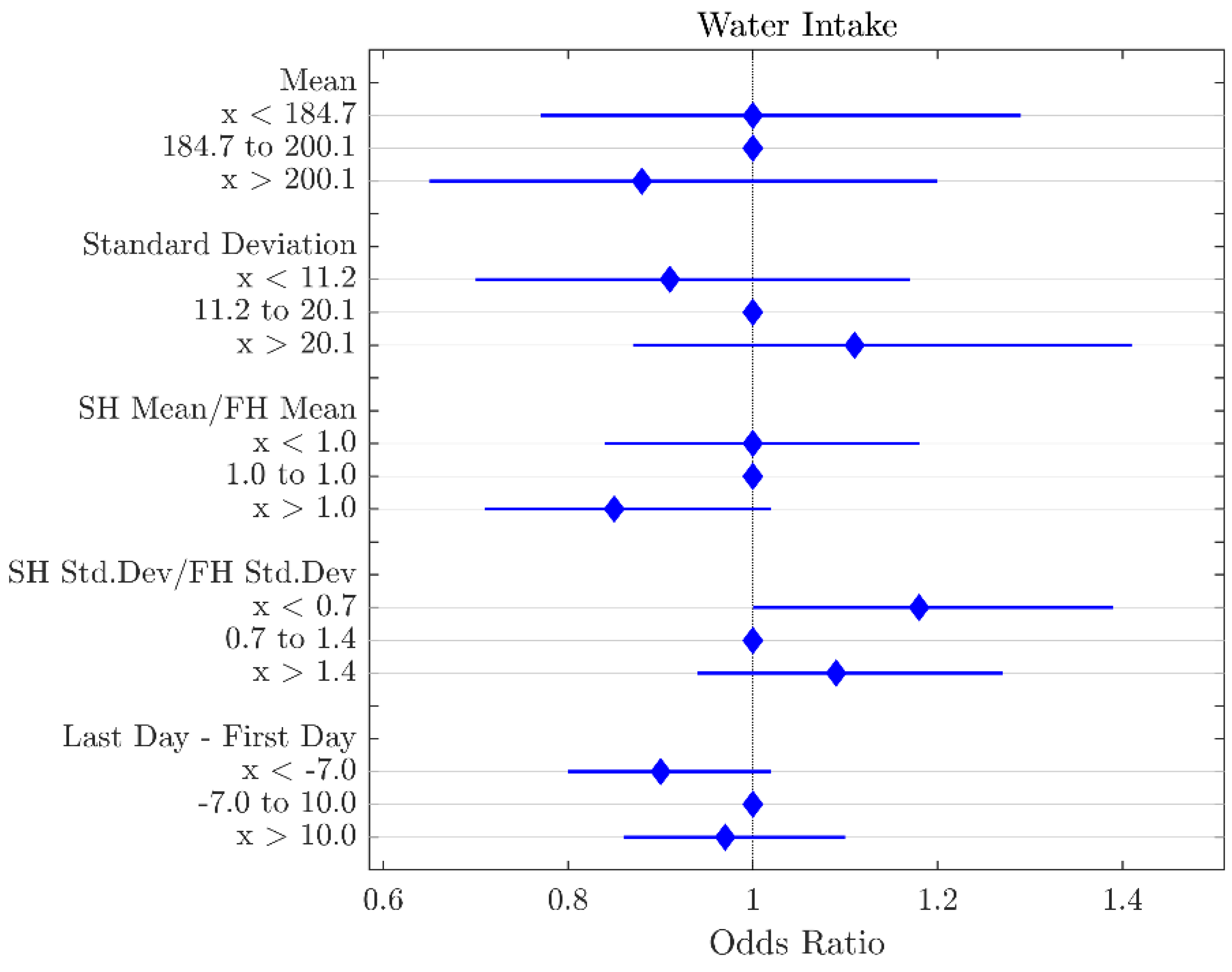
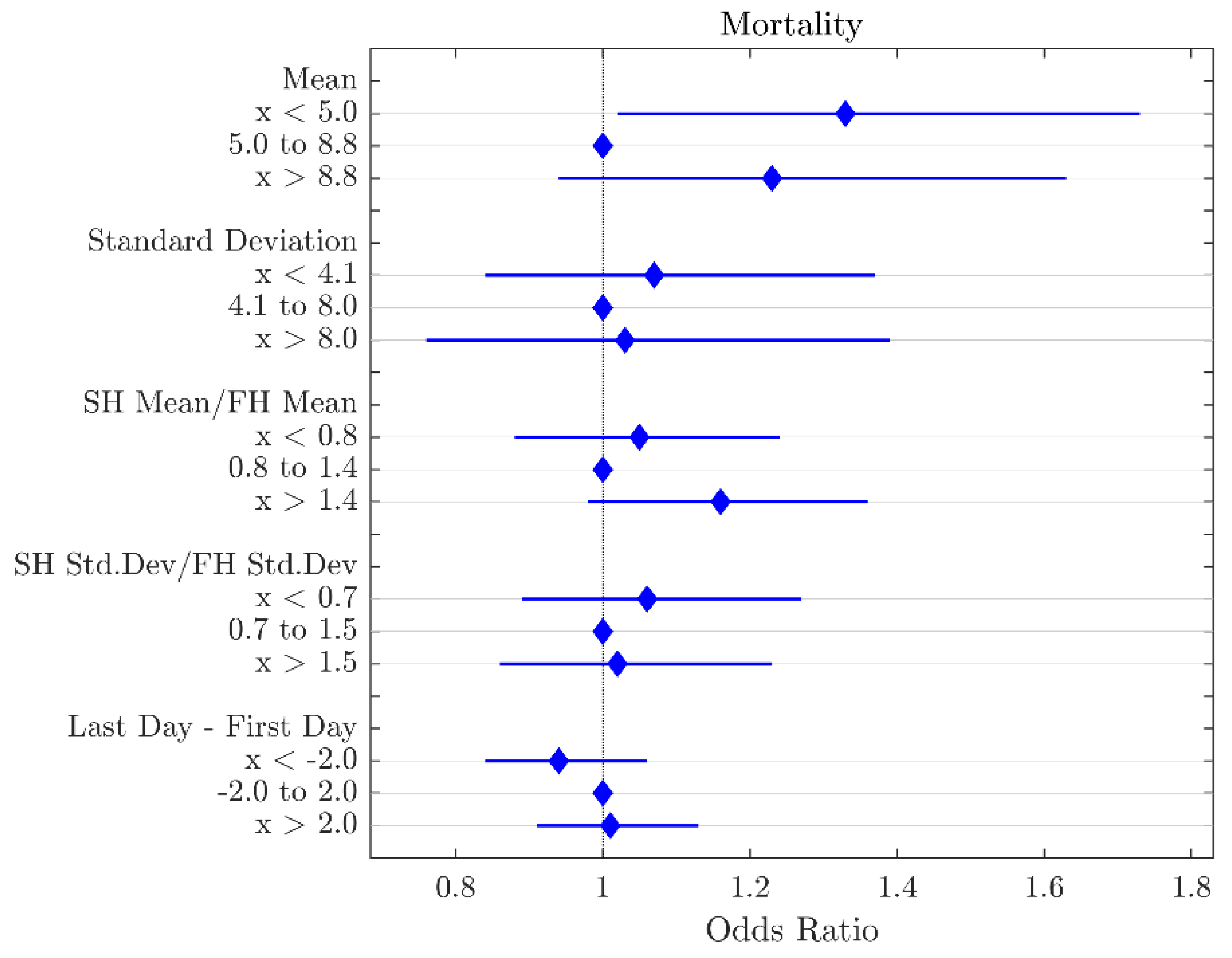
2.5. Odds Ratio Representation

The parameter estimates calculated for the GEE models produced for each feature were expressed as odd ratios. Odds ratios are statistical measures used to quantify the strength and direction of association between two binary outcomes in epidemiology and statistics. Odds ratios express the odds of an event occurring in one group relative to the odds in another group. They are frequently employed in case-control studies and logistic regression analyses to assess the likelihood of an outcome based on exposure to a particular factor or variable. An odds ratio of 1 suggests no association, values greater than 1 indicate a positive association (higher odds of the event in the exposed group), and values less than 1 signify a negative association (lower odds of the event in the exposed group) [35]. These ratios provide valuable insights into the relationship between variables and are widely used in medical research, public health, and other fields to evaluate the strength and significance of associations between categorical variables. The odds ratios were presented using forest plots that capture the odds of the positive outcome which, in this case, represented the occurrence of a problematic production day following the 14-day data window, along with the 95% confidence interval for the odds, represented by the whiskers on the plot. The odds ratio for the middle bin in each feature was used as the reference ratio. Figure 2 provides a complete outline of the modeling workflow.

3. Results

Figure 1 shows the identification of problematic production days within the dataset using the prominence-based detection algorithm. The points marked in red are the problematic days that we identified by the peak detection approach. This figure shows how sudden production drops were detected within the dataset, ensuring that the analysis focused on short-term egg production losses (i.e., excluding day-to-day fluctuations that occur in normal egg production). The plot shows the peak (i.e., minimum point) for each production drop and the successful identification of problematic days that surround each peak. This provides a practical demonstration that meaningful fluctuations have been detected and the selection of the prominence (2.5%) and duration (3 days) parameters was appropriate for the study.

The following sections present the forest plots for the odds ratios across each data feature calculated from the 14-day raw data windows. Each forest plot displays the odds ratio for a given variable with each feature calculated listed down the plot. The tertile ranges that determine the binning for each feature are also listed on the y-axis, with the middle bin used as the reference bin for each feature. An odds ratio below 1 indicates a lower risk of an egg production drop, while an odds ratio above 1 indicates a higher risk. Significant results are reported at the 95% level and are indicated when the confidence interval (represented by the whiskers plotted for each odds ratio) does not cross the odds ratio of 1.

3.1. Production Variable Features

Figure 3 plots the odds ratios for the features calculated across the laying rate variable. The results demonstrate that a high SH:FH mean ratio > 1.0 (p = 0.03) and a high last day–first day difference > 1.1 (p = 0.03) were statistically significant. The significant result for the SH:FH mean ratio > 1.0 group indicates that when the laying rate is trending upward across the 14-day window (i.e., the laying rate in the second week of the widow is greater than the first week) there are lower odds of a production drop (≈0.8/1). This is consistent with the result for the last day–first day which also suggests that an upward trend in the laying rate was linked with lower odds (≈0.9/1) of a production drop. The other results for the laying rate were found to be insignificant at the 95% confidence level, although the low standard deviation and low SH:FH mean ratio groups show promising trends exhibiting lower and higher risks respectively. Overall, this indicates that a consistent and upward trend in the laying rate is consistent with reduced odds of a sudden production drop.

Figure 4 plots the odds ratios for the features calculated across the feed intake variable. The results demonstrated that a low mean feed intake group (in this case <113 g/hen/day) was associated with a higher odd of a production drop (p ≈ 0.00). It was also observed that the high SH:FH mean ratio (>1.0) group showed significantly lower odds (p = 0.01) of a production drop (≈1.3/1). This indicates if feed intake is increasing across the window (i.e., feed intake in the second week is greater than the first week), the odds of a sudden production drop are lower (≈0.8/1). Results for the other features calculated from the feed intake variable were not significant at the 95% confidence level, although the standard deviation, SH Std Dev./FH SH Std Dev, and last day–first day features demonstrate a combination of high/low odds ratios that deviate from 1 by a relatively large fraction.

Figure 5 plots the odds ratios for the features calculated across the water intake variable. The only significant result was achieved for the SH Std Dev./FH Std Dev feature (p = 0.04), with the low group (<0.7) demonstrating higher odds of a production drop (≈1.2/1). This indicates that if the standard deviation in the water intake is decreasing (i.e., lower in the second week compared to the first week), the odds of a production drop are higher. There were no other significant results at the 95% confidence level for any other the features based on the water intake variable; however, the SH:FH mean ratio (>1.0) group and the last day–first day (<−0.7) groups demonstrate low odds that deviate from 1 by a relatively large fraction.

Figure 6 plots the odds ratios for the features calculated across the mortality variable. The only significant result observed for this variable was mean (p = 0.04). The low group (<5.0) demonstrated higher odds of a production drop (≈1.3/1). There were no other significant results at the 95% confidence level for any other the features based on the mortality rate variable; however, the SH:FH mean ratio (>1.4) group demonstrates high odds that deviate from 1 by a relatively large fraction (p = 0.08 in this case).

Table 2. Summary of significant results for the production variables.

Variable	Feature	Group	Odds Ratio	p-Value
Laying Rate (%)	SH:FH Mean Ratio	x > 1.0	0.82	0.03
Laying Rate (%)	Last Day–First Day	x > 1.1	0.88	0.03
Feed Intake (g)	SH:FH Mean Ratio	x > 1.0	0.81	0.01
Feed Intake (g)	Mean	x < 113	1.28	0.00
Water Intake (mL)	SH Std. Dev.:SH Std. Dev. Ratio	x< 0.7	1.18	0.04
Mortality (%)	Mean	x < 5.0	1.32	0.04

illustrates the significant features that derived from the production variables associated with short-term egg production losses. The summary reveals the key production variables, including laying rate, feed intake, water intake, and mortality all contain significant features.

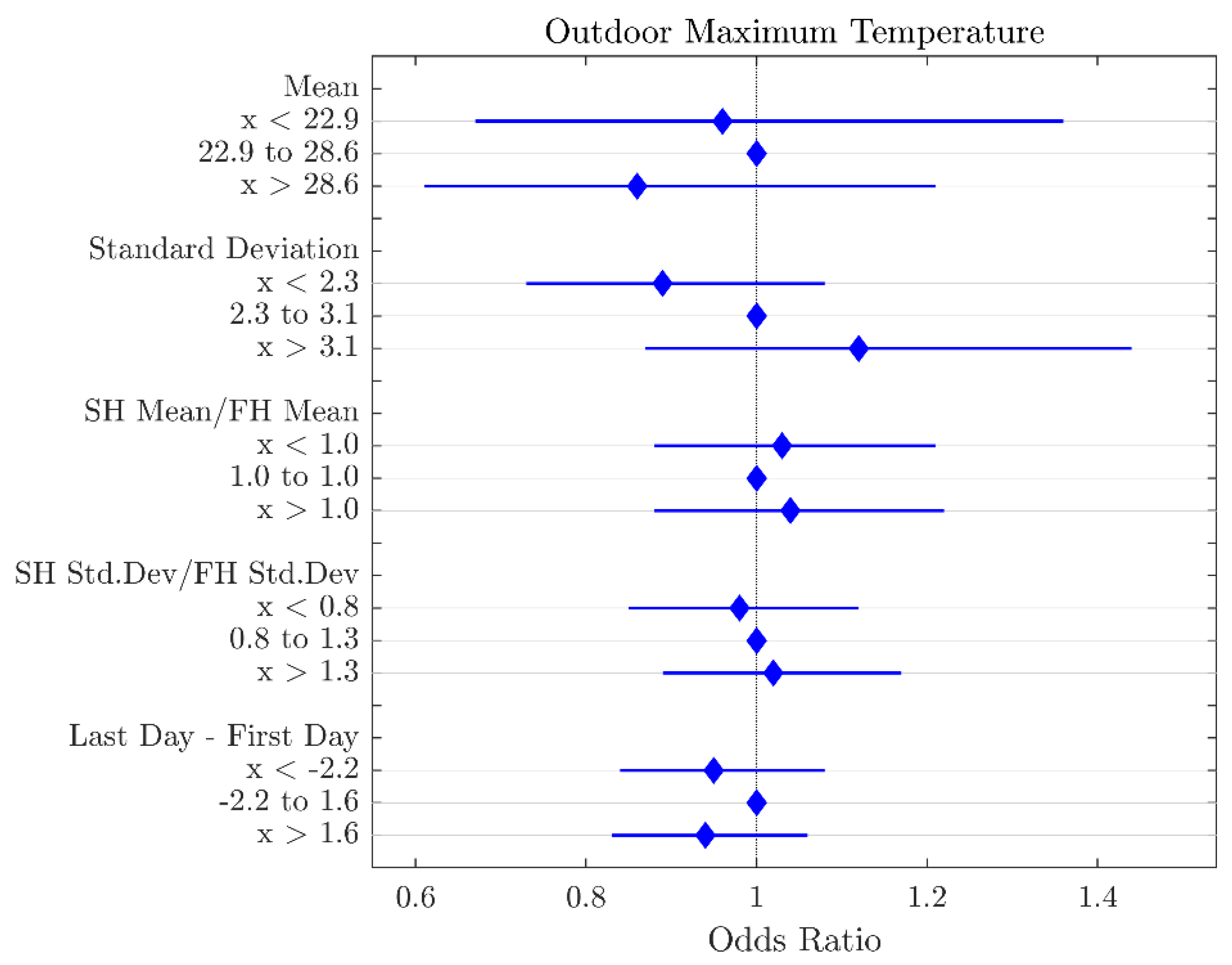
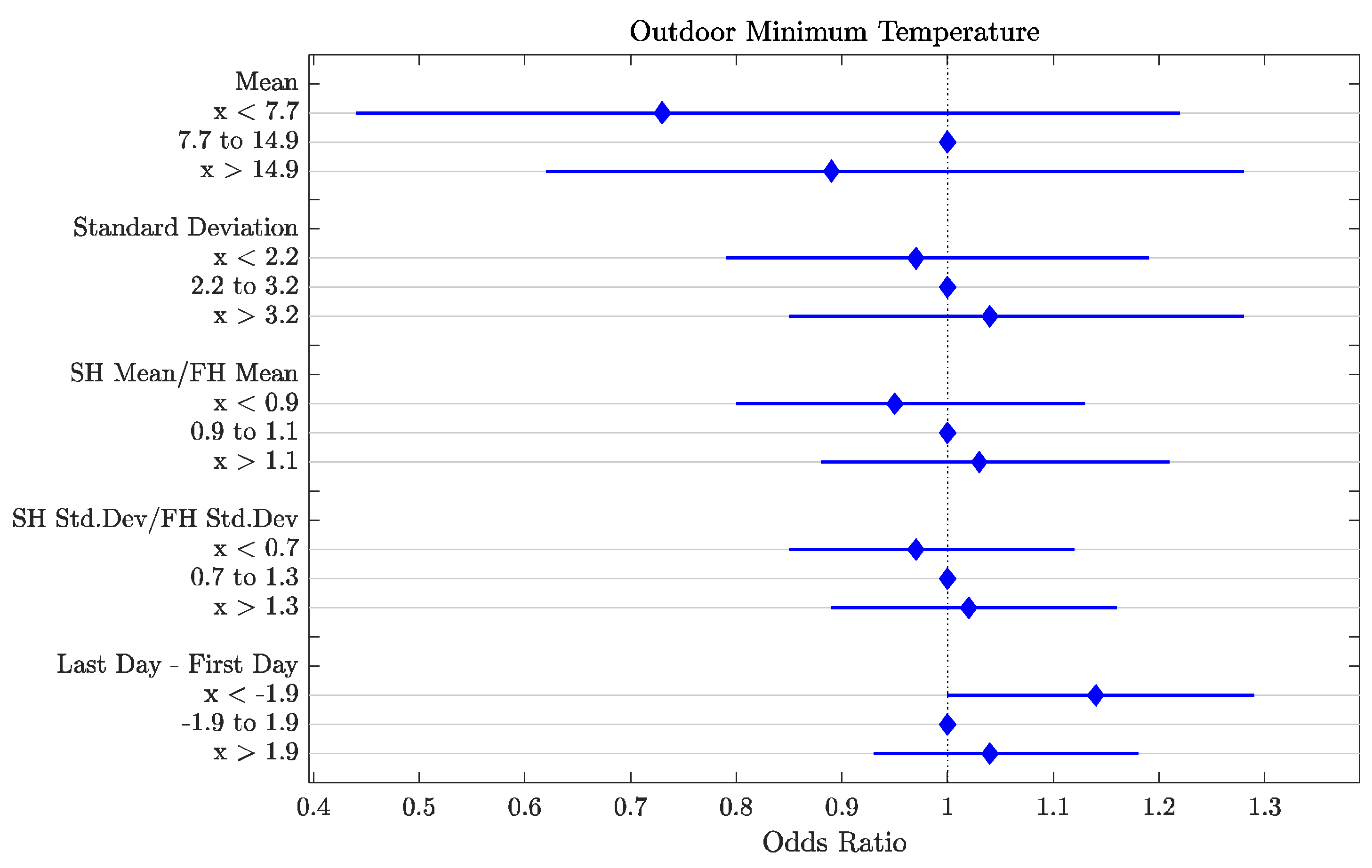
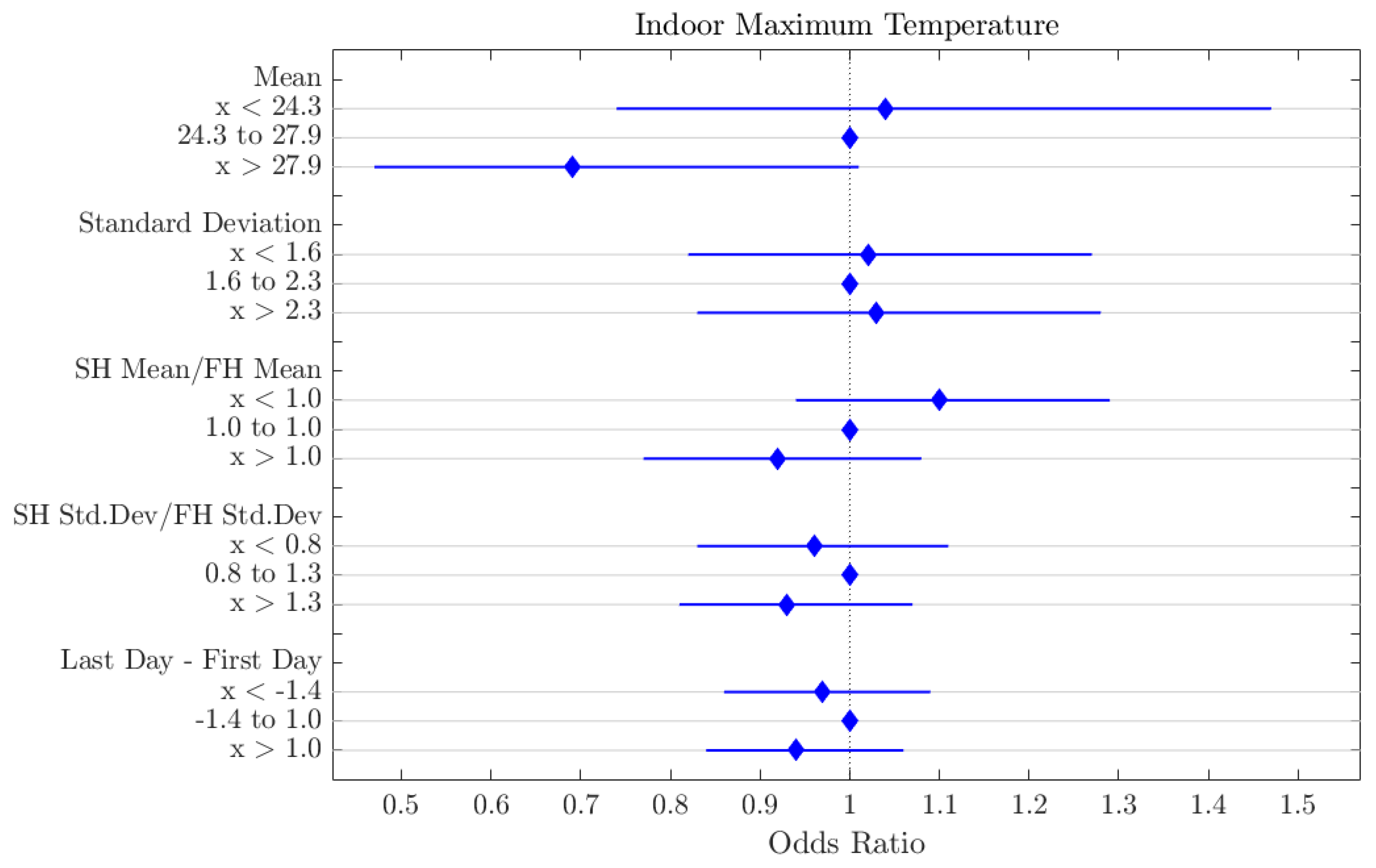
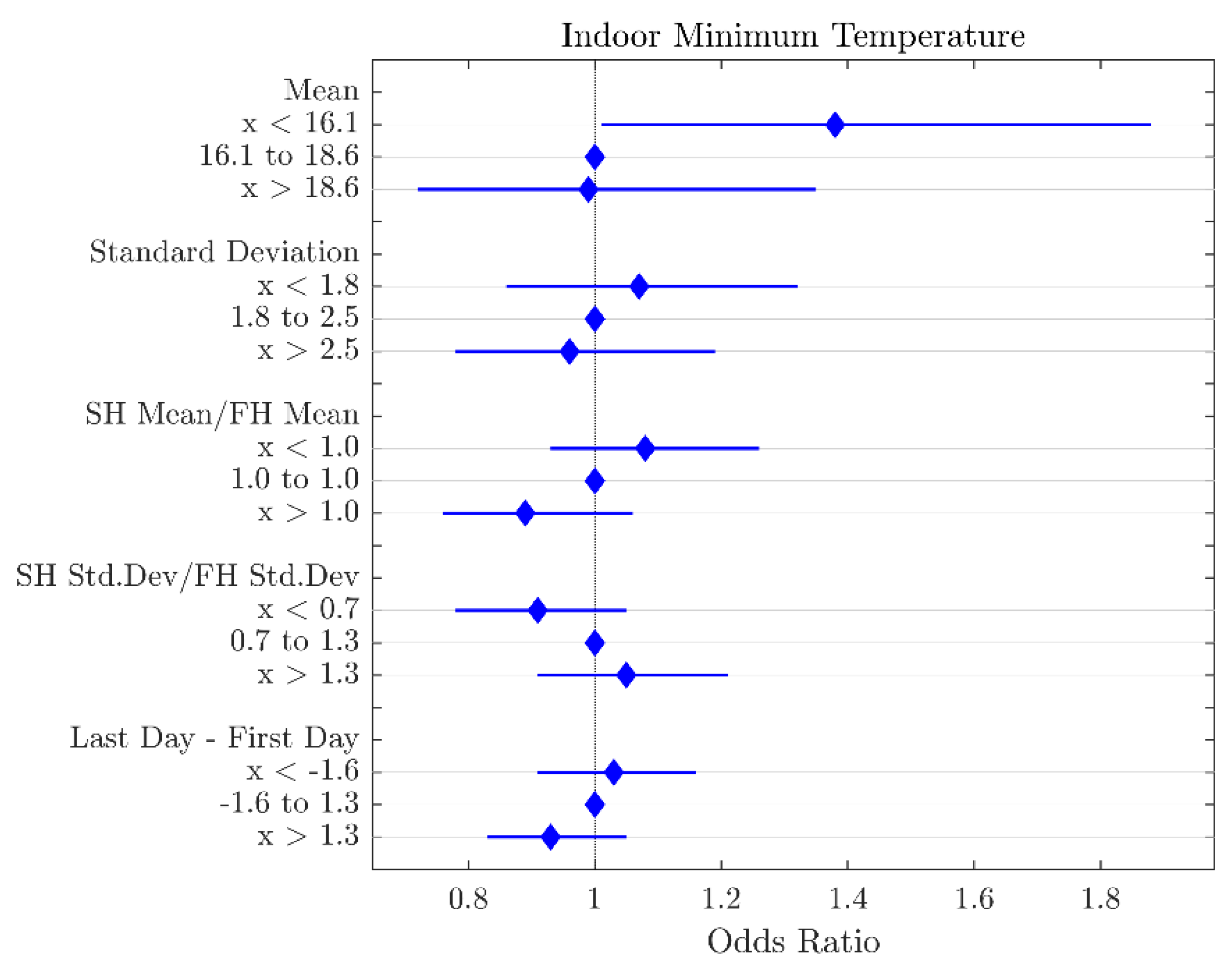
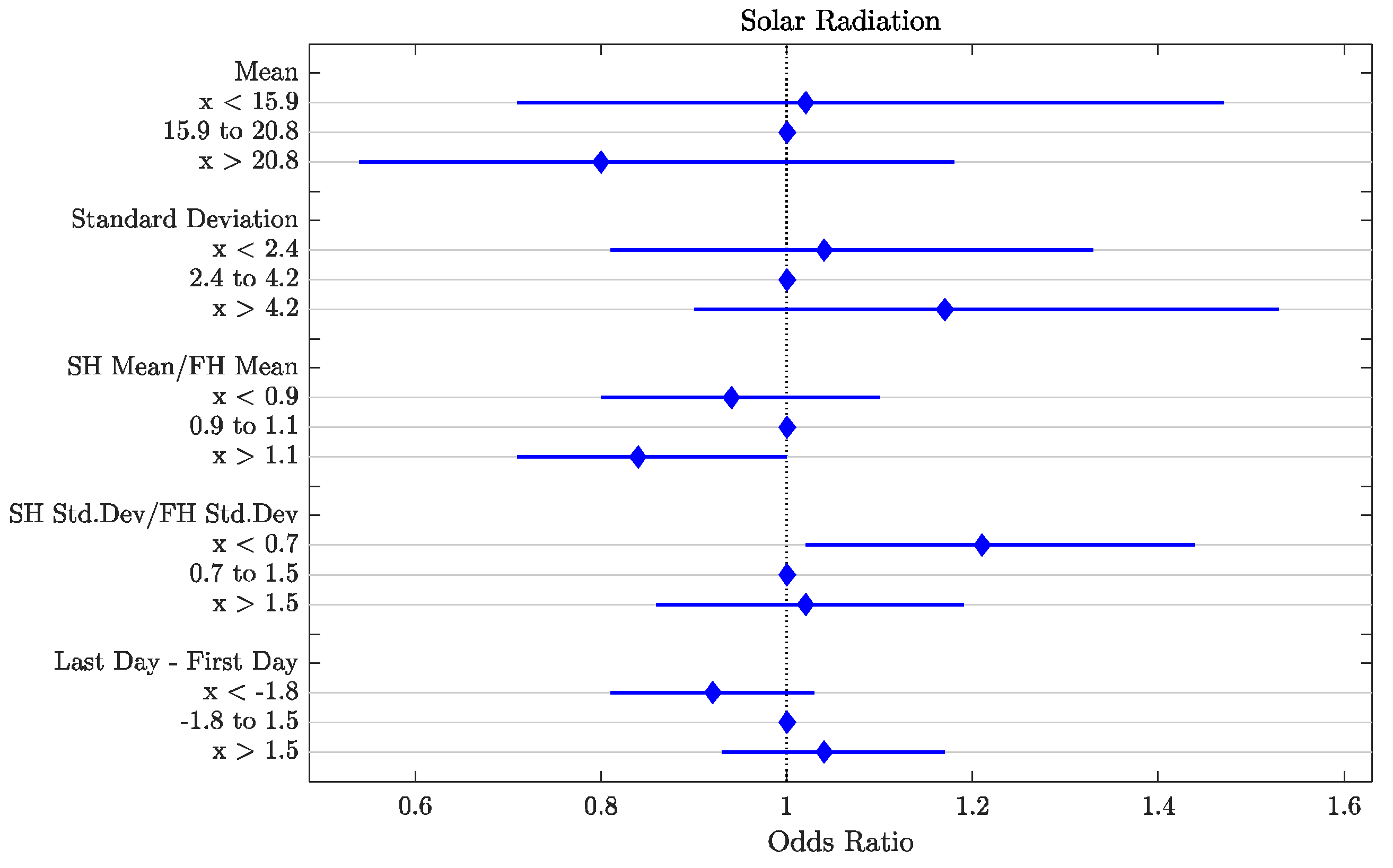
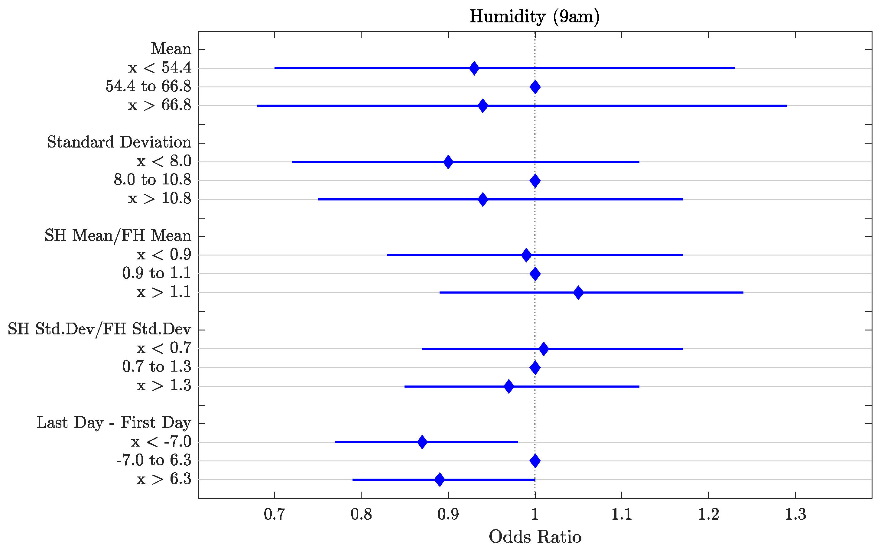
3.2. Environmental Variable Features

Figure 7 plots the odds ratios for the features calculated across the outdoor maximum daily temperature variable. None of the odds ratios calculated across these features were significant at the 95% level. The standard deviation feature shows promising results with the low (<2.3) and high (>3.1) groups exhibiting odds ratios of lower odds (≈0.9) and higher odds (≈1.1), respectively.

Figure 8 plots the odds ratios for the features calculated across the outdoor minimum temperature variable. The only significant result present is the odds ratio (≈1.15/1, p = 0.04) for the low group (<−1.9) of the last day–first day feature. All other features exhibit odds ratios with wide confidence intervals and are not considered significant at the 95% level.

Figure 9 plots the odds ratios for the features calculated across the indoor maximum temperature variable. The results showed that none of the features calculated across the outdoor minimum daily temperature variable exhibited odds ratios that were significant at the 95% level. The high group (>27.9) for the mean feature demonstrates low odds (≈0.7/1, p = 0.06), deviating from 1 by a large margin.

Figure 10 plots the odds ratios for the features calculated across the indoor minimum temperature variable. The low group (<16.6) shows significantly higher odds of a production drop (≈1.4/1, p = 0.04). No other features from this variable demonstrated odds ratios that were significant at the 95% confidence level.

Figure 11 plots the odds ratios for the features calculated across the solar radiation variable. The high group (>1.1) for the SH mean/FH mean feature showed significantly lower odds of a production drop (≈0.8/1, p = 0.04), and the low group SH Std. Dev/FH Std Dev showed a significantly higher risk of a production drop (≈0.2/1, p = 0.03). No other features calculated across this variable produced significant results.

Figure 12 plots the odds ratios for the features calculated across the precipitation variable. The low group (<0.5) for standard deviation exhibited significantly lower odds of a production drop (≈0.6/1, p = 0.04). No other results were statistically significant for this variable; however, the SH mean/FH mean ratio low group exhibited relatively high odds of a production drop (≈1.3/1, p = 0.12).

Figure 13 plots the odds ratios for the features calculated across the humidity (9 a.m.) variable. The last day–first day low group (<−7.0) exhibited significantly lower odds of a production drop (≈0.9/1, p = 0.02). No other results for this variable were statistically significant; however, the last day–first day high group (>6.3) exhibited a promising result with lower odds of a production drop (≈0.9/1, p = 0.06).

Figure 14 plots the odds ratios for the features calculated across the humidity 3 p.m. variable. The low group for the SH mean/FH mean ratio (<0.9) exhibited significantly lower odds of a production drop (≈0.9/1, p = 0.01). No other results for this variable demonstrated statistically significant results.

The results as shown in

Table 3. Summary of significant results for the environmental variables.

Variable	Feature	Group	Odds Ratios	p-Value
Outdoor Minimum Temperature (%)	Last Day–First Day	x < −1.9	1.14	0.02
Indoor Minimum Temperature (%)	Mean	x < 16.1	1.38	0.04
Solar Radiation (MJ/m2/day)	SH:FH Mean Ratio	x > 1.1	0.84	0.04
Solar Radiation (MJ/m2/day)	SH Std. Dev.:SH Std. Dev. Ratio	x < 0.7	1.21	0.03
Precipitation (mm/day)	Std. Deviation	x < 0.5	0.64	0.04
Humidity (9 a.m.) (%)	Last Day–First Day	x < −0.7	0.87	0.02
Humidity (9 a.m.) (%)	Last Day–First Day	x > 0.63	0.89	0.04
Humidity (3 p.m.) (%)	SH:FH Mean Ratio	x < 0.9	0.77	0.01

provide a summary of the significant features derived from the environmental variables linked with short-term egg production losses. Key environmental variables such as indoor/outdoor temperature, humidity, solar radiation and precipitation were identified.

4. Discussion

The results presented in Section 3 demonstrate a range of significant factors related to the risk of egg production fluctuations (i.e., production drops) in the laying rate of free-range hens. These factors are based on data that can be measured by both technologies directly integrated into production systems, or through climatic data obtained from weather monitoring services.

4.1. Production Parameters

The laying rate, feed intake, water intake, and mortality all demonstrated significant associations with increased or decreased risk of a drop in the laying rate. Features that captured changes in the laying rate showed the most significant results. A standard deviation of below 1.4 in the laying rate or an increasing laying rate (captured through the SH: FH mean ratio and last day–first day difference of above 1.1) both showed reduced risk. The laying rate is a multi-faceted predictor that captures a range of events within production. Previous studies have shown that the actual laying rate is a robust predictor of future laying performance. For example, models developed by [15] that were almost entirely based on the laying rate were able to predict production fluctuations.

Feed intake was a strong predictor, where an increasing feed intake (observed through an SH mean/FH mean ratio > 1.0) correlated with a lower risk of a drop in egg production. In our study, the breeds of laying hens focused on were comprised of Lohmann Brown and Hy-Line Brown hybrids. The study by [20] supports the importance of adequate feed intake by laying hens because feed and nutrients have a direct impact on body development, egg production, and gastrointestinal health. Similarly, ref. [17] used feed intake as a predictor within their forecast models, but only used the simple mean within their fuzzy rule-based model. This work builds upon these previous results, demonstrating that the fluctuation in feed intake is an important predictor for egg production that is easily tracked using commercial sensing technologies.

The results for the water intake were less convincing with the only significant results showing that a low SH Std Dev/FH Std Dev (<0.7) was linked with an increased risk of a drop in production. Previous lab-based studies [22,36,37] have shown that feed and water intake (along with other environmental factors) are linked with metabolic function in laying hens and can affect the laying rate. Laying hens consume more water when an egg is laid compared to non-laying days, with daily water intake more than doubling on laying days. Adequate water intake is essential to prevent heat stress and ensure the well-being of laying hens [20].

The mortality rate variable showed relatively weak associations across the calculated features, with the results presenting a counter-intuitive trend. A higher risk of a production drop was observed for lower mortality rates. Typically, higher mortality rates are linked with the incidence of disease and lower egg production rates in a flock. Several studies showed a higher mortality or disease incidence in free-range compared to hens kept inside [18,19]. For example, Spotty Liver Disease can cause significant loss to the free-range hen industry as it can cause up to 10% flock mortalities and a 25% reduction in egg production in flocks experiencing a disease outbreak [38,39]. We present two explanations for this curious result. Firstly, it is possible the forecast interval between the data window and the response day (this is the day following the data window in this study—see Figure 2) was not sufficient to capture the effect of the mortality rate across the data window. It is possible that these effects occur over a longer time scale (e.g., multiple days) and any production fluctuation caused by the changes to the mortality rate may not be observed until multiple days after. Further investigation around the effect of the forecast interval (similar to that presented by [16]) might provide a complete understanding of the associations surrounding the mortality rate. Secondly, while high mortality rates may be linked to lower production rates, it is unclear if they produce the sudden fluctuations in egg production that are the focus of this work. A higher mortality rate within a flock may result in a steady decrease in production rates over time or a lower peak production for the flock. These aspects are not captured by the modeling in this study and warrant further investigation. It should be noted that the study by [15] removed features based on the mortality rate when training models to forecast laying rate fluctuations as they were found to be of less importance. While mortality rates are commonly recorded and available within production datasets, this data item may not be directly usable for forecasting laying rate fluctuations.

4.2. Environmental Parameters

The features calculated from the environmental data demonstrated mixed results in terms of their associations with sudden drops in the laying rate. Many of the features for the outdoor maximum and minimum temperatures produced wide, overlapping, confidence intervals, demonstrating unstable correlations with the response variable. For the indoor maximum temperature, a high standard deviation was associated with a higher risk, while a lower standard deviation was associated with a lower risk. This indicates that variations in high outdoor temperature might be a useful predictor. The outdoor minimum temperature demonstrated a similar, but much weaker trend. We observed in our findings that an increasing minimum temperature (observed through the last day–first day variable) was associated with a lower risk of a production drop. The outdoor minimum temperature demonstrated a similar, but much weaker trend. It can be observed that an increasing minimum temperature (observed through the last day–first day variable) was associated with a lower risk of a production drop. Overall, the treads observed across the outdoor temperature features are consistent with the observations in previous work. Previous studies by [23,24] revealed that high temperatures could cause heat stress in hens thereby reducing feed intake, egg production, and egg quality. Studies done by [40,41] found that high outdoor temperatures of about 33 °C may cause heat stress, which may have an adverse effect on hen-laying performance, resulting in reduced egg production. A similar investigation by [40] showed a reduction in daily feed intake by up to 28.58 g and a reduction in egg production by approximately 28.8% over a 12-day trial period due to heat stress.

The features calculated across the indoor temperature data showed stronger associations than those based on outdoor temperatures. A low mean indoor minimum temperature (<16 °C) was linked with a higher risk of an egg production drop. This result corroborates with the findings of [42] which indicated that decreased ambient temperatures below 18 °C, impacted egg production, egg quality, and feed efficiency in laying hens. The optimal temperature range for hens to ensure good egg production typically falls between 18 °C and 22 °C, as indicated by studies conducted by [43]. It should be noted that the mean indoor and outdoor temperature ranges for the categories differ, reflecting the different distributions of these features. The SH:FH mean ratio feature for the indoor minimum also shows that if the indoor minimum temperature had an upward trajectory, the risk of an egg drop was lower. The indoor temperature feature observations confirmed previous lab-based results that demonstrated that ambient temperatures are an important predictor for laying rates [16]. The indoor temperatures are likely to be more important than the outdoor measurements primarily because free-range hens can choose to move between the two areas and will typically spend more time in the indoor aviary system than exposed directly to the outside environment. Free-range hens spend a substantial amount of time indoors, especially during the night, unfavorable weather conditions, and when seeking feed, water, or nesting areas. Most commercial egg producers are able to actively manage the access to outdoor ranges to manage flock welfare. Consequently, the indoor environment plays a vital role in hens’ productivity. Several features based on the solar radiation, precipitation, and humidity variables demonstrate significant associations with the risk of a production drop. There are limited reports on the direct influence of these features on egg production. According to our findings, a high SH mean:FH mean ratio for solar radiation was associated with a reduced risk of production drops. Increased solar radiation impacts outdoor activities and feed intake of the free-range hens due to higher heat stress which can negatively affect egg production [26,44]. The low standard deviation group for the precipitation variable was associated with a lower risk of a production drop. High rainfall (causing high variation) can cause wet litter leading to the build-up of ammonia thereby, limiting forage activity, and feed intake. These may lead to a decrease in egg production in free-range systems. The results of the humidity at 9 a.m. showed that both lower and higher values of the last day–first day feature for humidity at 9 a.m. were associated with a lower risk of production drops. High relative humidity combined with high temperature can cause heat stress levels and reduce feed intake which can negatively impact egg production [7]. This contradicts the findings presented in [45], where it was found that different relative humidity levels had no effect on egg production and that temperature was a more important contributor to heat stress in laying hens than relative humidity. Overall, the significant associations across these variables produced mixed results that as less well understood when compared to the production variables.

5. Conclusions

This study revealed that production and environmental factors that are measurable through various technologies such as laying rate, feed intake, water intake, and indoor temperatures may be suitable as predictors for production problems. Reduced feed intake was linked with higher risks, but increased water intake was linked with lower risks. Environmental variables like indoor temperatures were also linked with higher risks. The results of this study indicate that production variables provide the strongest correlations with the occurrence of production drops (when compared against the environmental variables), indicating that they are likely more valuable for the task of forecasting. These findings will allow egg producers to understand the impact of feed, water intake, and indoor temperature on egg production ensuring that the laying hens receive balanced diets and adequate temperature thereby improving productivity and preventing economic losses due to short-term egg production fluctuations. This can enable producers to integrate these types of day-to-day data for decision-making to take early proactive measures. Finally, future investigation should be done to evaluate the effects of these kinds of data in machine-learning models to forecast short-term egg drops and laying performance in free-range egg production.

References

1. Bray, H.J.; Ankeny, R.A. Happy Chickens Lay Tastier Eggs: Motivations for Buying Free-range Eggs in Australia. Anthrozoös 2017, 30, 213–226. [Google Scholar] [CrossRef]
2. Pettersson, I.C.; Weeks, C.A.; Wilson, L.R.M.; Nicol, C.J. Consumer perceptions of free-range laying hen welfare. Br. Food J. 2016, 118, 1999–2013. [Google Scholar] [CrossRef]
3. AustralianEggs. Annual Report 2024. 2024. Available online: https://www.australianeggs.org.au/who-we-are/annual-reports (accessed on 26 March 2025).
4. Nicol, C.J.; Potzsch, C.; Lewis, K.; Green, L.E. Matched concurrent case-control study of risk factors for feather pecking in hens on free-range commercial farms in the UK. Br. Poult. Sci. 2003, 44, 515–523. [Google Scholar] [CrossRef]
5. Koch, G.; Elbers, A.R.W. Outdoor ranging of poultry: A major risk factor for the introduction and development of High-Pathogenicity Avian Influenza. Wagen. J. Life Sci. 2021, 54, 179–194. [Google Scholar] [CrossRef]
6. Bestman, M.; Bikker-Ouwejan, J. Predation in Organic and Free-Range Egg Production. Animals 2020, 10, 177. [Google Scholar] [CrossRef]
7. Kim, D.H.; Lee, Y.K.; Lee, S.D.; Lee, K.W. Impact of relative humidity on the laying performance, egg quality, and physiological stress responses of laying hens exposed to high ambient temperature. J. Therm. Biol. 2022, 103, 103167. [Google Scholar] [CrossRef]
8. Abdelqader, A.; Irshaid, R.; Al-Fataftah, A.R. Effects of dietary probiotic inclusion on performance, eggshell quality, cecal microflora composition, and tibia traits of laying hens in the late phase of production. Trop. Anim. Health Prod. 2013, 45, 1017–1024. [Google Scholar] [CrossRef] [PubMed]
9. Zhang, P.; Yan, T.; Wang, X.; Kuang, S.; Xiao, Y.; Lu, W.; Bi, D. Probiotic mixture ameliorates heat stress of laying hens by enhancing intestinal barrier function and improving gut microbiota. Ital. J. Anim. Sci. 2016, 16, 292–300. [Google Scholar] [CrossRef]
10. Nagle, T.A.; Glatz, P.C. Free range hens use the range more when the outdoor environment is enriched. Asian-Australas. J. Anim. Sci. 2012, 25, 584–591. [Google Scholar] [CrossRef]
11. AustralianEggs. Available online: https://www.australianeggs.org.au/farming/egg-quality-standards (accessed on 11 September 2024).
12. Zhai, Z.; Zhang, J.; Chai, X.; Kong, F.; Wu, J.; Zhang, J.; Han, S. A laying hen breeding environment monitoring system based on internet of things. IOP Conf. Ser. Earth Environ. Sci. 2019, 371, 032039. [Google Scholar]
13. BigDutchman. NATURA® Step and Step XL Aviary Systems; BigDutchman: Holland, MI, USA, 2023; Available online: https://www.bigdutchmanusa.com/wp-content/uploads/2023/04/NATURA%C2%AE-Step-and-Step-XL_Eng.pdf (accessed on 24 March 2025).
14. FarmMark. Aviary PRO11; FarmMark: Queensland, Australia, 2023. [Google Scholar]
15. Morales, I.R.; Cebrián, D.R.; Blanco, E.F.; Sierra, A.P. Early warning in egg production curves from commercial hens: A SVM approach. Comput. Electron. Agric. 2016, 121, 169–179. [Google Scholar] [CrossRef]
16. Gonzalez-Mora, A.F.; Rousseau, A.N.; Larios, A.D.; Godbout, S.; Fournel, S. Assessing environmental control strategies in cage-free aviary housing systems: Egg production analysis and Random Forest modeling. Comput. Electron. Agric. 2022, 196, 106854. [Google Scholar] [CrossRef]
17. Omomule, T.G.; Ajayi, O.O.; Orogun, A.O. Fuzzy prediction and pattern analysis of poultry egg production. Comput. Electron. Agric. 2020, 171, 105301. [Google Scholar] [CrossRef]
18. Fossum, O.; Jansson, D.S.; Etterlin, P.E.; Vagsholm, I. Causes of mortality in laying hens in different housing systems in 2001 to 2004. Acta Vet. Scand. 2009, 51, 3. [Google Scholar] [CrossRef] [PubMed]
19. Sherwin, C.M.; Richards, G.J.; Nicol, C.J. Comparison of the welfare of layer hens in 4 housing systems in the UK. Br. Poult. Sci. 2010, 51, 488–499. [Google Scholar] [CrossRef]
20. Bryden, W.L.; Li, X.; Ruhnke, I.; Zhang, D.; Shini, S. Nutrition, feeding and laying hen welfare. Anim. Prod. Sci. 2021, 61, 893–914. [Google Scholar] [CrossRef]
21. PoultryHub. Nutrient Requirements of Egg Laying Chickens. 2024. Available online: https://www.poultryhub.org/all-about-poultry/nutrition/nutrient-requirements-of-egg-laying-chickens (accessed on 14 August 2024).
22. Howard, B.R. Water balance of the hen during egg formation. Poult. Sci. 1975, 54, 1046–1053. [Google Scholar] [CrossRef]
23. Wasti, S.; Sah, N.; Mishra, B. Impact of Heat Stress on Poultry Health and Performances, and Potential Mitigation Strategies. Animals 2020, 10, 1266. [Google Scholar] [CrossRef]
24. Donkoh, A. Ambient temperature: A factor affecting performance and physiological response of broiler chickens. Int. J. Biometeorol. 1989, 33, 259–265. [Google Scholar] [CrossRef]
25. Reece, F.; Deaton, J. Use of evaporative cooling for broiler chicken production in areas of high relative humidity. Poult. Sci. 1971, 50, 100–104. [Google Scholar] [CrossRef]
26. Kim, H.R.; Ryu, C.; Lee, S.D.; Cho, J.H.; Kang, H. Effects of Heat Stress on the Laying Performance, Egg Quality, and Physiological Response of Laying Hens. Animals 2024, 14, 1076. [Google Scholar] [CrossRef] [PubMed]
27. Sampaio, F.B.G.; Passerino, A.S.; Kozicki, L.E.; Weber, S.; Teixeira, V.N.; Pereira, J.F.S.; Segui, M.S. Effect of temperature, air humidity, and rainfall on the reproductive season of Rhea americana (Linaeus, 1758) at latitude 25°S. Der Zoologische Garten 2015, 84, 127–134. [Google Scholar] [CrossRef]
28. Rana, M.S.; Lee, C.; Lea, J.M.; Campbell, D.L.M. Relationship between sunlight and range use of commercial free-range hens in Australia. PLoS ONE 2022, 17, e0268854. [Google Scholar] [CrossRef]
29. Pyrzak, R.; Snapir, N.; Goodman, G.; Perek, M. The effect of light wavelength on the production and quality of eggs of the domestic hen. Theriogenology 1987, 28, 947–960. [Google Scholar] [CrossRef]
30. Hardin, J.W.; Hilbe, J.M. Generalized Estimating Equations; Chapman and Hall/CRC: New York, NY, USA, 2002. [Google Scholar] [CrossRef]
31. Cummins, C.; Welch, M.; Inkster, B.; Cupples, B.; Weaving, D.; Jones, B.; King, D.; Murphy, A. Modelling the relationships between volume, intensity and injury-risk in professional rugby league players. J. Sci. Med. Sport 2019, 22, 653–660. [Google Scholar] [CrossRef] [PubMed]
32. Jaspers, A.; Kuyvenhoven, J.P.; Staes, F.; Frencken, W.G.P.; Helsen, W.F.; Brink, M.S. Examination of the external and internal load indicators’ association with overuse injuries in professional soccer players. J. Sci. Med. Sport 2018, 21, 579–585. [Google Scholar] [CrossRef]
33. Ratcliffe, S.J.; Shults, J. GEEQBOX: A MATLAB toolbox for generalized estimating equations and quasi-least squares. J. Stat. Softw. 2008, 25, 1–14. [Google Scholar] [CrossRef]
34. The MathWorks, Inc. MATLAB, version 9.6.0.1114505 (R2019a); The MathWorks, Inc.: Natick, MA, USA, 2019. [Google Scholar]
35. Bland, J.M.; Altman, D.G. The odds ratio. BMJ 2000, 320, 1468. [Google Scholar] [CrossRef]
36. Petek, M.; Alpay, F.; Gezen, S.S.; Çibik, R. Effects of Housing System and Age on Early Stage Egg Production and Quality in Commercial Laying Hens. Kafkas Univ. Vet. Fak. Derg. 2009, 15, 57–62. [Google Scholar]
37. Li, Y.; Ito, T.; Nishibori, M.; Yamamoto, S. Effects of environmental temperature on heat production associated with food intake and on abdominal temperature in laying hens. Br. Poult. Sci. 1992, 33, 113–122. [Google Scholar] [CrossRef]
38. Grimes, T.; Reece, R. Spotty liver disease–an emerging disease in free-range egg layers in Australia. In Proceedings of the Sixtieth Western Poultry Disease Conference, Sacramento, CA, USA, 20–23 March 2011. [Google Scholar]
39. Crawshaw, T. A review of the novel thermophilic Campylobacter, Campylobacter hepaticus, a pathogen of poultry. Transbound Emerg. Dis. 2019, 66, 1481–1492. [Google Scholar] [CrossRef] [PubMed]
40. Li, G.M.; Liu, L.P.; Yin, B.; Liu, Y.Y.; Dong, W.W.; Gong, S.; Zhang, J.; Tan, J.H. Heat stress decreases egg production of laying hens by inducing apoptosis of follicular cells via activating the FasL/Fas and TNF-alpha systems. Poult. Sci. 2020, 99, 6084–6093. [Google Scholar] [CrossRef]
41. Wu, X.; Zheng, B.; Mei, Z.; Yu, C.; Song, Z.; Sheng, Z.; Gong, Y. Key parameters of physiological responses to acute heat stress in two commercial layers determined by Fisher discriminant analyses. J. Therm. Biol. 2023, 117, 103694. [Google Scholar] [CrossRef]
42. Kim, D.H.; Song, J.Y.; Park, J.; Kwon, B.Y.; Lee, K.W. The Effect of Low Temperature on Laying Performance and Physiological Stress Responses in Laying Hens. Animals 2023, 13, 3824. [Google Scholar] [CrossRef] [PubMed]
43. Paura, L.; Arhipova, I.; Jankovska, L.; Bumanis, N.; Vitols, G.; Adjutovs, M. Evaluation and association of laying hen performance, environmental conditions and gas concentrations in barn housing system. Ital. J. Anim. Sci. 2022, 21, 694–701. [Google Scholar] [CrossRef]
44. de Oliveira, E.M.; de Oliveira, L.Q.M.; do Nascimento Mós, J.V.; Teixeira, B.E.; Nascimento, S.T.; dos Santos, V.M. Solar radiation limits the use of paddocks by laying hens raised in the free-range system. Trop. Anim. Health Prod. 2022, 54, 181. [Google Scholar] [CrossRef]
45. Yahav, S.; Shinder, D.; Razpakovski, V.; Rusal, M.; Bar, A. Lack of response of laying hens to relative humidity at high ambient temperature. Br. Poult. Sci. 2000, 41, 660–663. [Google Scholar] [CrossRef]
Figure 1. An exemplar production egg curve demonstrating the detection of the problematic days using the prominence-based detection algorithm.
Agriculture 15 00743 g001
Figure 2. An outline of the modeling workflow. Starting from the top, the 14-day raw data window was used to process feature data. The data for each feature was binned into tertiles and a generalized estimating equation (GEE) model was trained on each bin. Finally, the odds ratios were derived from the models and plotted using forest plots.
Agriculture 15 00743 g002
Figure 3. The odds ratios for the data features based on the laying rate across the 14-day data window. The mean, standard deviation, and last day–first day are expressed as a percentage (%) as per their underlying data item.
Agriculture 15 00743 g003
Figure 4. The odds ratios for the data features based on the feed intake across the 14-day data window The mean, standard deviation, and last day–first day features are expressed as g/hen/day, as per their underlying data item.
Agriculture 15 00743 g004
Figure 5. The odds ratios for the data features based on the water intake (ml/hen/day) across the 14-day data window. The mean, standard deviation, and last day–first day features are expressed as ml/hen/day, as per their underlying data item.
Agriculture 15 00743 g005
Figure 6. The odds ratios for the data features based on the mortality rate across the 14-day data window. SH mean/FH mean ratio: Second half mean/first half mean ratio. SH Std. Dev/FH Std. Dev: Second half standard deviation/first half standard deviation ratio. The mean, standard deviation, and last day–first day are expressed as a percentage (%) as per their underlying data item.
Agriculture 15 00743 g006
Figure 7. The odds ratios for the data features based on the outdoor maximum temperature across the 14-day window data. SH mean/FH mean ratio: Second half mean/first half mean ratio. SH Std. Dev/FH Std. Dev: Second half standard deviation/first half standard deviation ratio. The mean, standard deviation, and last day–first day are expressed as degrees Celsius (°C) as per their underlying data item.
Agriculture 15 00743 g007
Figure 8. The odds ratios for the data features based on the outdoor minimum temperature across the 14-day data window. SH mean/FH mean ratio: Second half mean/first half mean ratio. SH Std. Dev/FH Std. Dev: Second half standard deviation/first half standard deviation ratio. The mean, standard deviation, and last day–first day are expressed as degrees Celsius (°C) as per their underlying data item.
Agriculture 15 00743 g008
Figure 9. The odds ratios for the data features based on the indoor maximum temperature across the 14-day data window. SH mean/FH mean ratio: Second half mean/first half mean ratio. SH Std. Dev/FH Std. Dev: Second half standard deviation/first half standard deviation ratio. The mean, standard deviation, and last day–first day are expressed as degrees Celsius (°C) as per their underlying data item.
Agriculture 15 00743 g009
Figure 10. The odds ratios for the data features based on the indoor minimum temperature across the 14-day data window. SH mean/FH mean ratio: Second half mean/first half mean ratio. SH Std. Dev/FH Std. Dev: Second half standard deviation/first half standard deviation ratio. The mean, standard deviation, and last day–first day are expressed as degrees Celsius (°C) as per their underlying data item.
Agriculture 15 00743 g010
Figure 11. The odds ratios for the data features based on the solar radiation across the 14-day data window. SH mean/FH mean ratio: Second half mean/first half mean ratio. SH Std. Dev/FH Std. Dev: Second half standard deviation/First half standard deviation ratio. The mean, standard deviation, and last day–first day are expressed as MJ/m2/day as per their underlying data item.
Agriculture 15 00743 g011
Figure 12. The odds ratios for the data features based on the precipitation across the 14-day data window. SH mean/FH mean ratio: Second half mean/First half mean ratio. SH Std. Dev/FH Std. Dev: Second half standard deviation/First half standard deviation ratio. The mean, standard deviation, and last day–first day are expressed mm/day as per their underlying data item.
Agriculture 15 00743 g012
Figure 13. The odds ratios for the data features based on the humidity (9 a.m.) across the 14-day data window. SH mean/FH mean ratio: Second half mean/first half mean ratio. SH Std. Dev/FH Std. Dev: Second half standard deviation/first half standard deviation ratio. The mean, standard deviation, and last day–first day are expressed as a percentage (%) as per their underlying data item.
Agriculture 15 00743 g013
Figure 14. The odds ratios for the data features based on the Humidity (3 p.m.) across the 14-day data window. SH mean/FH mean ratio: Second half mean/first half mean ratio. SH Std. Dev/FH Std. Dev: Second half standard deviation/first half standard deviation ratio. The mean, standard deviation, and last day–first day are expressed as a percentage (%) as per their underlying data item.
Agriculture 15 00743 g014