Abstract
Sorting corn seeds before sowing is crucial to ensure the varietal purity of the seeds and the yield of the crop. However, most of the existing methods for sorting corn seeds cannot detect both varieties and defects simultaneously. Detecting seeds in motion is more difficult than at rest, and many models pursue high accuracy at the expense of model inference time. To address these issues, this study proposed a real-time detection model, YOLO-SBWL, that simultaneously identifies corn seed varieties and surface defects by using images taken at different conveyor speeds. False detection of damaged seeds was addressed by inserting a simple and parameter-free attention mechanism (SimAM) into the original “you only look once” (YOLO)v7 network. At the neck of the network, the path-aggregation feature pyramid network was replaced with the weighted bi-directional feature pyramid network (BiFPN) to increase the accuracy of classifying undamaged corn seeds. The Wise-IoU loss function supplanted the CIoU loss function to mitigate the adverse impacts caused by low-quality samples. Finally, the improved model was pruned using layer-adaptive magnitude-based pruning (LAMP) to effectively compress the model. The YOLO-SBWL model demonstrated a mean average precision of 97.21%, which was 2.59% higher than the original network. The GFLOPs were reduced by 67.16%, and the model size decreased by 67.21%. The average accuracy of the model for corn seeds during the conveyor belt movement remained above 96.17%, and the inference times were within 11 ms. This study provided technical support for the swift and precise identification of corn seeds during transport.
1. Introduction
Corn is recognized as one of the most vital cereals globally and serves as a crucial source of feed for livestock and agriculture [1]. Seeds play an essential role as the carriers of genetic information in crops. However, corn seeds are vulnerable to damage and mildew during storage and transportation, which can considerably reduce the seed sowing quality, thereby affecting the crop yield and leading to economic losses. Surface defects and varietal purity are crucial indicators of seed quality. Traditional seed defect detection methods often rely on manual operation, are inefficient and are prone to subjective factors. Therefore, it is crucial to investigate an objective and automatic identification method for the effective sorting of seeds before sowing, which is essential for ensuring crop yield and enhancing economic benefits [2]. Extensive studies regarding the classification of corn seeds have attempted to overcome such challenges [3,4,5,6].
In recent years, the integration of machine vision with deep learning has seen increasing application [7,8,9,10,11]. Compared with traditional machine learning methods, deep learning decreases the subjectivity of manual feature extraction and automatically extracts various complex features from input data. Altuntaş et al. [12] used VGG19 to differentiate haploid and diploid seeds with up to 94.22% accuracy. Kurtulmuş [13] compared three deep learning models and found that GoogleNet attained the highest classification accuracy of 95% for sunflower seed classification. Zhou et al. [14] designed a method using a convolutional neural network (CNN) to reconstruct pixel spectral images. This method accurately identified the non-embryoid and embryoid forms for six distinct varieties of normal corn seeds with 93.33% and 95.56% accuracy, respectively. Luo et al. [15] compared six CNN models to obtain the best algorithm for intelligently classifying weed seeds. The AlexNet network exhibited high accuracy and a low detection time, while GoogLeNet achieved the best accuracy.
In the sorting preprocessing process of seeds, the classification network mainly classified the regions in the image and determined and output the category label or probability of image. It had fewer levels, lower model complexity and a relatively simple network structure. But it could not accurately localize the seeds and achieve tasks such as seed counting or sorting due to the lack of location information [16,17]. The object detection network solved this problem effectively by involving both location and category information, but it was more complex and required higher computational resources compared to the classification network. A category of classical object detection algorithms is region-based candidate object detection, with representative algorithms including R-CNNs and Fast R-CNNs. An R-CNN uses a selective search method to generate candidate regions, which involves a large number of computations, and each candidate region needs to go through a deep convolutional network for feature extraction, which further increases the computational burden. A Faster R-CNN achieves the fast generation of candidate regions by introducing a region proposal network (RPN), but its overall speed is still relatively slow. This is attributed to the fact that a Faster RCNN remains a two-stage detection algorithm, necessitating the sequential execution of candidate region generation and feature extraction [18]. In industrial inspection, this limits its application to large-scale, high-speed production lines. In contrast to two-stage detection methods, one-stage detection, such as the YOLO series, extracts features directly from the network to predict, classify and regress objects [19]. Using an end-to-end approach, the normalized image is fed directly into the CNN, and the location information and class of the object is predicted via regression, which drastically reduces the latency and computational requirements. YOLO balances accuracy and speed, and this approach is more suitable for inspection in industry. Ouf [20] used transfer learning and CNNs to classify leguminous seeds with different backgrounds, sizes and shapes. YOLOv4 exhibited higher accuracy and detection speed compared with a Faster R-CNN. Shi et al. [21] applied the YOLOv5 series model to identify barley seeds and reported that the accuracy of the mixed dataset using the YOLOv5x6 model was substantially better than that of the single-class dataset. Thangaraj Sundaramurthy et al. [22] used four different variants of YOLOv5 to identify corn seeds that were Fusarium infected from the processing lines. The results showed that the YOLOv5-s model showed the highest mAP@50 of 99% for the detection of Fusarium infection in individual corn grain in images. The YOLOv5-n model performed well, with minimal training time and a higher inference speed for detection in real-time scenarios and videos.
The basic object detection network showed false and missed detection due to its insufficient ability to learn features, a complex detection background or smaller detection object. These cases were verified, and it was demonstrated through experiments that the improvement of the basic network could effectively reduce the number of false and missed detections [23,24]. To enhance the ability of the network to learn and capture features, researchers have opted to incorporate attention mechanisms or substitute the feature network to refine the model. Zhang et al. [25] chose to introduce attention mechanisms in YOLOv5s to enable it to learn features better. The results showed that the CBAM (Convolutional Block Attention Module) accentuated pertinent information critical for coated seed recognition and could extract the features of seeds from images more effectively than the other three attention mechanisms. The improved network achieved the best performance in the self-built coated-seed dataset and increased the mAP value by 1.22% compared with the original model. Zhang and Li [26] incorporated the effective pyramid split attention (EPSA) into the backbone network of YOLOv5s. The results showed that the EPSA module improved the feature extraction ability for small targets with similar backgrounds. The proposed method addressed the problem of difficulty in detecting rape seeds at different key growth stages. Zhao et al. [27] integrated four CBAM attention mechanisms into YOLOv5s and used CARAFE up-sampling to replace the neck of the model. The improved model enhanced the detection precision and achieved effective counting and localization of seed images. Xiao et al. [28] engineered an improved YOLOv5 network to identify damaged Camellia oleifera seeds, incorporating both the BiFPN and CA. The accuracy of the final model was increased by 6.1%.
Although the improved model enhanced the detection precision, it introduced more computing owing to the enormous number of parameters in the deep learning network, leading to slower inference. Optimizing the model to be lightweight is a practical approach for model compression to achieve the real-time standards of industrial detection. Wang et al. [29] designed a pruned YOLOv3 network. The model size after channel pruning was 4.07 MB, with an average accuracy of 98.33%. Furthermore, the model achieved rapid and non-destructive detection of kidney bean seeds. Beyaz and Saripinar [30] classified sugar beet monogerm and multigerm seeds on the NVIDIA artificial intelligence boards. The experimental results proved that the accuracy of YOLOv4-tiny was only a little bit worse than that of YOLOv4, but YOLOv4-tiny had seven more frames per second (FPS) than YOLOv4. This suggested that models with a more simple structure had a significant advantage in terms of inference speed on embedded devices. Xia et al. [31] replaced the backbone of the YOLOv5s with MobilenetV3-Small to detect defects on the surface of corn seeds. The final model size was 8.8 MB, with a detection accuracy of 92.8%. Jiao et al. [32] combined μCT technology with the improved YOLOv7-tiny network to identify invisible internal endosperm cracks in corn seeds produced during the soaking process. This approach extracted crack information accurately and automatically, with a 93.8% accuracy and a 9.7 MB model size. Li et al. [33] addressed problems such as low accuracy on edge location and heavy model parameters in detecting tomatoes by improving and simplifying the YOLOv10 model. The results showed that the parameters and FLOPs of the final model were reduced by 54% and 64.9%, respectively. The above research confirmed that model compression was an effective way to reduce the model size and balance the model computation and detection accuracy.
Currently, the YOLO series has been updated to YOLOv11. Each network in the YOLO series has its own characteristics: YOLOv7 introduces a dynamic label assignment strategy, which improves the training efficiency and detection performance of the model. YOLOv8 introduces a dynamic kernel attention mechanism and anchor-free detection technique, which performs better on tasks in complex scenarios. YOLOv9 uses multi-level auxiliary feature extraction and domain-specific augmentation strategies [34]. YOLOv10 eliminates the traditional non-maximum suppression (NMS). A dual-label assignment strategy is implemented. YOLOv11 introduces the C3k2 module in the backbone network and enhances spatial attention using C2PSA [35]. In tasks with simpler backgrounds such as the real-time detection of seeds on a conveyor belt, a more complex network architecture also means that more computational resources are required. The more simplified architecture of the YOLOv7 network in comparison still achieves excellent performance. The stability and reliability of YOLOv7 has been widely recognized in many real-time inspection tasks. Therefore, exploring practical improvements will more effectively support subsequent deployments.
This study proposed the YOLO-SBWL method, which combines machine vision and deep learning to achieve both the classification of healthy seeds and distinction of damaged seeds during transportation on the conveyor belt. The major contributions include the following: (1) A self-built, real-time image acquisition system was used to obtain a dataset of corn seeds, and data augmentation was performed on the original data to expand the dataset. (2) This study inserted the SimAM into the YOLOv7 network to effectively increase attention to the key features of corn seeds when the texture details of a seed become blurred due to rapid movement and to enhance the recognition accuracy between healthy and defective seeds by assigning weights to each feature. (3) In order to solve the problem of false detection caused by too much similarity between healthy seeds of different varieties, the PAFPN structure was replaced with the BiFPN to enhance the information exchange on different scales and improve the feature fusion ability of the model. In addition, the CIoU loss function was replaced with Wise-IoU to speed up the convergence of the model. (4) The improved model was compressed using the LAMP method and subsequently fine-tuned. This effectively reduced the model size and improved the detection speed.
2. Materials and Methods
2.1. Experimental Sample
The seeds were purchased from the Huiheng seed business department in Harbin, Heilongjiang, China. The producers of the seeds were Fuyu Yinong Seed Industry Co. and Gongzhuling Lvyu Seed Industry Science and Technology Co., both located in Jilin Province, China. This study used 4000 corn seeds of 5 corn varieties as the experimental materials. The five types of seeds were KenNian1, HuangNianZao1, LiangNuo10, HuangNuo6 and LiangNuo58. HuangNuo6 and LiangNuo58 had similar shape appearance, while HuangNianZao1 and KenNian1 were similar in color but smaller in shape. The different types of corn seeds had completely different textures and appearances. The seeds were artificially screened prior to the experiment to remove impurities and seeds unsuitable for the experiment. Each category had three types of defects, including cracks, crush and mold. These categories had different colors, sizes and shapes, which added diversity and complexity. Table 1 lists the names of seeds and the corresponding number of categories.

Table 1.
Quantity of each type of corn seed.
2.2. Image Acquisition
The image acquisition system comprised a camera (MV-CS016-10GC, HIKVISION, Hangzhou, China), a lens (MVL-MF0828M-8MP, HIKVISION, Hangzhou, China), white LED ring light source, conveyor belt, corn seeds and computer (Figure 1). The camera was a 1.6-megapixel CMOS camera with a net-mouth face array, a 1440 × 1080-pixel resolution and a frame rate of 65.2 fps. The camera had a pixel size of 3.45 μm × 3.45 μm. The 1440 × 1080-pixel resolution ensured that the camera was able to cover more details of the seeds. The frame rate of the camera met the real-time requirements of industrial inspection. It was chosen because it is an industrial camera that performs well in terms of image detail and capture speed, and its application is in the field of industrial detection for machine vision [36]. Additionally, it supports a Gigabit Ethernet interface, characterized by high speed, high stability and high resolution. These characteristics were essential for the real-time capture of rapidly moving seed images. The exposure time of the camera in this experiment was set to 3500 microseconds in normal mode.
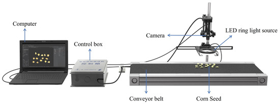
Figure 1.
Image acquisition system.
The seeds were placed randomly on the conveyor belt to avoid contact and overlap. The dimensions of the conveyor belt were 1000 × 365 × 70 mm (length × width × height), with a roller diameter of 57 mm and reduction ratio of 46. The motor controller was connected to the computer using RS485 serial communication, and the speed of the conveyor belt was controlled using the computer. The conveyor speed was adjustable in the 0.0–0.3-m·s−1 range. This range was limited by the equipment, and the maximum adjustable speed was 0.3 m·s−1. For instance, Wang et al. [37] set the conveyor speed to 0.09 m·s−1, and Zhao et al. [27] stated in their experiment that the conveyor speed could be adjusted within the range of 0.0–1.5 m s−1. Similarly, to maximize the utilization of the hardware, the conveyor speed was averagely quantized into 5 levels within its maximum range and converted into rpm for control in this experiment.
2.3. Dataset Processing and Annotation
The images included in the dataset used in the study were captured during the motion of the conveyor belt and collected in May 2024. The dataset comprised images captured at different conveyor belt speeds with an equal number of pictures at each speed to ensure data balancing and avoided bias due to the different number of images at each speed. During image acquisition, the images were captured frame by frame to guarantee all types of seeds were captured in the shots at each speed. The other external environmental factors, such as background, light intensity and camera height, remained settled. The captured images were saved in the JPG format, and the repeated images were removed. Overall, 1180 images were selected, and the training set/validation set/test set ratio was 8:1:1. The training set, validation set and test set for each of the five speed categories contained 188, 24 and 24 samples, respectively.
In this study, LabelImg was selected as a tool for image annotation. Its main function was to label rectangular bounding boxes, and it supported saving labels to multiple formats, which was sufficient to meet the needs for labeling independent seeds (Figure 2). Each seed was designated a corresponding bounding box to ensure all pixels were completely enclosed within the rectangular area. The four points on each bounding box represented the coordinate information of the enclosed seed. The label files were saved in TXT format. However, the tasks, such as polygons or 3D objects, could not be addressed by using LabelImg, compared to more advanced annotation tools, such as LabelMe [38], CVAT [39] and VoTT [40].
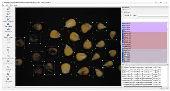
Figure 2.
Data annotation.
2.4. Data Augmentation
Data augmentation was used to extend the dataset in this study, enrich the image dataset and reduce data overfitting [41]. Data augmentation effectively expanded the data, making the sample data more diverse due to the small dataset. The data augmentation techniques included contrast enhancement, horizontal mirroring, vertical mirroring, adding Gaussian noise and brightness enhancement (Figure 3). Among them, brightness and contrast were enhanced by 50% of the original image, respectively. The noise value for adding Gaussian noise was set to 0, with a standard deviation of 0.5. Horizontal mirroring and vertical mirroring were obtained by flipping horizontally and vertically.
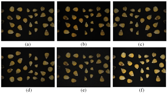
Figure 3.
Examples of corn images: (a) original image, (b) contrast enhancement, (c) horizontal mirroring, (d) vertical mirroring, (e) Gaussian noise and (f) brightness enhancement.
Contrast enhancement made the light and dark areas of an image more distinct by adjusting the distribution of pixel values in the images. This adjustment process could significantly enhance the details and clarity of the image for subsequent analysis and processing. Horizontal mirroring and vertical mirroring increased the diversity of the data and effectively expanded the dataset. The addition of Gaussian noise could simulate the various disturbances that might be encountered in the real world, enhancing the robustness and generalization ability of the model. Brightness enhancement could simulate different lighting conditions at the time of shooting. Finally, the expanded dataset contains 5900 images.
2.5. YOLOv7 Network Architecture
The YOLO series exemplifies one-stage object detection algorithms, achieving end-to-end detection through a singular CNN. With the iteration of the YOLO series, the model complexity and network structure gradually increases. It requires a large amount of training data to adequately train the network, which is a limitation for some application scenarios, as collecting a large amount of well-labeled training data is a time consuming and costly process. However, in the task of detecting corn seeds in real time, a more stable network brings stability to the task, and with the continuous improvement of the YOLO series, YOLOv7 strikes a good balance between accuracy and detection speed. Similar to the detection approach of the YOLOv4 and YOLOv5 models, YOLOv7 comprises an input, backbone, head and prediction.
Figure 4 shows the model structure of YOLOv7. The input module resizes the image to a consistent pixel dimension, aligning with the size requirements of the backbone network, thus minimizing computational complexity [42]. The backbone module comprises CBS, ELAN and MP structures. Among them, the CBS is constituted of a two-dimensional convolutional layer, a batch normalization (BN) layer and SiLU activation function. The ELAN module is constituted of multi-branch convolution and is mainly used to enhance the feature representation of the CNN. The MP module comprises Maxpool and a CBS structure. The feature extraction module is constituted of a PAFPN structure. The head module contains the REP and CBM structures. The CBM module comprises a convolutional layer, BN and sigmoid activation function.
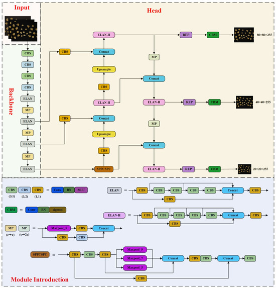
Figure 4.
Model structure of YOLOv7.
2.6. Improvement to YOLOv7
Herein, the corn seeds were categorized into five and three groups based on varieties and defects, respectively. The high similarity between the color and shape of corn seeds meant that their features in the images were blurred owing to the relative motion during the rapid movement of the conveyor belt. Therefore, it was difficult to achieve the expected result by directly using the YOLOv7 basic network. To enhance detection outcomes, the YOLOv7 network underwent modifications to better align with the research needs.
2.6.1. Introduction of Attention Mechanism
In practical industrial applications, selecting an appropriate attention mechanism is vital for boosting the efficiency and performance of the network. False and missed detection of seeds inevitably occurs in the production line. This study chose to insert an attention mechanism into YOLOv7 to strengthen the attention to feature information of corn seeds. SENet stands as a quintessential example of channel attention mechanisms, which calculate the channel attention by 2D pooling and can considerably improve the performance of current mainstream network models [43]. Subsequently, Woo et al. [44] reported that spatial information is important for capturing objects in vision tasks. As a result, the CBAM is proposed; unlike the SENet, the CBAM concatenates channel attention with spatial attention and utilizes convolution to calculate spatial attention. The performance of the model can be enhanced to some degree by inserting this attention mechanism.
However, spatial attention computed via convolution can only extract partial information and fails to build the interdependency necessary for vision tasks. The spatial attention mechanism focuses on the spatial locations on the feature map and generates a spatial attention map by capturing the spatial information of each channel. However, when features become blurred, the difference in information on spatial locations may diminish, making it difficult for the spatial attention mechanism to accurately distinguish between features at different locations. Existing spatial attention mechanisms usually generate attention mappings based on fixed rules or patterns and lack dynamic adaptability to different scenes and features. Therefore, Yang et al. [45] proposed a simple and parameter-free attention mechanism called the SimAM. This module is based on a neuroscience theory, referring to the principle that channel attention and spatial attention work in concert in the human brain, and the module designs an energy function specifically to assess the weight of each discrete neuron, not just connecting the two in series or parallel (Figure 5). It fully utilizes the weight information from all neurons without introducing any additional parameters, thereby ensuring operational efficiency [46].
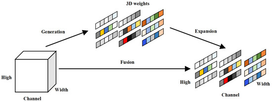
Figure 5.
Structure of the SimAM module.
In the SimAM, if a neuron contains abundant information, it will exhibit distinctive firing patterns compared to its surrounding neurons, effectively suppressing them. Consequently, neurons demonstrating spatial suppression should be prioritized. The energy function of activated neuron is defined using the Formulas (1)–(3):
where is the linear transformation of t; is the linear transformations of xi; t is the target neuron of the input feature in a single channel; xi is the neuron other than the target neuron; and M is the number of neurons in the channel. The energy function is finally given by Formula (4).
The solutions of wt and bt can be obtained using the following formulas:
The minimum energy equation can be derived using Formula (9):
From Formula (9), the less energy a neuron possesses, the more pronounced its distinction from surrounding neurons, making it more significant. Compared with other attention mechanisms, the SimAM can obtain three-dimensional attention weights from the input feature maps. The damaged seeds were distinguished more accurately by introducing the above three attention mechanisms before and after the feature extraction network; the added positions were called Block1 (B1) and Block2 (B2) (Figure 6). The recognition results of the three attention mechanisms added at the above positions were compared in the experiments.
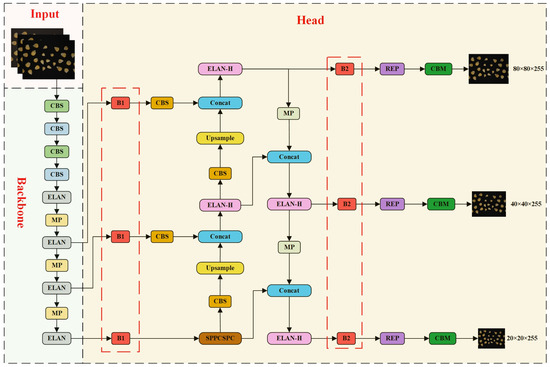
Figure 6.
Position introduced by the attention mechanism in YOLOv7.
2.6.2. Improved PAFPN for Enhancing Feature Fusion
The FPN was a multi-scale feature fusion technique. It seamlessly integrated features from various levels via top–down pathways and lateral connections. FPN effectively combined high-level and low-level semantic information. However, anchor boxes were generated for multiple feature maps in the process of feature fusion, which greatly affected the detection speed. Repeated fused features also affect the feature representation of the model.
The PAFPN used in YOLOv7 adds bottom–up paths on top of the FPN, improving the positional accuracy of the entire feature pyramid without affecting the location information of the fused feature map. However, adding such a path means that the network has to perform additional up-sampling, down-sampling and feature fusion operations. These additional computational steps increase the overall computational cost.
Compared to the PAFPN, the BiFPN removes nodes with only one input and integrates skip connections, which enable direct feature transmission across different layers. It reduces the redundancy of information due to the repeated fusion of features and makes the utilization of features more efficient. Figure 7 shows the structures of the FPN, PAFPN and BiFPN. The reason for selecting the BiFPN to replace the FPN in this paper was due to the diverse shapes and sizes of corn seeds detected in images, which generated input features at various resolutions during training, each contributing differently to the output features. The BiFPN addressed this issue by incorporating an additional weight to adjust for the contribution of various input features on the output features. The BiFPN outperforms the PAFPN by simplifying the structure of the PAFPN to some extent and reducing feature fusion operations and network parameters. However, compared to the structure of the FPN, the BiFPN is still more complex.
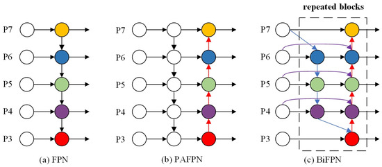
Figure 7.
FPN, PAFPN and BiFPN structures.
2.6.3. Improvements to the Loss Function
The loss function significantly impacts the accuracy of predictions and the effectiveness of the model. In the YOLOv7 network, it comprises confidence, coordinate and classification losses [47]. The original loss function CIoU of YOLOv7 was more concerned with the overlap area, distance from the center point and aspect ratio. As the conveyor speed increased, the distinction between the moldy corn seeds and the background became indistinct, which caused the predicted boxes to appear at different locations from the ground truth boxes, affecting the stability of the model and increasing the training burden.
The Scaled Intersection over Union (SIoU) redefined the penalty metric by considering the vector angle between desired regressions, which mainly addressed the bias of traditional IoUs in target scale changes. It was more focused on scale matching, but the performance was not flexible when the SIoU dealt with small differences in the object.
In cases where the object boundary was not clear enough, the image quality was affected as the conveyor belt ran. It affected the quality of the samples in the dataset. The CIoU and SIoU loss function failed to consider the balance between different quality samples. Therefore, this study replaced CIoU with Wise-IoU based on a dynamic, non-monotonic focusing mechanism [48]. The formula is as follows:
where RWIoU amplifies LIoU of the common-quality anchor box; and LIoU reduces RWIoU of the high-quality anchor box. β is the outlier degree of the anchor box; r is a non-monotonic focus factor. In the smallest box encompassing both the predicted box and the ground truth box, Wg represents the width, and Hg denotes the height.
2.7. Model Pruning
The improved model often fails to achieve the desired results regarding the inference time because of the large amount of complexity and number of parameters of the YOLO network. Compared to simply replacing a lightweight backbone, channel pruning achieves a better balance between accuracy and model size, facilitating easier deployment on embedded devices or small computing platforms. The principle of the channel pruning algorithm involves identifying and eliminating irrelevant network channels and their associated input–output relations [49,50]. Consequently, this study applied the LAMP score within the channel pruning algorithm to prune the enhanced YOLOv7 network. This score is the basis for deciding whether to keep the structure of that channel during the pruning process; it is the magnitude or absolute value of the weights [51]. In neural networks, the weight of each connection determines the importance of the input signal, and the principle of the LAMP score is based on calculating the square of the magnitude of the weights of the target connection and normalizing it to the sum of the squared weight magnitudes of all the surviving weights in the same layer. Assuming that the weight term satisfies u < v, i.e., W[u] < W[v], the formula for LAMP score is as follows:
where u and v denote the index mapping of the weights in ascending order, respectively. W[u] and W[v] denote the weight mapped by indexes u and v, respectively. According to Formula (15), the larger the weight, the larger the corresponding LAMP score. Weights with lower scores are less important and can be pruned.
The two specific steps of pruning the network in this study were included as follows:
- The improved model was pruned to eliminate connections with lower LAMP scores.
- Fine-tuning the pruned model was crucial to mitigate any potential performance degradation during the pruning process.
2.8. Model Evaluation Metrics
The performance of the model was verified by adopting five evaluation criteria, including the precision, recall, F1 score, mAP value and the detection time. The calculations of the precision, F1 score, recall and mAP are expressed as Formulas (16)–(19):
where the mAP is the mean of the average precision (AP) when corn seeds are detected; a higher value means a better detection result for corn seeds. FP, FN and TP are the numbers of false positive, false negative and true positive cases, respectively.
3. Results and Discussion
3.1. Experimental Environment and Parameter Settings
The training and testing processes of the model were performed using the Windows 11 operating system, and the graphics card model was NVIDIA GeForce RTX 3060. The models run on PyTorch 1.12.1, CUDA 11.6 and Python 3.8.16. Hyperparameters need to be set before model training. Adequately setting hyperparameters can significantly enhance the training efficiency of the network. Table 2 lists the final hyperparameters of the model.
Table 2.
Hyperparameters for model training.
YOLOv7 used the One Cycle learning rate policy [52]. In Table 2, lr0 is the initial learning rate; lrf is the final One Cycle learning rate ratio, with the final learning rate denoted lr0 × lrf. The initial learning rate of 0.01 typically provides a modest update step, allowing the model to converge quickly in the early stages of training while avoiding training instability due to too large of a learning rate. weight_decay denotes the weight decay coefficient, being generally set between 0.0001 and 0.001 to prevent model overfitting. warmup_bias_lr, warmup_momentum and warmup_epochs represent the initial learning rate of the bias, momentum and epoch at the initial warmup before training, respectively. box represents the average loss value of the bounding box predicted by the model. cls is the average loss value of the category predicted by the model, which reflects the error between the target category predicted by the model and the actual category. cls_pw is the weight of positive samples in categorization, which measures the inconsistency between the categories predicted by the model and the actual categories. anchor_t is a threshold for determining which anchor sizes should be used to predict a target of a particular size. obj represents the average loss value of objectness predicted by the model. obj_pw is the weight of positive samples in object existence. The resolution of the image was directly adjusted to 640×640 during the input process to the network. The parameters used in this study were referred to the official default parameters of YOLOv7 [53]. The validity of the parameter selection was further verified during the experimental section by comparing the performance of the model by adjusting different learning rates.
3.2. Comparison Experiment Before and After Data Augmentation
To evaluate the effectiveness of data augmentation in the model, Figure 8 showed the training and validation loss curves before and after data augmentation.
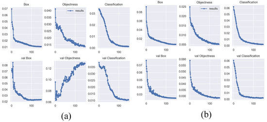
Figure 8.
The results of the model before and after data augmentation. (a) The results before data augmentation. (b) The results after data augmentation.
As shown in Figure 8, before data augmentation, the validation loss curve showed an increasing trend, while the training loss decreased in the model. This indicated that data overfitting existed due to the low complexity of the dataset, and the dataset number was less. After data augmentation, the dataset was extended effectively. The data became more diverse. As a result, the validation loss curve converged more quickly and stabilized, effectively addressing the overfitting of the model.
3.3. Training Results of the YOLO-SBWL Model Under Different Initial Learning Rates
To validate the effectiveness of the learning rate selection, the performance of the model was compared by using different learning rates, as shown in Table 3. Initial learning rates of 0.1, 0.01 and 0.001 were set, and the other parameters were kept constant to maintain consistency in the model.
Table 3.
The training results of the model at different learning rates.
Table 3 showed that the model with an initial learning rate of 0.01 achieved the highest mAP and the lowest validation loss. A smaller learning rate increased the training time and convergence time of the model. Due to the dataset in this experiment being not a large dataset, it was not suitable. On the other hand, the high learning rate made the model take too large of a step at each weight update, and the gradient value of the model became larger, leading to unstable model weights. Therefore, it is reasonable to set the hyperparameters in this way, based on experiments and other published works [54,55,56].
3.4. Comparative Experiments Introduced Attention Mechanisms
Table 4 lists the performance results of the three attention mechanisms placed at different positions in the original network. Based on the comparative experiments, inserting an attention mechanism at position B1 resulted in an overall improvement in parameters such as the accuracy, recall, F1 score and detection speed compared with when it was placed at position B2. The CBAM and SimAM introduced in this model enhanced the detection accuracy of the model, but the SimAM module did not introduce any additional computational complexity on this basis. Overall, introducing the SimAM at the B1 position in the YOLOv7 network was the most effective.
Table 4.
Comparison of three attention mechanisms introduced at different locations.
In order to visually assess the effectiveness of introducing different attention mechanisms at different locations, the Grad-CAM method [57] was used to generate heat maps and analyze the focal region of the model to determine whether it was learning the correct feature information. As shown in Figure 9, the more prominent the red part of the heat map, the higher degree of attention to the part.
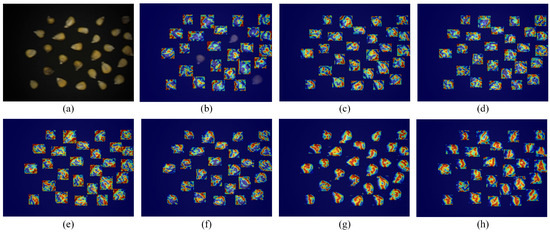
Figure 9.
Grad-CAM heat maps: (a) original image. (b) YOLOv7. (c) B1 position + SE. (d) B2 position + SE. (e) B1 position + CBAM. (f) B2 position + CBAM. (g) B1 position + SimAM. (h) B2 position + SimAM.
Figure 9a is one of the images of corn seeds captured on the conveyor, and it contains different types of seeds. From this figure, the features of the seeds in motion became less distinct, and the differences in features were smaller. Figure 9b shows that the original YOLOv7 network experienced missed detection in detecting corn seeds. There were fewer red regions, which were less capable of learning the features. And the missed detection was solved by introducing the attention mechanism, which was based on the principle of enabling the model to selectively focus on the key parts of the input data. Specifically, Figure 9c,e,g had a stronger ability to pay attention to features than Figure 9d,f,h. It verified that the introduction of the attention mechanism at the B1 position was a reasonable choice.
Additionally, the red regions of Figure 9g,h focused more on the seeds themselves, while the other figures focused more on the edges of the seeds or other positions. In other words, the SE attention mechanism and CBAM tended to over-focus on the features with low importance, while the SimAM improved the focus on the key feature areas of the object by assigning weights to different features. It allowed the network to dynamically adjust its focus, helping it to recognize and localize the presence of objects despite difficultly to distinguish details. Assigning attention weights to each feature takes into account information not only in the channel dimension but also in the spatial dimension. Under dynamic conditions, the attention in the image may change with the movement of the target, deformation and other factors. The SimAM can adaptively adjust the allocation of attention so that the model pays more attention to the important regions.
3.5. Ablation Experiments
This study used ablation experiments to assess each improvement strategy and verify the effectiveness of the improvement strategies. The three improvement methods were combined based on the original network, and the models were trained separately without changing other environments and parameters.
In the test experiments, the dataset was utilized, and the experimental environment remained unchanged. Figure 10, Figure 11 and Table 5 present the results of the ablation experiments. After introducing the SimAM, the mAP improved by 1.85%, and the precision improved by 2.31% (Table 5). After replacing the BiFPN structure on this basis, the mAP improved by 1.42%. The above-mentioned improvement strategies increased the accuracy of the model, owing to enhancing representation and fusion capabilities of the feature maps. The Wise-IoU loss function replaced the original loss function, and the model performance was further improved. The results of all improvements are shown in Figure 10, the prediction boxes for each category are shown in a different color and the reduction in the overall false detection rate after the model improvement proves the effectiveness of the improvement.
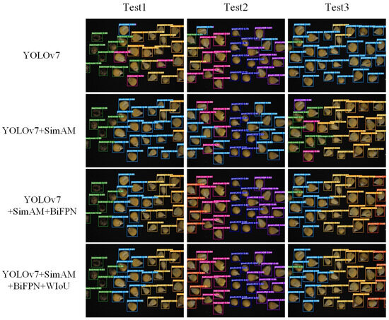
Figure 10.
Detection results of the different improvement strategies.
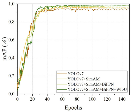
Figure 11.
mAPs of the ablation experiments.
Table 5.
Ablation experiments.
In terms of model size, the flexible adjustment in the number of channels due to the BiFPN structure using 1 × 1 convolution allowed the feature map dimensions at each scale to be upscaled or downscaled as needed. The change in the number of channels of the model after replacing the BiFPN structure was shown by the reduction in the model volume by 1.84 MB, and the computational complexity was reduced accordingly compared to the PAFPN. Regarding the detection speed, the inference time increased by 0.55 ms after inserting the SimAM module, which was within the allowable range. The convergence of the model was accelerated due to simplifying the feature extraction part. Compared to the original network, the detection time of the final model was reduced by 3.02%. The results indicated that after integrating the BiFPN structure and adding the SimAM module, the mAP curve showed a gradual increase beyond 70 iterations, in contrast to the model that incorporated only the SimAM module (Figure 11). Based on these results, the model replaced the Wise-IoU loss function, the convergence speed of the mAP curve did not reduce, and the mAP increased from 97.89% to 98.8%. The inference time was 16.36 ms, which still met the demand for real-time detection.
3.6. Comparison Between Wise-IoU and SIoU
In order to evaluate the effectiveness of the Wise-IoU loss function, under the same experimental conditions, this experiment compared the convergence speed and performance of the analytical model by replacing different loss functions after introducing the SimAM and replacing the BiFPN module.
As shown in Figure 12, the loss values of all models gradually decreased as the number of training sessions increased, indicating that the models were gradually learning the features of the data and optimizing their predictive capabilities. Secondly, Wise-IoU showed a faster rate of decline at the beginning of training and maintained a lower loss value throughout the training process. This suggested that the dynamic, non-monotonic focusing mechanism of Wise-IoU could better guide the model to learn the features of the data during the optimization process and promoted the model to improve the localization accuracy, especially for those objects with a small IoU value.
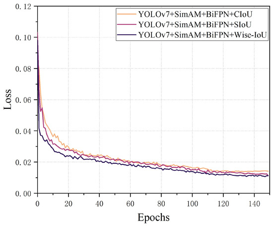
Figure 12.
The loss functions of CIoU, SIoU and Wise-IoU.
3.7. Model Pruning Experiment
The improved model was pruned after training, and then the pruned model was fine-tuned. For a clear comparison, different networks were generated by changing the pruning rates. Table 6 lists the specific experimental results. It was not advisable to set the high pruning rates directly in the model pruning experiments. The pruning rates could be adjusted or stopped in the pruning process to observe the changes in model performance more clearly. The decline in the mAP value indicated that the model performance was affected as the pruning rates increased. Higher pruning rates resulted in more parameters or connections being removed from the model, potentially disrupting the original structure. Figure 13 shows the confusion matrices of models with pruning rates of 0.67 and 0.75, respectively. The darker color of the matrix indicates a higher probability of prediction, and the darker color of the matrix block on the diagonal represents a higher accuracy in the model’s identification. Figure 14 shows the relation between pruning rates and the mAP, model size and inference time. As the pruning rates increased, the inference time, calculations and model size gradually decreased, and the mAP fluctuated as the pruning rates increased.
Table 6.
Comparison of the different pruning rate parameters.
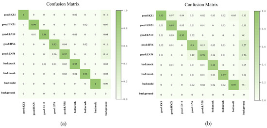
Figure 13.
Confusion matrix for different pruning ratios: (a) the pruning rate of 0.67; (b) the pruning rate of 0.75.
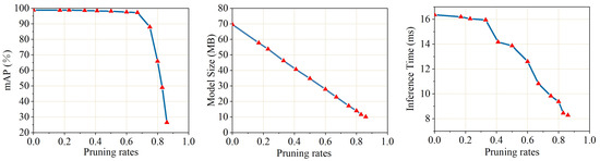
Figure 14.
Model analysis under different pruning rates of the network, measured in terms of the mAP, model size and inference time.
Figure 13a showed that the color of the diagonal matrix blocks was relatively darker. Misclassification existed but was not prevalent. It had a higher probability of prediction accuracy for each category. After increasing the pruning rates, the misclassification cases in Figure 13b increased significantly and subsequently affected the mAP value of the model. Therefore, it was very important to choose an appropriate pruning rate, and the principle of choosing the pruning ratio was to maximize the mAP value as much as possible. In this study, a pruning ratio of 0.67 was finally chosen, at which time the mAP value reached 97.21%, and then decreased rapidly. After pruning, the number of channels decreased significantly (Figure 15). This suggested that such a channel pruning approach was an effective means of simplifying the YOLO series network.
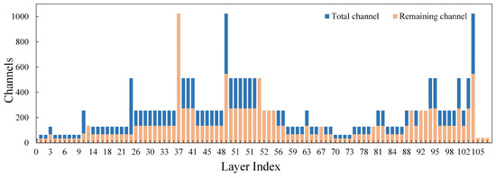
Figure 15.
Changes in the channels in each layer of the improved model before and after pruning.
3.8. Comparison Experiments with Different Object Detection Models
Many object detection tasks have used detection methods based on the YOLO series [58,59,60]. Under the conditions of ensuring accuracy and being lightweight, the classification of varieties and defects of corn seeds during transportation helped improve the sorting speed and provided technical references for subsequent hardware development. This study evaluated seven object detection algorithms, including Faster R-CNN, YOLOv5-m, YOLOv5-s, YOLOv7, YOLOv7-tiny, YOLOv8 and YOLOv11, to validate the effectiveness of the proposed YOLO-SBWL method in detecting corn seeds. The results are shown in Table 7.
Table 7.
The results of corn seeds using different object detection algorithms.
The results revealed that the mAP value of the above seven algorithms were 88.4%, 91.28%, 89.59%, 94.62%, 89.44%, 95.07%, 93.13% and 97.21%, respectively; the inference times were 46.55, 13.26, 9.7, 16.87, 8.68, 15.4, 12.19 and 10.82 ms, respectively; and the number of the model parameters were 51.12, 20.88, 7.03, 36.52, 6.03, 25.84, 20.04 and 11.60 M, respectively. Based on an analysis of the results in Figure 16, YOLO-SBWL had the fastest convergence speed and highest detection accuracy for corn seeds compared with the other seven algorithms. YOLOv8 and YOLOv11 performed well in terms of the mAP but lacked in model stability. However, since the maximum frame rate of the camera was 65.2 fps, resulting in a frame period of 15.3 ms, the inference time of 11 ms left little room for the exposure time of the camera and other image processing. This could lead to intense competition for resources between devices and may increase the response time of the system. Therefore, finding the optimal balance between image quality and inference speed by adjusting camera parameters remains to be explored.
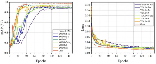
Figure 16.
mAP curves and the loss curves for seven object detection models.
The improved strategies of YOLO-SBWL demonstrate superior performance due to three key improvements. Firstly, the introduction of the SimAM enabled dynamic attention focusing on critical seed regions, enhancing the model’s ability to discern minute details during conveyor belt operations. Secondly, the BiFPN structure reinforced multi-scale information exchange, improving feature fusion capabilities for more precise differentiation between healthy seeds. Additionally, Wise-IoU accelerated the convergence speed while reducing loss values, further elevating the overall model performance. Although the model size was not the smallest, it achieved significant reduction from the baseline network while maintaining an optimal balance between accuracy and inference speed. In terms of resource consumption, pre-pruning models demonstrated GPU utilization between 70 and 86%, while post-pruning optimizations reduced this range to 45–76%. The final optimized model consumed only 1.2 GB of dedicated GPU memory; this demonstrated the effectiveness of our improvement strategy. In summary, YOLO-SBWL had a faster detection speed and the highest detection accuracy with the same dataset.
3.9. Comparative Experiments at Different Conveyor Speeds
As the conveyor belt speed increased, the corn seeds in the image became increasingly indistinct, as shown in Figure 17. This phenomenon occurred because elevated speeds caused the edges and texture details of the seeds to progressively blur. Specifically, the faster the speed, the greater the blur length became, while the direction of seed movement became discernible. High-speed conveyor belts were more prone to generating periodic vibrations, causing deviations in the seeds’ trajectories from ideal straight lines and introducing high-frequency noise. Therefore, in order to select the most suitable conveyor speed for this study, the detection results of the test models at different conveyor speeds were compared.
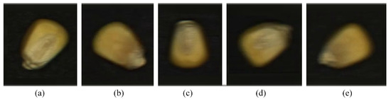
Figure 17.
Example diagram of corn seeds at five conveyor speeds: (a) 1000 rpm; (b) 2000 rpm; (c) 3000 rpm; (d) 4000 rpm; (e) 5000 rpm.
A moderate speed of 3000 rpm (0.195 m-s−1) was selected in consideration of the accuracy and efficiency required for the actual sorting process of corn seeds, as excessive speed would alter the positions of corn seeds, making precise localization difficult. The average accuracy of the model for corn seeds during the conveyor belt movement remained above 96.17%, and the inference times were within 11 ms (Table 8). The visualization results of the improved model were verified on the dynamic video image with a speed of 3000 rpm, as shown in Figure 18 and Video S1.
Table 8.
Detection results of corn seeds using the improved model at different conveyor speeds.
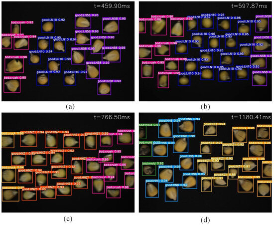
Figure 18.
Visualization results of proposed model on the dynamic video imagery at a speed of 3000 rpm (Video 1). (a) Frame 31, (b) Frame 40, (c) Frame 51 and (d) Frame 78.
4. Conclusions
The features of corn seeds in the images can become blurred during the transportation process because of the similar appearance of corn seeds. These problems can produce false detection, missed detection and low precision in identifying the varieties and defects of corn seeds. Herein, the proposed YOLO-SBWL method for identifying the varieties and defects of corn seeds was based on machine vision and an improved YOLOv7 network. It combined the SimAM module, BiFPN structure, Wise-IoU loss function and LAMP channel pruning method. YOLO-SBWL enhanced its learning ability and detection precision while effectively reducing computational complexity. The proposed YOLO-SBWL model achieved a mAP of 97.21%, which was 2.59% higher than the original network. The number of parameters in this model decreased by 68.09%, and the model size decreased by 67.21%. This demonstrated that the channel pruning method was an effective model compression strategy. The average accuracy of YOLO-SBWL for corn seeds during the conveyor belt movement remained above 96.17%, and the inference times were within 11 ms. In addition, YOLO-SBWL outperformed seven baseline networks, including Faster R-CNN, YOLOv5-m, YOLOv5s, YOLOv7, YOLOv7-tiny, YOLOv8 and YOLOv11, in terms of accuracy. The proposed method achieved the non-destructive and efficient real-time detection of varieties and defects in corn seeds. Future research will focus on integrating different external environments so that the model can adapt to more complex environments.
Although the YOLO-SBWL method proposed in this study demonstrated significant advantages in detecting corn seeds in real time, it still presented some limitations. Firstly, this study was conducted using a custom dataset for training and testing, where the seeds did not overlap or make contact. If applied to more complex conditions, such as densely packed seeds or occlusion, the improvement strategies proposed for addressing the recognition problem of the model may be affected. Under compact or occluded conditions, important features of damaged seeds may be obscured, leading to multiple prediction boxes during seed recognition and potentially impacting the prediction results of the model.
Secondly, the damaged seeds used in this experiment, such as those with mold or cracks, were all externally damaged. Detecting internal damage or potential changes in seeds may require spectral information beyond visible light, which is difficult to achieve with RGB imaging.
In terms of equipment, the experiments were conducted with fixed lighting and camera parameter settings, and the adjustable speed range of the conveyor belt was limited by the hardware itself. This limits our exploration of variable environmental conditions, such as changing the lighting scenario or increasing the operating speed, which deserve further investigation.
In the future, we plan to consider more potential environmental variables, such as varying lighting conditions and a wider range of seed types, to enhance the robustness and versatility of our model. We will also explore the use of spectral information in conjunction with deep learning for the study of internal seed damage and classification. Lastly, we will experiment with better model pruning algorithms to achieve a better balance between model performance and image quality, making it easier to deploy the model on embedded devices for real-time detection.
Supplementary Materials
The following supporting information can be downloaded at: https://www.mdpi.com/article/10.3390/agriculture15070685/s1, Video S1: The video of detecting corn seeds at 3000 rpm.
Author Contributions
Conceptualization, Y.C. and H.B.; methodology, Y.C.; software, Y.C. and X.G.; validation, Y.C. and Y.F.; formal analysis, H.B. and L.S.; investigation, X.G. and S.Y.; resources, L.S.; data curation, X.G. and S.Y.; writing—original draft preparation, Y.C.; writing—review and editing, Y.C. and H.B.; visualization, Y.C. and Y.F.; supervision, H.B. and Y.F.; project administration, H.B. and L.S.; funding acquisition, H.B. All authors have read and agreed to the published version of the manuscript.
Funding
This research was funded by the National Natural Science Foundation of China (62341503), Natural Science Foundation of Heilongjiang Province (PL2024F036), Key Research and Development Program of Heilongjiang (GZ20220121, 2022ZX03A06), University Nursing Program for Young Scholar with Creative Talents in Heilongjiang Province (UNPYSCT-2018012), and Fundamental Research Funds for the Heilongjiang Provincial Universities (2023-KYYWF-1453).
Institutional Review Board Statement
Not applicable.
Data Availability Statement
Data are contained within the article or Supplementary Materials. The original contributions presented in this study are included in the article/Supplementary Materials. Further inquiries can be directed to the corresponding author.
Conflicts of Interest
The authors declare no conflicts of interest.
References
- Dai, D.; Ma, Z.; Song, R. Maize kernel development. Mol. Breed. 2021, 41, 2. [Google Scholar] [CrossRef] [PubMed]
- Javanmardi, S.; Miraei Ashtiani, S.-H.; Verbeek, F.J.; Martynenko, A. Computer-vision classification of corn seed varieties using deep convolutional neural network. J. Stored Prod. Res. 2021, 92, 101800. [Google Scholar] [CrossRef]
- Yu, L.; Liu, W.; Li, W.; Qin, H.; Xu, J.; Zuo, M. Non-destructive identification of maize haploid seeds using nonlinear analysis method based on their near-infrared spectra. Biosyst. Eng. 2018, 172, 144–153. [Google Scholar] [CrossRef]
- Yang, G.; Wang, Q.; Liu, C.; Wang, X.; Fan, S.; Huang, W. Rapid and visual detection of the main chemical compositions in maize seeds based on Raman hyperspectral imaging. Spectrochim. Acta Part A Mol. Biomol. Spectrosc. 2018, 200, 186–194. [Google Scholar] [CrossRef]
- Wang, Y.; Peng, Y.; Qiao, X.; Zhuang, Q. Discriminant analysis and comparison of corn seed vigor based on multiband spectrum. Comput. Electron. Agric. 2021, 190, 106444. [Google Scholar] [CrossRef]
- Zhang, Y.; Lv, C.; Wang, D.; Mao, W.; Li, J. A novel image detection method for internal cracks in corn seeds in an industrial inspection line. Comput. Electron. Agric. 2022, 197, 106930. [Google Scholar] [CrossRef]
- Fan, S.; Li, J.; Zhang, Y.; Tian, X.; Wang, Q.; He, X.; Zhang, C.; Huang, W. On line detection of defective apples using computer vision system combined with deep learning methods. J. Food Eng. 2020, 286, 110102. [Google Scholar] [CrossRef]
- Yang, X.; Zhang, S.; Liu, J.; Gao, Q.; Dong, S.; Zhou, C. Deep learning for smart fish farming: Applications, opportunities and challenges. Rev. Aquac. 2020, 13, 66–90. [Google Scholar] [CrossRef]
- Wang, B.; Yin, J.; Liu, J.; Fang, H.; Li, J.; Sun, X.; Guo, Y.; Xia, L. Extraction and classification of apple defects under uneven illumination based on machine vision. J. Food Process. Eng. 2022, 45, e13976. [Google Scholar] [CrossRef]
- Xu, J.; Lu, Y.; Olaniyi, E.; Harvey, L.; Lu, R. Online volume measurement of sweetpotatoes by A LiDAR-based machine vision system. J. Food Eng. 2024, 361, 111725. [Google Scholar] [CrossRef]
- Guo, J.; Liang, J.; Xia, H.; Ma, C.; Lin, J.; Qiao, X. An Improved Inception Network to classify black tea appearance quality. J. Food Eng. 2024, 369, 111931. [Google Scholar] [CrossRef]
- Altuntaş, Y.; Cömert, Z.; Kocamaz, A.F. Identification of haploid and diploid maize seeds using convolutional neural networks and a transfer learning approach. Comput. Electron. Agric. 2019, 163, 104874. [Google Scholar] [CrossRef]
- Kurtulmuş, F. Identification of sunflower seeds with deep convolutional neural networks. J. Food Meas. Charact. 2021, 15, 1024–1033. [Google Scholar] [CrossRef]
- Zhou, Q.; Huang, W.; Tian, X.; Yang, Y.; Liang, D. Identification of the variety of maize seeds based on hyperspectral images coupled with convolutional neural networks and subregional voting. J. Sci. Food Agric. 2021, 101, 4532–4542. [Google Scholar] [CrossRef]
- Luo, T.; Zhao, J.; Gu, Y.; Zhang, S.; Qiao, X.; Tian, W.; Han, Y. Classification of weed seeds based on visual images and deep learning. Inf. Process. Agric. 2023, 10, 40–51. [Google Scholar] [CrossRef]
- Feng, Y.; Zhao, X.; Tian, R.; Liang, C.; Liu, J.; Fan, X. Research on an Intelligent Seed-Sorting Method and Sorter Based on Machine Vision and Lightweight YOLOv5n. Agronomy 2024, 14, 1953. [Google Scholar] [CrossRef]
- Peng, J.; Yang, Z.; Lv, D.; Yuan, Z. A dynamic rice seed counting algorithm based on stack elimination. Measurement 2024, 227, 114275. [Google Scholar] [CrossRef]
- Süme, S.; Ponomarjova, K.-M.; Wendt, T.M.; Rupitsch, S.J. Enhancing human–robot collaboration with thermal images and deep neural networks: The unique thermal industrial dataset WLRI-HRC and evaluation of convolutional neural networks. J. Sens. Sens. Syst. 2025, 14, 37–46. [Google Scholar] [CrossRef]
- Dananjayan, S.; Tang, Y.; Zhuang, J.; Hou, C.; Luo, S. Assessment of state-of-the-art deep learning based citrus disease detection techniques using annotated optical leaf images. Comput. Electron. Agric. 2022, 193, 106658. [Google Scholar] [CrossRef]
- Ouf, N.S. Leguminous seeds detection based on convolutional neural networks: Comparison of faster R-CNN and YOLOv4 on a small custom dataset. Artif. Intell. Agric. 2023, 8, 30–45. [Google Scholar] [CrossRef]
- Shi, Y.; Li, J.; Yu, Z.; Li, Y.; Hu, Y.; Wu, L. Multi-Barley Seed Detection Using iPhone Images and YOLOv5 Model. Foods 2022, 11, 3531. [Google Scholar] [CrossRef] [PubMed]
- Sundaramurthy, R.P.T.; Balasubramanian, Y.; Annamalai, M. Real-time detection of Fusarium infection in moving corn grains using YOLOv5 object detection algorithm. J. Food Process. Eng. 2023, 46, e14401. [Google Scholar] [CrossRef]
- Wan, F.; Sun, C.; He, H.; Lei, G.; Xu, L.; Xiao, T. YOLO-LRDD: A lightweight method for road damage detection based on improved YOLOv5s. EURASIP J. Adv. Signal Process. 2022, 2022, 98. [Google Scholar] [CrossRef]
- Zhou, S.; Cai, K.; Feng, Y.; Tang, X.; Pang, H.; He, J.; Shi, X. An Accurate Detection Model of Takifugu rubripes Using an Improved YOLO-V7 Network. J. Mar. Sci. Eng. 2023, 11, 1051. [Google Scholar] [CrossRef]
- Zhang, X.; Xuan, C.; Hou, Z. Recognition model for coated red clover seeds using YOLOv5s optimized with an attention module. Int. J. Agric. Biol. Eng. 2024, 16, 207–214. [Google Scholar] [CrossRef]
- Zhang, P.; Li, D. EPSA-YOLO-V5s: A novel method for detecting the survival rate of rapeseed in a plant factory based on multiple guarantee mechanisms. Comput. Electron. Agric. 2022, 193, 106714. [Google Scholar] [CrossRef]
- Zhao, J.; Xi, X.; Shi, Y.; Zhang, B.; Qu, J.; Zhang, Y.; Zhu, Z.; Zhang, R. An Online Method for Detecting Seeding Performance Based on Improved YOLOv5s Model. Agronomy 2023, 13, 2391. [Google Scholar] [CrossRef]
- Xiao, Z.; Sun, E.; Yuan, F.; Peng, J.; Liu, J. Detection Method of Damaged Camellia Oleifera Seeds Based on YOLOv5-CB. IEEE Access 2022, 10, 126133–126141. [Google Scholar] [CrossRef]
- Wang, Y.; Bai, H.; Sun, L.; Tang, Y.; Huo, Y.; Min, R. The Rapid and Accurate Detection of Kidney Bean Seeds Based on a Compressed Yolov3 Model. Agriculture 2022, 12, 1202. [Google Scholar] [CrossRef]
- Beyaz, A.; Saripinar, Z. Sugar Beet Seed Classification for Production Quality Improvement by Using YOLO and NVIDIA Artificial Intelligence Boards. Sugar Tech 2024, 26, 1751–1759. [Google Scholar] [CrossRef]
- Xia, Y.; Che, T.; Meng, J.; Hu, J.; Qiao, G.; Liu, W.; Kang, J.; Tang, W. Detection of surface defects for maize seeds based on YOLOv5. J. Stored Prod. Res. 2024, 105, 102242. [Google Scholar] [CrossRef]
- Jiao, Y.; Wang, Z.; Shang, Y.; Li, R.; Hua, Z.; Song, H. Detecting endosperm cracks in soaked maize using μCT technology and R-YOLOv7-tiny. Comput. Electron. Agric. 2023, 213, 108232. [Google Scholar] [CrossRef]
- Li, A.; Wang, C.; Ji, T.; Wang, Q.; Zhang, T. D3-YOLOv10: Improved YOLOv10-Based Lightweight Tomato Detection Algorithm Under Facility Scenario. Agriculture 2025, 14, 2268. [Google Scholar] [CrossRef]
- Abulizi, A.; Ye, J.; Abudukelimu, H.; Guo, W. DM-YOLO: Improved YOLOv9 model for tomato leaf disease detection. Front. Plant Sci. 2024, 15, 1473928. [Google Scholar] [CrossRef] [PubMed]
- Ali, M.L.; Zhang, Z. The YOLO Framework: A Comprehensive Review of Evolution, Applications, and Benchmarks in Object Detection. Computers 2024, 13, 336. [Google Scholar] [CrossRef]
- Jing, C.; Fu, T.; Li, F.; Jin, L.; Song, R. FPC-BTB detection and positioning system based on optimized YOLOv5. Biomim. Intell. Robot. 2023, 3, 100132. [Google Scholar] [CrossRef]
- Wang, J.; Shen, M.; Liu, L.; Xu, Y.; Okinda, C. Recognition and Classification of Broiler Droppings Based on Deep Convolutional Neural Network. J. Sens. 2019, 2019, 3823515. [Google Scholar] [CrossRef]
- Hong, S.; Jiang, Z.; Liu, L.; Wang, J.; Zhou, L.; Xu, J. Improved Mask R-CNN Combined with Otsu Preprocessing for Rice Panicle Detection and Segmentation. Appl. Sci. 2022, 12, 11701. [Google Scholar] [CrossRef]
- Felsch, M.; Meyer, O.; Schlickenrieder, A.; Engels, P.; Schönewolf, J.; Zöllner, F.; Heinrich-Weltzien, R.; Hesenius, M.; Hickel, R.; Gruhn, V.; et al. Detection and localization of caries and hypomineralization on dental photographs with a vision transformer model. npj Digit. Med. 2023, 6, 198. [Google Scholar] [CrossRef]
- Takaya, K.; Shibata, A.; Mizuno, Y.; Ise, T. Unmanned aerial vehicles and deep learning for assessment of anthropogenic marine debris on beaches on an island in a semi-enclosed sea in Japan. Environ. Res. Commun. 2022, 4, 015003. [Google Scholar] [CrossRef]
- Chen, L.; Wu, J.; Xie, Y.; Chen, E.; Zhang, X. Discriminative feature constraints via supervised contrastive learning for few-shot forest tree species classification using airborne hyperspectral images. Remote. Sens. Environ. 2023, 295, 113710. [Google Scholar] [CrossRef]
- Li, Z.; Zhu, Y.; Sui, S.; Zhao, Y.; Liu, P.; Li, X. Real-time detection and counting of wheat ears based on improved YOLOv7. Comput. Electron. Agric. 2024, 218, 108670. [Google Scholar] [CrossRef]
- Hu, J.; Shen, L.; Sun, G. Squeeze-and-excitation networks. In Proceedings of the IEEE Conference on Computer Vision and Pattern Recognition, Salt Lake City, UT, USA, 18–22 June 2018; pp. 7132–7141. [Google Scholar] [CrossRef]
- Woo, S.; Park, J.; Lee, J.Y.; Kweon, I.S. Cbam: Convolutional block attention module. In Proceedings of the European Conference on Computer Vision (ECCV), Munich, Germany, 8–14 September 2018; pp. 3–19. [Google Scholar]
- Yang, L.; Zhang, R.Y.; Li, L.; Xie, X. Simam: A simple, parameter-free attention module for convolutional neural networks. In Proceedings of the International Conference on Machine Learning (PMLR), Online, 18–24 July 2021; pp. 11863–11874. [Google Scholar]
- Liang, L.; Zhang, Y.; Zhang, S.; Li, J.; Plaza, A.; Kang, X. Fast Hyperspectral image classification combining transformers and SimAM-Based CNNs. IEEE Trans. Geosci. Remote Sens. 2023, 61, 5522219. [Google Scholar] [CrossRef]
- Dang, F.; Chen, D.; Lu, Y.; Li, Z. YOLOWeeds: A novel benchmark of YOLO object detectors for multi-class weed detection in cotton production systems. Comput. Electron. Agric. 2023, 205, 107655. [Google Scholar] [CrossRef]
- Tang, T.; Wang, X.; Ma, Z.; Hong, W.; Yu, G.; Ye, B. Lightweight detection method for lotus seedpod in natural environment. Int. J. Agric. Biol. Eng. 2024, 16, 197–206. [Google Scholar] [CrossRef]
- Wu, D.; Lv, S.; Jiang, M.; Song, H. Using channel pruning-based YOLO v4 deep learning algorithm for the real-time and accurate detection of apple flowers in natural environments. Comput. Electron. Agric. 2020, 178, 105742. [Google Scholar] [CrossRef]
- Wang, D.; He, D. Channel pruned YOLO V5s-based deep learning approach for rapid and accurate apple fruitlet detection before fruit thinning. Biosyst. Eng. 2021, 210, 271–281. [Google Scholar] [CrossRef]
- Lee, J.; Park, S.; Mo, S.; Ahn, S.; Shin, J. Layer-adaptive sparsity for the magnitude-based pruning. arXiv 2020, arXiv:2010.07611. [Google Scholar]
- Smith, L.N. Cyclical Learning Rates for Training Neural Networks. In Proceedings of the 2017 IEEE Winter Conference on Applications of Computer Vision (WACV), Santa Rosa, CA, USA, 24–31 March 2017; pp. 464–472. [Google Scholar] [CrossRef]
- Wang, C.-Y.; Bochkovskiy, A.; Liao, H.-Y.M. YOLOv7: Trainable bag-of-freebies sets new state-of-the-art for real-time object detectors. In Proceedings of the 2023 IEEE/CVF Conference on Computer Vision and Pattern Recognition (CVPR), Vancouver, BC, Canada, 17–24 June 2023; pp. 7464–7475. [Google Scholar] [CrossRef]
- Zoubek, T.; Bumbálek, R.; Ufitikirezi, J.d.D.M.; Strob, M.; Filip, M.; Špalek, F.; Heřmánek, A.; Bartoš, P. Advancing precision agriculture with computer vision: A comparative study of YOLO models for weed and crop recognition. Crop. Prot. 2025, 190, 107076. [Google Scholar] [CrossRef]
- Yang, H.; Liu, Y.; Wang, S.; Qu, H.; Li, N.; Wu, J.; Yan, Y.; Zhang, H.; Wang, J.; Qiu, J. Improved Apple Fruit Target Recognition Method Based on YOLOv7 Model. Agriculture 2023, 13, 1278. [Google Scholar] [CrossRef]
- Yuan, C.; Liu, T.; Gao, F.; Zhang, R.; Seng, X. YOLOv5s-CBAM-DMLHead: A lightweight identification algorithm for weedy rice (Oryza sativa f. spontanea) based on improved YOLOv5. Crop. Prot. 2023, 172, 106342. [Google Scholar] [CrossRef]
- Bai, Y.; Yu, J.; Yang, S.; Ning, J. An improved YOLO algorithm for detecting flowers and fruits on strawberry seedlings. Biosyst. Eng. 2024, 237, 1–12. [Google Scholar] [CrossRef]
- Tang, Y.; Zhou, H.; Wang, H.; Zhang, Y. Fruit detection and positioning technology for a Camellia oleifera C. Abel orchard based on improved YOLOv4-tiny model and binocular stereo vision. Expert Syst. Appl. 2023, 211, 118573. [Google Scholar] [CrossRef]
- Fan, S.; Liang, X.; Huang, W.; Zhang, V.J.; Pang, Q.; He, X.; Li, L.; Zhang, C. Real-time defects detection for apple sorting using NIR cameras with pruning-based YOLOV4 network. Comput. Electron. Agric. 2022, 193, 106715. [Google Scholar] [CrossRef]
- Zhao, J.; Ma, Y.; Yong, K.; Zhu, M.; Wang, Y.; Luo, Z.; Wei, X.; Huang, X. Deep-learning-based automatic evaluation of rice seed germination rate. J. Sci. Food Agric. 2023, 103, 1912–1924. [Google Scholar] [CrossRef]
Disclaimer/Publisher’s Note: The statements, opinions and data contained in all publications are solely those of the individual author(s) and contributor(s) and not of MDPI and/or the editor(s). MDPI and/or the editor(s) disclaim responsibility for any injury to people or property resulting from any ideas, methods, instructions or products referred to in the content. |
© 2025 by the authors. Licensee MDPI, Basel, Switzerland. This article is an open access article distributed under the terms and conditions of the Creative Commons Attribution (CC BY) license (https://creativecommons.org/licenses/by/4.0/).