A Variable-Threshold Segmentation Method for Rice Row Detection Considering Robot Travelling Prior Information

Abstract

Accurate rice row detection is critical for autonomous agricultural machinery navigation in complex paddy environments. Existing methods struggle with terrain unevenness, water reflections, and weed interference. This study aimed to develop a robust rice row detection method by integrating multi-sensor data and leveraging robot travelling prior information. A 3D point cloud acquisition system combining 2D LiDAR, AHRS, and RTK-GNSS was designed. A variable-threshold segmentation method, dynamically adjusted based on real-time posture perception, was proposed to handle terrain variations. Additionally, a clustering algorithm incorporating rice row spacing and robot path constraints was developed to filter noise and classify seedlings. Experiments in dryland with simulated seedlings and real paddy fields demonstrated high accuracy: maximum absolute errors of 59.41 mm (dryland) and 69.36 mm (paddy), with standard deviations of 14.79 mm and 19.18 mm, respectively. The method achieved a 0.6489° mean angular error, outperforming existing algorithms. The fusion of posture-aware thresholding and path-based clustering effectively addresses the challenges in complex rice fields. This work enhances the automation of field management, offering a reliable solution for precision agriculture in unstructured environments. Its technical framework can be adapted to other row crop systems, promoting sustainable mechanization in global rice production.

1. Introduction

Rice is one of the three most important staple crops worldwide, predominantly grown in the Asian monsoon region. In addition to its significant water requirements, which make efficient water management crucial for sustainable production [1,2], rice cultivation also plays a vital role in rural livelihoods, economic stability, and cultural practices, particularly in the Asian monsoon region [3]. However, rice production still involves numerous processes and remains labor-intensive. During the mid-term management phase of paddy fields (including operations such as weeding, fertilization, and pesticide application), the mechanization level remains notably low at merely 16.84% [4]. The primary machinery used for tasks such as fertilization and pest control in rice fields is the highland gap sprayer, which requires the operator to remain vigilant to prevent the tires from damaging the rice plants. Similarly, rice weeding machines must also be operated carefully to avoid crushing the rice crops. Therefore, in complex agricultural environments, the rapid and accurate identification of rice rows is crucial in enhancing the automation of field management. This rice row recognition is essential in achieving automatic tracking and control in agricultural machinery.

Currently, both domestic and international scholars primarily focus on crop row recognition using ultrasonic sensors, visual sensors, and LiDAR. Ultrasonic waves exhibit significant energy attenuation during atmospheric propagation, accompanied by lower ranging accuracy and limited directivity. Additionally, their performance is susceptible to temperature variations. These inherent limitations make ultrasonic technology generally unsuitable as a standalone solution for environmental perception applications requiring high precision [5]. However, it remains applicable in scenarios with relaxed accuracy requirements, such as obstacle detection in parking assistance systems [6]. Visual sensors, while providing abundant information, face challenges due to the uncontrollable nature of agricultural environments, such as fluctuations in light intensity [7]. Despite the development of various algorithms to interpret environmental information, the results vary significantly depending on the environment, crop type, sensor choice, and algorithm used [8,9,10,11,12,13]. LiDAR has emerged as a prominent technology in precision agriculture (PA) due to its high ranging accuracy, excellent real-time performance, and strong anti-interference capabilities [14,15,16,17,18,19,20,21]. LiDAR systems are typically classified as either two-dimensional (2D) or three-dimensional (3D), based on their scanning mechanisms. While 3D LiDAR systems are expensive, 2D LiDAR systems offer simpler structures, faster detection speeds, and lower costs, making them more commonly used in research [22,23,24,25].

In complex agricultural environments, uneven terrain can cause significant bumps during vehicle movement. However, 2D LiDAR, lacking height information, struggles to fully reconstruct the terrain and may suffer from data distortion or false readings. To address this challenge, many researchers have incorporated additional sensors for posture correction, enabling the generation of 3D point cloud maps of crops. For example, Colaço et al. combined 2D LiDAR and GNSS to create a scanning system capable of generating 3D models of citrus trees, including the canopy volume and height [26]. Miguel Garrido et al. installed a total station, IMU, and multiple 2D LiDAR sensors oriented in different directions on a vehicle. Due to the limitations of single-directional LiDAR for crop detection, they employed the ICP algorithm to fuse point cloud data from different directions, thereby enhancing the accuracy and reliability of the resulting 3D point clouds [27]. Similarly, David et al. fused data from a total station, IMU, and 2D LiDAR sensors to generate 3D point clouds for the clustering of individual maize seedlings at various growth stages. In semi-structured environments, their crop detection system achieved a 100% detection rate. However, their approach did not account for the crop shape and struggled to filter out noise from weeds and other obstacles [28].

The paddy field environment in Southern China is highly complex, characterized by varying water and soil depths across different fields [29]. The presence of water layers in paddy fields presents significant challenges for visual identification systems through two primary mechanisms: (1) specular reflections from water surfaces [30] and (2) the chromatic and morphological characteristics of weeds, which closely resemble those of rice seedlings. These coexisting factors substantially compromise the reliability of computer vision-based weed detection in submerged agricultural environments. Additionally, the uneven hard bottom layer of paddy fields causes frequent posture changes in field operation machinery [31]. When a 2D LiDAR is mounted on a mobile platform, the reconstructed environmental data often suffer from inaccuracies in height information. To address these challenges, this study presents a 3D information acquisition system that integrates 2D LiDAR, an attitude and heading reference system (AHRS), and a global navigation satellite system (GNSS). Furthermore, a variable-threshold segmentation method is proposed, along with a rice row classification technique based on prior information.

2. Materials and Methods

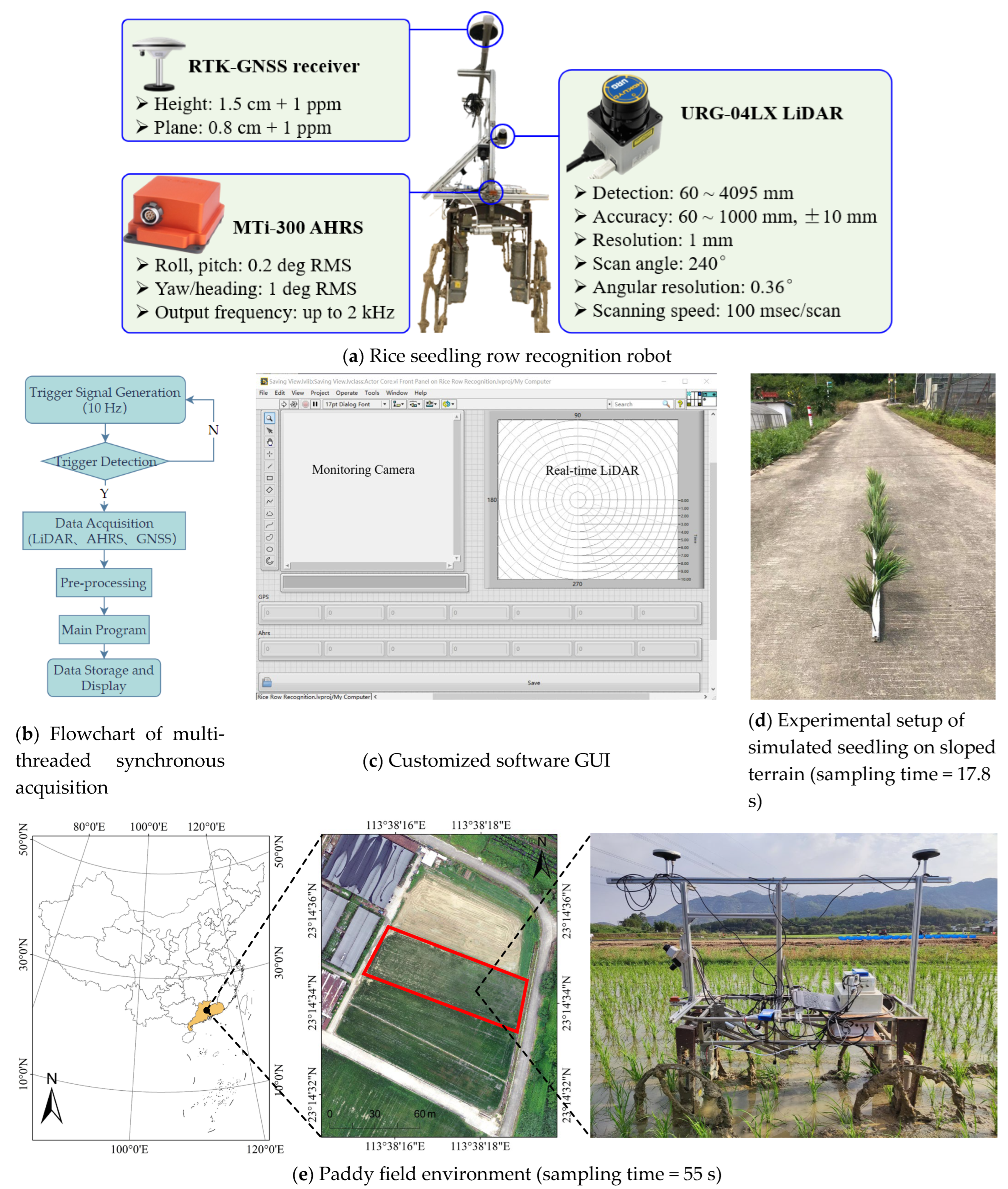
2.1. Three-Dimensional Point Cloud Acquisition and Preprocessing

2.1.1. LiDAR and AHRS Sensor Coordinate Calibration

Coordinate calibration, as illustrated in Figure 1, involves three coordinate systems: the LiDAR coordinate system ($O_l{X}_l{Y}_l{Z}_l$), the vehicle coordinate system ($O_V{X}_V{Y}_V{Z}_V$), and the geodetic coordinate system ($O_W{X}_W{Y}_W{Z}_W$). In this system, the $X_W$ and $Y_W$ coordinates are derived from the Gaussian–Krüger projection transformation within the WGS-84 geocentric coordinate system, while the $Z_W$ coordinate represents elevation information (the elevation is adjusted by subtracting the installation height).

Assuming that the robot is a rigid body, the vehicle coordinate system is defined with the point projected by the main GNSS antenna onto the ground as the origin ($O_V$).

(1)

Conversion of LiDAR Coordinate System to Vehicle Coordinate System

Assume that a LiDAR scanning point $P\left(\rho ,\theta \right)$ corresponds to the point $P_l=\left[\mathit{cos}\theta \ast \rho ; \mathit{sin}\theta \ast \rho ; 0\right]$ in the LiDAR coordinate system and the point $P_V=\left[X_V;Y_V;Z_V\right]$ in the vehicle coordinate system. Let the origin of the LiDAR coordinate system, denoted by $O_l$, be projected onto the vehicle coordinate system at $O_l^{\prime }$, while $O_v$ is the origin of the vehicle coordinate system. Therefore, the transformation from the LiDAR coordinate system to the vehicle coordinate system can be described as

$$P_V=\left[\begin{array}{ccc}1& 0& 0\\ 0& \mathit{cos}\phi & \mathit{sin}\phi \\ 0& -\mathit{sin}\phi & \mathit{cos}\phi \end{array}\right]\ast \left[\begin{array}{ccc}\mathit{cos}\left(-a\right)& 0& -\mathit{sin}\left(-a\right)\\ 0& 1& 0\\ \mathit{sin}\left(-a\right)& 0& \mathit{cos}\left(-a\right)\end{array}\right]\ast P_l+{\left[d_{x23};d_{y23};H_l\right]}^T$$

(1)

where $d_{x23}$ and $d_{y23}$ are the installation distances of $O_l^{\prime }$ and $O_v$ in the $X_V$ axis and $Y_V$ axis directions, respectively, in mm; $\alpha$ is the angle between the LiDAR and the vertical line ($Z_V$), in deg; $\phi$ is the angle between the LiDAR and the horizontal line ($Y_V$), in deg.

(2)

Conversion of the Vehicle Coordinate System to the Geodetic Coordinate System

The attitude and heading reference system (AHRS) is installed at the center of the front section of the vehicle to accurately measure the vehicle’s roll ($a_{-}x$) and pitch ($a_{-}y$) angles. The dual-antenna GNSS system provides the heading angle ($a_{-}z$). The comprehensive rotation matrix ^WR_V, which transforms the vehicle coordinate system to the geodetic coordinate system, can be derived from the global roll–pitch–heading (RPH) matrix (Equation (2)). Assuming that the origin of the vehicle coordinate system,$O_V$, corresponds to the point $O_{W_{-}V}$ in the geodetic coordinate system, and $O_{W_{-}G}$ denotes the current position as determined by the GNSS, the relationship between $O_{W_{-}V}$ and $O_{W_{-}G}$ is as shown in Equation (3).

$$\begin{gathered} {}_{ }{}^{W}R_V^{ }=R_Z^T\ast R_Y^T\ast R_X^T \\ =\left[\begin{array}{ccc}\mathit{cos}a\_y\mathit{cos}a\_z& -\mathit{cos}a\_x\mathit{sin}a\_z+\mathit{cos}a\_z\mathit{sin}a\_x\mathit{sin}a\_y& \mathit{sin}a\_x\mathit{sin}a\_z+\mathit{cos}a\_x\mathit{cos}a\_z\mathit{sin}a\_y\\ \mathit{cos}a\_y\mathit{sin}a\_z& \mathit{cos}a\_x\mathit{cos}a\_z+\mathit{sin}a\_x\mathit{sin}a\_y\mathit{sin}a\_z& -\mathit{sin}a\_x\mathit{cos}a\_z+\mathit{cos}a\_x\mathit{sin}a\_y\mathit{sin}a\_z\\ -\mathit{sin}a\_y& \mathit{cos}a\_y\mathit{sin}a\_x& \mathit{cos}a\_x\mathit{cos}a\_y\end{array}\right] \end{gathered}$$

(2)

$$O_{W_{-}V}=O_{W_{-}G}+{}_{ }{}^{W}R_V^{ }\ast \left(O_V-O_G\right)$$

(3)

As shown in Equation (4), the point in the vehicle coordinate system is transformed to the corresponding point in the geodetic coordinate system.

$$\left[\begin{array}{l}{X}_W\\ Y_W\\ Z_W\end{array}\right]=\left[\begin{array}{l}{X}_V\\ Y_V\\ Z_V\end{array}\right]\ast {}_{ }{}^{W}R_V^{ }+O_{W_{-}V}$$

(4)

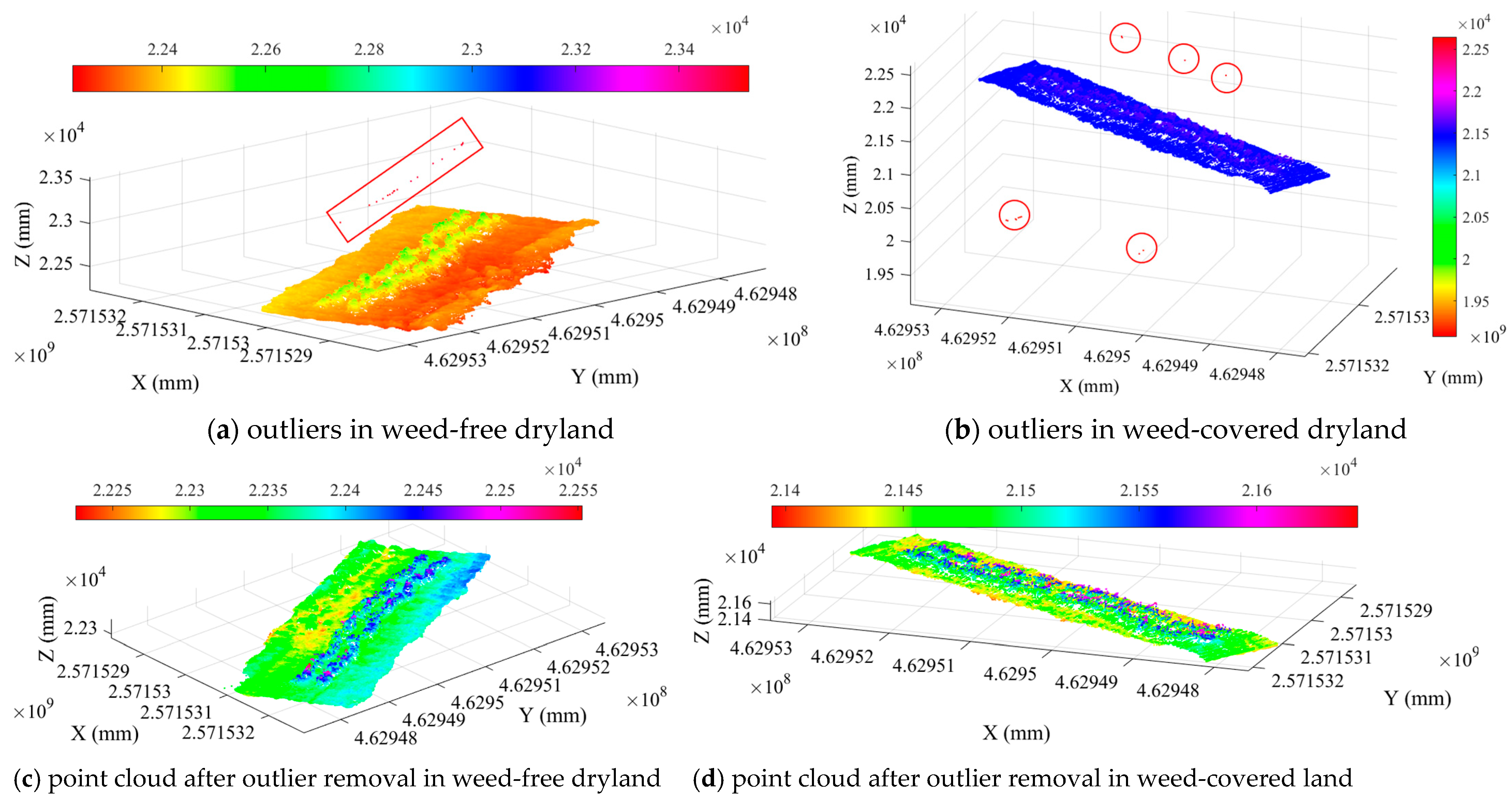
2.1.2. Outlier Elimination Based on the Pauta Criterion

The teleoperated robotic vehicle was navigated through uneven, weed-free, and weed-covered dryland (where simulated rice seedlings were pre-planted with 300 mm row spacing) to conduct sensor data pre-collection for algorithm development and parameter calibration, as illustrated in Figure 2.

Sharp edges and reflective surfaces can cause the misalignment of the LiDAR beam, resulting in “ghost points” [32], also known as outliers. As illustrated in Figure 3, the LiDAR data are converted from polar to Cartesian coordinates, which may introduce rough spots. These points typically deviate along the $X_l$-axis direction. To eliminate the influence of outliers, the Pauta criterion (also known as the 3σ criterion) is employed for detection and judgment.

The 3D point cloud data are reconstructed by fusing information from the LiDAR, AHRS, and GNSS sensors. Figure 4a,b display the 3D point cloud, including outliers (in red box and circles). The presence of outliers reduces the clarity of the environmental information. Figure 4c,d presents the 3D point cloud after outlier removal using the Pauta criterion, where different colors of solid points correspond to the varying height values of objects within the environment. The results demonstrate that the rice rows and ground features are clearly discernible, and the proposed method effectively mitigates the influence of outliers.

2.2. Rice Row Recognition Method Based on Multi-Sensor Information

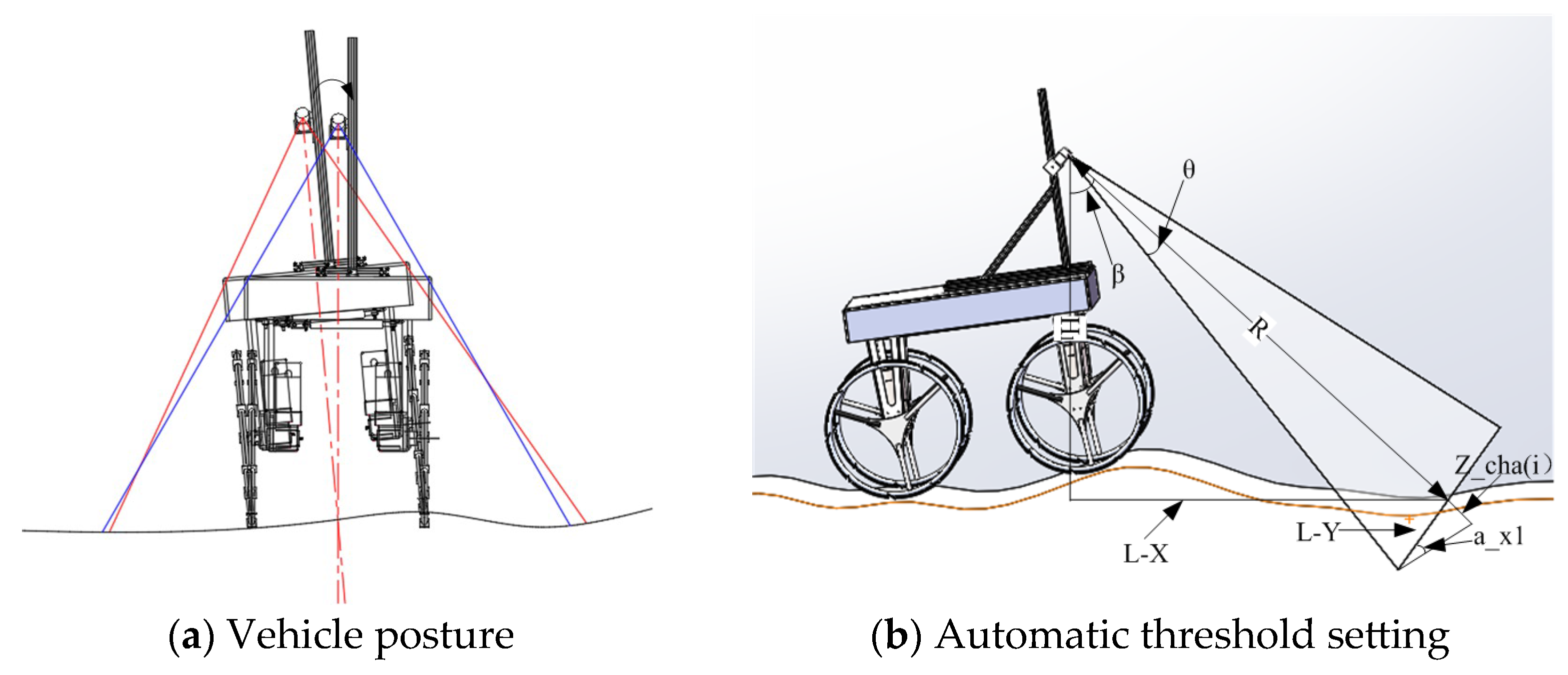
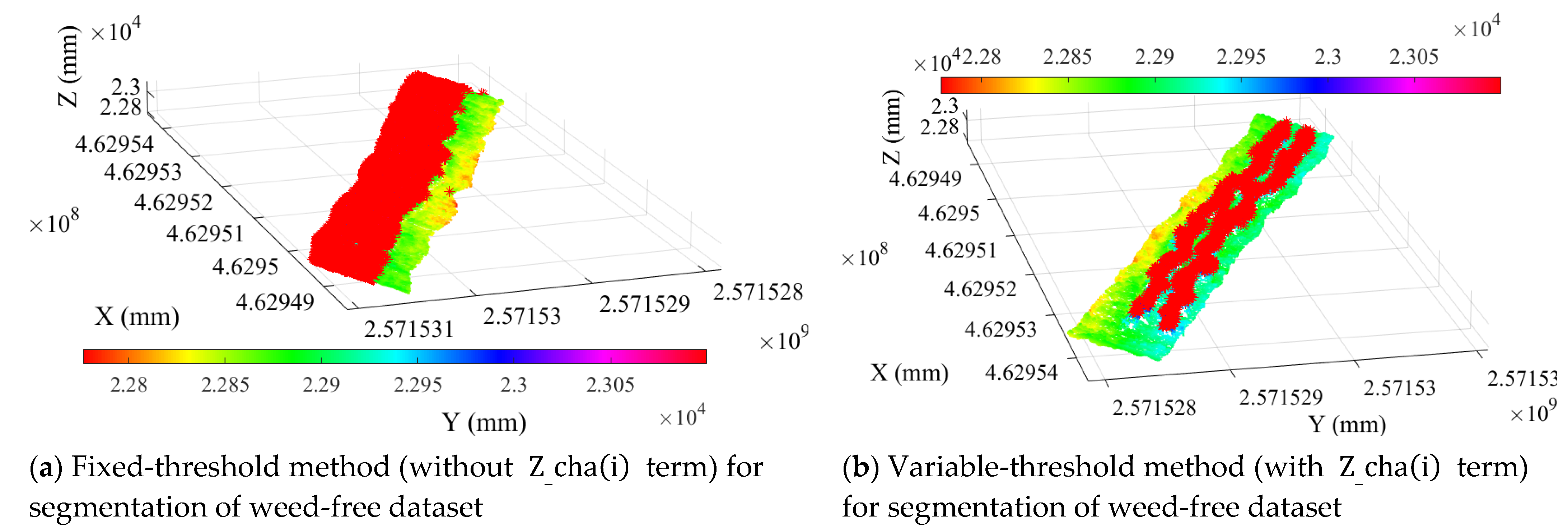
2.2.1. Variable-Threshold Object Segmentation Method Based on Posture Perception

Accurate object segmentation is a critical prerequisite for obstacle segmentation and recognition. Commonly employed object segmentation methods, such as plane fitting [33,34,35], often rely on simplifying assumptions about the environment. However, point cloud data, after outlier removal, more accurately reflect real field conditions. The height variations of individual data points are influenced by several factors, including the terrain and environmental conditions, which complicates the establishment of a fixed threshold for segmentation. To address this challenge, we propose a variable-threshold object segmentation method based on posture perception. This approach adapts the segmentation threshold dynamically, accommodating the variability in the field conditions and improving the segmentation accuracy.

As shown in Figure 5, due to the uneven hard layer of the paddy field, the robot’s posture undergoes frequent changes. Equation (5) is employed to correct the robot’s posture and mitigate the impact of posture variations on object segmentation. Using trigonometric relationships, the distance between the i-th LiDAR scanning line and the robot’s position can be calculated as $L_{-}X=H_l\ast \mathit{tan}\beta$, where $\beta =90°-\alpha$. Within the same LIDAR frame, the maximum height difference between the ground point cloud and the LiDAR scanning center point is given by

$$Z_{\_}cha\left(i\right)=L_{-}Y\ast tan\left(a_{-}x1\right)$$

(5)

where $L_{-}Y=abs\left(\mathit{tan}\theta \ast {\displaystyle \frac{H_l}{\mathit{cos}\beta }}\right)$, and θ represents the LiDAR’s field of view angle, while $a_{-}x1$ is the roll angle of the LiDAR scanning position. A certain distance exists between the current measured roll angle position of the robot and $a_{-}x1$.

In general, the closer the LiDAR frame is to the LiDAR scanning line, the smaller the corresponding roll angle error. Based on this observation, we propose using an exponential smoothing model for data prediction. The exponential smoothing model is an enhanced version of the moving average model, with the key feature that the weight of the data increases as the data points grow closer in time, with the most recent data receiving the highest weight. Therefore, the exponential smoothing model is chosen for data prediction [36]. The smoothing equation is expressed as

$$a_{-}x1=k_a\ast a_{-}x\left(i\right)+k_a\ast \left(1-k_a\right)\ast a_{-}x\left(i-1\right)+\cdots k_a\ast {\left(1-k_a\right)}^9\ast a_{-}x\left(i-9\right)$$

(6)

where $K_a$ is the smoothing coefficient (with 0 < $K_a$ < 1). In the exponential smoothing model, the smoothing coefficient α directly determines the trade-off between prediction sensitivity and stability. According to [37,38], when handling time series with significant fluctuations, moderate smoothing (α = 0.3–0.5) is generally recommended to balance noise suppression and trend responsiveness. Considering the large fluctuations in the data, $K_a$ is set to 0.5.

If the value of $a_{-}x1$ is close to zero, it indicates that the ground is nearly flat. Conversely, if the value is significant, it suggests that the ground is uneven and there is a height difference within the LiDAR frame scanning area. By using trigonometric relationships to calculate the maximum possible height difference, the threshold $Z_{-}\mathrm{T}\left(i\right)$ is determined as in Equation (7):

$$Z_{-}\mathrm{T}\left(i\right)=mean\left(Z_w\left(i,:\right)\right)+Z_{\_}cha\left(i\right)$$

(7)

where $Z_w\left(i,:\right)$ represents the height data of the ground point cloud, in mm.

To further validate the advantages of the proposed variable-threshold segmentation method, a set of comparative experiments was designed to evaluate its performance against conventional fixed-threshold segmentation, with the results presented in Figure 6. A comparative analysis of Figure 6a,b reveals that, while the fixed-threshold algorithm demonstrates limited efficacy in terrain segmentation by failing to completely isolate rice seedlings from the background, the proposed variable-threshold segmentation method successfully extracts two distinct rice seedling rows in the weed-free dryland. Equation (7) can only classify ground and non-ground point clouds, and it fails to segment seedlings from weeds in the weed-covered field (Figure 7a). To address this limitation, Equation (7) was enhanced by integrating the height differential between weeds and seedlings (where weeds exhibit lower vertical profiles than seedlings), yielding Equation (8) for complete seedling segmentation. The segmentation performance of Equation (8) in weed-covered scenarios is demonstrated in Figure 7b.

$$Z_{-}\mathrm{T}\left(i\right)=mean\left(Z_w\left(i,:\right)\right)+Z_{\_}cha\left(i\right)+PTh$$

(8)

where PTh represents the pass-through filter coefficient. Considering the emergence height of rice seedlings, the PTh value should satisfy PTh ≤ 40 for directly seeded fields and PTh ≤ 140 for transplanted fields. In this study, PTh is set to 30.

2.2.2. Rice Row Cluster Method Based on Prior Information

(1)

Extraction of the Center Point of Rice Rows

In a given LiDAR frame, there are significant positional differences between rice rows in the geodetic coordinate system. Based on this characteristic, the non-ground point cloud data for each LiDAR frame are classified to extract the center point. The specific steps are as follows.

• Threshold Setting

The threshold $T_{lidar}$ is determined based on the mathematical model derived in Equation (9). In this equation, the LiDAR’s angular resolution is 0.36° (HOKUYO’s URG-04LX), $line\_space$ represents the row spacing of the rice rows, and $w_{-}l\in \left[0,1\right]$ is the proportional coefficient. The row spacing parameter (line_space) can be dynamically set to 25 or 30 cm depending on the seeder type, while incorporating a row spacing variation coefficient w_l to quantify field-level fluctuations caused by mechanical vibrations and terrain undulations.

$$T_{lidar}={\displaystyle \frac{line\_space\ast w\_l}{L\_Y}}\ast {\displaystyle \frac{abs\left(\theta \right)}{0.36}}={\displaystyle \frac{line\_space\ast w\_l}{abs\left(tan\theta \ast \frac{H_L}{\mathit{cos}\beta }\right)}}\ast {\displaystyle \frac{abs\left(\theta \right)}{0.36}}$$

(9)

• Data Classification

The non-ground point cloud data are classified by calculating their spatial characteristics and comparing them with the threshold $T_{lidar}$. This results in the classification of the data points into distinct groups.

• Center Point Extraction

If the classified point cloud data contain multiple rice rows, the center point of each cluster is identified by extracting the midpoint within each category.

If only one category is identified, the midpoint of the entire non-ground point cloud data is set as the center point.

(2)

Center Point Classification Based on Robot Travelling Path

In seedling row recognition, positional relationships are commonly utilized for clustering [11]. As shown in Figure 8, the red dots represent the non-ground point data that have been denoised and processed to extract the center points from the LiDAR data, while the yellow route represents the robot’s travelling path, which separates two rows of rice. Additionally, the autonomous robot is equipped with a GNSS system. Based on this setup, a classification method is proposed that leverages the relationship between the rice rows and the robot’s travelling path (prior information).

• Horizontal Distance Calculation

First, in the same frame, the horizontal distance in the vehicle coordinate system between the center point of the rice row and the robot’s travelling path is computed. This distance is denoted as $dis$. In this study, the origin of the vehicle coordinate system is defined as the point where the main GNSS antenna projects onto the ground. Therefore, the robot’s travelling path serves as the origin of the vehicle coordinate system at different data acquisition times. If a point in the vehicle coordinate system is represented by $\left(X_V,Y_V,Z_V\right)$, the distance is given by

$$dis=Y_V$$

(10)

• Point Clustering

Next, the center points are clustered using Equation (11). Here, $line\_space$ denotes the rice row spacing, and $label$ is the variable representing the category label. Simultaneously, the variable $labe{l}_{-}nu{m}_{-}sum$ is used to count the number of center points in each category.

$$label=ceil\left({\displaystyle \frac{dis-line\_space\ast 0.5}{line\_space}}\right)$$

(11)

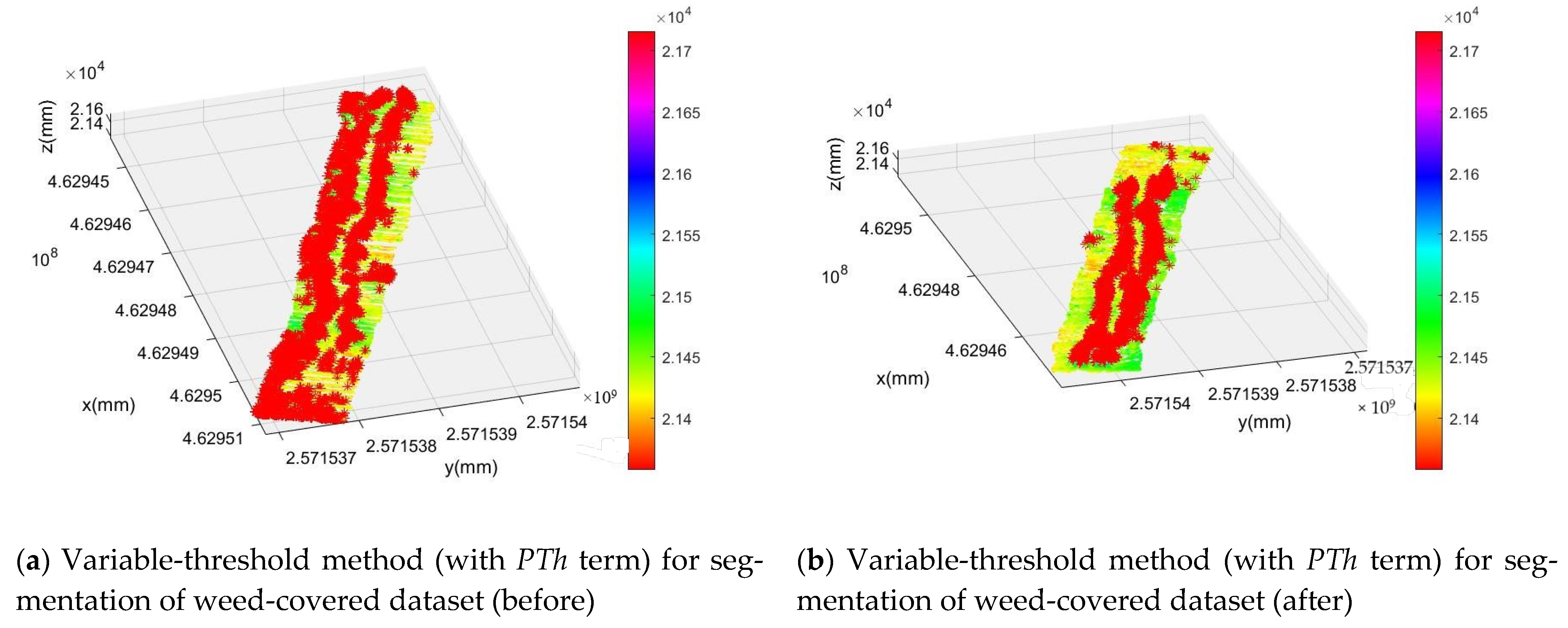
• Elimination of Small Weed Interference

While the point cloud data have already been processed to remove outliers and low weeds, some weeds that are comparable in height to rice may still remain. To further enhance the accuracy of rice row recognition, a second round of denoising is performed before fitting the rice rows. Given that rice is planted in rows, the number of center points within each clustering category is significantly greater than that of small-weed areas. A threshold value $T_{number}=mean\left(labe{l}_{-}nu{m}_{-}sum\right)$ is set. When the number of points within a cluster exceeds this threshold, the region is classified as a rice row. Otherwise, the area is considered noisy and is removed. Finally, as shown in Figure 9, the data corresponding to the $X_w$ and $Y_w$ axes of the seedling cluster are extracted.

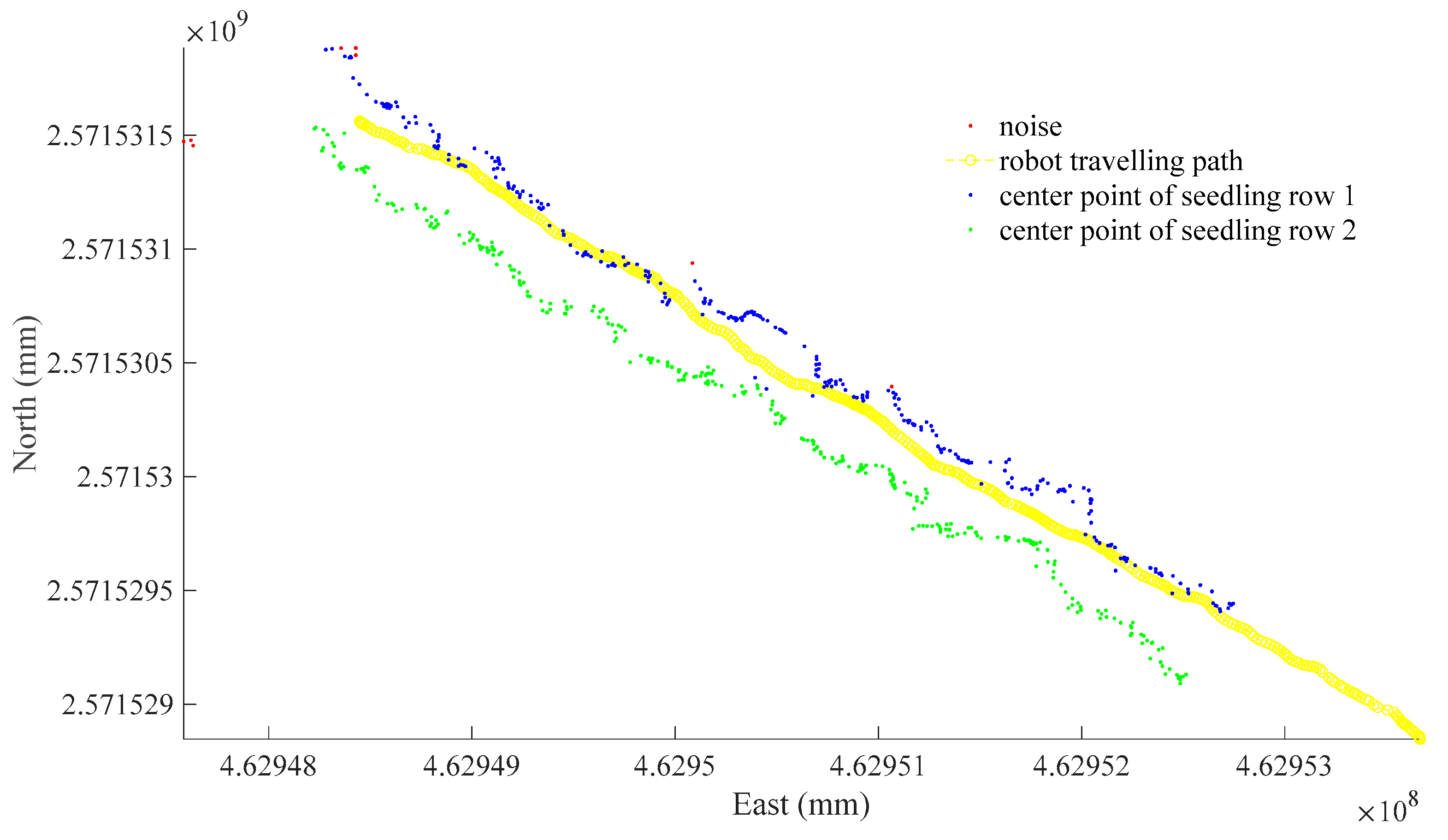
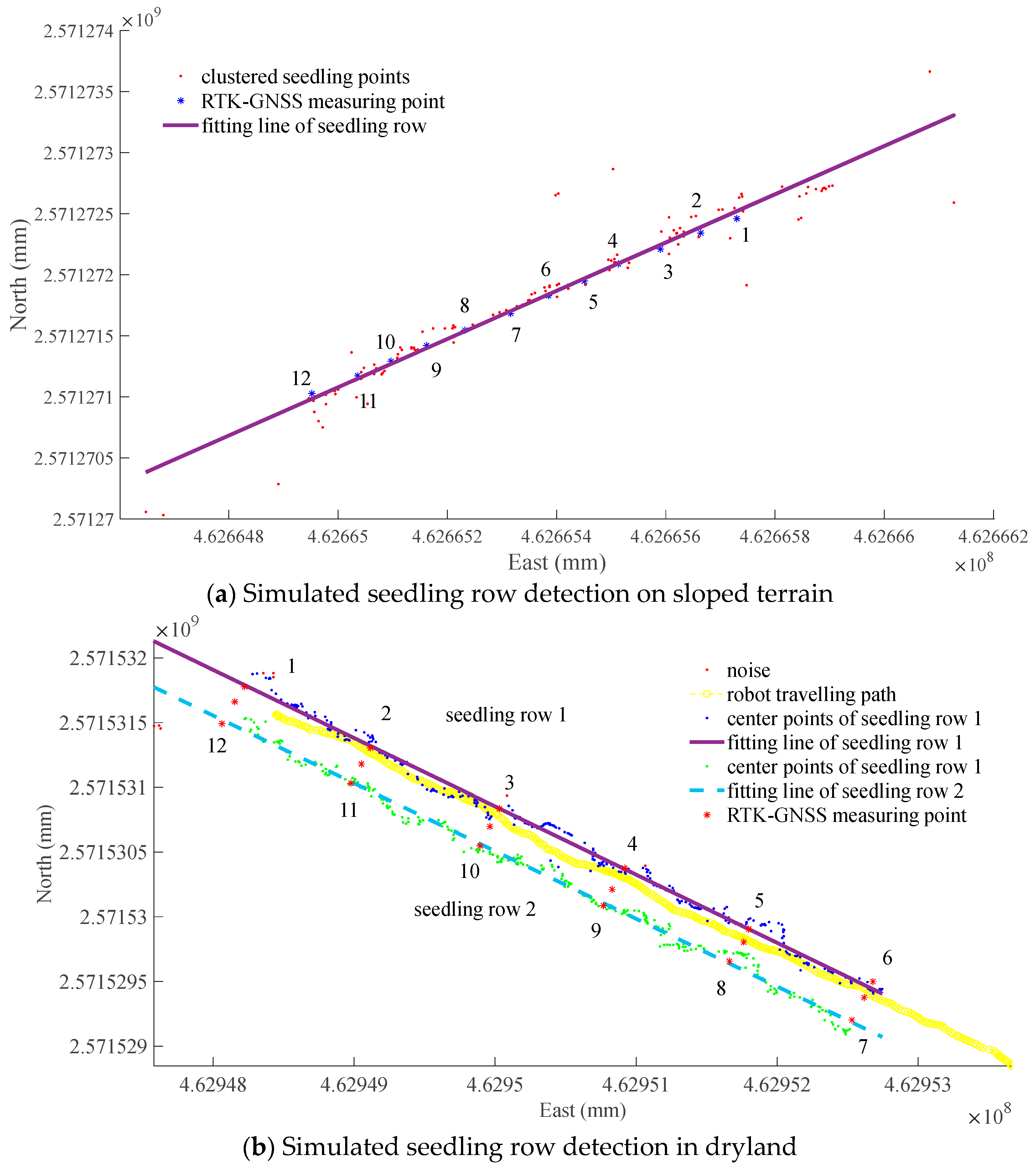
3. Experiment and Discussion

In order to verify the effectiveness of the algorithm, we used the robot to conduct validation experiments on sloped terrain (Figure 10d), in dryland (Figure 3a), and in a paddy field (Figure 10e). The experimental platform and environment are shown in Figure 10a. The data collection was composed of HOKUYO’s URG-04LX 2D LiDAR (10 Hz, ambient light resistance: 10,000 Lx or less), XSENS’ MTI-300 AHRS (10 Hz), and RTK-GNSS (10 Hz), etc. The sensor data acquisition system was i processed in the multithreaded software platform developed in LabVIEW 2015 (National Instruments, Austin, TX, USA. As shown in Figure 10b, a customized software architecture was specifically designed to handle parallel data processing from multiple sensor channels. The development environment operated on a Windows-based laptop (Core i5-7200U, 8GB DDR4 RAM), which provided sufficient computational resources for real-time data acquisition and processing tasks. The installation height of the 2D LiDAR was 1220 mm, with the angle α between the installation angle and $Z_v$ axis being 54.5°, and the angle φ between the installation angle and Y_v axis was 1.744°. The field of view angle was $\theta \in \left[-{10}^o,{12}^o\right]$, the installation height was $H_l=1220 \mathrm{mm}$, the proportional coefficient $w_{-}l=0.75$, and the rice planting row spacing was 300 mm. According to Equation (9), the clustering threshold was $T_{lidar}\approx \left[23.54,23.65\right]$. Therefore, in the experiment, the value of $T_{lidar}$ was set to 24.

During the experiment, the data collection platform moved in a straight line along the rice rows. The forward speeds of the experimental platform in the simulated and field environments were approximately 0.2 m/s and 1 m/s, respectively. The experimental site was located at the Zengcheng Experimental Base of South China Agricultural University in Guangzhou, China.

The rice row recognition results based on the robot’s travelling path are shown in Figure 11. In this figure, the yellow symbol represents the vehicle’s position in the geodetic coordinate system, obtained via the GNSS. The red asterisk (*) symbol indicates the manually measured position using the CTI RTK-DGPS I70. The solid points in various colors correspond to the center points of different objects: red points represent the center points of noisy areas, while blue and green points denote the center points of the rice rows. After clustering, the center points are fitted into straight lines using the robust regression method. Different line types represent the fitted results of different rice rows. The results indicate that the manually measured rice positions predominantly lie on the fitted straight lines of the rice rows.

In order to further evaluate the accuracy of the fitting rice line, the error ${\epsilon }_l$ was defined as the vertical distance from the RTK-GNSS measurement value to the fitting line. On the sloped terrain, the simulated seedling row fitting results were as shown in Figure 11a, where the linear equation for seedling rows is $y =1.9756\ast x+1657242002.64$. In the dryland, the simulated seedling row fitting results were as shown in Figure 11b, where the linear equations for seedling rows 1 and 2 are $y=-0.53\ast x+2817020373.78$ and $y=-0.524\ast x+2814010460.1$, respectively. In the paddy field, the fitting results of the seedling rows were as shown in Figure 11c. The linear equations for seedling rows 1 and 2 are $y=-0.3672\ast x+2741494099.49$ and $y=-0.3777\ast x+274637039.18$, respectively. The error analysis results of seedling position recognition are shown in

Table 1. Seedling position recognition results.

Seedling position recognition on sloped terrain	RTK-GNSS measuring point	1	2	3	4	5	6
	absolute error (mm)	27.42	21.82	15.86	1.81	9.72	5.03
	RTK-GNSS measuring point	7	8	9	10	11	12
	absolute error (mm)	9.40	4.12	9.67	9.86	10.09	19.55
Seedling position recognition in dryland	RTK-GNSS measuring point	1	2	3	4	5	6
	absolute error (mm)	15.18	14.70	0.86	10.57	4.89	59.41
	RTK-GNSS measuring point	7	8	9	10	11	12
	absolute error (mm)	27.04	10.87	13.31	16.59	16.41	16.09
Seedling position recognition in paddy field	RTK-GNSS measuring point	1	2	3	4	5	6
	absolute error (mm)	32.60	69.36	4.28	33.79	3.34	13.81
	RTK-GNSS measuring point	7	8	9	10	11	12
	absolute error (mm)	7.01	0.53	27.66	13.48	21.69	13.17

, where the maximum absolute error, minimum absolute error, and standard deviation on sloped terrain are shown to be 27.42 mm, 1.81 mm, and 7.66 mm, respectively; the maximum absolute error, minimum absolute error, and standard deviation in the dryland are 59.41 mm, 0.86 mm, and 14.79 mm, respectively; and the maximum error, minimum error, and standard deviation in the paddy field are 69.36 mm, 0.53 mm, and 19.18 mm, respectively.

The experimental results demonstrate that fusing data from LiDAR, AHRS, and GNSS enables the accurate reconstruction of 3D point cloud data. Furthermore, the straight lines fitted to the point cloud data effectively represent the positional information of the rice rows. The standard deviations under the two conditions are 14.79 mm and 19.18 mm, respectively. Notably, the position errors at point 6 in the simulated environment and at point 2 in the real environment are relatively large. The occurrence of significant errors can be attributed to the following factors. The objective of this study was to estimate the straight lines of seedling rows, thereby providing a reference path for robot navigation. Consequently, we employed a robust regression method to fit the positioning points of seedlings. The main characteristic of this method lies in its ability to identify and disregard potential points with a strong influence that deviate from the model structure, thereby ensuring the fitting effect of in-structure points. As a result, significant statistical errors may occur for individual outlier points (point 6 in the simulated environment and point 2 in the paddy field). For the task of robot navigation operations, it is beneficial to ignore individual outlier seedling points when fitting the straight line, as it aids in maintaining and controlling the stability of the heading. Therefore, future compensation is not necessary. Furthermore, the reference points used in this study correspond to the actual positions of the rice seedlings. However, due to variations in the soil’s bottom layer during the planting process, the precise positioning of seedlings—when transplanted or sown by machinery—inevitably deviates from the ideal straight-line path of the entire row. This inherent deviation can be attributed to the uneven nature of the field’s bottom layer, which affects the accurate alignment of the seedlings. To further evaluate the performance of the proposed algorithm, a comparative analysis was conducted against the crop row identification methods proposed in [38,39]. The quantitative comparison results are presented in

Table 2. Comparison of three algorithms for rice seedling centerline extraction.

Algorithm Type	Mean Angular Error (°)	Mean Processing Time (ms)
Proposed (paddy field)	0.6489	50.67
[38]	3.14	192.52
[39]	1.124	20.1

Note: The angular error metric is defined as the angle between the ground-truth line fitted to seedling positions and the estimated line derived by the proposed algorithm, ensuring consistent evaluation criteria with the referenced methods.

.

As evidenced in Table 2, the proposed algorithm achieves a significant improvement in angular accuracy, outperforming both [38] (by 79.3%) and [39] (by 42.3%). While the computational time of our method (50.67 ms per iteration) is moderately higher than that of [39], it successfully fulfills the real-time processing requirement for LiDAR data acquisition at 10 Hz. Furthermore, it should be noted that the current implementation leaves room for hardware optimization to enhance the computational efficiency.

4. Conclusions

This study presents a robust framework for rice row detection in complex paddy environments. Firstly, a multi-sensor fusion system integrating 2D LiDAR, AHRS, and RTK-GNSS was developed to reconstruct 3D point clouds, effectively compensating for height distortions caused by the uneven terrain. Secondly, the proposed variable-threshold segmentation method, dynamically adjusted through posture perception, demonstrated superior adaptability to field variations compared to fixed-threshold approaches. By incorporating robot travelling path constraints and prior information about the rice row spacing, the clustering algorithm successfully filtered out weed interference and achieved accurate seedling localization. Experimental validation across sloped land, dryland, and submerged paddy fields confirmed the method’s reliability, with standard deviations below 20 mm and angular errors under 0.65°, outperforming existing techniques. These results highlight the method’s potential to enhance the autonomous navigation accuracy in real-world agricultural operations. Future research will focus on optimizing the computational efficiency through hardware acceleration and integrating MEMS-IMU with stereo visual odometry to address GNSS-denied scenarios. Additionally, extending this framework to diverse crop types and multi-robot coordination systems will further advance precision agriculture technologies.

References

1. Dehghanpir, S.; Bazrafshan, O.; Nadi, S.; Jamshidi, S. Assessing the sustainability of Agricultural Water Use Based on Water Footprints of wheat and rice production. In Sustainability and Water Footprint; Springer: Cham, Switzerland, 2024; Volume 10, pp. 57–82. [Google Scholar]
2. Bwire, D.; Saito, H.; Sidle, R.C.; Nishiwaki, J. Water management and hydrological characteristics of paddy-rice fields under alternate wetting and drying irrigation practice as climate smart practice: A review. Agronomy 2024, 14, 1421. [Google Scholar] [CrossRef]
3. Zhang, L.; Zhang, F.; Zhang, K.; Liao, P.; Xu, Q. Effect of agricultural management practices on rice yield and greenhouse gas emissions in the rice–wheat rotation system in China. Sci. Total Environ. 2024, 916, 170307. [Google Scholar] [CrossRef]
4. Peng, S.; Zheng, C.; Yu, X. Progress and challenges of rice ratooning technology in China. Crop Environ. 2023, 2, 5–11. [Google Scholar] [CrossRef]
5. Chen, Q. China Agricultural Mechanization Yearbook; China Agricultural Science and Technology Press: Beijing, China, 2020. [Google Scholar]
6. He, Y.; Jiang, H.; Fang, H.; Wang, Y.; Liu, Y. Research progress of intelligent obstacle detection methods of vehicles and their application on agriculture. Trans. Chin. Soc. Agric. Eng. 2018, 34, 21–32. [Google Scholar]
7. Ji, Y.; Xu, H.; Zhang, M.; Li, S.; Cao, R.; Li, H. Design of Point Cloud Acquisition System for Farmland Environment Based on LiDAR. Trans. Chin. Soc. Agric. Mach. 2019, 50, 1–7. [Google Scholar]
8. Ji, C.; Zhou, J. Current Situation of Navigation Technologies for Agricultural Machinery. Trans. Chin. Soc. Agric. Mach. 2014, 45, 44–54. [Google Scholar]
9. Zhang, Q.; Chen, M.E.S.; Li, B. A visual navigation algorithm for paddy field weeding robot based on image understanding. Comput. Electron. Agric. 2017, 143, 66–78. [Google Scholar] [CrossRef]
10. Kaizu, Y.; Imou, K. A dual-spectral camera system for paddy rice seedling row detection. Comput. Electron. Agric. 2008, 63, 49–56. [Google Scholar] [CrossRef]
11. Zhang, X.; Li, X.; Zhang, B.; Zhou, J.; Tian, G.; Xiong, Y.; Gu, B. Automated robust crop-row detection in maize fields based on position clustering algorithm and shortest path method. Comput. Electron. Agric. 2018, 154, 165–175. [Google Scholar] [CrossRef]
12. Jing, G.; Yang, X.; Wang, Z.; Liu, H. Crop rows detection based on image characteristic point and particle swarm optimization-clustering algorithm. Trans. Chin. Soc. Agric. Eng. 2017, 33, 165–170. [Google Scholar]
13. Choi, K.H.; Han, S.K.; Han, S.H.; Park, K.H.; Kim, K.S.; Kim, S. Morphology-based guidance line extraction for an autonomous weeding robot in paddy fields. Comput. Electron. Agric. 2015, 113, 266–274. [Google Scholar] [CrossRef]
14. Wang, S.; Dai, X.; Xu, N.; Zhang, P. Overview on Environment Perception Technology for Unmanned Ground Vehicle. J. Chang. Univ. Sci. Technol. (Nat. Sci. Ed.) 2017, 40, 1–6. [Google Scholar]
15. Chateau, T.; Debain, C.; Collange, F.; Trassoudaine, L.; Alizon, J. Automatic guidance of agricultural vehicles using a laser sensor. Comput. Electron. Agric. 2000, 28, 243–257. [Google Scholar] [CrossRef]
16. Barawid, O.C., Jr.; Mizushima, A.; Ishii, K.; Noguchi, N. Development of an Autonomous Navigation System using a Two-dimensional Laser Scanner in an Orchard Application. Biosyst. Eng. 2007, 96, 139–149. [Google Scholar] [CrossRef]
17. Hiremath, S.A.; Van Der Heijden, G.W.; Van Evert, F.K.; Stein, A.; Ter Braak, C.J. Laser range finder model for autonomous navigation of a robot in a maize field using a particle filter. Comput. Electron. Agric. 2014, 100, 41–50. [Google Scholar] [CrossRef]
18. Zhang, Y.; Zhou, J. Laser radar based orchard trunk detection. J. China Agric. Univ. 2015, 20, 249–255. [Google Scholar]
19. Hämmerle, M.; Höfle, B. Effects of reduced terrestrial LiDAR point density on high-resolution grain crop surface models in precision agriculture. Sensors 2014, 14, 24212–24230. [Google Scholar] [CrossRef]
20. Keightley, K.E.; Bawden, G.W. 3D volumetric modeling of grapevine biomass using Tripod LiDAR. Comput. Electron. Agric. 2010, 74, 305–312. [Google Scholar] [CrossRef]
21. Xue, J.; Dong, S.; Fan, B. Detection of Obstacles Based on Information Fusion for Autonomous Agricultural Vehicles. Trans. Chin. Soc. Agric. Mach. 2018, 49, 36–41. [Google Scholar]
22. Peng, Y.; Qu, D.; Zhong, Y.; Xie, S.; Luo, J.; Gu, J. The obstacle detection and obstacle avoidance algorithm based on 2-D LiDAR. In Proceedings of the 2015 IEEE International Conference on Information and Automation, Lijiang, China, 8–10 August 2015; IEEE: New York, NY, USA, 2015. [Google Scholar]
23. Malavazi, F.B.P.; Guyonneau, R.; Fasquel, J.B.; Lagrange, S.; Mercier, F. LiDAR-only based navigation algorithm for an autonomous agricultural robot. Comput. Electron. Agric. 2018, 154, 71–79. [Google Scholar] [CrossRef]
24. Liu, W.; Li, W.; Feng, H.; Xu, J.; Yang, S.; Zheng, Y.; Liu, X.; Wang, Z.; Yi, X.; He, Y.; et al. Overall integrated navigation based on satellite and lidar in the standardized tall spindle apple orchards. Comput. Electron. Agric. 2024, 216, 108489. [Google Scholar] [CrossRef]
25. Liu, Y.; He, Y.; Noboru, N. Development of a collision avoidance system for agricultural airboat based on laser sensor. J. Zhejiang Univ. (Agric. Life Sci.) 2018, 44, 431–439. [Google Scholar]
26. Colaço, A.F.; Trevisan, R.G.; Molin, J.P.; Rosell-Polo, J.R.; Escolà, A. A Method to Obtain Orange Crop Geometry Information Using a Mobile Terrestrial Laser Scanner and 3D Modeling. Remote Sens. 2017, 9, 763. [Google Scholar] [CrossRef]
27. Garrido, M.; Paraforos, D.S.; Reiser, D.; Vázquez Arellano, M.; Griepentrog, H.W.; Valero, C. 3D Maize Plant Reconstruction Based on Georeferenced Overlapping LiDAR Point Clouds. Remote Sens. 2015, 7, 17077–17096. [Google Scholar] [CrossRef]
28. Reiser, D.; Vázquez-Arellano, M.; Paraforos, D.S.; Garrido-Izard, M.; Griepentrog, H.W. Iterative individual plant clustering in maize with assembled 2D LiDAR data. Comput. Ind. 2018, 99, 42–52. [Google Scholar] [CrossRef]
29. Zhao, R.; Hu, L.; Luo, X.; Zhou, H.; Du, P.; Tang, L.; He, J.; Mao, T. A novel approach for describing and classifying the unevenness of the bottom layer of paddy fields. Comput. Electron. Agric. 2019, 162, 552–560. [Google Scholar] [CrossRef]
30. He, J.; Zang, Y.; Luo, X.; Zhao, R.; He, J.; Jiao, J. Visual detection of rice rows based on Bayesian decision theory and robust regression least squares method. Int. J. Agric. Biol. Eng. 2021, 14, 199–206. [Google Scholar] [CrossRef]
31. Hu, L.; Lin, C.; Luo, X.; Yang, W.; Xu, Y.; Zhou, H.; Zhang, Z. Design and experiment on auto leveling control system of agricultural implements. Trans. Chin. Soc. Agric. Eng. 2015, 31, 15–20. [Google Scholar]
32. Balduzzi, M.A.; Van der Zande, D.; Stuckens, J.; Verstraeten, W.W.; Coppin, P. The Properties of Terrestrial Laser System Intensity for Measuring Leaf Geometries: A Case Study with Conference Pear Trees (Pyrus communis). Sensors 2011, 11, 1657–1681. [Google Scholar] [CrossRef]
33. Li, B.; Fang, Z.; Ren, J. Extraction of Building’s Feature from Laser Scanning Data. Geomat. Inf. Sci. Wuhan Univ. 2003, 28, 65–70. [Google Scholar]
34. Guan, Y.L.; Liu, S.T.; Zhou, S.J.; Zhang, L.; Lu, T. Robust Plane Fitting of Point Clouds Based On TLS. J. Geod. Geodyn. 2011, 31, 80–83. [Google Scholar]
35. Reiser, D.; Miguel, G.; Arellano, M.V.; Griepentrog, H.W.; Paraforos, D.S. Crop row detection in maize for developing navigation algorithms under changing plant growth stages. In Proceedings of the Robot 2015: Second Iberian Robotics Conference, Lisbon, Portugal, 19–21 November 2015; Springer: Cham, Switzerland, 2016. [Google Scholar]
36. Wang, C. Selection of smoothing coefficient via exponential smoothing algorithm. J. North Univ. China (Nat. Sci. Ed.) 2006, 27, 4. [Google Scholar] [CrossRef]
37. Li, S.; Liu, K. Quadric Exponential Smoothing Model with Adapted Parameter and Its Applications. Syst. Eng. Theory Pract. 2004, 24, 94–99. [Google Scholar]
38. Zhang, S.; Ma, Q.; Cheng, S.; An, D.; Yang, Z.; Ma, B.; Yang, Y. Crop row detection in the middle and late periods of maize under sheltering based on solid state LiDAR. Agriculture 2022, 12, 2011. [Google Scholar] [CrossRef]
39. Yang, Y.; Ma, Q.; Chen, Z.; Wen, X.; Zhang, G.; Zhang, T.; Dong, X.; Chen, L. Real-time extraction of the navigation lines between sugarcane ridges using LiDAR. Trans. Chin. Soc. Agric. Eng. 2022, 38, 8. [Google Scholar] [CrossRef]
Figure 1. Schematic representation of acquisition process.
Agriculture 15 00413 g001
Figure 2. Data pre-collection environment.
Agriculture 15 00413 g002
Figure 3. Conversion from polar coordinates to Cartesian coordinates.
Agriculture 15 00413 g003
Figure 4. Point cloud data pre-processing.
Agriculture 15 00413 g004
Figure 5. Schematic diagram of automatic threshold setting. Note: red and blue solid lines indicate LiDAR scanning boundaries under different poses.
Agriculture 15 00413 g005
Figure 6. Comparative analysis of the proposed variable-threshold method (the non-ground points are marked with red asterisks (*)).
Agriculture 15 00413 g006
Figure 7. Comparative analysis of the proposed variable-threshold method on the weed-covered dataset.
Agriculture 15 00413 g007
Figure 8. Center point extraction.
Agriculture 15 00413 g008
Figure 9. Center point clustering.
Agriculture 15 00413 g009
Figure 10. Experimental data collection platform and experimental environment.
Agriculture 15 00413 g010
Figure 11. Seedling row detection experiments. Note: numbers 1–12 are indexes of RTK-GNSS measuring points.
Agriculture 15 00413 g011aAgriculture 15 00413 g011b