Tractor Power Take-Off and Drawbar Pull Performance and Efficiency Evolution Analysis Methodology and Model: A Case Study

Abstract

Previous studies on tractor performance and efficiency were conducted prior to the implementation of emission reduction technologies and the increased density and complexity of tractor portfolios. This study presents a robust methodology for forecasting specific fuel consumption based on public information, which incorporates physical attribute-based cohorts and technological generation groupings, alongside variables such as wheelbase, mass, and power take-off power. The proposed model significantly improves forecasting accuracy, enhancing the current R-squared (RSq) from 0.6091 to 0.8519 and reducing the root mean square error (RMSE) from 0.0098 to 0.0065. Additionally, the model provides accurate predictions of drawbar performance and efficiency. Its simplicity results in low cognitive and computational demands, making it accessible via widely available spreadsheet software on any computer or handheld device. This accessibility supports data-driven decision-making for tractor replacement strategies, ultimately promoting sustainable profitability in agricultural business operations.

1. Introduction

Tractors serve a crucial role in converting engine power to drawbar power, affecting implement productivity and fuel consumption [1]. Understanding these metrics in specific engine and transmission configurations is vital for optimizing operational strategies, considering time sensitivity [2].

Tractors with identical setups can exhibit varying productivity and fuel consumption due to gear selection. Increasing tractor productivity requires accommodating larger implements and higher speeds, necessitating enhancements in size, mass, and engine power, driven not only by displacement but also engine technology advancements [3].

The evolution of engine power, power train, and tire technology has notably increased tractor drawbar output and productivity. These insights are critical for optimizing tractor operations and enhancing agricultural efficiency [4,5].

Adequate drawbar power for larger implements necessitates enhanced hydraulic capabilities and tire, front axle, and transmission technologies, improving power transfer and soil adaptability. Earlier, engine power was the main distinguishing factor, but with transmission advancements, power conversion efficacy has become crucial [6].

Understanding the evolution of tractor performance and efficiency over time is essential for developing a data-driven evaluation strategy for tractor replacement. This strategy would enable the identification of the optimal size and power options for both new and used alternatives. The potential to translate this understanding into an algorithm that supports decision-making would enhance the accessibility of the process for agricultural tractor stakeholders [7].

1.1. Current Issues

1.1.1. Portfolio Complexity

The tractor portfolio, in general, and the mechanical forward wheel assist (MFWA) particularly, has increased its complexity to the point that the same engine power is offered in multiple wheelbases and masses (Figure 1 and Figure 2). Wheelbase and mass have a tremendous impact on tractor performance; therefore, the same engine power provides different performance and efficiency [8,9].

1.1.2. Emission Regulations

Diesel engines dominate the agricultural and construction sectors, contributing over 98% of Carbon Dioxide (CO₂) emissions in the United States. CO₂ emissions serve as a proxy for engine activity and are intricately linked to fuel consumption. Diesel engines are favored in these industries due to their high torque, durability, fuel efficiency, and applicability for large-scale tasks [10].

The U.S. EPA [11,12,13] and the European Union (EU) [14,15,16,17] introduced emission standards for non-road diesel engines in 1994 and 1997, respectively, to mitigate disparities between engines sold in both regions. These standards, categorized by engine power class, regulate pollutants such as Nitrogen Oxides (NOx), Particulate Matter (PM), Hydrocarbons (HCs), and Carbon Oxide (CO).

The implementation of diesel engine emission regulations on successive phases has fostered the integration of emission reduction technologies such as Exhaust Gas Recirculation (EGR), Diesel Particulate Filters (DPFs), Diesel Oxidation Catalysts (DOCs), and Selective Catalytic Reduction (SCR) systems to curb emissions of Nitrogen Oxides (NOx), Particulate Matter (PM), and Non-Methane Hydrocarbons (NMHCs) that impacted fuel consumption [18,19]. Mitigating the efficiency improvement provided by the integration of advanced technologies such as turbocharging, intercooling, Variable Geometry Turbochargers (VGTs), High-Pressure Common Rain (HPCR), Electronic Fuel Injection (EFI), and stepless transmissions aids in optimizing power delivery while improving environmental sustainability [20,21,22].

The deployment of emission reduction technologies plays a pivotal role in enhancing environmental sustainability through several mechanisms. These technologies facilitate the reduction in harmful pollutants emitted by decreasing the release of pollutants. Emission reduction technologies contribute to improving air quality and mitigating adverse health effects [18,22,23,24].

Emission regulations have been observed to influence both cost factors [25,26] and fuel consumption rates [23] (Figure 3).

1.2. Previous Studies

Numerous publications have extensively examined the historical trajectory of the agricultural tractor, exploring its multifaceted impact on rural development [27,28] and agricultural practices [29,30] and economic landscapes [31].

Some studies have delved into specific facets such as individual brands [32], notable figures [33], industry emergence [34], and its competitiveness [35], while others have scrutinized the performance of officially tested tractors [36] and assessed the enduring relevance of the actual dominant design paradigms [37,38]. But no previous publication has evaluated the performance evolution of closely related models throughout the industry history.

Robert Grisso has conducted extensive research on predicting tractor fuel consumption based on OCDE tractor test results, providing ingenious prediction models for tractors [4,5,39].

However, a notable gap in the literature persists: a comprehensive evaluation of the performance evolution of closely related tractor models.

1.3. Hypothesis and Goals

Robert Grisso et al.’s seminal research offers a comprehensive and detailed prediction model for tractor fuel consumption. However, even this notable work did not account for the accelerating complexity of agricultural machinery or the unforeseen implications of emission reduction technologies.

This study aims to develop a robust yet user-friendly methodology and model for estimating the specific fuel consumption of a tractor based on key variables such as wheelbase, mass, PTO power, cohort, and generational age. The goal is to facilitate the determination of equivalent fuel consumption across various dimensional scales, providing a more adaptable and comprehensive tool for assessing tractor efficiency.

The model developed based on this methodology will support data-driven decision-making within agricultural enterprises, enabling the assessment of optimal strategies for tractor replacement or productivity enhancement. The tool will evaluate tractors with specific wheelbase, mass, power, and age parameters performing pulling tasks under defined operational conditions—such as operating x% of the time at full load, y% at 75% of full load, and z% at 50% of full load with reduced engine speed. This evaluation will involve comparisons between the current tractor and newer or less-aged models, which may or may not have similar physical attributes, and under similar or differing operational conditions. By examining these alternative tractor configurations, the model will provide insights into efficiency differences, with implications for ownership strategies such as traditional financing, financial leasing, operating leasing, rental, or custom hire. This comprehensive analysis will empower agricultural enterprises to make more informed, financially sustainable decisions, ultimately fostering long-term profitability.

2. Materials and Methods

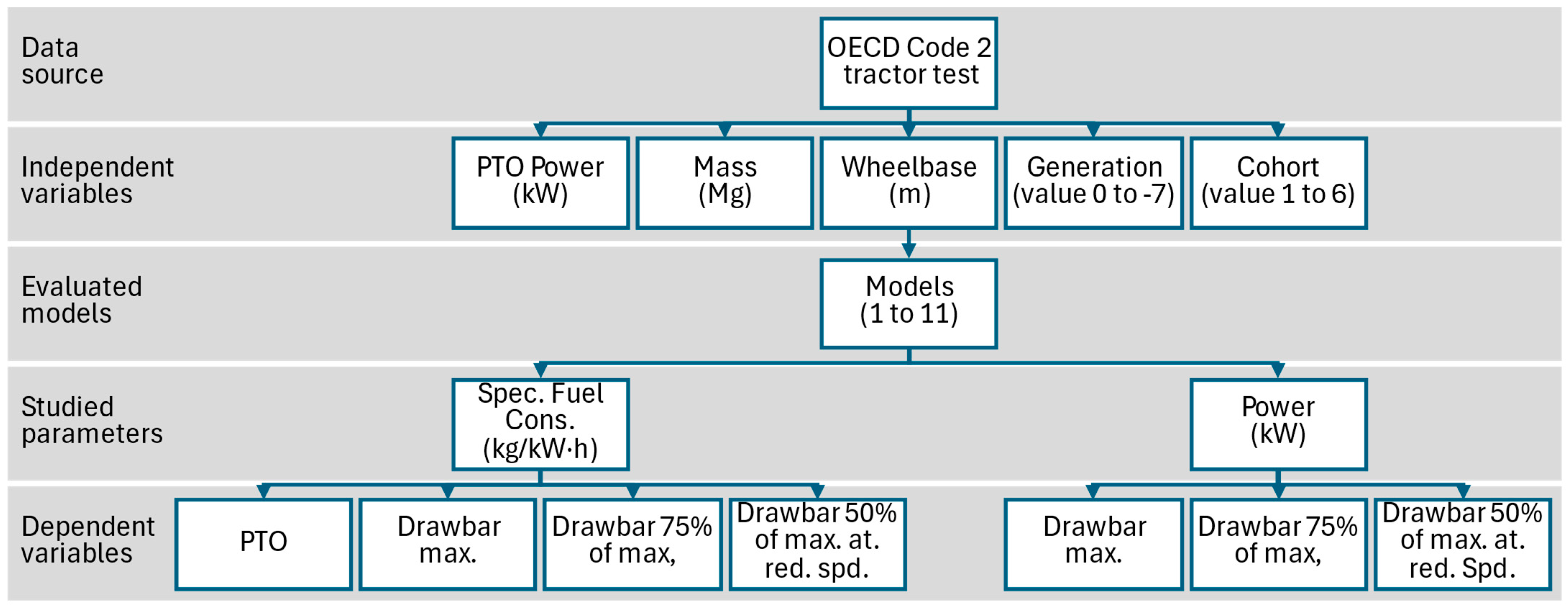
2.1. Dataset

The OECD tractor tests provide a globally recognized, standardized framework for assessing the performance, efficiency, and safety of agricultural tractors. These tests encompass engine power, fuel consumption, traction, hydraulics, and safety under controlled conditions, ensuring both reproducibility and comparability. The insights derived from these tests are invaluable, supporting informed decision-making by farmers, purchasers, and policymakers, and contributing to market transparency, technological innovation, and sustainability.

Given that not all agricultural tractor manufacturers adhere to the OECD code 2 testing protocol with the same frequency or rigor, it is essential to utilize the test results from those who do, in order to effectively evaluate the productivity and efficiency of manufacturers who do not comply with these standards.

John Deere, Moline, IL, USA, being one of the most active participants in OECD code 2 testing—both in terms of the quantity and diversity of models tested, including various powertrains, and the thoroughness of the tests, considering different engine settings and loads (both ballasted and unballasted)—was selected as the subject of this study. Furthermore, the genealogical stability (consistent production facilities) and traceability of John Deere tractor models, coupled with publicly available, legally binding operator’s manuals, make them particularly well suited for inclusion in this study’s dataset.

The dataset encompasses all 138 John Deere tractors equipped with mechanical forward wheel assist (MFWA) that have undergone OECD code 2 drawbar testing, spanning from 1982 to 2024.

2.2. Data Preparation

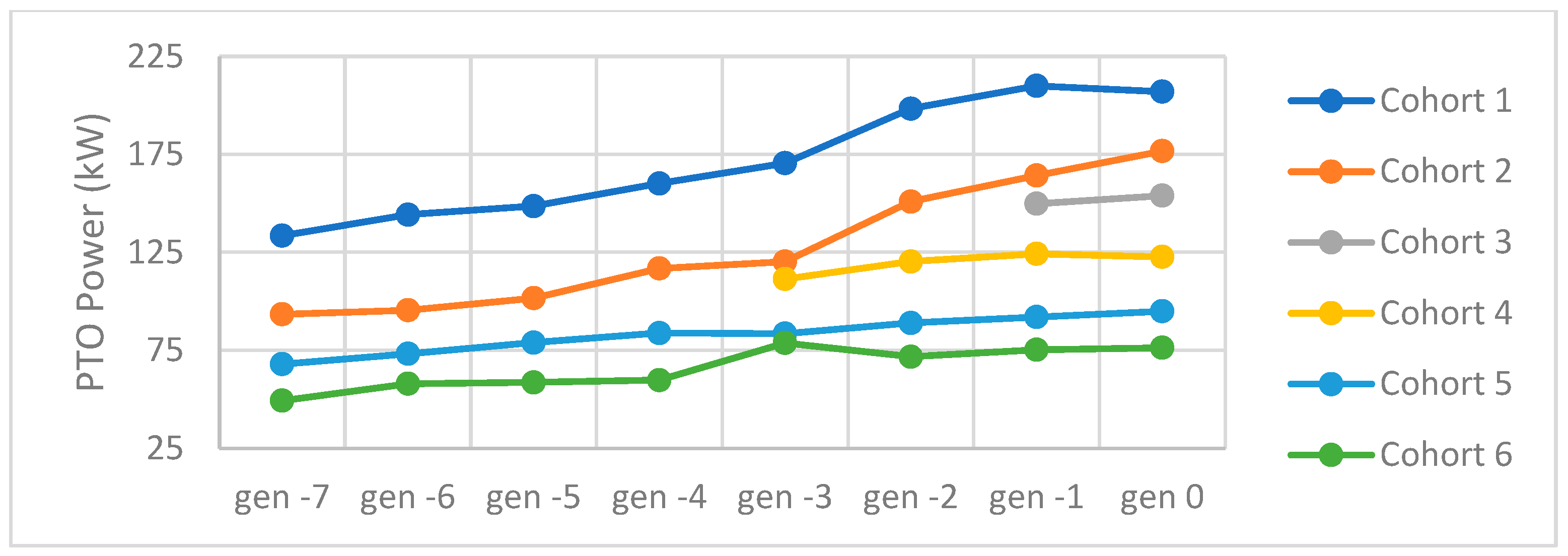
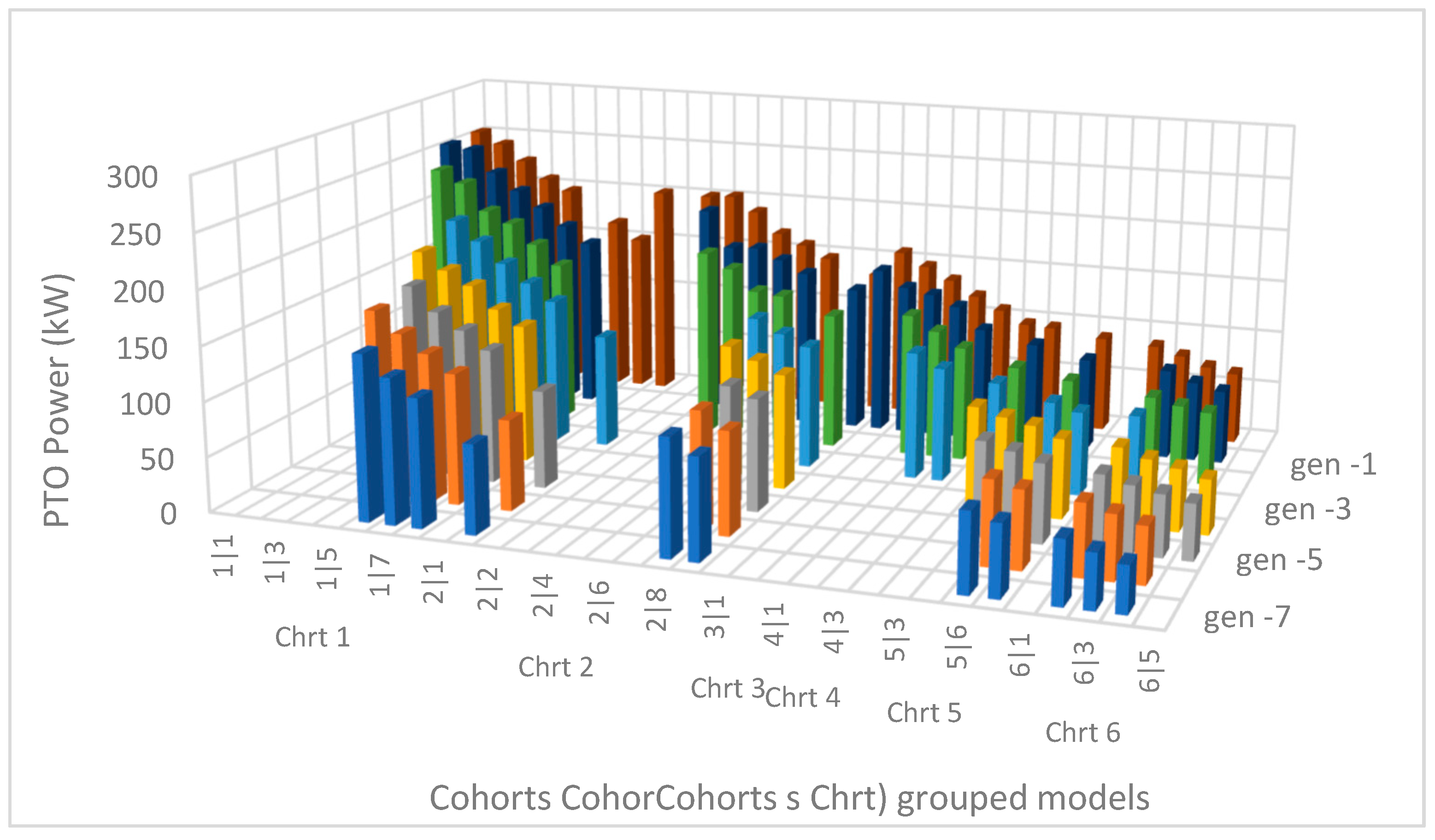
2.2.1. Tractor Cohorts (Chrt)

Original Equipment Manufacturers (OEMs) typically organize their tractor models into series that, while exhibiting common physical characteristics such as size, mass, features, and user interfaces, differ in engine power. In certain instances, these OEM-defined tractor series may encompass a range of models with significantly varying size, mass, and/or features, suggesting the need for further subdivision into cohorts (Chrt) with more homogeneous attributes. The progression of the average wheelbase (m), total mass (Mg), and PTO power (kW) for each generation (see Section 2.2.2) under study is presented in Figure 4, Figure 5 and Figure 6.

As tractors have evolved, becoming larger, heavier, and more powerful, gaps have emerged between models, resulting in increasing differentiation. These gaps were subsequently filled by new tractor cohorts, leading to overlaps in several key attributes. This progression has resulted in a dense and complex tractor portfolio, as illustrated in Figure 7.

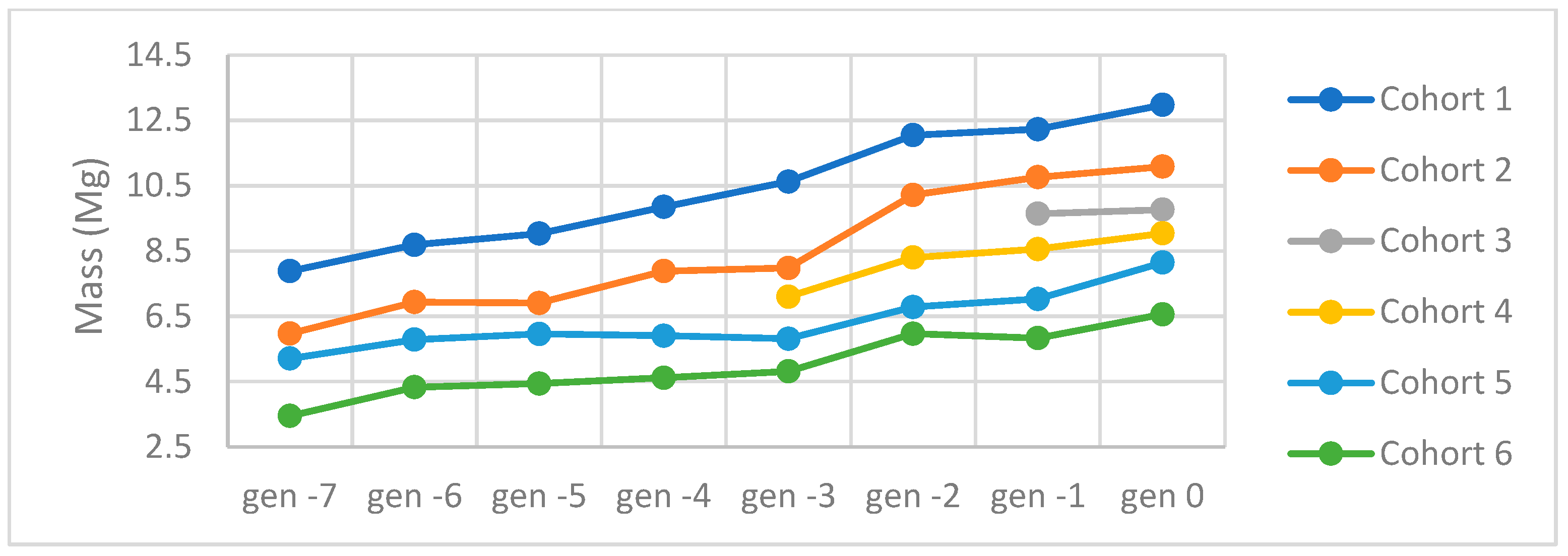
2.2.2. Tractor Generations

The implementation of emission regulations for off-road diesel engines has significantly influenced the release schedules of tractor models. The timeline for these regulations has impacted different power ranges, leading to the synchronization of tractor generations with specific regulatory phases. As a result, the current generation, referred to as Generation 0, includes tractors that are compliant with European Stage V emission standards. Generation-1 comprises those that meet European Stage IV and U.S. Final Tier 4 standards, while Generation-2 includes tractors that conform to Stage IIIb and Interim Tier 4. Generation-3 refers to Stage IIIa- and Tier 3-compliant models, Generation-4 to Stage II- and Tier 2-compliant tractors, and Generation-5 to Stage I- and Tier 1-compliant tractors. Finally, Generation-6 encompasses models that predate the introduction of emission regulations, also known as Stage 0 and Tier 0, with Generation-7 including their immediate predecessors.

Moreover, the need to evaluate the evolution of productivity and, more importantly, efficiency across tractor generations is underscored by the advancements in engine, powertrain, and tire technologies. These developments have not only enabled higher productivity levels but also improved efficiency, which has been further influenced by the implementation of emission reduction technologies, as demonstrated in Figure 8.

2.3. Data Regression

One of the primary motivations for this study is the absence of existing literature that examines the evolution of productivity and efficiency across all emission regulation tiers (ranging from pre-emission standards, or Tier 0, to Final Tier 4). This gap includes an analysis of the effects of implemented technical solutions on various tractor cohorts spanning multiple generations from 1982 to 2024. The analysis of these data facilitated the development of models that describe the evolution of pull power and fuel consumption under different engine settings, considering the impact of the applied technical solutions. Multiple models were constructed to identify an optimal balance between complexity and robustness, aiming to provide the most effective solutions while minimizing cognitive and computational demands.

Linear and polynomial regression are both statistical methods used to model the relationship between a dependent variable and one or more independent variables. Linear regression assumes that the relationship between the dependent variable y and the independent variable x can be described by a straight line. The goal of linear regression is to estimate the values of the coefficients that minimize the sum of squared errors between the observed data and the predicted values. Polynomial regression extends linear regression by fitting a curved relationship between the dependent and independent variables. This method models the relationship as a polynomial of degree n, where the independent variable is raised to higher powers. The coefficients are estimated in a similar way to linear regression, but the higher-degree terms allow the model to capture more complex, nonlinear patterns in the data [40].

Linear regression is ideal for datasets where the relationship between variables is approximately linear, offering simplicity, interpretability, and robustness. It is well suited to scenarios where computational efficiency is essential and the risk of overfitting is low. In contrast, polynomial regression is more appropriate when the relationship between variables is nonlinear and more flexibility is required. However, it comes with the risk of overfitting, increased complexity, and higher computational costs, particularly as the polynomial degree increases. The choice between these two approaches depends on the specific nature of the data and the goals of the analysis [41,42].

In both cases, the fitting process involves minimizing the difference between the observed data and the model’s predictions, typically using techniques like Ordinary Least Squares (OLS), which is a statistical method used in regression analysis to estimate the relationship between a dependent variable and one or more independent variables [43,44]. The goal of OLS is to find the parameter estimates (coefficients) that minimize the sum of squared differences between the observed values and the values predicted by the linear model. Specifically, OLS minimizes the sum of squared residuals, where a residual is the difference between an observed data point and the corresponding predicted value from the regression model [45,46]. This method assumes that the relationship between the dependent and independent variables is linear and that the errors (residuals) are normally distributed with constant variance. OLS provides the Best Linear Unbiased Estimator (BLUE) under the Gauss–Markov assumptions [47].

A graphical summary of the data source, independent variables, evaluated models, studied parameters, and dependent variables can be seen in Figure 9.

The following variables and coefficients have been evaluated in order to determine the specific fuel consumption (kg/kW·h):

• pwr = tested PTO power (kW) at rated engine speed.
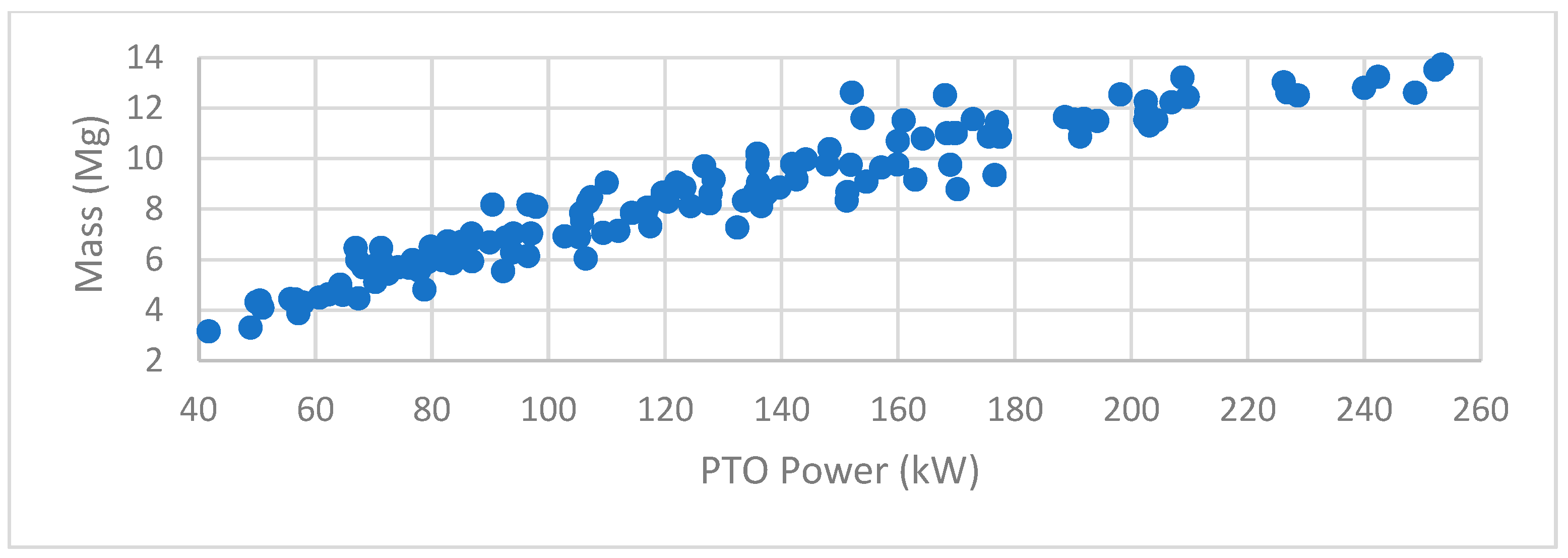
• mss = tested total tractor mass (Mg).
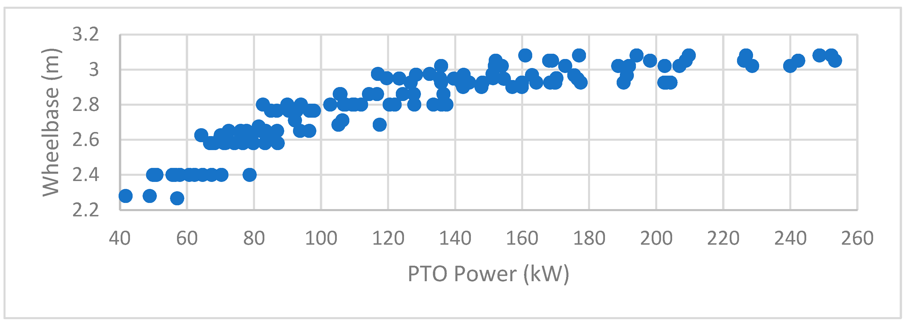
• wbs = tested tractor wheelbase (m).
• generation_i = i tractor generations analyzed in this study (i from 0 to −7 and value 1 or 0).
• cohort_j = j tractor cohorts in which the study tractor population has been grouped (j from 1 to 6 and value 1 or 0).
• coef_pwr1 = coefficient that affects the power.
• coef_pwr2 = coefficient that affects the power².
• coef_mss1 = coefficient that affects the mass.
• coef_mss2 = coefficient that affects the mass².
• coef_wbs1 = coefficient that affects the wheelbase.
• coef_wbs2 = coefficient that affects the wheelbase².
• coef_pwrmss = coefficient that affects the power and mass product.
• coef_pwrwbs = coefficient that affects the power and wheelbase product.
• coef_msswbs = coefficient that affects the mass and wheelbase product.
• y = dependent variable:
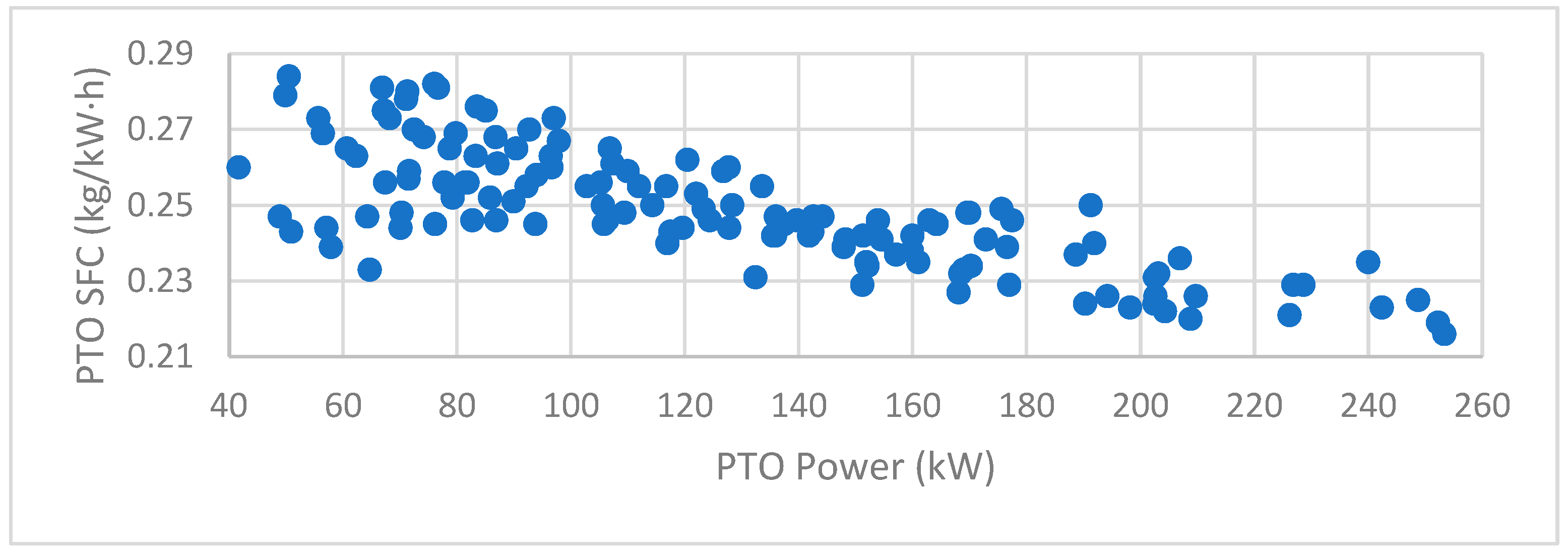
  • Specific fuel consumption (SFC) in kg/kW·h;
  • Drawbar (DB) power in kW.

The following models, summarized in

Table 1. Model independent variables summary (considered binomial are power–mass, power–wheelbase, and mass–wheelbase).

Model	Power	Mass	Wheelbase	Binomial	Generation	Cohorts
1	linear
2	linear	linear	linear
3	poly. 2nd	poly. 2nd	poly. 2nd
4	poly. 2nd	poly. 2nd	poly. 2nd	linear
5	poly. 2nd	poly. 2nd	poly. 2nd	linear (wbs2)
6	poly. 2nd	poly. 2nd	poly. 2nd	linear (mss2)
7	poly. 2nd	poly. 2nd	poly. 2nd	linear (pwr2)
8	linear	linear	linear	linear	linear
9	linear	linear	linear	linear	linear	linear
10	poly. 2nd	poly. 2nd	poly. 2nd	linear	linear	linear
11	poly. 2nd	poly. 2nd	poly. 2nd	linear (mss2)	linear	linear

, have been evaluated:

Model 1:

$$y={coef}_{pwr2}\times {pwr}^2+{coef}_{pwr1}\times pwr+coef$$

(1)

Model 2:

$$y={coef}_{pwr1}\times pwr+{coef}_{mss}\times mss+{coef}_{whb}\times whbs+coef$$

(2)

Model 3:

$$\begin{array}{c}y={coef}_{pwr2}\times {pwr}^2+{coef}_{pwr1}\times pwr+{coef}_{mss2}\times {mss}^2+{coef}_{mss1}\times mss+{coef}_{wbs2}\times {wbs}^2\\ \\ +{coef}_{wbs1}\times wbs+coef\hfill \end{array}$$

(3)

Model 4:

$$\begin{array}{c}y={coef}_{pwr2}\times {pwr}^2+{coef}_{pwr1}\times pwr+{coef}_{mss2}\times {mss}^2+{coef}_{mss1}\times mss+{coef}_{wbs2}\times {wbs}^2\\ +{coef}_{wbs1}\times wbs+{coef}_{pwrmss}\times pwr\times mss+{coef}_{pwrwbs}\times pwr\times wbs\hfill \\ +{coef}_{msswbs}\times mss\times wbs+coef\hfill \end{array}$$

(4)

Model 5:

$$\begin{array}{c}y={coef}_{pwr2}\times {pwr}^2+{coef}_{pwr1}\times pwr+{coef}_{mss2}\times {mss}^2+{coef}_{mss1}\times mss+{coef}_{wbs2}\times {wbs}^2\\ +{coef}_{wbs1}\times wbs+{coef}_{pwrmss}\times pwr\times mss+{coef}_{pwrwbs}\times pwr\times {wbs}^2\hfill \\ +{coef}_{msswbs}\times mss\times {wbs}^2+coef\hfill \end{array}$$

(5)

Model 6:

$$\begin{array}{c}y={coef}_{pwr2}\times {pwr}^2+{coef}_{pwr1}\times pwr+{coef}_{mss2}\times {mss}^2+{coef}_{mss1}\times mss+{coef}_{wbs2}\times {wbs}^2\\ +{coef}_{wbs1}\times wbs+{coef}_{pwrmss}\times pwr\times {mss}^2+{coef}_{pwrwbs}\times pwr\times wbs\hfill \\ +{coef}_{msswbs}\times {mss}^2\times wbs+coef\hfill \end{array}$$

(6)

Model 7:

$$\begin{array}{c}y={coef}_{pwr2}\times {pwr}^2+{coef}_{pwr1}\times pwr+{coef}_{mss2}\times {mss}^2+{coef}_{mss1}\times mss+{coef}_{wbs2}\times {pwr}^2\\ +{coef}_{wbs1}\times wbs+{coef}_{pwrmss}\times {pwr}^2\times mss+{coef}_{pwrwbs}\times {pwr}^2\times wbs\hfill \\ +{coef}_{msswbs}\times mss\times wbs+coef\hfill \end{array}$$

(7)

Model 8:

$$y={coef}_{pwr1}\times pwr+{coef}_{mss}\times mss+{coef}_{whb}\times whbs+{coef}_{gi}\times {generation}_i+coef$$

(8)

Model 9:

$$y={coef}_{pwr1}\times pwr+{coef}_{mss}\times mss+{coef}_{whb}\times whbs+{coef}_{gi}\times {generation}_i+{coef}_{cj}\times {cohort}_j+coef$$

(9)

Model 10:

$$\begin{array}{c}y={coef}_{pwr2}\times {pwr}^2+{coef}_{pwr1}\times pwr+{coef}_{mss2}\times {mss}^2+{coef}_{mss1}\times mss+{coef}_{wbs2}\times {pwr}^2\\ +{coef}_{wbs1}\times wbs+{coef}_{gi}\times {generation}_i+{coef}_{cj}\times {cohort}_j+coef\hfill \end{array}$$

(10)

Model 11:

$$\begin{array}{c}y={coef}_{pwr2}\times {pwr}^2+{coef}_{pwr1}\times pwr+{coef}_{mss2}\times {mss}^2+{coef}_{mss1}\times mss+{coef}_{wbs2}\times {pwr}^2\\ +{coef}_{wbs1}\times wbs+{coef}_{pwrmss}\times pwr\times {mss}^2+{coef}_{pwrwbs}\times pwr\times wbs\hfill \\ +{coef}_{msswbs}\times {mss}^2\times wbs+{coef}_{gi}\times {generation}_i+{coef}_{cj}\times {cohort}_j+coef\hfill \end{array}$$

(11)

The same models (1 to 11) have been evaluated for drawbar power prediction (in the same drawbar at maximum power, at 75% of maximum power, and at 50% of maximum power at reduced engine speed).

In evaluating the performance of the model, two metrics have been utilized: the root mean squared error (RMSE) and the coefficient of determination (R²). The RMSE was selected for its ability to express errors in the same units as the outcome variable, thereby facilitating easier interpretation. A model with perfect accuracy would yield an RMSE value of zero. In contrast, R² has been employed to quantify the proportion of variance in the dependent variable that is explained by the regression model [48].

3. Results

The robustness of the models can be observed my means of their respective coefficients of determination (RSq) and root mean squared error (RMSE) corresponding results for specific fuel consumption (kg/kW·h), as seen in

Table 2. Specific fuel consumption (kg/kW·h) evaluated model results.

Model	PTO Pwr Test		DB Max. Pwr		75% Pull @ Max. Pwr		50% Pull @ Red. Spd.
	RSQ	RMSE	RSQ	RMSE	RSQ	RMSE	RSQ	RMSE
1	0.6091	0.0097	0.5998	0.0134	0.6545	0.0178	0.6123	0.0242
2	0.6216	0.0096	0.6318	0.0130	0.6681	0.0175	0.6383	0.0235
3	0.7120	0.0085	0.6591	0.0126	0.6923	0.0171	0.6592	0.0231
4	0.7321	0.0083	0.6814	0.0124	0.7167	0.0166	0.6829	0.0226
5	0.7296	0.0083	0.6783	0.0124	0.7133	0.0167	0.6784	0.0227
6	0.7305	0.0083	0.6810	0.0124	0.7130	0.0167	0.6741	0.0229
7	0.7286	0.0084	0.6693	0.0126	0.7026	0.0170	0.6662	0.0231
8	0.7767	0.0076	0.7223	0.0116	0.7507	0.0156	0.6866	0.0225
9	0.7836	0.0076	0.7580	0.0110	0.7910	0.0146	0.7405	0.0209
10	0.8372	0.0067	0.7810	0.0106	0.8127	0.0140	0.7533	0.0206
11	0.8519	0.0065	0.8123	0.0100	0.8373	0.0132	0.7691	0.0202

, and drawbar power, as seen in

Table 3. Drawbar power (kW) evaluated model results.

Model	DB Max. Pwr		75% Pull @ Max. Pwr		50% Pull @ Red. Spd.
	RSQ	RMSE	RSQ	RSQ	RMSE	RSQ
1	0.9899	4.8068	0.9900	3.7181	0.9809	3.4632
2	0.9902	4.7721	0.9901	3.7246	0.9810	3.4802
3	0.9914	4.5143	0.9914	3.5091	0.9829	3.3437
4	0.9921	4.3873	0.9923	3.3740	0.9837	3.2986
5	0.9921	4.3935	0.9922	3.3812	0.9837	3.2993
6	0.9920	4.4145	0.9921	3.4033	0.9834	3.3262
7	0.9921	4.3873	0.9923	3.3788	0.9837	3.3034
8	0.9925	4.2934	0.9923	3.3885	0.9831	3.3684
9	0.9934	4.1103	0.9932	3.2312	0.9854	3.1949
10	0.9937	4.0534	0.9938	3.1333	0.9860	3.1683
11	0.9943	3.9141	0.9945	3.0012	0.9868	3.1175

, for the power take-off power test (PTO Pwr Test) and drawbar performance test at maximum power (DB Max. Power), 75% of pull at maximum power (75% Pull @ Max. Pwr.), and 50% of pull at reduced engine speed (50% Pull @ Red. Sped.)

The analysis of the specific fuel consumption (SFC) for various models across different operational conditions is presented in Table 2. The models were evaluated under four distinct scenarios: PTO Power Test, BD Maximum Power, 75% Pull at Maximum Power, and 50% Pull at Reduced Speed. For each scenario, the coefficient of determination (RSQ) and root mean square error (RMSE) were calculated to assess model fit and prediction accuracy.

In general, the results indicate a significant variation in model performance across the evaluated conditions. For the PTO Power Test scenario, model 11 exhibited the highest RSQ value (0.8519), followed by model 10 (0.8372), suggesting that these models provided the best fit for this particular condition. In contrast, model 1 showed the lowest RSQ value (0.6091), indicating a weaker fit relative to other models.

For BD Maximum Power, model 11 again demonstrated superior performance, with the highest RSQ of 0.8123 and the lowest RMSE of 0.0100. Models 8 and 9 also displayed strong results in this condition, with RSQ values of 0.7223 and 0.7580, respectively. On the other hand, Models 1 and 2 yielded relatively lower RSQ values, indicating less accurate predictions for this scenario.

The 75% Pull at Maximum Power scenario followed a similar trend, with model 9 achieving the highest RSQ value (0.7910), closely followed by model 11 (0.8373). The RMSE values for these models were relatively low, further supporting their accuracy. Models 1 and 2, however, demonstrated the least favorable results, with RSQ values of 0.6545 and 0.6681, respectively.

For the 50% Pull at Reduced Speed scenario, model 9 showed the best performance, with an RSQ value of 0.7405 and RMSE of 0.0209. Notably, the performance across all models in this scenario was consistent, with only slight variations in the RSQ values ranging from 0.6123 (model 1) to 0.7691 (model 11). Models 1 and 2 again exhibited lower RSQ values, indicating less precise predictions compared to the higher-performing models.

In summary, models 9, 10, and 11 generally outperformed the others across all test conditions, with model 11 showing the best overall performance in terms of both RSQ and RMSE. These findings suggest that these models provide the most reliable estimates of specific fuel consumption across different operational scenarios. However, further refinement of the models, particularly for lower-performing scenarios such as PTO Power Test and BD Maximum Power, could enhance prediction accuracy.

The evaluated models demonstrated varying degrees of prediction accuracy across different operational conditions, as shown in Table 3. The performance of each model was assessed using key statistical metrics, including the coefficient of determination (RSQ) and root mean square error (RMSE) for three distinct pulling conditions: maximum drawbar power (DB Max. Pwr), 75% pull at maximum power (75% Pull @ Max. Pwr), and 50% pull at reduced speed (50% Pull @ Red. Spd.).

Model 1 exhibited an RSQ of 0.9899 for maximum drawbar power, with an RMSE of 4.8068 kW, and demonstrated strong predictive accuracy across the other two conditions. The RSQ values for the 75% pull at maximum power and 50% pull at reduced speed were 0.9900 and 0.9809, respectively, with corresponding RMSE values of 3.7181 kW and 3.4632 kW.

Models 2 through 11 consistently improved upon the initial model, achieving higher RSQ values and lower RMSE values across all conditions. Model 2 recorded a slight improvement with an RSQ of 0.9902 (DB Max. Pwr) and a corresponding RMSE of 4.7721 kW, which was followed by model 3, with RSQ values of 0.9914 and RMSE of 4.5143 kW, reflecting an enhanced fit for both DB Max. Pwr and 75% Pull @ Max. Pwr. Model 4 demonstrated further improvement with RSQ values reaching 0.9921 and 0.9923, and RMSE values of 4.3873 kW and 3.3740 kW, respectively.

The highest levels of accuracy were achieved with Models 9, 10, and 11. Specifically, model 9 exhibited an RSQ of 0.9934 for DB Max. Pwr and an RMSE of 4.1103 kW. Models 10 and 11 further optimized prediction accuracy, with model 11 reaching an RSQ of 0.9943 for DB Max. Pwr and RMSE values as low as 3.9141 kW. Additionally, model 11 achieved RSQ values of 0.9945 and 0.9868 for the 75% Pull @ Max. Pwr and 50% Pull @ Red. Spd., respectively, with corresponding RMSE values of 3.0012 kW and 3.1175 kW, indicating highly accurate predictions across all conditions.

The data indicate that incorporating BD Maximum Power into the predictive models significantly enhances the accuracy of power prediction across all evaluated conditions. Model 11, with the highest RSQ and lowest RMSE values across the board, provides the most reliable predictions for drawbar power under varying operational scenarios. These results suggest that further refinement of the model with additional parameters may yield even greater predictive performance in future work.

4. Discussion

The OECD tractor test offers significant advantages, providing high-quality, accessible data that add considerable value to the field of agronomy, and by extension, to society. The development of data-driven methodologies is inherently beneficial, with the impact being significantly enhanced when these methodologies are high-quality, transparent, and publicly accessible.

Incorporating additional variables, such as wheelbase and mass (model 2), alongside the traditionally considered PTO power (model 1), enhances both the R-squared (RSq) and root mean square error (RMSE) for specific fuel consumption and drawbar power across all evaluated engine load and speed settings—namely, maximum power, 75% of maximum power, and 50% of maximum power at reduced engine speeds. Even when these variables are included linearly, improvements are evident (PTO Power Specific Fuel Consumption RSq from 0.6091 to 0.6216).

When wheelbase and mass are introduced into the regression as second-degree polynomial terms alongside PTO power (model 3), the robustness of the model improves across all dependent variables. Further, incorporating a binomial relationship between wheelbase, mass, and PTO power leads to additional improvements in the RSq and RMSE values, simultaneously optimizing the studied parameters (model 4 to 7) (PTO Power Specific Fuel Consumption RSq from 0.9914 to 0.9921).

Grouping the tractors by technological generation (model 8) and incorporating these groups into the regression model enhances the predictive accuracy of previous models. However, this effect is surpassed when tractors are additionally grouped by physical attributes-based cohorts (model 9) and added linearly to the regression model, with a more substantial improvement observed when these attributes are introduced in a second-degree polynomial form (model 10) (PTO Power Specific Fuel Consumption RSq from 0.9925 to 0.9937).

The inclusion of binomial variables representing the interaction between wheelbase, mass, and PTO power further strengthens the robustness of the regression model. Notably, when this binomial relationship includes the squared term for mass, it results in the highest levels of model robustness among all the tested configurations (model 11) (PTO Power Specific Fuel Consumption RSq of 0.8519) (See Appendix A for coefficients).

It was anticipated that specific fuel consumption for PTO power would yield the best R-squared (RSq) and root mean square error (RMSE) values, as drawbar power involves dynamic and cinematic variables that are absent in stationary PTO power.

It is noteworthy that the evaluated models demonstrate a greater ability to accurately describe drawbar power behavior at 75% of maximum pull bar power (75% Pull @ Max. Pwr), compared to when assessing maximum pull bar power (BD Max. Pwr). This indicates a higher level of precision in the model’s performance at this intermediate load. Conversely, the model’s ability to describe drawbar power at 50% of maximum pull bar power at reduced engine speed (50% Pull @ Red. Spd.), while still robust, was somewhat less precise, which is expected due to the inclusion of an additional variable, engine speed, in the analysis (RSq of 0.9945, 0.9943 and 0.9868).

The methodology and model presented offer a more robust assessment of specific fuel consumption, thereby justifying the necessity for generation and cohort grouping. This approach contrasts with the analysis of drawbar power, where such grouping may not be as critical. In cases where isolated analyses are required, a less variable, alternative model may suffice.

Future Stydie Recommendations

The methodology employed in the current study primarily focuses on analyzing the evolution of tractor performance and efficiency, from pre-Tier 1 to the current Final Tier 4 standards, in the context of drawbar pull applications as defined by OECD code 2 tractor tests. As such, the scope of the study does not extend to detailed predictions of fuel consumption at specific engine loads and speed settings, including idle and load conditions.

Future research could expand on this by investigating other power take-off systems, such as hydraulic or electric power outputs once these systems have been independently tested in accordance with OECD code 2 equivalents. It would be valuable to examine these power take-offs as well as drawbar pull under various workload scenarios, including intermediate, fixed, or cyclic operations, to better understand their impact on fuel consumption and overall tractor efficiency as well as vehicle emissions. Moreover, future studies could explore different operational conditions, potentially incorporating a broader range of performance scenarios to more comprehensively model tractor energy usage across diverse applications.

5. Conclusions

The proposed methodology is grounded in publicly available, high-quality data from the OECD tractor test, facilitating a robust and transparent dataset that ensures data accessibility and openness (1). This approach incorporates size-related attributes, such as wheelbase and mass, alongside the traditionally used power take-off (PTO) measured power, thereby enhancing the model’s robustness by addressing the increasing density and complexity of the tractor portfolio (2). Furthermore, the methodology categorizes tractors into size-based cohorts and technology-based generations, which further strengthens the model’s robustness (3).

The selected model demonstrates superior robustness, as evidenced by the highest R-squared (RSq) values and the lowest root mean square error (RMSE) for key performance indicators, such as drawbar power (productivity) and specific fuel consumption (efficiency), both at the PTO and drawbar (4). Additionally, the model offers flexibility in application by evaluating performance at various operational levels: maximum power, 75% of maximum power, and 50% of maximum power at reduced engine speeds (5).

The simplicity of the methodology, in turn, enhances ease of use, broadening stakeholder accessibility by reducing cognitive demands and computational power requirements (6). This model enables stakeholders to make data-driven decisions by facilitating the conversion of productivity and efficiency analyses for tractors with diverse characteristics, including size, mass, PTO power, and age (7).

Incorporating additional tractor OEMs that offer OECD tractors under this methodology and model would enhance the state of the art. Furthermore, employing non-parametric models to address the limitations in data quantity and quality would further improve the robustness of the analysis.

References

1. Renius, K.T. Fundamentals of Tractor Design; Springer: Cham, Switzerland, 2020. [Google Scholar]
2. Zoz, F.M.; Grisso, R.D. Traction and Tractor Performance; American Society of Agricultural Engineers: St. Joseph, MI, USA, 2003; Volume 27. [Google Scholar]
3. Brixius, W.W.; Zoz, F.M. Tires and Tracks in Agriculture; SAE Transactions: St. Joseph, MI, USA, 1976; pp. 2034–2044. [Google Scholar]
4. Grisso, R.D.; Kocher, M.F.; Vaughan, D.H. Predicting Tractor Fuel Consumption. Appl. Eng. Agric. 2004, 20, 553–561. [Google Scholar] [CrossRef]
5. Grisso, R.D.; Perumpral, J.V.; Vaughan, D.H.; Roberson, G.T.; Pitman, R.M. Predicting Tractor Diesel Fuel Consumption; Virginia Coopertive Extension: Blacksburg, VA, USA, 2010. [Google Scholar]
6. Stephens, L.E.; Spencer, A.D.; Floyd, V.G.; Brixius, W.W. Energy Requirements for Tillage and Planting. ASAE Tech. Pap. 1981, 81, 1512. [Google Scholar]
7. Kastens, T. Farm Machinery Operations Cost Calculations; Kansas State University: Manhattan, KS, USA, 1997. [Google Scholar]
8. Herranz-Matey, I.; Ruiz-Garcia, L. New Agricultural Tractor Manufacturer’s Suggested Retail Price (MSRP) Model in Europe. Agriculture 2024, 14, 342. [Google Scholar] [CrossRef]
9. Herranz-Matey, I.; Ruiz-Garcia, L. A New Method and Model for the Estimation of Residual Value of Agricultural Tractors. Agriculture 2023, 13, 409. [Google Scholar] [CrossRef]
10. Dallmann, T.; Menon, A. Technology Pathways for Diesel Engines Used in Non-Road Vehicles and Equipment; International Council on Clean Transportation (ICCT): Washington, DC, USA, 2016. [Google Scholar]
11. EPA. Control of Emissions of Air Pollution From Nonroad Diesel Engines and Fuel; Final Rule. U.S. Environ. Prot. Agency (EPA) Fed. Regist. 2004, 69, 4213. [Google Scholar]
12. EPA. Control of Emissions of Air Pollution From Nonroad Diesel Engines; Final Rule. U.S. Environ. Prot. Agency (EPA) Fed. Regist. 1998, 63, 56968–57023. [Google Scholar]
13. EPA. Determination of Significance for Nonroad Sources and, Emission Standards for New Nonroad Compression-Ignition Engine At or Above 37 Kilowatts; Final Rule. U.S. Environ. Prot. Agency (EPA) Fed. Regist. 1994, 59. [Google Scholar]
14. EC. Directive 97/68/EC of the European Parliament and of the Council of 16 December 1997; European Commission (EC): Brussels, Belgium, 1997. [Google Scholar]
15. EC. Directive 2000/25/EC of the European Parliament; European Commission (EC): Brussels, Belgium, 2000. [Google Scholar]
16. EC. Directive 2004/26/EC of the European Parliament and of the Council of 21 April 2004 Amending Directive 97/68/EC; European Commission (EC): Brussels, Belgium, 2004. [Google Scholar]
17. EC. Directive 2009/30/EC of the European Parliament and of the Council of 23 April 2009 Amending Directive 98/70/EC; European Commission (EC): Brussels, Belgium, 2009. [Google Scholar]
18. Janulevičius, A.; Juostas, A.; Čiplienė, A. Estimation of Carbon-Oxide Emissions of Tractors during Operation and Correlation with the Not-to-Exceed Zone. Biosyst. Eng. 2016, 147, 117–129. [Google Scholar] [CrossRef]
19. Larsson, G.; Hansson, P.-A. Environmental Impact of Catalytic Converters and Particle Filters for Agricultural Tractors Determined by Life Cycle Assessment. Biosyst. Eng. 2011, 109, 15–21. [Google Scholar] [CrossRef]
20. Janulevičius, A.; Juostas, A.; Pupinis, G. Engine Performance during Tractor Operational Period. Energy Convers. Manag. 2013, 68, 11–19. [Google Scholar] [CrossRef]
21. Lovarelli, D.; Fiala, M.; Larsson, G. Fuel Consumption and Exhaust Emissions during On-Field Tractor Activity: A Possible Improving Strategy for the Environmental Load of Agricultural Mechanisation. Comput. Electron. Agric. 2018, 151, 238–248. [Google Scholar] [CrossRef]
22. Bacenetti, J.; Lovarelli, D.; Facchinetti, D.; Pessina, D. An Environmental Comparison of Techniques to Reduce Pollutants Emissions Related to Agricultural Tractors. Biosyst. Eng. 2018, 171, 30–40. [Google Scholar] [CrossRef]
23. Reckleben, Y.; Trefflich, S.; Thomsen, H. Impact of Emission Standards on Fuel Consumption of Tractors in Practical Use. Environ. Eng. 2014, 322–326. [Google Scholar]
24. Lovarelli, D.; Bacenetti, J. Exhaust Gases Emissions from Agricultural Tractors: State of the Art and Future Perspectives for Machinery Operators. Biosyst. Eng. 2019, 186, 204–213. [Google Scholar] [CrossRef]
25. Posada, F.; Isenstadt, A.; Badshah, H. Estimated Cost of a Diesel Emissions-Control Technology to Meet Future California Low NOx Standards in 2024 and 2027; The International Council of Clean Transportation: Washington, DC, USA, 2020. [Google Scholar]
26. Posada, F.; Chambliss, S.; Blumberg, K. Cost of Emission Reduction Technologies for Heavy Duty Diesel Vehicles; The International Council on Clean Transportation (ICCT): Washington, DC, USA, 2016. [Google Scholar]
27. Kienzle, J.; Ashburner, J.E.; Sims, B.G. Mechanization for Rural Development: A Review of Patterns and Progress from around the World. Integr. Crop Manag. 2013, 20. [Google Scholar]
28. Fitzgerald, D. Beyond Tractors: The History of Technology in American Agriculture. Technol. Cult. 1991, 32, 114–126. [Google Scholar] [CrossRef]
29. Olmstead, A.; Rhode, P. The Diffusion of the Tractor in American Agriculture: 1910-60; National Bureau of Economic Research: Cambridge, MA, USA, 2000. [Google Scholar]
30. Gray, R.B. Development of the Agricultural Tractor in the United States; American Society of Agricultural Engineers: St. Joseph, MI, USA, 1956. [Google Scholar]
31. White, W.J. Economic History of Tractors in the United States; Whaples, R., Ed.; EH. Net. Encyclopedia: La Crosse, WI, USA, 2001. [Google Scholar]
32. Leffingwell, R. John Deere: A History of the Tractor; Voyageur Press: Floodwood, MN, USA, 2006; ISBN 1610606515. [Google Scholar]
33. Wik, R.M. Henry Ford’s Tractors and American Agriculture. Agric. Hist. 1964, 38, 79–86. [Google Scholar]
34. Duarte, V.; Sarkar, S. A Cinderella Story: The Early Evolution of the American Tractor Industry; CEFAGE-UE Working Paper; University of Evora: Évora, Portugal, 2009. [Google Scholar]
35. Dahlstrom, N. Tractor Wars: John Deere, Henry Ford, International Harvester, and the Birth of Modern Agriculture; BenBella Books: Dallas, TX, USA, 2022; ISBN 1953295746. [Google Scholar]
36. Kim, K.U.; Bashford, L.L.; Sampson, B.T. Improvement of Tractor Performance. Appl. Eng. Agric. 2005, 21, 949–954. [Google Scholar] [CrossRef]
37. Díaz Lankenau, G.F.; Winter, A.G. An Engineering Review of the Farm Tractor’s Evolution to a Dominant Design. J. Mech. Des. 2019, 141, 031107. [Google Scholar] [CrossRef]
38. Bietresato, M.; Mazzetto, F. A Reasoned Evolutionary Study on the Actual Design of Farm Tractors. In Proceedings of the Creative Solutions for a Sustainable Development: 21st International TRIZ Future Conference, TFC 2021, Bolzano, Italy, 22–24 September 2021; Proceedings 21. Springer: Berlin/Heidelberg, Germany, 2021; pp. 256–275. [Google Scholar]
39. Grisso, R.D. Gear up and Throttle Down. 2001. Available online: https://www.pubs.ext.vt.edu/442/442-450/442-450.html (accessed on 1 January 2025).
40. Maulud, D.; Abdulazeez, A.M. A Review on Linear Regression Comprehensive in Machine Learning. J. Appl. Sci. Technol. Trends 2020, 1, 140–147. [Google Scholar] [CrossRef]
41. Heiberger, R.M.; Neuwirth, E.; Heiberger, R.M.; Neuwirth, E. Polynomial Regression. R Through Excel. A Spreadsheet Interface Stat. Data Anal. Graph. 2009, 269–284. [Google Scholar]
42. Ostertagová, E. Modelling Using Polynomial Regression. Procedia Eng. 2012, 48, 500–506. [Google Scholar] [CrossRef]
43. Zuev, K. Statistical Inference. Political Methods: Quantitative Methods eJournal 2016. Available online: https://ssrn.com/abstract=3125891 (accessed on 18 February 2018).
44. Lim, J.S.; Kim, Y.D.; Woo, J.-C. Approximated Uncertainty Propagation of Correlated Independent Variables Using the Ordinary Least Squares Estimator. Molecules 2024, 29, 1248. [Google Scholar] [CrossRef] [PubMed]
45. Dette, H.; Pepelyshev, A.; Zhigljavsky, A.A. Best Linear Unbiased Estimators in Continuous Time Regression Models. arXiv 2016, arXiv:1611.09804. [Google Scholar]
46. Lei, L.; Wooldridge, J. What Estimators Are Unbiased For Linear Models? arXiv 2022, arXiv:2212.14185. [Google Scholar]
47. Hallin, M. Gauss–Markov Theorem in Statistics; Springer: Berlin/Heidelberg, Germany, 2014. [Google Scholar]
48. McCarthy, R.V.; McCarthy, M.M.; Ceccucci, W.; Halawi, L. Applying Predictive Analytics; Springer International Publishing: Cham, Switzerland, 2019; ISBN 978-3-030-14037-3. [Google Scholar]
Figure 1. Power take-off (PTO) power (kW) and wheelbase (m) in studied MFWA tractor testing according to Organization for Economic Co-operation and Development (OECD) code 2 since 1983.
Agriculture 15 00354 g001
Figure 2. PTO power (kW) and total mass (Mg) in studied MFWA tractor testing according to OECD code 2 since 1983.
Agriculture 15 00354 g002
Figure 3. PTO specific fuel consumption (kg/kW·h) in studied MFWA tractor testing according to OECD code 2 since 1983.
Agriculture 15 00354 g003
Figure 4. MFWA tractor wheelbase (m) generational (gen) evolution grouped by cohort as testing according to OECD code 2.
Agriculture 15 00354 g004
Figure 5. MFWA tractor total mass (Mg) generational (gen) evolution grouped by cohort as testing according to OECD code 2.
Agriculture 15 00354 g005
Figure 6. MFWA tractor PTO power (kW) at rated engine speed generational (gen) evolution grouped by cohort as testing according to OECD code 2.
Agriculture 15 00354 g006
Figure 7. MFWA tractor PTO power (kW) at rated engine speed evolution grouped by model and cohorts (Chrt) and generations (gen) as tested according to OECD code 2.
Agriculture 15 00354 g007
Figure 8. MFWA tractor specific fuel consumption (kg/kW·h) during PTO test at rated engine speed generational evolution grouped by cohort as testing according to OECD code 2.
Agriculture 15 00354 g008
Figure 9. Materials and methods graphical summary.
Agriculture 15 00354 g009