Article

Capsicum Counting Algorithm Using Infrared Imaging and YOLO11

by
Enrico Mendez
,
Jesús Arturo Escobedo Cabello
*,
Alfonso Gómez-Espinosa
,
Jose Antonio Cantoral-Ceballos
and
Oscar Ochoa
School of Engineering and Sciences, Tecnologico de Monterrey, Monterrey 64700, NL, Mexico
*
Author to whom correspondence should be addressed.
Agriculture 2025, 15(24), 2574; https://doi.org/10.3390/agriculture15242574
Submission received: 22 October 2025 / Revised: 25 November 2025 / Accepted: 28 November 2025 / Published: 12 December 2025
(This article belongs to the Section Artificial Intelligence and Digital Agriculture)

Abstract

Fruit detection and counting is a key component of data-driven resource management and yield estimation in greenhouses. This work presents a novel infrared-based approach to capsicum counting in greenhouses that takes advantage of the light penetration of infrared (IR) imaging to enhance detection under challenging lighting conditions. The proposed capsicum counting pipeline integrates the YOLO11 detection model for capsicum identification and the BoT-SORT multi-object tracker to track detections across a video stream, enabling accurate fruit counting. The detector model is trained on a dataset of 1000 images, with 11,916 labeled capsicums, captured with an OAK-D pro camera mounted on a mobile robot inside a capsicum greenhouse. On the IR test set, the YOLO11m model achieved an F1-score of 0.82, while the tracker obtained a multiple object tracking accuracy (MOTA) of 0.85, correctly counting 67 of 70 capsicums in a representative greenhouse row. The results demonstrate the effectiveness of this IR-based approach in automating fruit counting in greenhouse environments, offering potential applications in yield estimation.

1. Introduction

Agriculture stands as an industry of central importance, crucial for social stability and economic development worldwide [1,2]. The convergence of increasing food demand and a decreasing agricultural workforce has driven a surge in research projects focused on smart and precision agriculture [2]. This sectoral transformation, called agriculture 4.0, integrates modern information technologies such as the Internet of Things, artificial intelligence, big data, and computer vision, for intelligent control and data-driven decision-making [2].
The arrival of smart agriculture leads to new opportunities for the development of agricultural production, one of which is fruit detection, which is needed to perform more complex implementations such as fruit counting [3], fruit harvesting [4,5], or yield prediction [6].
Fruit detection not only allows the implementation of these complex tasks, but also allows the estimation of how many pieces of fruit a greenhouse will produce while providing information on the stage and growth state for each fruit, both relevant for a greenhouse administrator [7].
Standard methods for fruit counting are usually based on computer vision or machine learning. Computer vision (CV) is a multidisciplinary field that addresses how computers can understand the content of videos and images [8]. Consequently, traditional CV algorithms have been extensively utilized in the development of fruit perception methods, with the primary advantage being low computational demands due to the simplicity of some of these algorithms [9]. These algorithms use visual sensors to gather image data and three-dimensional coordinates of targets [9], such as the research presented by Lin et al. [10], based on a detection algorithm that focuses on color, shape, and depth characteristics to detect fruits in a natural environment.
Recently, research has focused on deep learning (DL) for fruit detection and segmentation. Unlike traditional CV algorithms, which are based on explicit feature engineering, DL methods enable automatic feature extraction without manual intervention [11]. Therefore, these algorithms can automatically identify the optimal features for training, facilitating effective pattern detection and improving generalization.
Deep learning, a subset of machine learning, employs artificial neural networks (ANN), such as convolutional neural networks (CNN), which incorporate convolutional layers [12]. Since 2012, CNNs have become the leading approach to address computer vision problems due to their outstanding performance [13,14]. They have also been widely used for segmentation tasks in agricultural environments because of their ability to detect objects among noisy backgrounds and their resilience to variations in lighting, usually lacking in non-DL algorithms [11]. Nevertheless, these advantages come with a trade-off, since deep learning usually requires prior model training, which is both time-consuming and computationally demanding.
Different CNNs have been applied to fruit detection. According to [15], the most widely used methods for fruit detection tasks are based on R-CNN (region-based convolutional neural networks) [16] and YOLO (You Only Look Once) [17]. For instance, Afonso et al. [3] used Mask R-CNN [18] to detect tomatoes in a greenhouse using a stereo camera, and their algorithm segmented front-row fruits from those in the background, achieving an F1-score of 0.83. Likewise, ref. [19] used a Mask R-CNN for passion fruit detection, obtaining an F1-score of 0.94. Other studies have extended these methods to yield estimation, e.g., [20] employed a faster R-CNN model to detect multiple fruits, with F1-scores of 0.9534, 0.9794, 0.9424, 0.9534, and 0.9383 for apples, oranges, tomatoes, pomegranates, and mangoes, respectively. Similarly, ref. [21] achieved 0.90 average precision in a peach detection algorithm using faster R-CNN.
YOLO-based models are another widely used approach for fruit detection. Unlike two-stage detectors such as Faster R-CNN, YOLO directly predicts bounding boxes and class probabilities without requiring a separate regional proposal network [17], resulting in faster inferences. For example, when comparing YOLOv8 with Mask R-CNN for orchard segmentation, Sapkota et al. [22] reported that YOLO achieved better precision and inference speed in single and multiclass segmentation. It also outperformed Mask R-CNN in more challenging conditions, such as scenes with similar color between targets and background, as well as with varying illumination. A recent review of the literature on agricultural object detection, algorithms using YOLO reported that more than 70 % of the reviewed works report an accuracy greater than 90 % [23], setting this indicator as an excellent reference to assess the performance of these models.
YOLO-based algorithms for fruit detection and counting have been tested by several research groups. Bazame et al. [24] developed a coffee fruit detection algorithm using YOLOv3, obtaining an F1-score of 0.82. Chen et al. [25] proposed a real-time apple detection algorithm that consists of a smaller version of YOLOv3, achieving 0.9 recall. By reducing the model’s total number of parameters, the algorithm did not impact the efficiency of harvesting robots. Nonetheless, despite the model’s high recall, it was not able to work under poor illumination conditions such as during the night or under light variations. Similarly, Mirhaji et al. [26] trained and deployed an orange detection algorithm by comparing different versions of YOLO models (v2, v3, and v4), and they obtained results that showed that YOLO v4 performed the best, obtaining an F1-score of 0.92.
Several other research works have presented distinct, tailored YOLO-based models for specific fruits. Gai et al. [27] used a YOLOv4-based model to detect cherries and obtained an F1-score of 0.94; Tsai [28] obtained 0.96 accuracy in a YOLOv5-based model to detect tomatoes; and Du et al. [29] proposed a YOLOv7-based model to detect strawberries that achieved a recall of 0.82.
Effective fruit detection requires specialized machine vision algorithms or deep learning models trained on the unique identification characteristics of the fruit. A fruit that has attracted high interest is capsicum; this is one of the most consumed vegetables in the world [30] and has acquired economic importance as a highly demanded vegetable [31]. This fruit is popular among consumers due to its taste, high nutritional value, and richness in vitamins and minerals.
Similar to other studies, research on capsicum detection has used different approaches to accomplish detection. For Mask R-CNN models, Cong et al. [32] compared the performance of different backbone versions of Mask R-CNN to detect capsicums, and the one that introduces the Swin Transformer attention mechanism outperforms the others, obtaining an F1-score of 0.98 . Nonetheless, the authors state that the algorithm is not suitable for real-time applications, given its slow response time.
Likewise, Lopez-Barrios et al. [33] proposed two Mask R-CNN models, one to detect capsicum and a second one to detect the peduncle of the fruit, with precision rates of 0.84 and 0.71, respectively.
Implementing YOLO-based models, Viveros et al. [34] developed a capsicum counting system that integrates a YOLOv5 detection model and a DeepSORT [35] tracking algorithm, which reached an F1-score of 0.77 at a confidence level of 0.58. Similarly, Paul et al. [12] applied different YOLO models and Supervision algorithms to perform a capsicum counting algorithm, obtaining an average accuracy of 0.92 along the tests it performed. Their model had a detection speed higher than 34 FPS, which is already considered real time [36]; the authors report working with different sensors such as multispectral imaging or LiDAR as future work.
All of these studies highlight the characteristics that make this fruit particularly challenging during field tests: background noise in images, little color variation between the fruit and the leaves and trunks, and the nonregular geometry of the target. To overcome these challenges, different detection modalities have been used in different works.
In addition to traditional RGB cameras, various alternative sensors have been tested in agriculture. While some objects have the same appearance in the visual spectrum, they may exhibit different reflectance in a non-visible spectrum [37]. This leads to varied spectral images that provide data for fruit perception uses. For example, Wu et al. [38] used multispectral photos to estimate the ripeness of peppers, and Zhang et al. [39] used hyperspectral images to detect defects in mandarins. Thermal images use the temperature difference between fruit and foliage to improve the perception of fruit. For instance, Gan et al. [40] combined a thermal camera with a spray system to force a thermal difference between citrus and leaves. In addition, Paul et al. [41] developed a detection algorithm to detect capsicums in a greenhouse environment.
Within the same context of different spectral sensors, infrared (IR) cameras have become a common tool in modern agriculture due to their ability to capture information beyond the visible spectrum (390–700 nm), particularly within the 800 to 2500 nm wavelength range [42]. This technology has proven to be useful for real-time fruit quality assessment due to IR wavelength penetration capacity, making IR cameras a standard tool for detecting fruit defects [43]. For example, ref. [44] presented an apple defect detection system using IR images and [45] applied IR images to detect defects in blueberries. Both studies were conducted in a post-harvest environment.
The light penetration and robustness under low or changing light conditions are key advantages of IR imaging for capsicum detection. Due to the light penetration of the wavelength, IR images can clearly distinguish between green leaves and green capsicums, whereas RGB images often fail. As illustrated in Figure 1, this makes IR images an effective tool for overcoming three challenges in capsicum counting applications: (a) low light due to shadows or illumination, (b) background confusion when capsicums and leaves are of similar color, and (c) occlusion by foliage, where overlapping leaves occlude the capsicums, especially challenging in RGB images.
In this study, we aim to address the research question of whether infrared (IR) images can be used to detect and count capsicums and to identify the associated advantages. To this end, we integrate IR imaging with YOLO11 within the BoT-SORT tracking algorithm to perform a capsicum detection and counting system. YOLO11 was trained on 1000 labeled images collected from a capsicum greenhouse. To evaluate the algorithm’s performance, field tests were conducted in a greenhouse. The YOLO11 model achieved an F1-score of 0.82 and the tracker obtained a multiple object tracking accuracy (MOTA) of 0.85. These results indicate that the IR-based counting algorithm is suitable for capsicum counting applications.
The remaining sections of this paper are structured as follows: Section 2 depicts the different methods used in the work, Section 3 describes the experimental setup, Section 4 details the results obtained in the experiments and their analysis, followed by conclusions in Section 5.

2. Materials and Methods

The typical fruit counting pipeline consists of two operations: an object detection algorithm to identify the presence of fruits in an image and a tracking algorithm to track the number of fruits along a video stream. In this section, the materials and methods implemented for both the detection and tracking of capsicums and the image acquisition methodology are described.

2.1. Object Detection

Object detection is the basis for other computer vision tasks, such as instance segmentation, image classification, class segmentation, and tracking, which is the goal of this work. CNNs have proven to be an effective method for object detection. There are mainly two classes of CNNs for object detection: two-stage detectors composed of a region proposal generator and bounding box prediction, and one-stage detectors that perform classification and bounding box regression without generating proposal regions [46,47]. One-stage detectors such as the YOLO models are optimal for real-time applications due to their faster detection process compared to two-stage ones.
YOLO was proposed by Redmon et al. [17], inspired by a human vision system that only looks once to gather information. As the first detector in the class of one-stage detectors, it reaches inferences at 155 FPS, faster than the two-stage detectors. Later, different versions of the YOLO model were released, each of them improving performance and speed over the previous ones. A comprehensive description of the evolution of the YOLO series is detailed in [48].
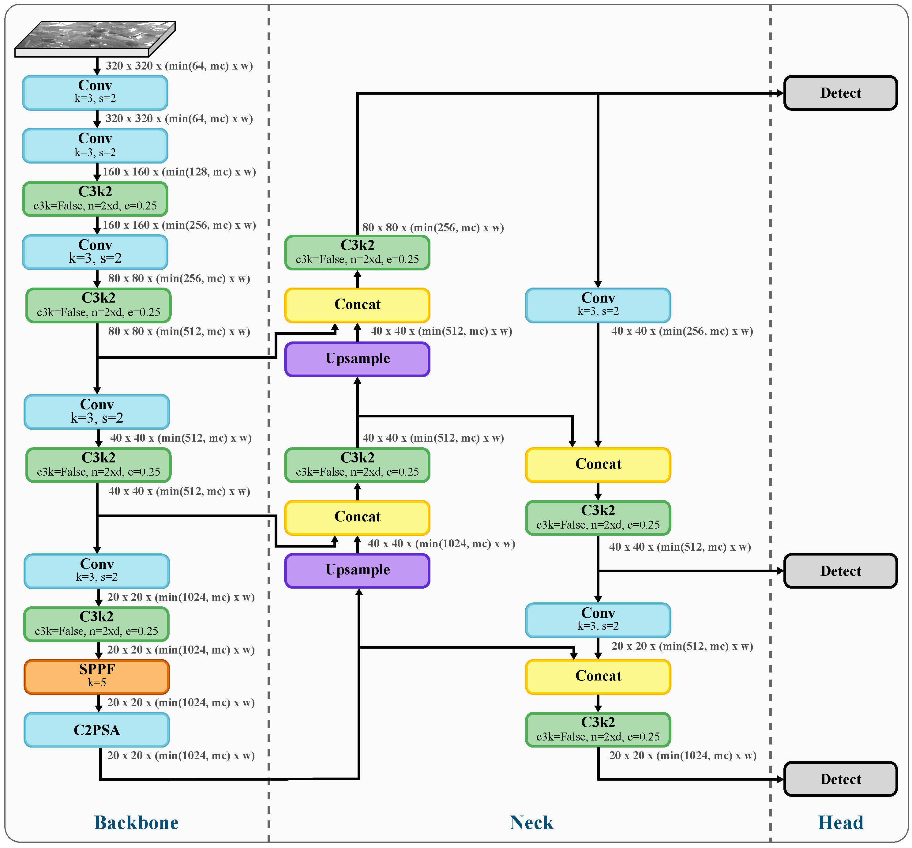
YOLO11, an iteration of the series of YOLO models, was released by Ultralytics in 2024 [49]. This iteration, compared to previous releases, replaces the C2F module, used in YOLOv8, with the C3K2 module in both the backbone and neck of the network. Also, after the SPPF (Spatial Pyramid Pooling–Fast) layer, YOLO11 introduces the C2PSA (Cross-Stage Partial with Parallel Spatial Attention) module, which combines CSP-style channel splitting with pyramid spatial attention to enhance feature extraction from images. Continuing with the idea introduced in YOLOv10, YOLO11 uses an anchor-free, decoupled detection head, where classification and regression branches are separated and implemented with lightweight convolutions [50]. This version also presents a reduction in 20 % of its parameters compared to previous versions, which requires fewer computational resources and makes it suitable for real-time detection applications. This version provides five scaled versions, including nano, small, medium, large, and extra large, and supports the following tasks: object detection, segmentation, pose estimation, oriented detection, and classification.
YOLO 11 incorporates an architectural redesign that results in greater performance with fewer parameters due to better feature extraction [51]. This model architecture is divided into 3 stages: the backbone responsible for feature extraction using convolutional layers to transform an image into multiscale feature maps; the neck that works as an intermediate between the last layers, enhancing feature representations; and finally, the head that serves as a prediction mechanism producing object localization and classification outputs [51]. Figure 2 shows the architecture of YOLO11 and the different variant parameters.

2.2. Tracking Algorithms

The goal of multi-object tracking (MOT) is to determine the paths of numerous objects within a video, and the tracking-by-detection approach has emerged as the most successful paradigm [52]. The tracking-by-detection paradigm consists of a detection stage, usually a detector such as YOLO, followed by a tracking stage [53]. The tracking stage consists of two key components: a motion model and state estimation, which are used to anticipate the bounding boxes of tracklets in subsequent frames. A commonly used method for this purpose is the Kalman filter, and the second component links the new frame detections to the existing track set.
In this work, the BoT-SORT model using YOLO11 was implemented to obtain the number of capsicums detected through a video stream. BoT-SORT [53] is an efficient MOT algorithm that utilizes a state vector based on the Kalman filter and the Hungarian algorithm [54]. Its ability to track numerous targets with a moving camera makes it suitable for agricultural contexts [55].
Figure 2. YOLO11 architecture [17]. Model variant dimension parameters are described in Table 1.
Agriculture 15 02574 g002
Table 1. Model variant parameters with depth, width multiples, and maximum channels.
Model Variantd (Depth_Multiple)w (Width_Multiple)mc (Max_Channels)
n0.500.251024
s0.500.501024
m0.501.00512
l1.001.00512
xl1.001.50512
Figure 3 illustrates the overall workflow of BoT-SORT, which consists of the following: 1. Detection: Detecting objects by obtaining bounding boxes from the YOLO11 model for each frame. 2. Motion estimation: Applying a Kalman filter to estimate the camera motion to predict the positions of the bounding boxes in the next frame, given the previous tracklets. 3. Data Association: Two-stage previous track matching. The first one matches the high confidence detection using the Hungarian algorithm, minimizing a cost function based on proximity and appearance. The second stage matches the remaining detections exclusively using the IoU distance cost function also optimized by the Hungarian algorithm. 4. Track Management: Updating the tracks with newly matched detections and handling unassigned tracks or new detections appropriately.

2.2.1. Kalman Filter for Motion Prediction

A crucial element of BoT-SORT is the Kalman filter, which estimates the movement of objects across consecutive frames. The SORT algorithm defines the state vector composed of the center coordinates of the 2D object, the bounding box area, and the aspect ratio. However, BoT-SORT developers state that estimating the width and height of the bounding box directly leads to better results. Therefore, they define the state vector as in Equation (1) and the measure vector as in Equation (2), where x = [ x c , y c , w , h , x ˙ c , y ˙ c , w ˙ , h ˙ ] is the eight-dimensional Kalman state vector and z = [ z x c , z y c , z w , z h ] is the four-dimensional measurement vector. Here, x c and y c represent the center coordinates of the bounding box on the x and y axes, respectively, w and h denote the width and height of the bounding box, and x ˙ c , y ˙ c , w ˙ and h ˙ are the corresponding velocities of the center coordinates, width, and height. The terms z x c and z y c denote the measured center coordinates provided by the detector, while z w and z h are the measured width and height of the bounding box. In addition, Q and R are made up of functions of some estimated elements and some of the measured ones, resulting in time-dependent matrices. The construction of these matrices is described in the original work [53].
x = x c , y c , w , h , x ˙ c , y ˙ c , w ˙ , h ˙
z = z x c , z y c , z w , z h

2.2.2. Re-Identification and Data Association

Once the predicted states for each tracked object are available, new detections from the YOLO11 model must be assigned to existing tracks. To match detections with tracks, appearance features are employed. These features are extracted using a deep appearance encoder with ResNeSt50 [56] as the backbone. In addition, geometric distance, expressed as the Intersection over Union (IoU) distance between bounding boxes, is used to refine the associations.
BoT-SORT builds a cost matrix C of size N tracks × N detections , where each element C i j represents the probability that the detection j belongs to the predicted track i. The cost matrix is defined as follows:
d ^ i , j cos = 0.5 · d i , j cos , ( d i , j cos < θ emb ) ( d i , j iou < θ iou ) 1 , otherwise
C i , j = min { d i , j iou , d ^ i , j cos } ,
where
  • d ^ i , j cos is the appearance cost.
  • d i , j cos is the cosine distance between the average tracklet appearance descriptor i and the new detection descriptor j.
  • θ emb is the appearance threshold, which is used to separate positive associations of tracklet appearance states and detection embedding vectors from negative ones.
  • θ iou is a proximity threshold, set to 0.5 as in [53], used to reject unlikely pairs of tracklets and detections.
  • d i , j iou represents the motion cost and is the IoU distance between the tracklet i-th predicted bounding box and the j-th detection bounding box.
  • C i , j is the ( i , j ) element of the cost matrix C.
Using the cost matrix C , the association of detections is then performed using the Hungarian algorithm [57].

2.2.3. Integration with YOLO11

By integrating BoT-SORT with the YOLO-based model as a detector for the tracking algorithm, a robust capsicum counting pipeline is obtained. The YOLO-based detector brings the advantages of single-shot detectors such as fast, nearly real-time detection, providing the bounding boxes needed to perform the tracking.
In addition, BoT-SORT provides solutions to the common challenges of using YOLO models in agriculture. For instance, partially occluded fruits might not be detected by the YOLO model during certain frames; however, thanks to the tracking and detection associations, those fruits can be properly linked to a track so that if the fruit is first visible and then occluded by foliage, once it is visible in the frame again, it will only be counted once. In this way, the algorithm counts tracks rather than capsicum instances per frame.

3. Experimental Setup

3.1. Image Acquisition

For this work, RGB and IR capsicum images were captured with an Oak-D Pro camera (Luxonis®, Littleton, CO, USA). The Oak-D Pro is a stereo depth camera that features a color IMX378 12 MP color rolling shutter camera RGB and two OV9282 1MP global shutter monochrome cameras. Both monochrome sensors do not include an IR filter, allowing them to capture visible and IR light, making the Oak-D pro suitable for recording both RGB and IR images simultaneously.
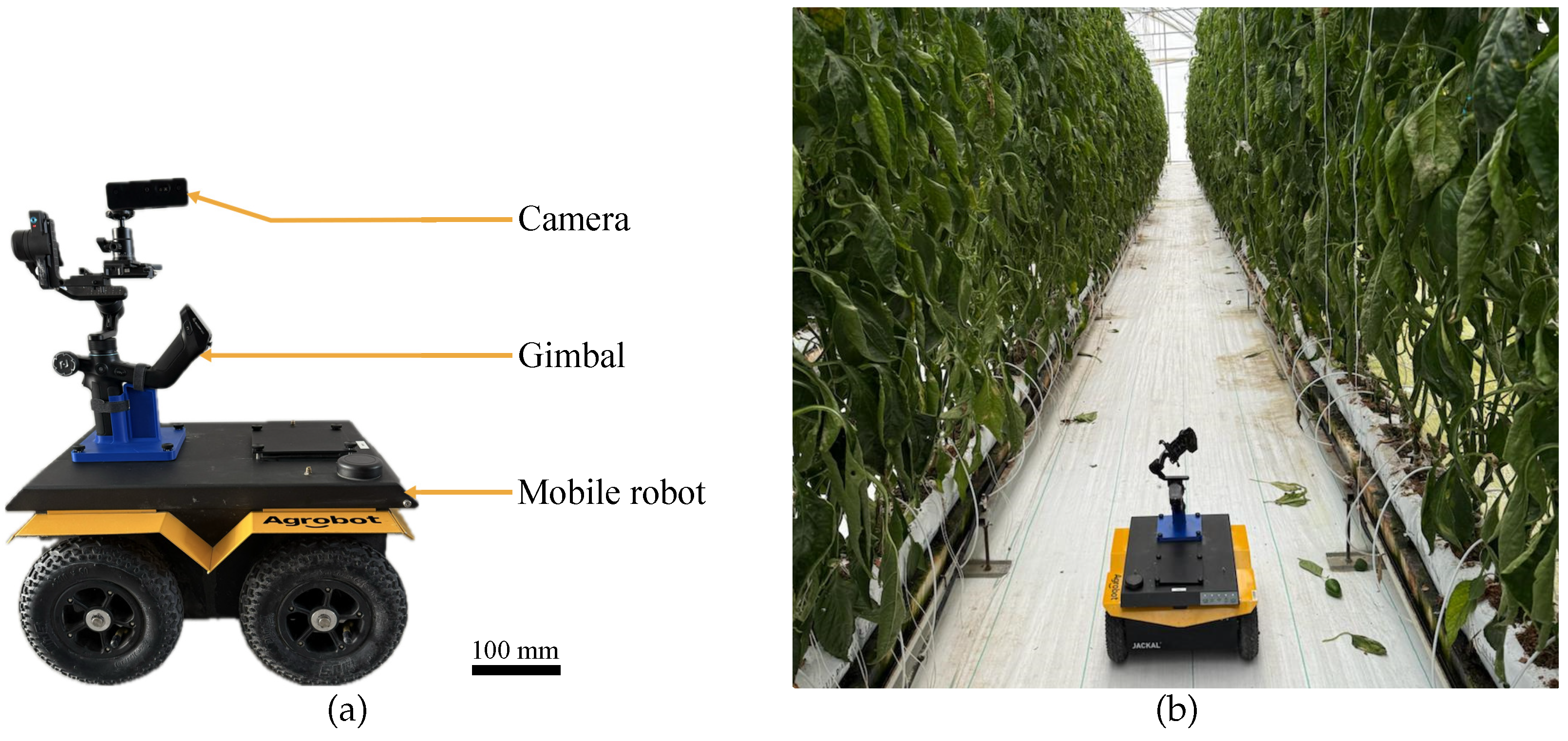
The camera was mounted on a Scorp Mini 2 Gimbal (FeiyuTech, Guilin, Guangxi, China), which was set to stabilize roll and pitch. This gimbal was installed on a Jackal mobile robot (Clearpath Robotics, Kitchener, ON, Canada), as can be seen in Figure 4a. The images used to train and evaluate the models were acquired in a capsicum greenhouse located in CAETEC (Experimental Agricultural Field of the Tecnologico de Monterrey, Qro, Mexico). Figure 4b shows the robot traversing a greenhouse lane.
Ten different greenhouse lanes were recorded by placing the mobile robot in the center of a greenhouse lane, directing the camera to one side facing the plants, and driving the robot through the entire lane at a constant speed of 0.2 m/s. The robot was manually driven, and an external computer was used to run a script to record both IR and RGB videos at 30 frames per second, and stored in three-channel BGR format. Thereby, all the IR images in this work are stored and processed as three-channel images. The IR recordings were captured at a resolution of 1280 × 720 , while the RGB recordings were acquired at 1920 × 1080 .

3.2. Dataset and Model Training

The dataset used to train the detector comprised images extracted from videos taken in the greenhouse at a rate of 5 images per second; then, the capsicums were labeled using the Roboflow platform [58]. The dataset is available at [59].
Labeling is a key stage of our detector model. The better the data are labeled, the more robust the model will generalize. To ensure that all capsicums were accurately annotated in the IR dataset, where grayscale imagery can make object identification challenging, the contrast of each image was individually adjusted using a slider in the labeling software interface. These contrast operations are performed by applying a linear intensity transformation to each pixel of the image, typically expressed as
I adj ( x , y ) = clip α I ( x , y ) + β , 0 , 255 ,
where I ( x , y ) denotes the original pixel intensity at location ( x , y ) , I adj ( x , y ) is the intensity after contrast adjustment, α is a gain factor that controls the contrast (values α > 1 increase contrast, whereas 0 < α < 1 reduce it), and β is an additive offset that shifts the overall brightness of the image (positive β brightens the image and negative β darkens it). The clip ( · ) operator constrains the result to the valid display range [ 0 , 255 ] of 8-bit grayscale images, preventing numerical overflow.
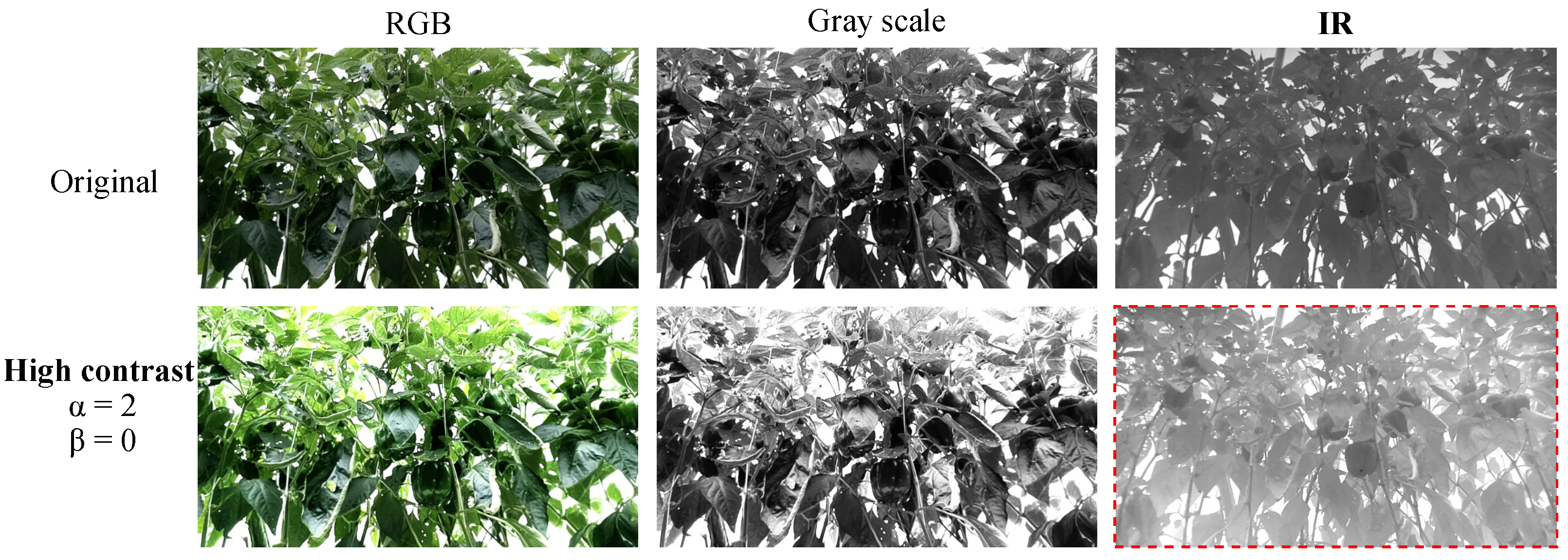
This contrast enhancement increased the visual separation between the capsicums and the background, as illustrated in Figure 5. Figure 5 shows how the adjustment of the contrast in the IR images highlights capsicums, facilitating the labeling process. However, it must be noted that the contrast in the images is only temporarily applied for labeling purposes while the original images are used for training. Figure 5 also shows how contrast adjustments work properly only for IR images, since capsicums are not more noticeable when contrast is adjusted in the original images. It can also be seen that grayscale and IR images are not identical and do not have the same effect when high contrast is applied, since IR provides information on another wavelength.
Training was performed on a local Ubuntu 24.04 workstation equipped with an AMD Ryzen 5 5600X 6-core CPU and an NVIDIA RTX A6000 GPU (NVIDIA, Santa Clara, CA, USA) with 48 GB of VRAM and 64 GB of system RAM. Python 3.11.11 was used to train different YOLO11 models using the Ultralytics and Roboflow libraries [49,58].

3.3. Capsicum Counting

To count the number of capsicums in a video stream, a BoT-SORT tracker is implemented using Python along with the Ultralytics Python library [49]. The settings of the tracker parameters used for the tests are summarized in Table 2.
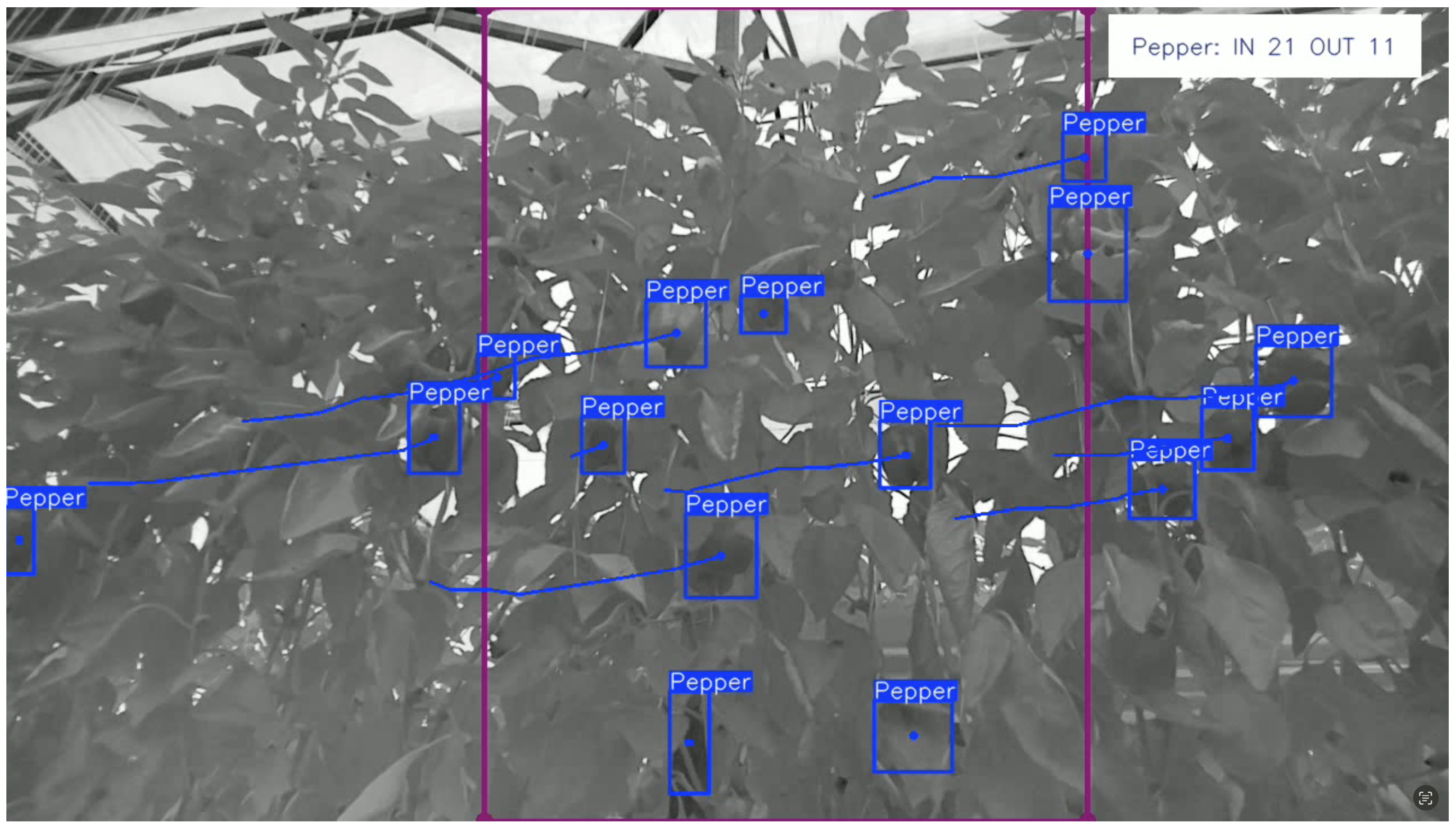
The tracker outputs different tracks showing the trajectory of the different instances detected throughout the video stream. To keep a count of how many capsicums appear in the entire video, a region of the frame is selected, and each time a track appears or goes through the region, a new capsicum is counted.
The region can be defined by either a line or a polygon through which the instances must pass to be counted. For this application, where capsicums may be partially occluded across several frames, a wider region is used to detect new instances. As shown in Figure 6, a central portion of the frame was selected as the counting region. The region was selected so that most capsicums are visible to the camera, with the right side of the frame showing the capsicums before they are covered by foliage, while the center captures the capsicums at their closest positions. Toward the left, i.e., while leaving the frame, other capsicums emerge from foliage or other fruits. Additionally, using a region instead of a line also enables our model to count capsicums that are temporarily occluded by others during a segment of the video. After testing various locations for the counting region, it was defined as a rectangle spanning the entire image height and extending from 0.33 to 0.75 of the frame width.

4. Results and Discussion

4.1. Performance Metrics

To evaluate the performance of the YOLO11-based algorithm for capsicum detection and counting, we employed the most commonly used metrics in related work: accuracy, precision, recall, and F1-score. These metrics are derived from the classification results, which can be categorized as follows.
  • True Positives (TP): The number of correctly identified capsicums.
  • True Negatives (TN): The number of correctly rejected non-capsicum instances, such as foliage or background.
  • False Positives (FP): The number of non-capsicum instances incorrectly identified as capsicums.
  • False Negatives (FN): The number of capsicums that the algorithm failed to identify.
The metrics are defined as follows:
A c c u r a c y = T P + T N T P + T N + F P + F N ;
P r e c i s i o n = T P T P + F P ;
R e c a l l = T P T P + F N .
A close balance between recall and precision typically indicates robust performance. To quantify this balance, the F1-score combines both metrics into a single value and is calculated as follows:
F 1 S c o r e = 2 × P r e c i s i o n × R e c a l l P r e c i s i o n + R e c a l l .
These metrics collectively offer a robust framework for assessing the accuracy, reliability, and stability of the proposed YOLO11-based detection and counting algorithm.
Additionally, the MOTA metric was used to evaluate the tracker’s performance. MOTA also considers errors in object detection, specifically false negatives ( F N ) and false positives ( F P ). It also considers errors in the instance matching, false IDs ( I D S ), which occur when the algorithm switches the ID of the tracked target. MOTA is calculated as in Equation (10), where G T is the number of targets (ground truth) along the video stream. This number was estimated by manually analyzing the video and counting all visible capsicums in the video.
M O T A = 1 F N + F P + I D S G T .

4.2. Object Detection

The detection system carried out by the YOLO11 detection model is evaluated using the test subset of the dataset to calculate the F1-score. To ensure obtaining the best possible model, different sizes of the YOLO11 model were trained.
Two distinct model configurations were trained: one using IR imagery and the other using RGB imagery. The IR dataset comprised frames extracted from greenhouse videos at 5 frames per second, yielding 1000 images of 1280 × 720 resolution, with 11,916 capsicum instances annotated via the Roboflow platform [58] and publicly released in [59]. The RGB dataset corresponds to the one introduced and annotated in [34] and was further extended with 1000 additional labeled greenhouse images of 1920 × 1080 resolution, resulting in a total of 17,448 annotated pepper instances. Both datasets include images captured under diverse illumination conditions and at various times of the day.
Following common practice, the data were split into 80% for training, 10% for cross-validation, and 10% for testing. To increase the number of images, standard data-augmentation techniques were applied to the dataset during training using the Ultralytics [49] framework. These augmentations include color-space perturbations in the HSV space (hue, saturation, and value) controlled by arguments h s v h , h s v s , and h s v v , where a random shift within ± the value assigned to each argument is applied to the corresponding HSV channel of the image. Geometric transformations comprise translation, which randomly shifts the image horizontally and vertically by a fraction ± t r a n s l a t e of the image size, and scaling, which resizes the image by a random factor within a range defined by ± s c a l e . In addition, horizontal flips are applied, randomly mirroring the image with a probability f l i p l r for each sample, and the Mosaic operation combines four images into a single training sample, with its application probability controlled by the m o s a i c argument. Validation and test images are used without augmentation, except for standard resizing. Table 3 summarizes the configuration of the augmentation operations applied during training.
All models were trained for 500 epochs using the pretrained YOLO weights, setting an early stopper at 100, which would stop the training process if no improvement was observed in the mean average precision of the validation set over 100 epochs. Then the weights of the best performing epoch were used to run the validation test. Table 4 summarizes the model’s hyperparameters.
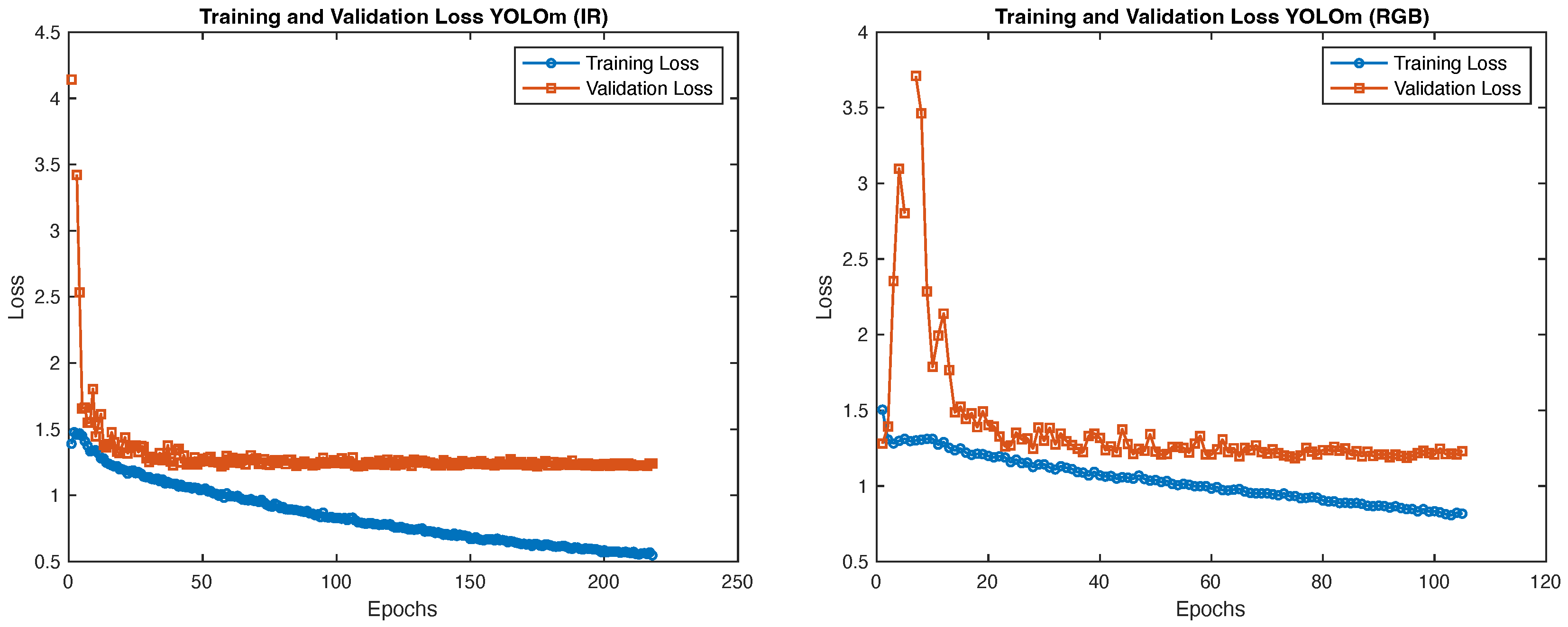
YOLO11 training and validation were performed on a local Ubuntu 24.04 workstation equipped with an AMD Ryzen 5 5600X 6-core CPU and an NVIDIA RTX A6000 GPU (NVIDIA, USA) with 48 GB of VRAM and 64 GB of system RAM. A Python code was used to train different YOLO11 models using the Ultralytics and Roboflow libraries [49,58]. The outcomes of the validation procedure are summarized in Table 5, while Figure 7 illustrates the evolution of training and validation losses across epochs. The curves indicate that there is no noticeable evidence of either overfitting or underfitting during training.

4.3. Multi-Object Tracker and Counting

After testing all YOLO11 variations, YOLO11m obtained the highest F1-score; thus, this model was selected to assess the tracking algorithm. For this purpose, a video showing a segment of a lane from the capsicum greenhouse, containing a known number of capsicums, was used to run the BoT-SORT algorithm. In addition, tests conducted using the IR-based model were also performed using an RGB-based model for comparative analysis. On the other hand, the RGB model selected for these tests is the YOLOm since it outperformed the other versions.
After implementing the BoT-SORT algorithm, an analysis was performed to identify false positives, false negatives, and ID tracking errors, allowing the calculation of the MOTA metric as shown in Equation (10). Finally, the number of capsicums counted by the algorithm and the actual number of capsicums present in the lane are reported to indicate the precision of the counting system.
The results show a low number of ID switches, finding just one through the IR video stream and none in the RGB one; this proves the robustness of the tracker to preserve IDs through frames. Since most of the errors made by the algorithm are false negatives and false positives performed by the detector, the RGB stream presents ten times more false negatives than the IR stream. The results of this analysis are summarized in Table 6.

4.4. Discussion

YOLO11n outperforms the other model variations, achieving a precision of 1 at a confidence rate of 0.96 , as can be seen in Figure 8a, which proves the model’s ability to avoid false positives with high confidence. In addition, the recall-confidence curve shown in Figure 8b presents a 0.92 recall at a confidence level of 0.00 , indicating a high level of identification of true positives through validation. Finally, tests show that the model achieved an F1-score of 0.82 at a confidence level of 0.483 on the F1-score curve (Figure 8c).
The tests performed on the tracker produced a MOTA of 0.85 , indicating that the tracker correctly identified most of the instances that presented few false negatives: 4 out of 70. Also, the system had one single ID track error caused by a capsicum that was correctly identified initially, then occluded for various frames before reappearing in the scene and mistakenly associated with a new track. The fact that the error occurred only once despite several capsicums disappearing due to occlusion and reappearing later proves the BoT-SORT’s ability to identify tracks.
The region counting approach, as mentioned in Section 3.3, enables the system to count capsicums even if they are visible only from a specific angle, yet it is observed that there are capsicums that only appear in a couple of frames, and even when they can be detected by the YOLO11 model, the number of frames is not sufficient to make it into the counting region.
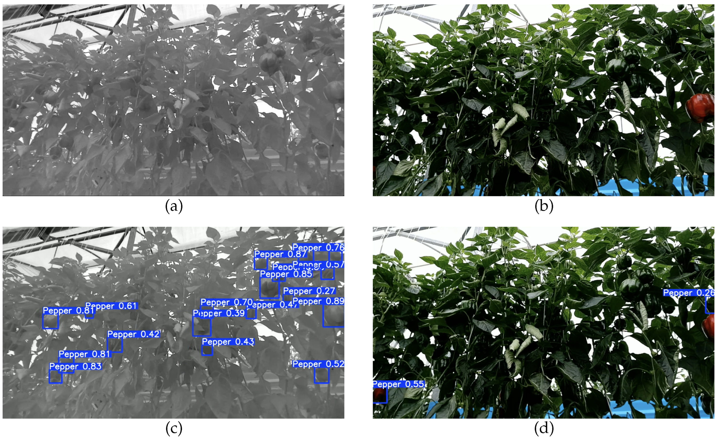
IR offers advantages in detection by highlighting the presence of capsicums among the foliage since they exhibit different intensity at this wavelength. To illustrate this difference, Figure 9 compares IR and RGB images of the same spot in the capsicum lane.
Figure 9b demonstrates the challenging lighting conditions under which the videos were recorded. The capsicums are not directly illuminated and the shadows obscure their visibility. In contrast, Figure 9a presents the IR image of the same spot, captured under identical lighting conditions. Despite the shadows, the capsicums remain visible in the IR wavelength because they contrast sharply with the foliage and background.
This contrast improves detection accuracy, leading to improved recall in predictions using IR images, as shown in Figure 9c, compared to predictions based on RGB images (Figure 9d).
Additionally, the findings further demonstrate the viability of employing IR imagery for capsicum detection and counting. Although prior studies have used IR images primarily to identify defects in other fruit species, no previous work has applied this imaging modality specifically to the detection or counting of capsicums.

5. Conclusions

This work presents a novel capsicum counting algorithm, integrating the state-of-the-art YOLO11 model with the BoT-SORT multi-object tracking algorithm using IR images. The experimental results demonstrate that using IR images allows capsicum detection, even in low-light scenarios. The proposed YOLO11-based detection model achieved an F1-score of 0.82. The multi-object tracking system using BoT-SORT and IR images attained a MOTA of 0.85, further validating the effectiveness of this approach as a capsicum counting application.
A key innovation of this work is the use of IR images instead of the traditional RGB images commonly used in capsicum detection and counting applications. Although multispectral, thermal, and stereo cameras have been explored in previous studies, no prior work has proposed utilizing IR images for this purpose. This approach presents significant advantages in addressing key challenges in fruit counting systems, such as low light conditions caused by shadows and background similarity, without the need for additional hardware, since the camera utilized in this study is integrated into a stereo camera, a widely used device in robotic navigation and agricultural perception applications.
The algorithm developed in this work can count capsicums as long as they are visible at some point by the camera sensor, and it is designed for a greenhouse environment. Partially occluded capsicums and capsicums that appear in the vision range for short instances lead to false negative detections. Therefore, future improvements should focus on developing strategies to mitigate occlusion effects, such as integrating depth information from stereo cameras.
Further research also includes exploring alternative spectral imaging modalities to enhance fruit-background contrast and improve detection robustness. Furthermore, the application of IR imaging techniques should be extended to other fruit types to assess their comparative advantages over RGB-based detection models in different agricultural settings, especially to those with irregular geometry and high similarity to the background scenario. Other future work involves modifying the YOLO architecture to natively process single-channel IR images instead of treating them as three-channel RGB images, potentially optimizing computational efficiency and inference speed. Lastly, future work should integrate depth information with the detection model, since it would not require additional hardware, to assess if it provides useful information to enhance detector performance.

Author Contributions

Conceptualization, E.M. and J.A.E.C.; methodology, E.M. and J.A.E.C.; software, E.M.; validation, E.M.; formal analysis, E.M. and J.A.E.C.; investigation, E.M.; resources, J.A.E.C.; data curation, E.M. and O.O.; writing—original draft preparation, E.M.; writing—review and editing, E.M., J.A.E.C., A.G.-E., J.A.C.-C. and O.O.; visualization, E.M. and O.O.; supervision, J.A.E.C., A.G.-E. and J.A.C.-C.; project administration, J.A.E.C., A.G.-E. and J.A.C.-C.; funding acquisition, J.A.E.C. All authors have read and agreed to the published version of the manuscript.

Funding

This research received no external funding.

Data Availability Statement

The original contributions presented in this study are included in the article material. Further inquiries can be directed to the corresponding author.

Acknowledgments

The authors would like to acknowledge the financial support from SECIHTI for the Ph.D. studies of the first author. We also gratefully acknowledge the support of NVIDIA Corporation through the NVIDIA Academic Grant Program, which provided the GPU resources used in this research.

Conflicts of Interest

The authors declare no conflicts of interest.

References

  1. Ma, L.; Long, H.; Zhang, Y.; Tu, S.; Ge, D.; Tu, X. Agricultural labor changes and agricultural economic development in China and their implications for rural vitalization. J. Geogr. Sci. 2019, 29, 163–179. [Google Scholar] [CrossRef]
  2. Yang, X.; Shu, L.; Chen, J.; Ferrag, M.A.; Wu, J.; Nurellari, E.; Huang, K. A Survey on Smart Agriculture: Development Modes, Technologies, and Security and Privacy Challenges. IEEE/CAA J. Autom. Sin. 2021, 8, 273–302. [Google Scholar] [CrossRef]
  3. Afonso, M.; Fonteijn, H.; Fiorentin, F.S.; Lensink, D.; Mooij, M.; Faber, N.; Polder, G.; Wehrens, R. Tomato Fruit Detection and Counting in Greenhouses Using Deep Learning. Front. Plant Sci. 2020, 11, 571299. [Google Scholar] [CrossRef]
  4. Li, C.; Ma, W.; Liu, F.; Fang, B.; Lu, H.; Sun, Y. Recognition of citrus fruit and planning the robotic picking sequence in orchards. Signal Image Video Process. 2023, 17, 4425–4434. [Google Scholar] [CrossRef]
  5. Montoya-Cavero, L.E.; Díaz de León Torres, R.; Gómez-Espinosa, A.; Escobedo Cabello, J.A. Vision systems for harvesting robots: Produce detection and localization. Comput. Electron. Agric. 2022, 192, 106562. [Google Scholar] [CrossRef]
  6. Maktab Dar Oghaz, M.; Razaak, M.; Kerdegari, H.; Argyriou, V.; Remagnino, P. Scene and Environment Monitoring Using Aerial Imagery and Deep Learning. In Proceedings of the 2019 15th International Conference on Distributed Computing in Sensor Systems (DCOSS), Santorini Island, Greece, 29–31 May 2019; pp. 362–369. [Google Scholar] [CrossRef]
  7. Osman, Y.; Dennis, R.; Elgazzar, K. Yield Estimation and Visualization Solution for Precision Agriculture. Sensors 2021, 21, 6657. [Google Scholar] [CrossRef]
  8. Huang, S.C.; Le, T.H. Chapter 12—Object detection. In Principles and Labs for Deep Learning; Huang, S.C., Le, T.H., Eds.; Academic Press: Cambridge, MA, USA, 2021; pp. 283–331. [Google Scholar] [CrossRef]
  9. Hou, G.; Chen, H.; Jiang, M.; Niu, R. An Overview of the Application of Machine Vision in Recognition and Localization of Fruit and Vegetable Harvesting Robots. Agriculture 2023, 13, 1814. [Google Scholar] [CrossRef]
  10. Lin, G.; Tang, Y.; Zou, X.; Xiong, J.; Fang, Y. Color-, depth-, and shape-based 3D fruit detection. Precis. Agric. 2020, 21, 1–17. [Google Scholar] [CrossRef]
  11. Akbar, J.U.M.; Kamarulzaman, S.F.; Muzahid, A.J.M.; Rahman, M.A.; Uddin, M. A Comprehensive Review on Deep Learning Assisted Computer Vision Techniques for Smart Greenhouse Agriculture. IEEE Access 2024, 12, 4485–4522. [Google Scholar] [CrossRef]
  12. Paul, A.; Machavaram, R.; Ambuj; Kumar, D.; Nagar, H. Smart solutions for capsicum Harvesting: Unleashing the power of YOLO for Detection, Segmentation, growth stage Classification, Counting, and real-time mobile identification. Comput. Electron. Agric. 2024, 219, 108832. [Google Scholar] [CrossRef]
  13. Jiang, Y.; Li, C. Convolutional Neural Networks for Image-Based High-Throughput Plant Phenotyping: A Review. Plant Phenomics 2020, 2020, 4152816. [Google Scholar] [CrossRef] [PubMed]
  14. Krizhevsky, A.; Sutskever, I.; Hinton, G.E. ImageNet Classification with Deep Convolutional Neural Networks. In Proceedings of the Advances in Neural Information Processing Systems; Curran Associates, Inc.: New York, NY, USA, 2012; Volume 25. [Google Scholar]
  15. Espinoza, S.; Aguilera, C.; Rojas, L.; Campos, P.G. Analysis of Fruit Images With Deep Learning: A Systematic Literature Review and Future Directions. IEEE Access 2024, 12, 3837–3859. [Google Scholar] [CrossRef]
  16. Girshick, R.; Donahue, J.; Darrell, T.; Malik, J. Rich Feature Hierarchies for Accurate Object Detection and Semantic Segmentation. In Proceedings of the 2014 IEEE Conference on Computer Vision and Pattern Recognition, Columbus, OH, USA, 23–28 June 2014; pp. 580–587, ISSN 1063-6919. [Google Scholar] [CrossRef]
  17. Redmon, J.; Divvala, S.; Girshick, R.; Farhadi, A. You Only Look Once: Unified, Real-Time Object Detection. In Proceedings of the 2016 IEEE Conference on Computer Vision and Pattern Recognition (CVPR), Las Vegas, NV, USA, 27–30 June 2016; pp. 779–788, ISSN 1063-6919. [Google Scholar] [CrossRef]
  18. He, K.; Gkioxari, G.; Dollar, P.; Girshick, R. Mask R-CNN. In Proceedings of the 2017 IEEE International Conference on Computer Vision (ICCV), Venice, Italy, 22–29 October 2017; pp. 2980–2988. [Google Scholar] [CrossRef]
  19. Tu, S.; Pang, J.; Liu, H.; Zhuang, N.; Chen, Y.; Zheng, C.; Wan, H.; Xue, Y. Passion fruit detection and counting based on multiple scale faster R-CNN using RGB-D images. Precis. Agric. 2020, 21, 1072–1091. [Google Scholar] [CrossRef]
  20. Behera, S.K.; Rath, A.K.; Sethy, P.K. Fruits yield estimation using Faster R-CNN with MIoU. Multimed. Tools Appl. 2021, 80, 19043–19056. [Google Scholar] [CrossRef]
  21. Assunção, E.T.; Gaspar, P.D.; Mesquita, R.J.M.; Simões, M.P.; Ramos, A.; Proença, H.; Inacio, P.R.M. Peaches Detection Using a Deep Learning Technique—A Contribution to Yield Estimation, Resources Management, and Circular Economy. Climate 2022, 10, 11. [Google Scholar] [CrossRef]
  22. Sapkota, R.; Ahmed, D.; Karkee, M. Comparing YOLOv8 and Mask R-CNN for instance segmentation in complex orchard environments. Artif. Intell. Agric. 2024, 13, 84–99. [Google Scholar] [CrossRef]
  23. Badgujar, C.M.; Poulose, A.; Gan, H. Agricultural object detection with You Only Look Once (YOLO) Algorithm: A bibliometric and systematic literature review. Comput. Electron. Agric. 2024, 223, 109090. [Google Scholar] [CrossRef]
  24. Bazame, H.C.; Molin, J.P.; Althoff, D.; Martello, M. Detection, classification, and mapping of coffee fruits during harvest with computer vision. Comput. Electron. Agric. 2021, 183, 106066. [Google Scholar] [CrossRef]
  25. Chen, W.; Zhang, J.; Guo, B.; Wei, Q.; Zhu, Z. An Apple Detection Method Based on Des-YOLO v4 Algorithm for Harvesting Robots in Complex Environment. Math. Probl. Eng. 2021, 2021, 7351470. [Google Scholar] [CrossRef]
  26. Mirhaji, H.; Soleymani, M.; Asakereh, A.; Abdanan Mehdizadeh, S. Fruit detection and load estimation of an orange orchard using the YOLO models through simple approaches in different imaging and illumination conditions. Comput. Electron. Agric. 2021, 191, 106533. [Google Scholar] [CrossRef]
  27. Gai, R.; Chen, N.; Yuan, H. A detection algorithm for cherry fruits based on the improved YOLO-v4 model. Neural Comput. Appl. 2023, 35, 13895–13906. [Google Scholar] [CrossRef]
  28. Tsai, F.T.; Nguyen, V.T.; Duong, T.P.; Phan, Q.H.; Lien, C.H. Tomato Fruit Detection Using Modified Yolov5m Model with Convolutional Neural Networks. Plants 2023, 12, 3067. [Google Scholar] [CrossRef] [PubMed]
  29. Du, X.; Cheng, H.; Ma, Z.; Lu, W.; Wang, M.; Meng, Z.; Jiang, C.; Hong, F. DSW-YOLO: A detection method for ground-planted strawberry fruits under different occlusion levels. Comput. Electron. Agric. 2023, 214, 108304. [Google Scholar] [CrossRef]
  30. Giacomin, R.; Constantino, L.; Nogueira, A.; Ruzza, M.; Morelli, A.; Branco, K.; Rossetto, L.; Zeffa, D.; Gonçalves, L. Post-harvest quality and sensory evaluation of mini sweet peppers. Horticulturae 2021, 7, 287. [Google Scholar] [CrossRef]
  31. Zou, X.; Ma, Y.; Dai, X.; Li, X.; Yang, S. Spread and Industry Development of Pepper in China. Acta Hortic. Sin. 2020, 47, 1715. [Google Scholar] [CrossRef]
  32. Cong, P.; Li, S.; Zhou, J.; Lv, K.; Feng, H. Research on Instance Segmentation Algorithm of Greenhouse Sweet Pepper Detection Based on Improved Mask RCNN. Agronomy 2023, 13, 196. [Google Scholar] [CrossRef]
  33. López-Barrios, J.D.; Escobedo Cabello, J.A.; Gómez-Espinosa, A.; Montoya-Cavero, L.E. Green Sweet Pepper Fruit and Peduncle Detection Using Mask R-CNN in Greenhouses. Appl. Sci. 2023, 13, 6296. [Google Scholar] [CrossRef]
  34. Viveros Escamilla, L.D.; Gómez-Espinosa, A.; Escobedo Cabello, J.A.; Cantoral-Ceballos, J.A. Maturity Recognition and Fruit Counting for Sweet Peppers in Greenhouses Using Deep Learning Neural Networks. Agriculture 2024, 14, 331. [Google Scholar] [CrossRef]
  35. Wojke, N.; Bewley, A.; Paulus, D. Simple online and realtime tracking with a deep association metric. In Proceedings of the 2017 IEEE International Conference on Image Processing (ICIP), Beijing, China, 17–20 September 2017; pp. 3645–3649, ISSN 2381-8549. [Google Scholar] [CrossRef]
  36. Zhang, X.; Zhu, D.; Wen, R. SwinT-YOLO: Detection of densely distributed maize tassels in remote sensing images. Comput. Electron. Agric. 2023, 210, 107905. [Google Scholar] [CrossRef]
  37. Feng, J.; Zeng, L.; He, L. Apple Fruit Recognition Algorithm Based on Multi-Spectral Dynamic Image Analysis. Sensors 2019, 19, 949. [Google Scholar] [CrossRef]
  38. Wu, X.; Wu, X.; Huang, H.; Zhang, F.; Wen, Y. Characterization of Pepper Ripeness in the Field Using Hyperspectral Imaging (HSI) with Back Propagation (BP) Neural Network and Kernel Based Extreme Learning Machine (KELM) Models. Anal. Lett. 2024, 57, 409–424. [Google Scholar] [CrossRef]
  39. Zhang, H.; Zhang, S.; Dong, W.; Luo, W.; Huang, Y.; Zhan, B.; Liu, X. Detection of common defects on mandarins by using visible and near infrared hyperspectral imaging. Infrared Phys. Technol. 2020, 108, 103341. [Google Scholar] [CrossRef]
  40. Gan, H.; Lee, W.S.; Alchanatis, V.; Abd-Elrahman, A. Active thermal imaging for immature citrus fruit detection. Biosyst. Eng. 2020, 198, 291–303. [Google Scholar] [CrossRef]
  41. Paul, A.; Machavaram, R. Greenhouse capsicum detection in thermal imaging: A comparative analysis of a single-shot and a novel zero-shot detector. Next Res. 2024, 1, 100076. [Google Scholar] [CrossRef]
  42. Tsuchikawa, S.; Ma, T.; Inagaki, T. Application of near-infrared spectroscopy to agriculture and forestry. Anal. Sci. 2022, 38, 635–642. [Google Scholar] [CrossRef]
  43. Patel, K.K.; Pathare, P.B. Principle and applications of near-infrared imaging for fruit quality assessment—An overview. Int. J. Food Sci. Technol. 2024, 59, 3436–3450. [Google Scholar] [CrossRef]
  44. Fan, S.; Liang, X.; Huang, W.; Jialong Zhang, V.; Pang, Q.; He, X.; Li, L.; Zhang, C. Real-time defects detection for apple sorting using NIR cameras with pruning-based YOLOV4 network. Comput. Electron. Agric. 2022, 193, 106715. [Google Scholar] [CrossRef]
  45. Fan, S.; Li, C.; Huang, W.; Chen, L. Detection of blueberry internal bruising over time using NIR hyperspectral reflectance imaging with optimum wavelengths. Postharvest Biol. Technol. 2017, 134, 55–66. [Google Scholar] [CrossRef]
  46. Wang, C.; Liu, S.; Wang, Y.; Xiong, J.; Zhang, Z.; Zhao, B.; Luo, L.; Lin, G.; He, P. Application of Convolutional Neural Network-Based Detection Methods in Fresh Fruit Production: A Comprehensive Review. Front. Plant Sci. 2022, 13, 868745. [Google Scholar] [CrossRef] [PubMed]
  47. Jiang, P.; Ergu, D.; Liu, F.; Cai, Y.; Ma, B. A Review of Yolo Algorithm Developments. Procedia Comput. Sci. 2022, 199, 1066–1073. [Google Scholar] [CrossRef]
  48. Terven, J.; Córdova-Esparza, D.M.; Romero-González, J.A. A Comprehensive Review of YOLO Architectures in Computer Vision: From YOLOv1 to YOLOv8 and YOLO-NAS. Mach. Learn. Knowl. Extr. 2023, 5, 1680–1716. [Google Scholar] [CrossRef]
  49. Jocher, G.; Qiu, J.; Chaurasia, A. Ultralytics YOLO (Version 8.0.0) [Computer software]. Available online: https://github.com/ultralytics/ultralytics (accessed on 18 November 2025).
  50. Huang, J.; Wang, K.; Hou, Y.; Wang, J. LW-YOLO11: A Lightweight Arbitrary-Oriented Ship Detection Method Based on Improved YOLO11. Sensors 2025, 25, 65. [Google Scholar] [CrossRef]
  51. Khanam, R.; Hussain, M. YOLOv11: An Overview of the Key Architectural Enhancements. arXiv 2024, arXiv:2410.17725. [Google Scholar] [CrossRef]
  52. Zhang, Y.; Sun, P.; Jiang, Y.; Yu, D.; Weng, F.; Yuan, Z.; Luo, P.; Liu, W.; Wang, X. ByteTrack: Multi-Object Tracking by Associating Every Detection Box. arXiv 2022, arXiv:2110.06864. [Google Scholar] [CrossRef]
  53. Aharon, N.; Orfaig, R.; Bobrovsky, B.Z. BoT-SORT: Robust Associations Multi-Pedestrian Tracking. arXiv 2022, arXiv:2206.14651. [Google Scholar] [CrossRef]
  54. Siriani, A.L.R.; Miranda, I.B.D.C.; Mehdizadeh, S.A.; Pereira, D.F. Chicken Tracking and Individual Bird Activity Monitoring Using the BoT-SORT Algorithm. AgriEngineering 2023, 5, 1677–1693. [Google Scholar] [CrossRef]
  55. Yang, X.; Gao, Y.; Yin, M.; Li, H. Automatic Apple Detection and Counting with AD-YOLO and MR-SORT. Sensors 2024, 24, 7012. [Google Scholar] [CrossRef]
  56. He, K.; Zhang, X.; Ren, S.; Sun, J. Deep Residual Learning for Image Recognition. In Proceedings of the 2016 IEEE Conference on Computer Vision and Pattern Recognition (CVPR), Las Vegas, NV, USA, 27–30 June 2016; pp. 770–778. [Google Scholar] [CrossRef]
  57. Kuhn, H.W. The Hungarian method for the assignment problem. Nav. Res. Logist. Q. 1955, 2, 83–97. [Google Scholar] [CrossRef]
  58. Dwyer, B.; Nelson, J.; Hansen, T. Roboflow (Version 1.0) [Software]. Computer Vision Software. 2025. Available online: https://roboflow.com (accessed on 18 November 2025).
  59. Mendez, E. Capsicum IR Box Annotation Computer Vision Dataset. 1000 Images with 11,916 Labeled Instances. 2025. Available online: https://universe.roboflow.com/enrico-mendez-research-s9yeb/capsicum-ir-box (accessed on 18 November 2025).
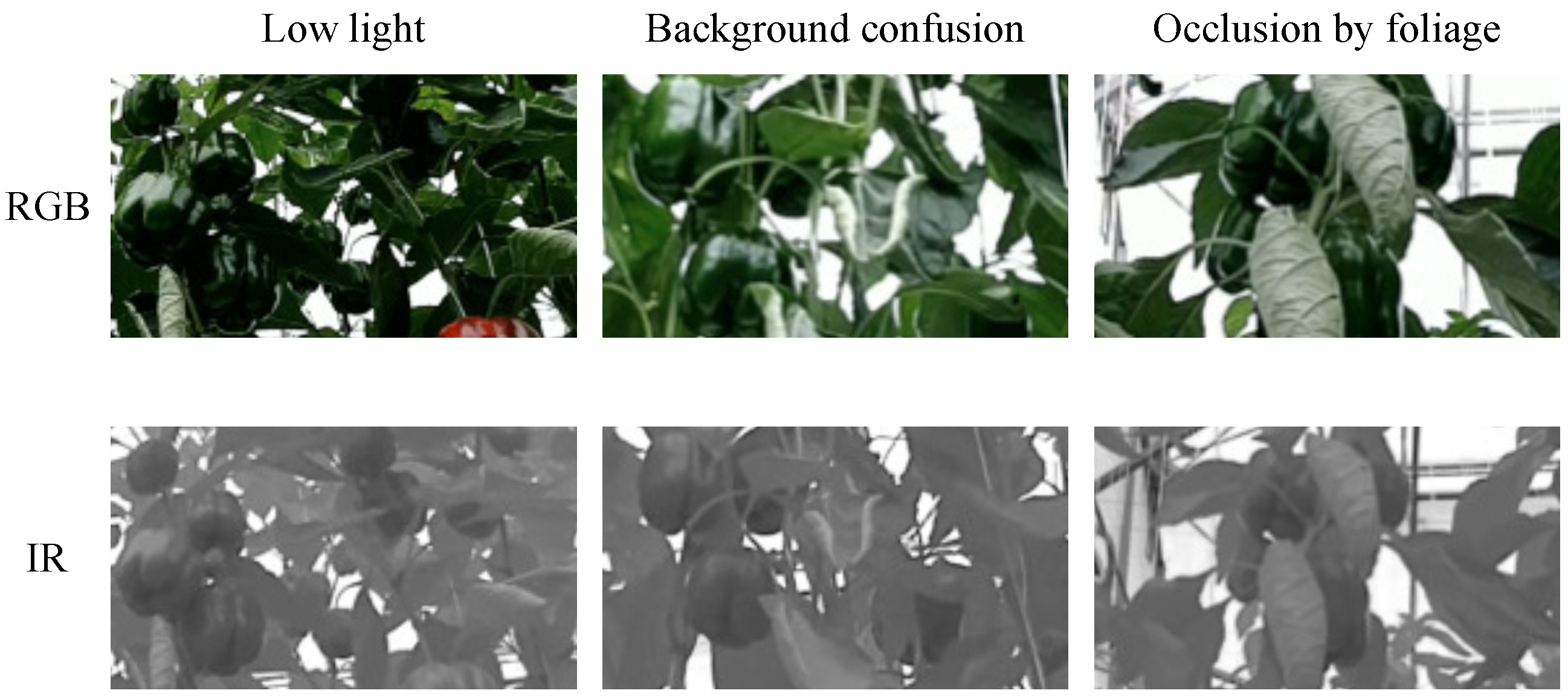
Figure 1. Main challenges in capsicum counting applications seen in RGB and IR images.
Agriculture 15 02574 g001
Figure 3. Workflow of the BoT-SORT pipeline. The detection stage uses YOLO11 to obtain bounding boxes (black), the prediction stage uses a Kalman filter to estimate future positions (green), data association is resolved by the Hungarian algorithm (red), and finally, track updates link detections with previously tracked objects (blue) [53].
Agriculture 15 02574 g003
Figure 4. (a) The mobile robotic platform setup comprises a camera mounted on a gimbal for image acquisition. (b) The mobile robotic platform operates in a capsicum greenhouse for data collection.
Agriculture 15 02574 g004
Figure 5. RGB, grayscale, and IR images and the result after applying contrast where α = 2 and β = 0 .
Agriculture 15 02574 g005
Figure 6. Example of the counter code output, the counting region delineated by a purple rectangle, extending from 0.33 to 0.75 of the frame width. The blue squares indicate current detections and the blue lines represent the tracks associated with a detection.
Agriculture 15 02574 g006
Figure 7. Evolution of training and validation losses across epochs for the YOLO11m with the IR dataset (left) and for the YOLOm with the RGB dataset (right).
Agriculture 15 02574 g007
Figure 8. YOLO 11m validation metrics plots. (a) Precision-Confidence curve plot. (b) Recall-Confidence curve plot. (c) F1-score curve plot.
Agriculture 15 02574 g008
Figure 9. Examples of images taken with different sensors and their corresponding predictions. (a) IR image, where capsicums remain clearly visible even in low-light regions and under occlusion. (b) RGB image of the same scene, where capsicums are less visible in dark regions due to lighting conditions. (c) Predicted bounding boxes on the IR image. (d) Predicted bounding boxes on the RGB image.
Agriculture 15 02574 g009
Table 2. Tracking Algorithm Parameters.
ParameterDescriptionValue
track_high_threshThreshold for the first association0.5
track_low_threshThreshold for the second association0.3
new_track_threshThreshold for initializing a new track if no match is found0.29
track_bufferBuffer to determine when to remove tracks35
match_threshThreshold for matching tracks0.8
Table 3. Data-augmentation hyperparameters enabled during YOLO training in the Ultralytics framework.
Augmentation (argument)DescriptionValue
Hue shift ( h s v _ h )Random perturbation of image hue in HSV space0.015 (maximum hue offset)
Saturation shift ( h s v _ s )Random perturbation of color saturation0.70 (maximum relative change in saturation)
Brightness shift ( h s v _ v )Random perturbation of brightness0.40 (maximum relative change in brightness)
Translation ( t r a n s l a t e )Random x/y translation0.10 (maximum fraction of image size used for shifting)
Scale ( s c a l e )Random zoom in/out0.50 (maximum relative scaling factor)
Horizontal flip ( f l i p l r )Left–right flip0.50 (probability of flipping eachtraining image)
Mosaic ( m o s a i c )Combines four training images into a single mosaic image1.0 (probability of applying mosaic)
Table 4. YOLO11 training configuration parameters.
ParameterDescriptionValue
epochsNumber of training iterations over the entire dataset.500
batchSize of the batch for training, with 0.9 indicating the code to calculate the batch size to use 90% of the GPU memory.64
imgszThe size of the input images during training, resized to this size for processing.800
cacheHow the dataset is loaded into memory for training. ram indicates that the dataset is cached in RAM.ram
optimizerOptimization algorithm used to update the model weights during training.Adam
patienceEarly stopping parameter, specifying the number of epochs to wait, if improvement has not been observed, before stopping.100
Table 5. Performance Metrics for YOLO11 Models.
ModelRecall (Best)Precision (Best)F1-Score (Best)Dataset
YOLO11n0.8810.81IR
YOLO11s0.9610.81IR
YOLO11m0.9210.82IR
YOLO11n0.9210.82RGB
YOLO11s0.9510.81RGB
YOLO11m0.9310.82RGB
Table 6. Multiple object tracker accuracy per sensor.
SensorGround TruthCounted CapsicumsFPFNIDSMOTA
IR70675410.85
RGB702534300.34
Disclaimer/Publisher’s Note: The statements, opinions and data contained in all publications are solely those of the individual author(s) and contributor(s) and not of MDPI and/or the editor(s). MDPI and/or the editor(s) disclaim responsibility for any injury to people or property resulting from any ideas, methods, instructions or products referred to in the content.