Study on the Impact of Grazing Density on Seasonal Pasture NPP in the Northern Slope of the Tianshan Mountains in Xinjiang: A Case Study of Hutubi County

Abstract

Grazing pressure (GP) was a key factor influencing net primary productivity (NPP) in pasturelands and was characterized by two indicators: grazing intensity (GI) and grazing density (GD). However, current research has not yet clarified whether the mechanisms linking GP to NPP varied by season, or whether seasonal thresholds of grazing pressure existed. This study employed the Carnegie–Ames–Stanford Approach (CASA) model to estimate NPP over eight time periods between 2010 and 2024 for three seasonal pastures (spring–autumn, summer, and winter) in the study area. Estimation accuracy was evaluated by comparing our NPP estimates with existing NPP products. Trends in NPP and their significance were analyzed using the Sen–MK method, followed by further examination of spatiotemporal variations in NPP across the three seasonal pastures. Subsequently, by comparing two grazing pressure indicators (GI and GD), we identified the optimal metric to represent GP and, on this basis, analyzed the spatiotemporal variations and threshold dynamics of pasture NPP across three seasons under the influence of GP. Results indicated that the CASA model achieved R² > 0.90 for multi-year NPP estimation, with RMSE ranging from 27 to 45 g C m⁻² y⁻¹. Spring–autumn and winter pastures exhibited pronounced slope changes and intense spatiotemporal NPP variations, whereas summer pastures showed insignificant slope changes and stable spatiotemporal NPP patterns. Of the two GP indicators, the GD metric developed herein more effectively characterized grazing pressure across the study area. Across the three seasonal pastures, a consistent negative feedback between GD and NPP was evident; however, its strength differed markedly, with spring–autumn and winter pastures exhibiting greater NPP sensitivity to GD. The GD thresholds for spring–autumn, summer, and winter pastures in the study area were approximately 900, 700, and 5000 sheep km⁻², respectively. Exceeding these thresholds led to degradation, while falling below them promoted recovery. The study revealed a threshold-mediated negative feedback between GD and NPP across seasonal pastures, quantified season-specific upper bounds of carrying capacity, and provided an evidence base for zoned rest/rotational grazing and GD regulation along the northern slope of the Tianshan Mountains.

1. Introduction

NPP is the organic matter accumulated by plants via photosynthesis after subtracting their autotrophic respiration [1]. As a key indicator for assessing ecosystem health, NPP not only quantifies the net increase in organic matter accumulated by plants through photosynthesis but also reveals the dynamic equilibrium of grassland carbon storage capacity, nutrient cycling, and biodiversity maintenance [2]. Currently, with the intensification of factors such as climate variability, soil erosion, and human disturbance, grasslands in many regions face the risk of degradation. Among these factors, human disturbance plays a significant role, primarily manifested as overgrazing. Overgrazing reduces grassland aboveground net primary productivity (ANPP) through livestock consumption and decreases grassland belowground net primary productivity (BNPP) through trampling, thereby diminishing grassland NPP and exacerbating the risk of grassland degradation [3]. Accordingly, elucidating how GP affects grassland NPP—and the mechanisms involved—is essential for restoring grassland ecosystem services and securing the long-term sustainability of pastoral livestock systems. Moreover, while existing work has largely focused on the effects of GP on soil erosion, plant community traits, and soil physicochemical properties, the specific mechanisms by which GP drives changes in NPP remain underexplored, leaving a critical gap to be addressed [4,5,6].

Grassland NPP estimation can be broadly categorized into non-remote sensing methods and remote sensing methods. Non-remote sensing methods include the following: direct measurement methods [7], ecosystem process models (e.g., TEM, BIOME-BGC, and CENTURY) [8,9,10], and empirical statistical models (e.g., Miami, Thornthwaite, and Chikugo) [11,12,13]. Although these methods offer high accuracy, they involve significant upfront costs and are limited to small-scale NPP estimation. In contrast, remote sensing methods, driven by satellite observations and meteorological data, enable large-scale spatiotemporal distribution inversion of NPP. Key approaches include light-use efficiency (LUE) models (e.g., CASA, MOD17, GLO-PEM, and VPM) [14,15,16], SIF-constrained methods [17], and machine learning upsampling (FLUXCOM approach) [18]. Among these, SIF-constrained methods are sensitive to stress responses but suffer from resolution and inversion uncertainties. Machine learning upscaling methods use tower flux measurements as ground truth, integrating remote sensing and meteorological data to train models capable of generating multi-year global products. However, interpolation analysis may introduce bias in trend interpretations. LUE models, calculated through photosynthetically active radiation (PAR) and photosynthetic efficiency (ε), exhibit robust data requirements and high interpretability. They are most widely applied in arid/semi-arid grasslands, with the CASA model being the most extensively used and well-validated. Current CASA model variants include the standard version [19,20], MODIS-driven version [15], and regionally optimized version [21]. This study adopts the regionally optimized CASA model as the primary method due to its parameter optimization for China’s arid grasslands and extensive regional-scale validation, making it more suitable for the study area’s characteristics.

GP is a key indicator of the anthropogenic disturbance imposed on grassland ecosystems; in practice, many studies use GI to characterize the GP exerted on a given area over a specified period. It can be defined as the cumulative impact exerted by grazing animals on a pasture over a specified period or, equivalently, as the ratio of herbage removed to herbage available during that period [22,23]. Formally, under the NZSAP framework (Occasional Publication No. 10), GI is operationalized as herbage removed relative to herbage availability [24]. Many scholars have explored how to use GI to represent GP. For example, Wang et al. [25] combined county-level livestock census data with satellite-derived grassland biomass differences to produce a long-term GI dataset, providing an important reference for identifying the impacts of grazing activities on grassland dynamics. However, such remote-sensing inversion approaches [26,27] typically construct GI from vegetation metrics within a given time window (e.g., LAI ratios or NDVI differences; see Section 3.2). 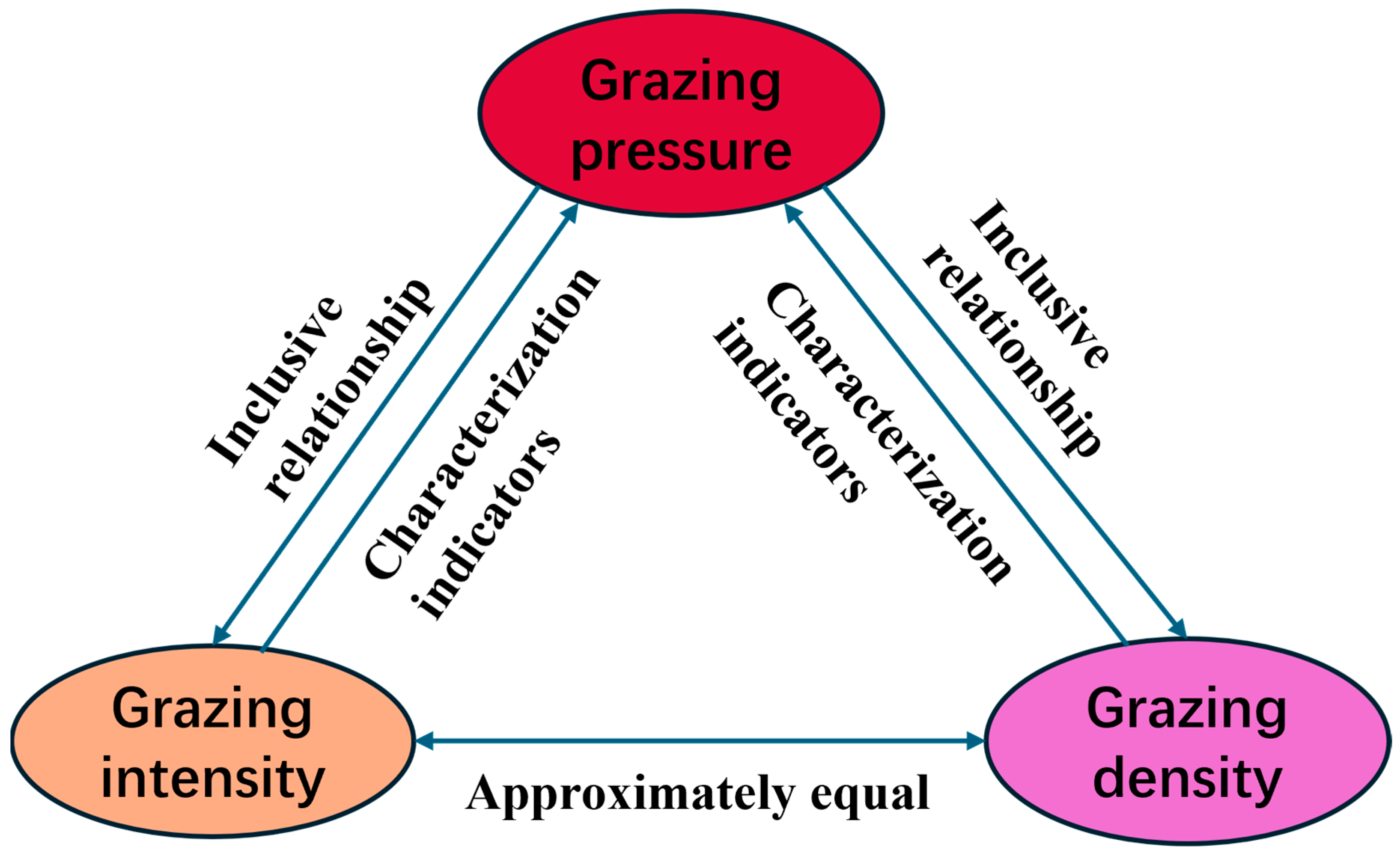Consequently, GI is strongly collinear with NPP itself [28], which can obscure the negative feedback of GP on NPP. By contrast, GD—estimated from livestock inventories and pasture area—more faithfully reflects actual GP [29] (see Appendix D.6 for the GP–GD–GI schema). Mechanistically, GD captures the negative GP–NPP linkage because GP acts through the light-use efficiency (ε) pathway in productivity models: classic grazing studies show ε is a function of GI (Lemaire et al., 2000, Table 18.7 [30]). Hence, higher stocking pressure depresses ε—and thus NPP—particularly under moisture- or temperature-limited conditions. This process view also clarifies why climate and policy matter: precipitation/temperature anomalies and rest/rotational-grazing policies jointly modulate ε and realized APAR, reshaping GP’s net effect on NPP. Practically, compared with GI products derived from remote sensing or in situ measurements, a GD-based metric is easier to obtain and process and avoids reliance on vegetation indices. Accordingly, we adopt a GD-grounded GP metric and investigate how GD drives NPP dynamics.

Focusing on the GP–NPP relationship, prior studies have highlighted a negative feedback between GP and NPP, as well as the stimulatory effect of light GP on NPP. For example, Irisarri et al. [31] found that light increases in GP decreased C₃ grass biomass while increasing C₄ grass biomass. Likewise, Chi et al. [32] reported a significant negative correlation between NPP residuals and GP. Cui [33] noted that moderate grazing is conducive to maintaining species diversity and community structure. 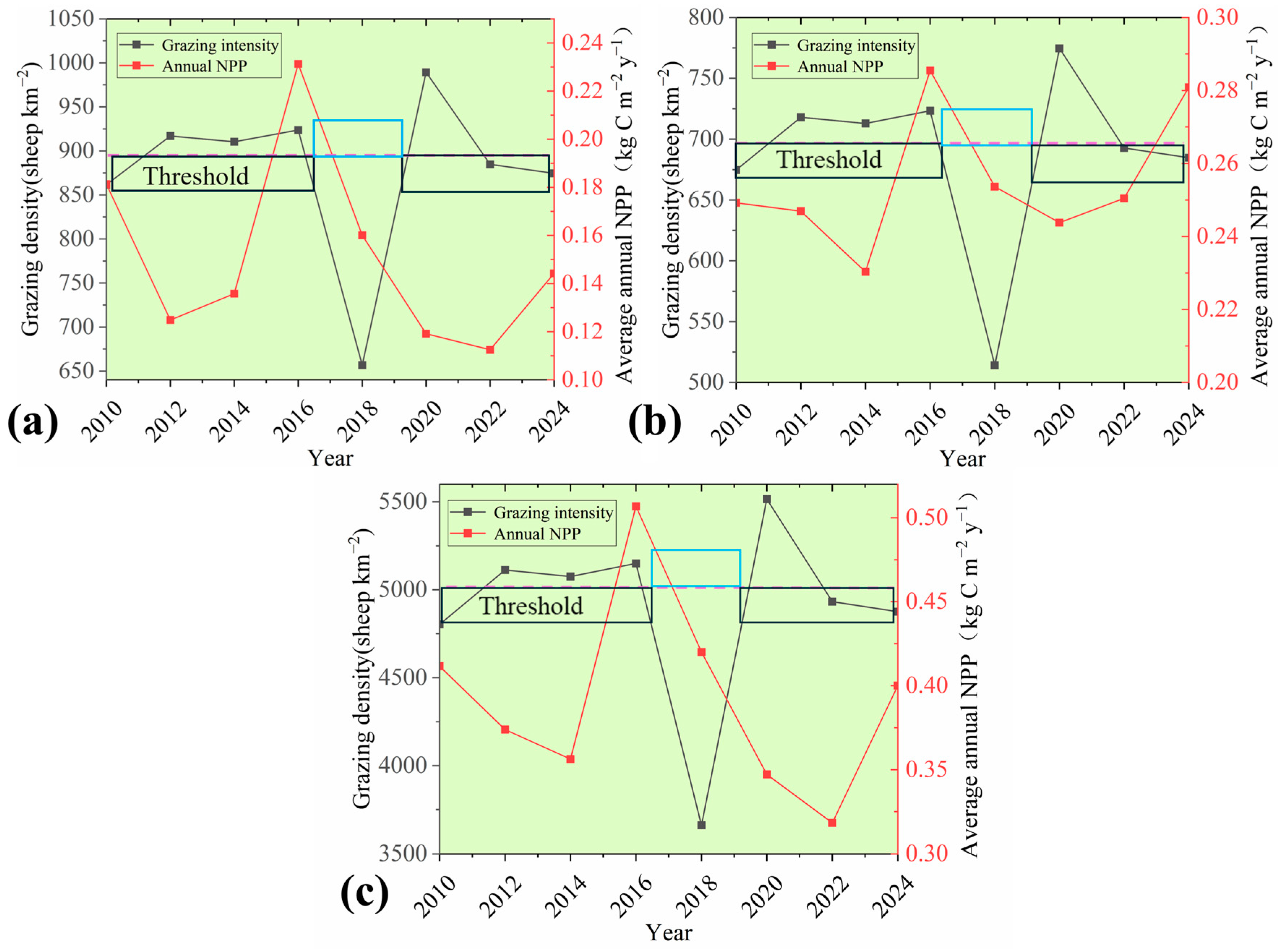In addition, Hou [34] examined the effects of GP on NPP in dry versus wet years and found that NPP follows a quadratic relationship with GP in dry years (peaking under light grazing), but declines linearly in wet years—consistent with the grazing-avoidance hypothesis. However, the above studies treated all pastures within a region as a single unit and averaged the effects of GP on NPP; this overlooks the distinctions among seasonal pastures (spring–autumn, summer, winter) and thus fails to capture season-specific GP–NPP relationships. Accordingly, a key challenge is to efficiently and quantitatively assess how GP—operationalized here as GD—affects NPP across different seasonal pastures, and to systematically compare seasonal differences in NPP responses to GP (e.g., thresholds and shifts in NPP levels). This is a central problem in GP–NPP research and the core focus of the present study.

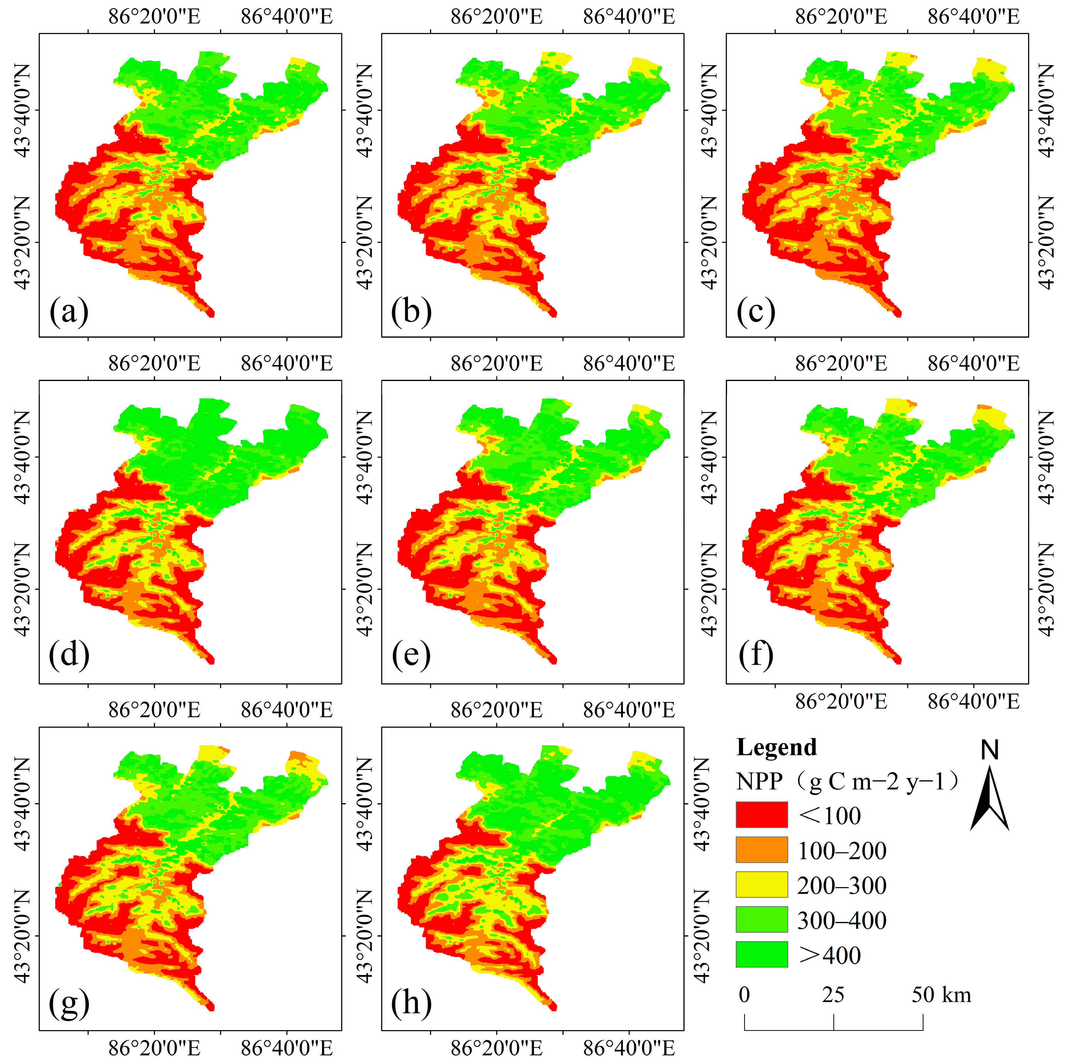
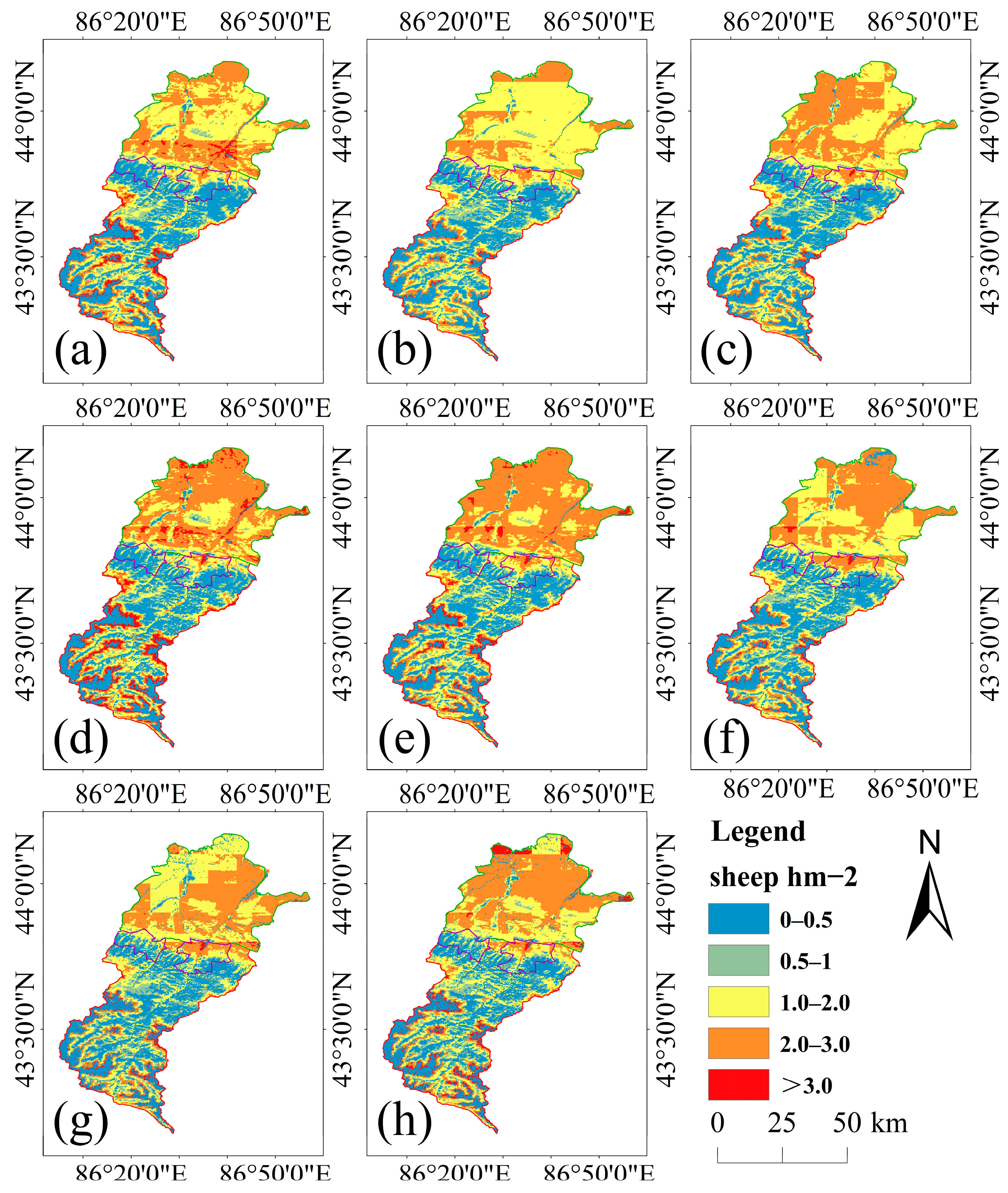
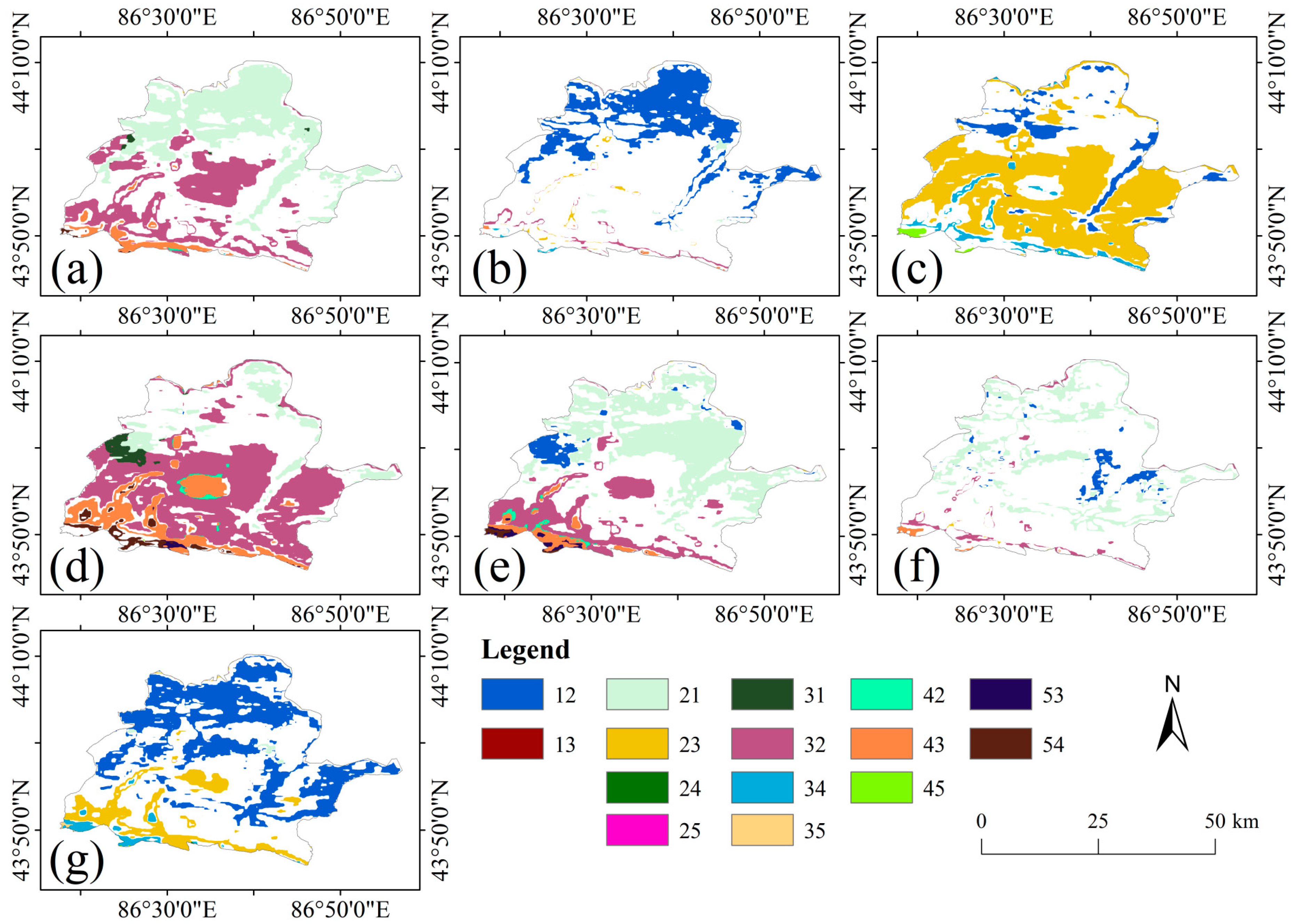
To investigate how GP influences NPP across seasonal pastures and to characterize associated threshold dynamics—while identifying the most accurate indicator of GP—we proceed as follows. First, we retrieve seasonal-pasture NPP using the CASA model and detect multi-year NPP trends with the Sen’s slope–Mann–Kendall (Sen–MK) approach. Second, by comparing an existing GI product with our GD dataset, we select the indicator that best represents actual GP and, using a transition-matrix analysis, quantify GD-driven shifts in NPP classes across seasons. Finally, we synthesize the threshold ranges and general regularities for different seasonal pastures to provide operational, quantitative guidance for zoned rest grazing, rotational grazing, and intensity regulation in arid and semi-arid regions.

2. Methods

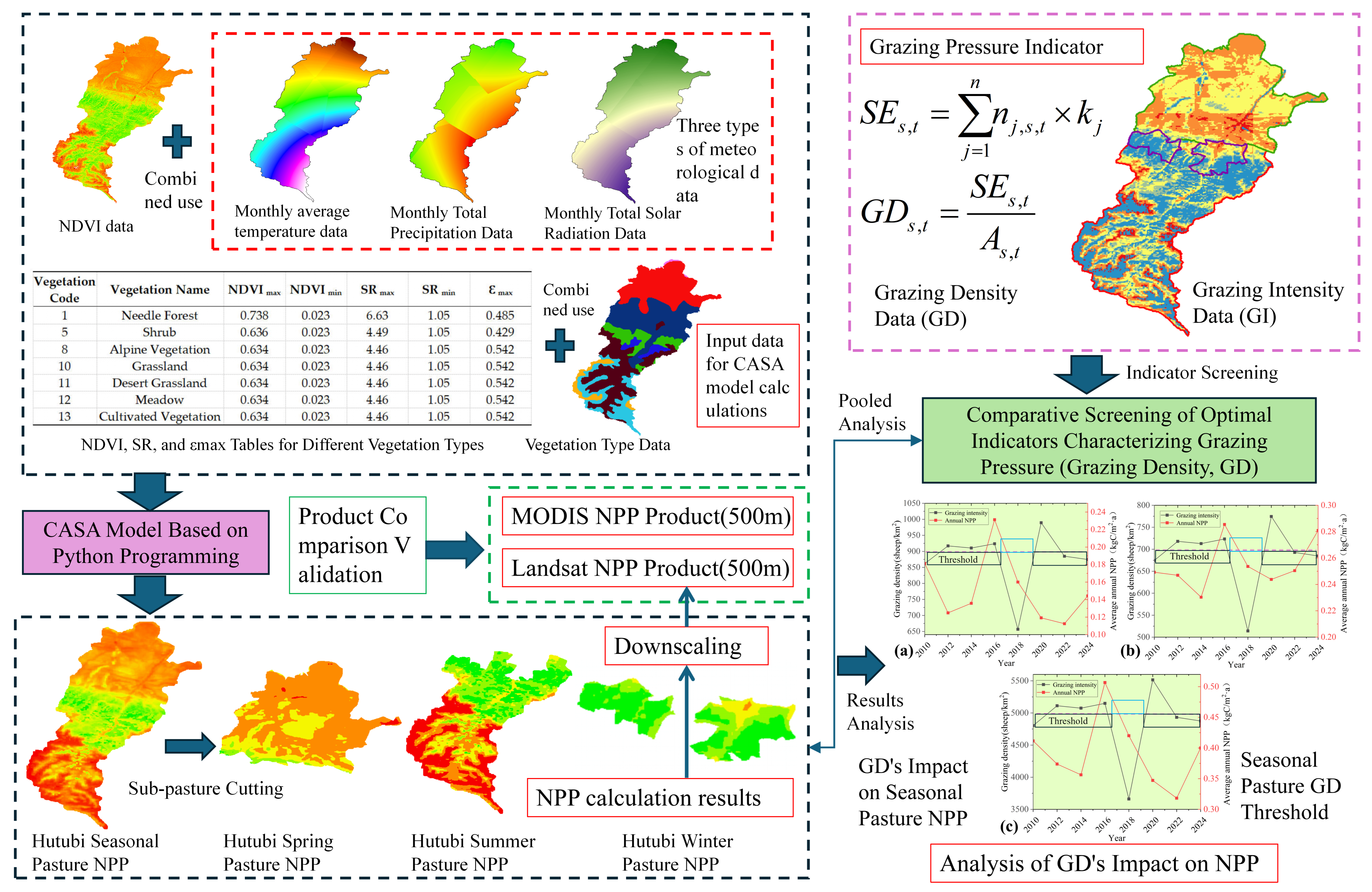
The technical workflow (Figure 1) comprised four steps: (1) Data acquisition: We collected NDVI; meteorological variables (monthly mean air temperature, monthly total precipitation, and monthly total solar radiation); vegetation type data (both raster and tabular; see Appendix D.4); and grazing pressure data (GD and GI). (2) Model development: We implemented the CASA light-use efficiency model in Python (version: 3.8.20) to estimate NPP. (3) Model validation: We evaluated model reliability by comparing our NPP estimates against the MODIS NPP product and by conducting trend analyses on the estimated NPP. (4) Result analysis: We analyzed GD-driven spatiotemporal variations in NPP to provide scientific support for grassland management and policy making.

2.1. Study Area

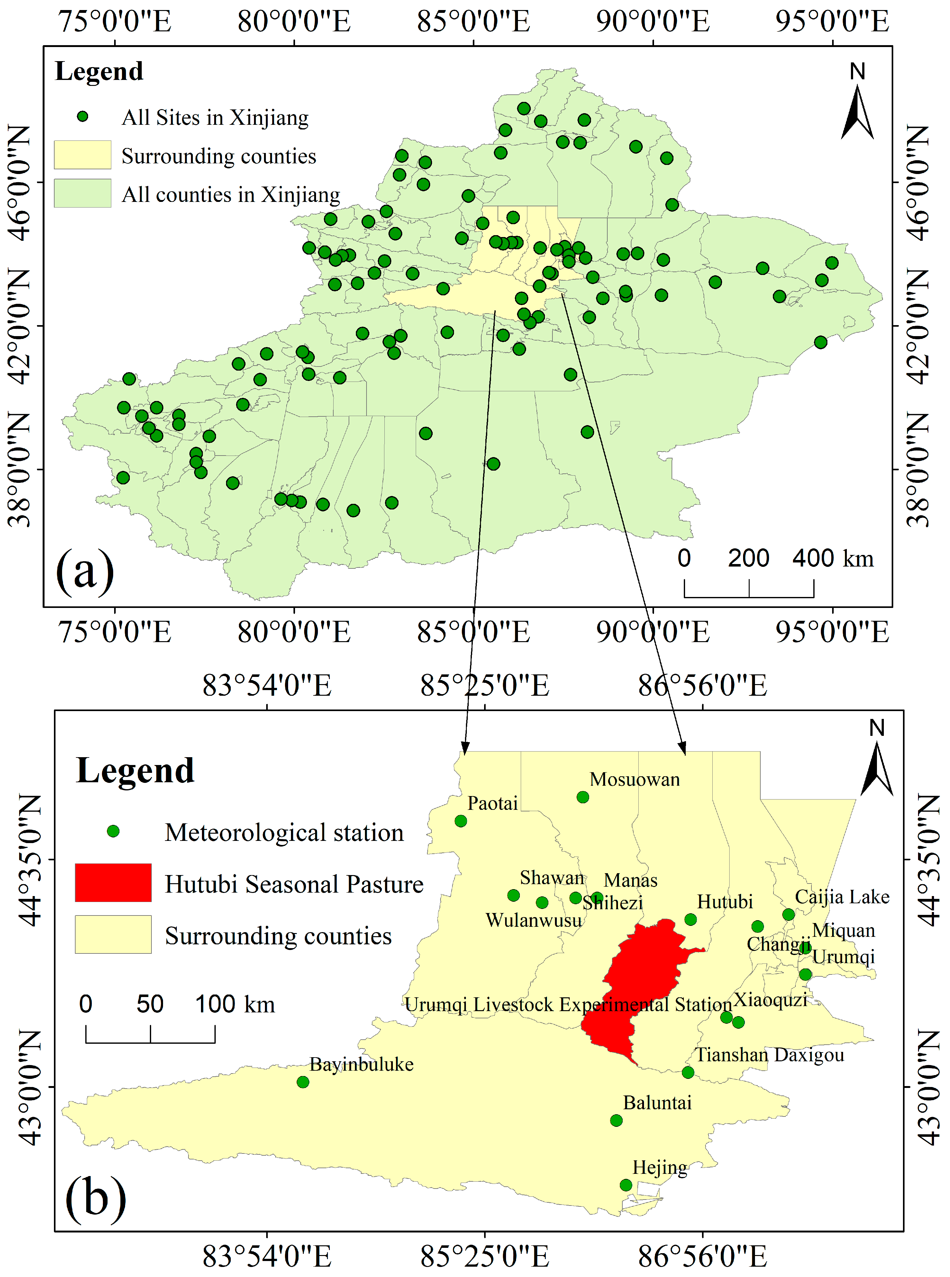
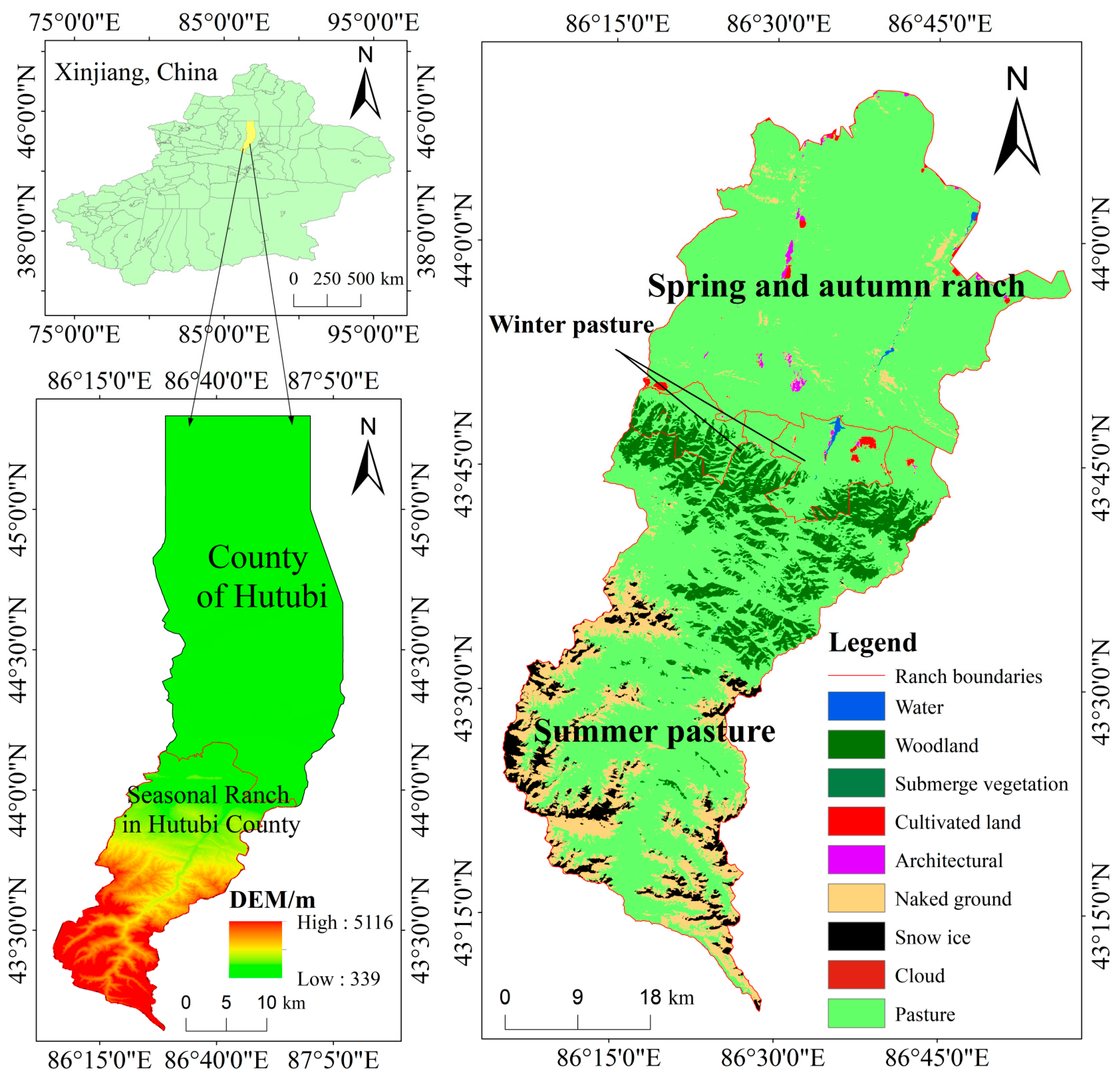
The study area was located in Hutubi County, Changji Hui Autonomous Prefecture, Xinjiang Uygur Autonomous Region, China, at the geographical coordinates 86°05′ E–87°08′ E and 43°07′ N–45°20′ N, and covered a total area of 9721.6 km². The study area exhibited a topography that was higher in the south and lower in the north, featuring high mountains and hills along the northern slope of the Tianshan Mountains in the south, alluvial plains in the central region, and desertified Gobi terrain in the north, forming a pronounced topographic gradient. This region was characterized by a typical temperate continental arid–semiarid climate, with an average annual temperature of approximately 6.7 °C, average annual precipitation of about 167 mm, and average annual sunshine duration of roughly 3090 h. These climatic conditions shaped a distinctive ecological landscape. Hutubi County had abundant vegetation resources, which mainly consisted of grasslands, meadows, alpine vegetation, and cultivated vegetation. Its pasture resources were particularly prominent, including multiple seasonal pastures such as the South Mountain pasture, Que’ergou Town pasture, and Yuanhu Village Town pasture. These pastures were categorized by grazing period into spring, summer, and winter pastures. The winter pasture was further subdivided into two spatially separate units, a left pasture and a right pasture. These pastures exhibited distinct seasonal variations in both time and space, providing an ideal setting for examining the dynamic effects of GP on NPP. An overview of the study area is shown in Figure 2.

2.2. Data Acquisition

2.2.1. Data Types and Sources

Estimating NPP using the CASA model required preparing multiple data types. These included NDVI data, vector data, meteorological data, and vegetation type data. Additionally, GP data and NPP product validation data were prepared. The specific data types and sources are detailed in

Table 1. Research Data and Sources.

Data Type	Description	Resolution	Source
NDVI data	Raster data: A July–August mean composite for the study area (mean compositing improves NDVI quality)	30 m	The Google Earth Engine (GEE) platform acquired Landsat 7/8 band data for computational processing.
Vector data	Vector data: Seasonal pasture polygons	/	College of Resources and Environment, Xinjiang Agricultural University.
Meteorological data	Raster data: Mean air temperature in August	30 m	Derived from the daily values dataset of basic meteorological elements from China’s national-level ground meteorological stations (Version 3.0).
	Raster data: Total precipitation in August	30 m	Derived from the daily values dataset of basic meteorological elements from China’s national-level ground meteorological stations (Version 3.0).
	Raster data: Total solar radiation in August	30 m	Derived from the daily values dataset of basic meteorological elements from China’s national-level ground meteorological stations (Version 3.0).
Vegetation type data	Raster data: China vegetation map at 1:1,000,000 scale	30 m	Source: National Geographic Conditions Monitoring Platform (http://www.dsac.cn).
Maximum Light Energy Utilization Rate	Tabular data: Parameter table for different vegetation types	/	Acquired from the literature data.
Grazing Intensity (GI)	Raster/Tabular data: GI dataset for grasslands in western China	250 m	https://figshare.com/articles/dataset/A_long-term_high-resolution_dataset_of_grasslands_grazing_intensity_in_China/26195684 URL (accessed on 10 July 2025)
Grazing Density (GD)	Tabular data: Annual ratio of total livestock numbers to pasture area (for GD derivation)	/	Xinjiang Uygur Autonomous Region Bureau of Statistics (https://tjj.xinjiang.gov.cn/).
Verification Data	Raster data: MODIS NPP product series	500 m	MODIS/Terra Net Primary Production Gap-Filled Yearly L4 Global 500 m SIN Grid V061 (LP DAAC catalog: lpcloud-mod17a3hgf-061).

.

2.2.2. Data Preprocessing

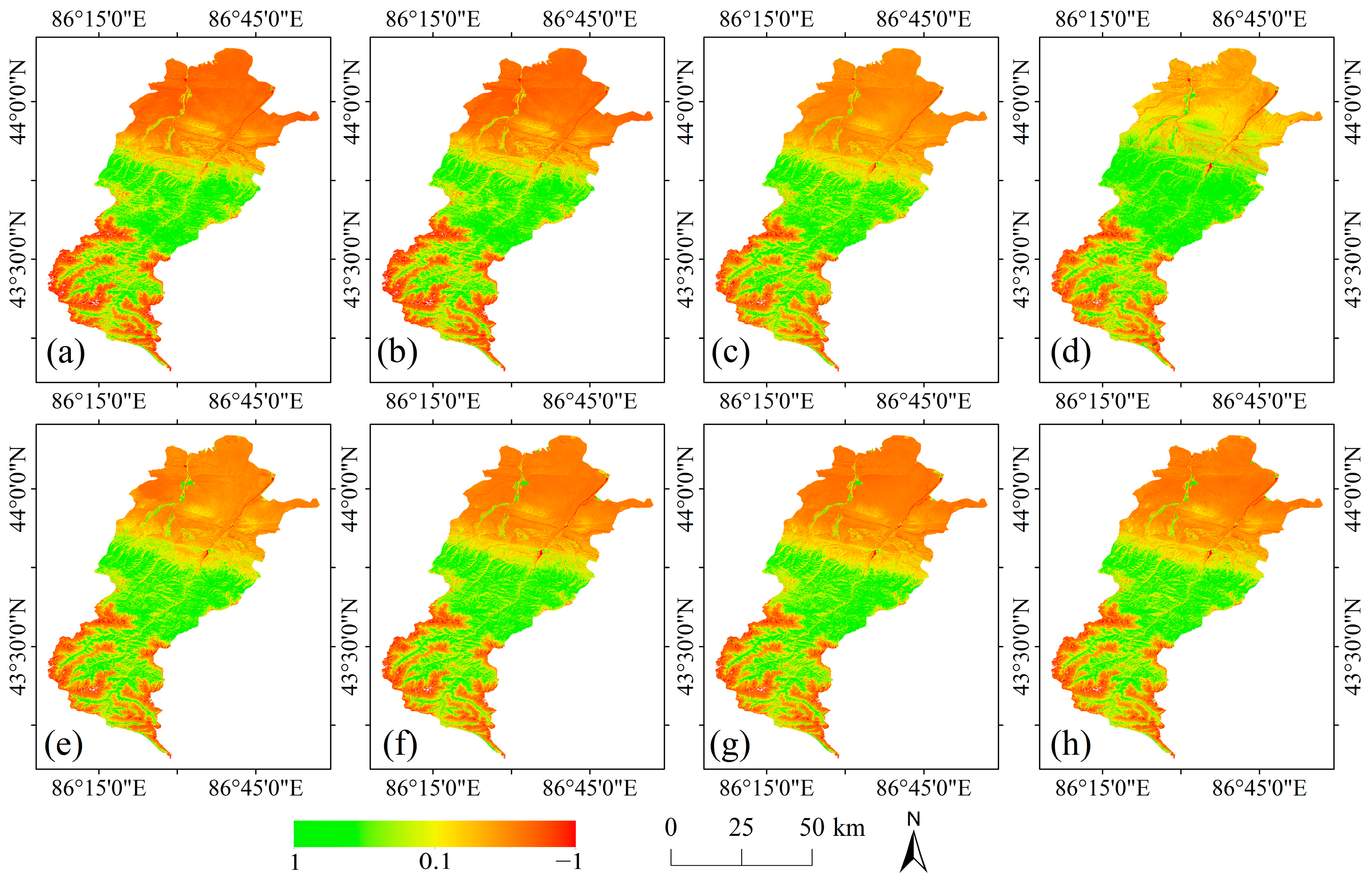
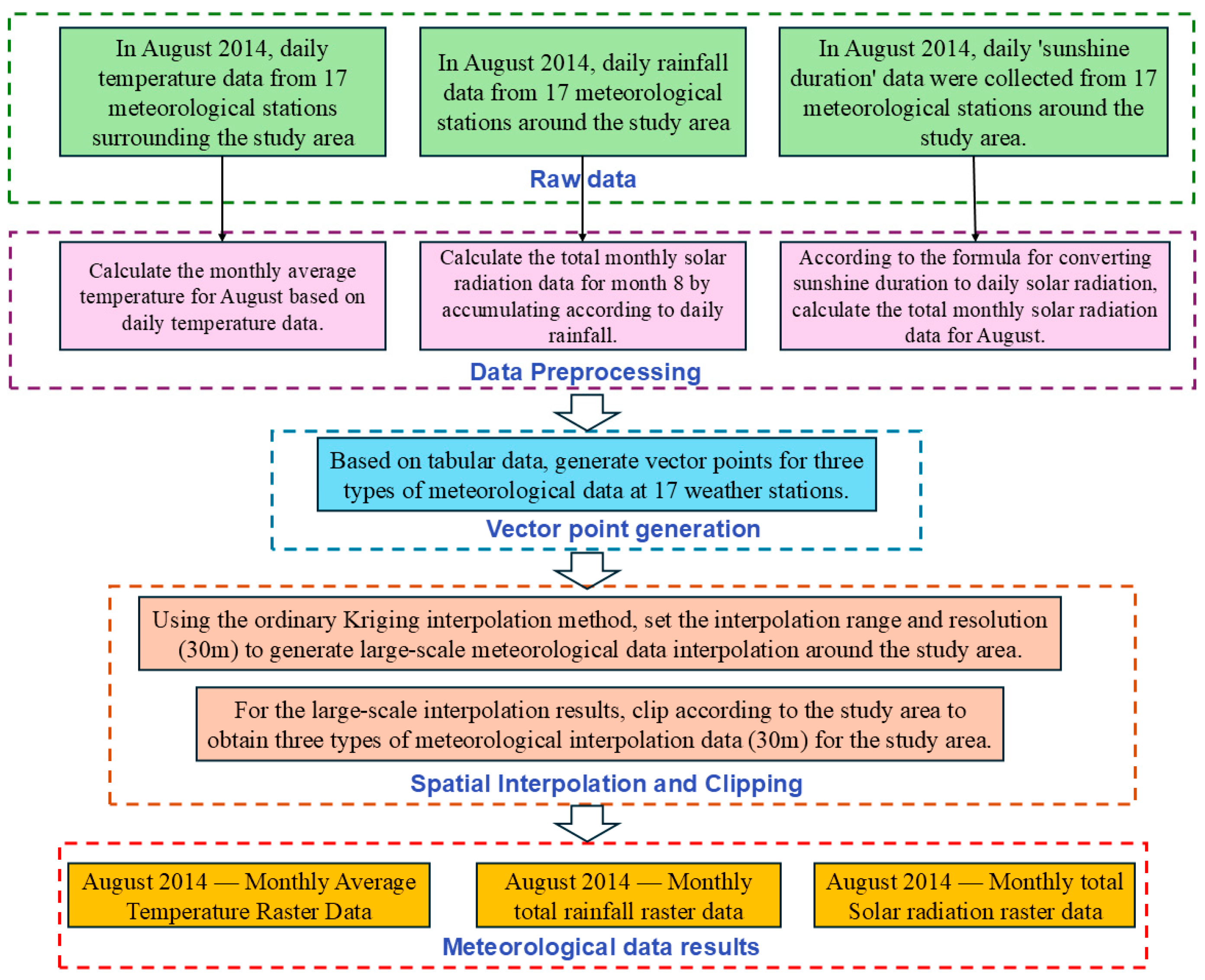
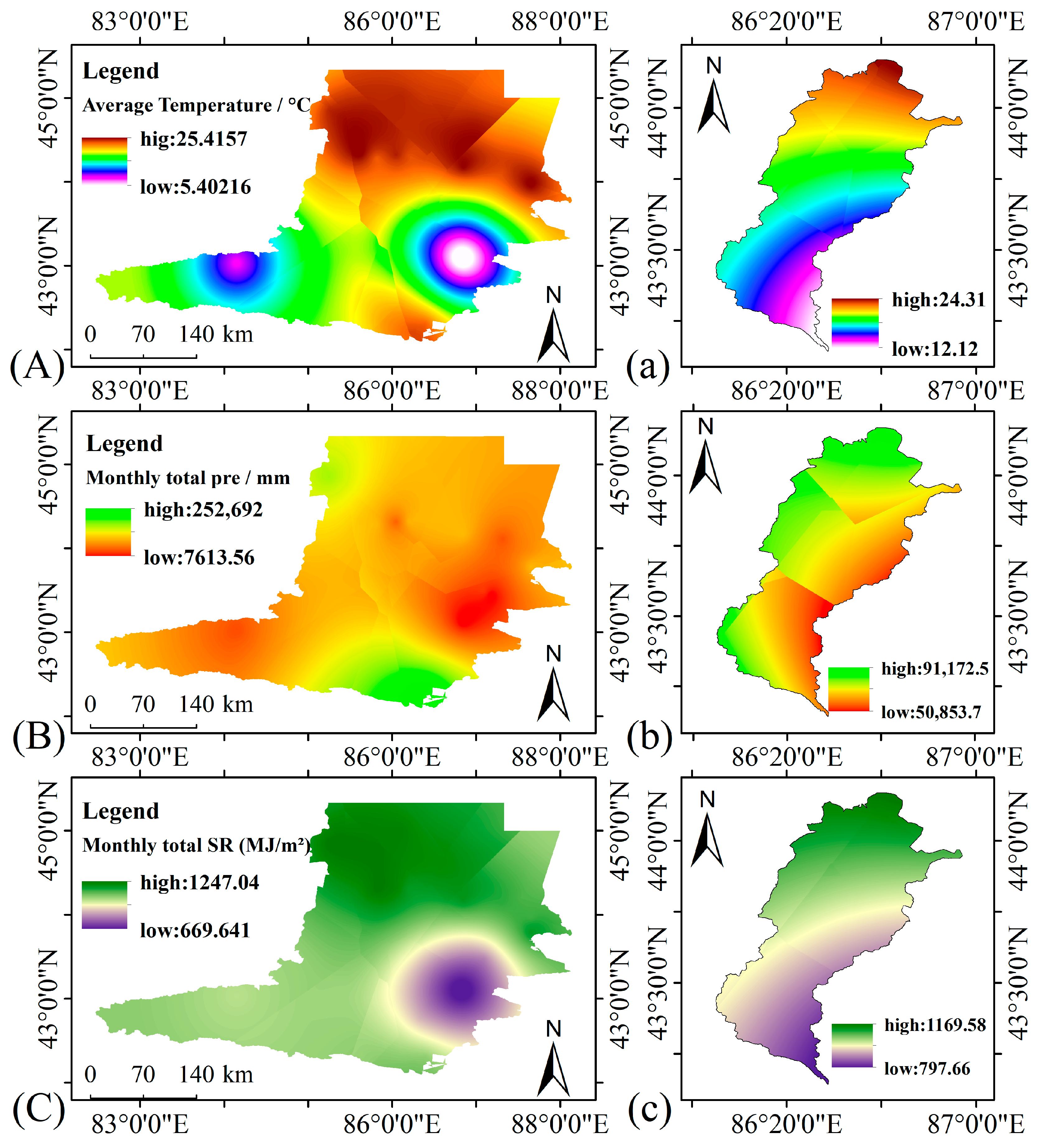
Before calculating NPP, we standardized all input datasets. (1) NDVI data: We computed NDVI for eight time periods between 2010 and 2024 using the GEE platform. When compositing NDVI, we used images from July–August to generate mean composites, because this approach could improve the quality of the NDVI estimates. (2) Vector data: These data were mainly used to clip the study area and included the overall seasonal pasture polygon as well as three internal seasonal pasture polygons (spring–autumn pasture, summer pasture, and winter pasture). (3) Meteorological data: We used daily August data for eight time periods between 2010 and 2024, obtained from the Daily Dataset of Basic Meteorological Elements at National Ground Meteorological Stations in China (V3.0). Point vector data for 17 meteorological stations surrounding the study area were generated and then converted to raster data using ordinary kriging interpolation, with a spatial resolution of 30 m (the detailed workflow was provided in Appendix D.1 and Appendix D.3). (4) Vegetation type data: We obtained a vegetation type map for the study area and converted the vector data to raster format to generate a vegetation type raster with a spatial resolution of 30 m (see Appendix D.4 for details). (5) Maximum light-use efficiency data: From the relevant literature, we obtained the maximum and minimum NDVI and SR values, as well as the maximum light-use efficiency (ε_max), for seven vegetation types in the study area. By matching these to the codes of each vegetation type, we produced a table of maximum light-use efficiency values to support the NPP calculations (see Appendix D.4,

Table A2. Total standardized sheep equivalent head count in Hutubi County (10,000 heads), 2010–2024.

Year	Cattle	Horses	Donkeys	Goats	Sheep	Total/(Sheep)
2010	39	6.48	0.15	2.824	39.28	87.734
2012	46.5	7.38	0.12	4.576	34.8	93.376
2014	47.55	7.56	0.09	6.056	31.45	92.706
2016	47.2	7.32	0.15	6.304	33.09	94.064
2018	39	2.7	0.09	1.008	24.07	66.868
2020	67.2	5.04	0.15	1.45	26.9	100.74
2022	55.95	2.16	0.12	1.23	30.63	90.09
2024	54	2.52	0.33	1.9	30.3	89.05

). (6) Grazing intensity data: We obtained raster datasets for eight time periods from 2010 to 2024 from an open dataset and clipped them to derive grazing-intensity maps for the study area. Based on these rasters, we calculated the annual mean GI for each of the eight time periods (the specific calculation formula was given in Section 3.2). (7) Grazing density data: Following the standard sheep unit conversion rules for livestock on the northern slope of the Tianshan Mountains [35] (Appendix A,

Table A1. Standard sheep equivalency rules for grazing livestock on the northern slope of the Tianshan Mountains.

Grazing Livestock	Cattle	Horses	Donkeys	Camels	Goats	Sheep
Standard sheep unit (head)	5	6	3	7	0.8	1

), different types of livestock were converted to a unified sheep unit, and the total converted livestock numbers were summarized (Appendix A, Table A2). The annually converted livestock totals were then divided by the area of each seasonal pasture to obtain GD data for each seasonal pasture in Hutubi County from 2010 to 2024 (Appendix A,

Table A3. Seasonal pasture GI in Hutubi County, 2010–2024.

Year	Pasture Name/GI (Sheep km−2 y−1)
	Spring–Autumn Pasture	Summer Pasture	Winter Pasture
2010	861.63	674.64	4803.13
2012	917.04	718.02	5112.01
2014	910.46	712.87	5075.33
2016	923.80	723.31	5149.68
2018	656.71	514.19	3660.79
2020	989.36	774.65	5515.16
2022	884.77	692.75	4932.11
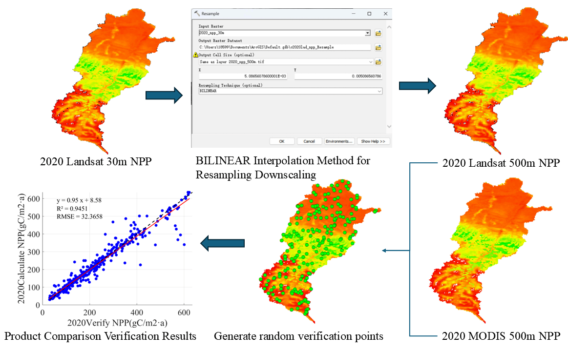
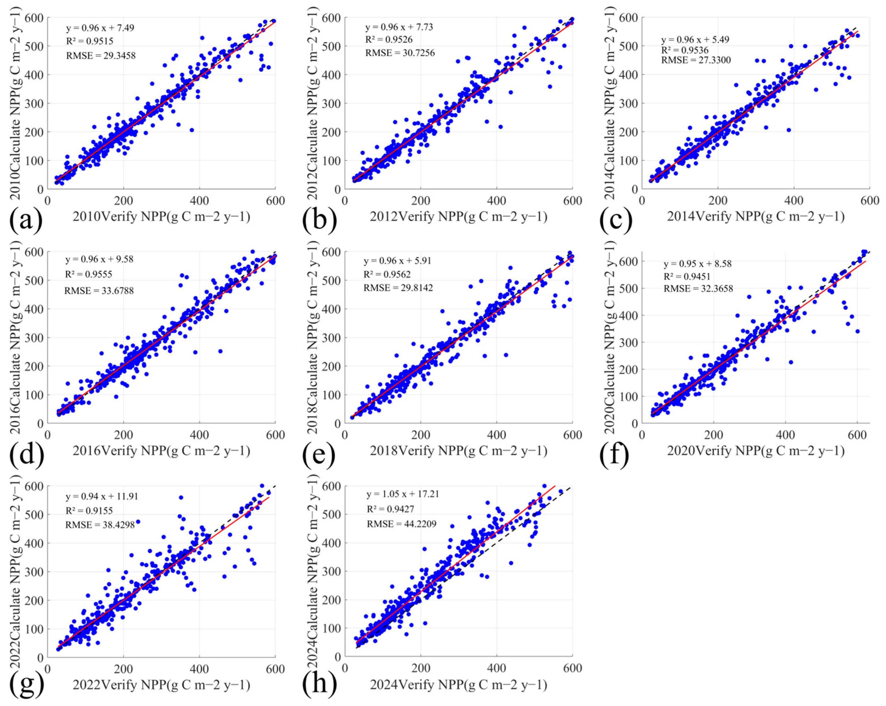
2024	874.56	684.76	4875.18

). (8) Validation data: We obtained MODIS NPP products with a spatial resolution of 500 m for eight time periods between 2010 and 2024 from an open dataset. These NPP products were clipped to the study area and used for product-based validation. The scale-matching between modeled NPP (30 m) and product NPP (500 m), as well as the validation procedure, was shown in Appendix D.5, Figure A8.

2.3. CASA Model

In this study, we used the CASA model, an ecosystem process model based on the principle of photosynthetic energy utilization. This model required inputs from remote-sensing data, air temperature, precipitation, solar radiation, and vegetation type data. We implemented the CASA model at a yearly time step in August (t), because that month corresponded to the peak vegetation growth season in the study area. Thus, the calculated NPP represented the monthly NPP for August, reflecting the maximum photosynthetic activity of each year rather than the annual total NPP. This time-step adjustment was appropriate for arid–semiarid grasslands, where vegetation growth and photosynthesis were strongly concentrated within a short growing season (typically July–August). Meteorological and radiation inputs (temperature, precipitation, and total solar radiation) were also extracted for August to maintain temporal consistency with the NDVI data. Using Equation (1), we estimated NPP from absorbed photosynthetically active radiation (APAR) and the photosynthetic energy conversion efficiency (ε), following the approach of Hadian et al. [36]:

$$NPP(x,t)=APAR(x,t)\times \epsilon (x,t)$$

(1)

where x represents any pixel in the image. NPP(x, t) denotes the NPP of pixel x at time t (g C m⁻² y⁻¹). APAR(x, t) denotes the APAR of pixel x at time t (MJ m⁻² y⁻¹). ε(x, t) denotes the ε of pixel x at time t (g C MJ⁻¹).

2.3.1. APAR Calculation

APAR served as the driving force for plant photosynthesis, showing a high correlation with plant biomass. It was also a key factor in the CASA model’s calculation of vegetation NPP, with its calculation given in Equation (2):

$$APAR(x,t)=SOL(x,t)\times FPAR(x,t)\times 0.5$$

(2)

where SOL(x, t) denotes the total solar radiation at pixel x and time t (MJ m⁻² month⁻¹). FPAR(x, t) denotes the fraction of photosynthetically active radiation absorbed by vegetation at pixel x and time t (dimensionless). The constant 0.5 indicates the ratio of effective solar radiation (0.38–0.71 μm) available for vegetation utilization. For SOL(x, t), when radiation data were unavailable, we derived it from sunshine duration. For FPAR(x, t), it can, in principle, be estimated from either the normalized difference vegetation index (NDVI) or the simple ratio vegetation index (SR) [37]. In practice, NDVI is typically used to derive FPAR in areas with moderate to high vegetation cover, whereas SR is more sensitive to reflectance changes under sparse vegetation and is therefore more suitable for estimating FPAR in low-cover environments. In this study, because the seasonal pastures in the study area generally had relatively high vegetation cover, we calculated FPAR(x, t) solely from NDVI, as given in Equations (3) and (4). For applications in sparsely vegetated areas, the SR-based FPAR formulation can still be found in Sun et al. [37]:

$$FPA{R}_{NDVI}={\displaystyle \frac{(NDVI-NDV{\mathrm{I}}_{min})\times (FPA{R}_{max}-FPA{R}_{min})}{(NDV{I}_{max}-NDV{\mathrm{I}}_{min})}}$$

(3)

$$NDVI(x,t)={\displaystyle \frac{NIR-R}{NIR+R}}$$

(4)

where NDVI_max, NDVI_min represent the maximum and minimum values of NDVI for different vegetation types, respectively. FPAR_max and FPAR_min denote the maximum and minimum values of FPAR for different vegetation types, respectively, and these two constants were set to 0.950 and 0.001, respectively [38]. NDVI(x, t) denotes the NDVI of pixel x at time t (dimensionless). NIR denotes the near-infrared band of the remote-sensing image, while R denotes the red band of the remote-sensing image.

2.3.2. ε Calculation

Actual light energy utilization efficiency (ε) refers to the ratio between the chemical energy contained in the dry matter produced by vegetation photosynthesis per unit area and time and the incident photosynthetically active radiation per unit area and time [39]. The formula for ε(x, t) is given in Equation (5):

$$\epsilon (x,t)=T_{\epsilon 1}(x,t)\times T_{\epsilon 2}(x,t)\times W_{\epsilon }(x,t)\times {\epsilon }_{max}$$

(5)

where T_ε1(x, t) and T_ε2(x, t) are dimensionless temperature-stress coefficients that describe the effects of low and high temperature, respectively, on vegetation photosynthetic efficiency. W_ε(x, t) is a dimensionless water-stress coefficient that reflects the effect of water availability on photosynthetic efficiency. ε_max denotes the maximum light-use efficiency for each vegetation type (g C MJ⁻¹). The values of ε_max for each vegetation type were obtained from the relevant literature.

The two temperature-stress coefficients, T_ε1(x, t) and T_ε2(x, t), are key variables for determining the actual light-use efficiency, and their calculation is given in Equations (6) and (7):

$$T_{\epsilon 1}(x,t)=0.8+0.002\times T_{opt}(x,t)-0.0005T_{opt}^2(x,t)$$

(6)

$$T_{\epsilon 2}(x,t)={\displaystyle \frac{\frac{1.1148}{\left\{1+exp\left[0.3\times \left(-T_{opt}(x,t)-10-T(x,t)\right)\right]\right\}}}{\left\{1+exp\left[0.2\times \left(T_{opt}(x,t)-10-T(x,t)\right)\right]\right\}}}$$

(7)

where T(x,t) denotes the average air temperature of the pixel during the time period. T_opt(x,t) denotes the optimal temperature for the growth of each vegetation type, which was estimated from the mean August temperature.

In this study, the water-stress coefficient ranged from 0.5 to 1.0, with values closer to 0.5 in drier areas and closer to 1.0 in wetter areas. Its calculation is given in Equation (8):

$$W_{\epsilon }(x,t)=0.5\times {\displaystyle \frac{E(x,t)}{E_p(x,t)}}+0.5$$

(8)

where E(x,t) represents the actual evapotranspiration (mm) and E_p(x,t) represents the potential evapotranspiration (mm).

2.3.3. Determination of Vegetation Static Parameters

The vegetation static-parameter file was used primarily to run the NPP computation module. It contains five components: vegetation code (Vege-code), the maximum and minimum of NDVI, the maximum and minimum of SR, and the maximum light-use efficiency (ε_max), which were obtained from the literature [40]. Using the 1:1,000,000 vegetation map, we identified seven vegetation types within the study area; the static parameters for each type are provided in Appendix D.4, Table A2.

2.4. GD Calculation

In this study, we employed GD to quantify GP, rather than the process-based “GI” defined within the NZSAP framework as the ratio of forage removal to available forage. GD represented the standardized number of livestock per unit area over a statistical period (year). It served as a stable proxy for GP at the regional scale, reflecting the spatial utilization intensity of grazing activities rather than the instantaneous proportion of forage removed.

To ensure comparability across different livestock types, the number of each livestock category was first converted into standard sheep equivalents using the standard sheep conversion factor commonly applied in the northern Tianshan region (see Appendix A Table A1). The total standardized livestock number SE_s,t for each pasture during season s in year t was then calculated using the following formula:

$$S{E}_{s,t}={\displaystyle \sum }_{j=1}^n{n}_{j,s,t}\times k_j$$

(9)

$$G{D}_{s,t}={\displaystyle \frac{S{E}_{s,t}}{A_{s,t}}}$$

(10)

where SE_s,t denotes the standardized total livestock count (head, converted to standard sheep equivalents) for seasonal pasture s in year t. n_j,s,t represents the number of livestock of category j (head) in seasonal pasture s during year t. k_j is the standard sheep equivalent conversion coefficient (dimensionless) for livestock category j. A_s,t represents the effective grazing area (km²) of seasonal pasture s in year t; GD_s,t denotes the GD (sheep km⁻²).

It should be noted that this study employed GD rather than process-based GI as a measure of GP. GI refers to the proportion of forage consumed relative to available forage within a unit time period, representing a process variable; GD denotes the standardized number of livestock per unit area, functioning as a spatial pressure variable. Due to the scarcity of high-resolution spatiotemporal data on forage production, consumption, and regeneration at the regional scale, it is difficult to obtain reliable estimates of GI. In contrast, GD is based on statistical livestock counts and grazing area, offering high data availability and strong repeatability, thereby enabling stable characterization of gradients in grazing utilization. Furthermore, GD and GI typically exhibit high interannual and spatial correlation, making GD a suitable observable proxy to reflect the negative feedback effect of GP on NPP. Therefore, this study employed GD as the key grazing indicator for threshold and NPP response analyses.

2.5. GI Calculation

In this study, we used the annual GI dataset developed by Wang et al. [25]. This dataset integrated climate-driven grassland productivity with satellite-remote-sensing biomass estimates, accounting for discrepancies between livestock numbers and available forage quantities. We employed this dataset for comparative analysis with the GD data collected in this study to assess which metric more accurately characterized GP. The core formula for calculating GI, used to estimate GI across counties and districts in the study area, is given below.

$$TS{U}_{p_j}={\displaystyle \sum }_{i=1}^{n}S{U}_{P_i}$$

(11)

$$S{U}_{Pi}={\displaystyle \frac{Agbliv{e}_{Pi}}{Agbliv{e}_s}}$$

(12)

$$Agbliv{e}_{Pi}=Agbliv{e}_{ci}\times (1+G_r)\times U_r\times S{H}_f$$

(13)

$$Agbliv{e}_s=S\times (1-W_r)\times C_f\times D$$

(14)

$$S{U}_{pasj}=\left\{\begin{array}{cc}S{U}_{cenj},& \mathrm{if} S{U}_{cenj}\le TS{U}_{pj}\\ TS{U}_{pj},& \mathrm{if} S{U}_{cenj}>TS{U}_{pj}\end{array}\right.$$

(15)

$$S{U}_{croj}=\left\{\begin{array}{cc}0,& \mathrm{if} S{U}_{cenj}\le TS{U}_{Pj}\\ S{U}_{cenj}-TS{U}_{Pj},& \mathrm{if} S{U}_{cenj}>TS{U}_{Pj}\end{array}\right.$$

(16)

$$S{U}_{pasi}=S{U}_{pasj}\times {\displaystyle \frac{Dif{f}_i}{{{\displaystyle \sum }}_{i=1}^{n}Dif{f}_i}}$$

(17)

where, in Equations (11)–(14), TSU_{P j} denotes the total potential livestock carrying capacity of county j; SU_{P i} represents the potential livestock carrying capacity of pixel i (unit: standard sheep units, SU); Agblive_{P i} indicates the available grassland biomass of that pixel (g C); Agblive_s represents the biomass consumed by one standard sheep per year; Agblive_{c i} denotes the baseline aboveground biomass of the pixel (g C); G_r represents the grassland regeneration rate; U_r indicates the grassland utilization rate; SH_f is the standard hay conversion factor; S is the daily hay ration per standard sheep (1.8 kg·SU⁻¹·day⁻¹); W_r denotes the standard hay moisture content (14%); C_f is the biomass-to-carbon conversion factor (0.45 g C·g⁻¹); D is the annual grazing days (365 days). In Equations (15)–(17), SU_{pas j} denotes the baseline livestock carrying capacity of grassland in county j; SU_{cen j} represents the livestock census data for county j; SU_{cro j} indicates the crop-based livestock carrying capacity for county j. SU_{pas i} denotes the grassland-based carrying capacity of county i; Diff_i represents the difference between climate-based and satellite-based biomass for pixel i; n is the number of grassland pixels in county j. The specific parameters and computational details are described in detail in Wang et al. [25].

2.6. Spatial Analysis (Graph Analysis Method)

Map analysis is a commonly used method for analyzing changes in land use types [41], with its calculation given by Equation (18).

$$M=10A+B$$

(18)

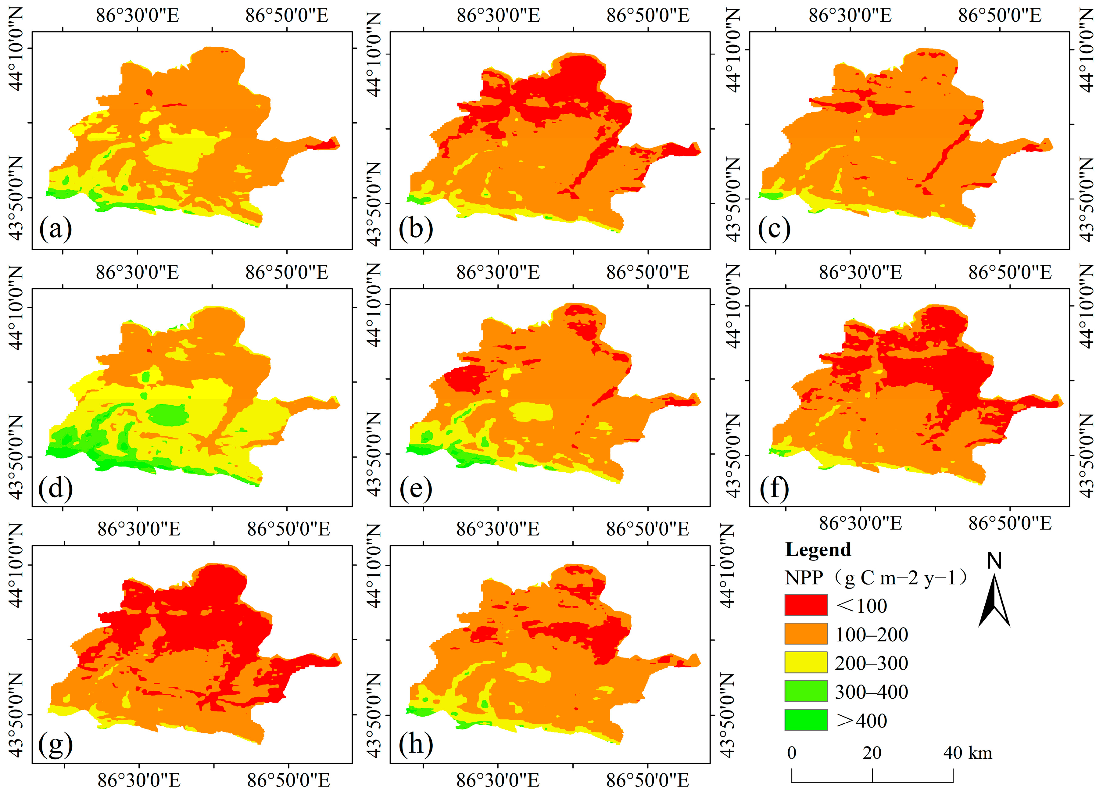
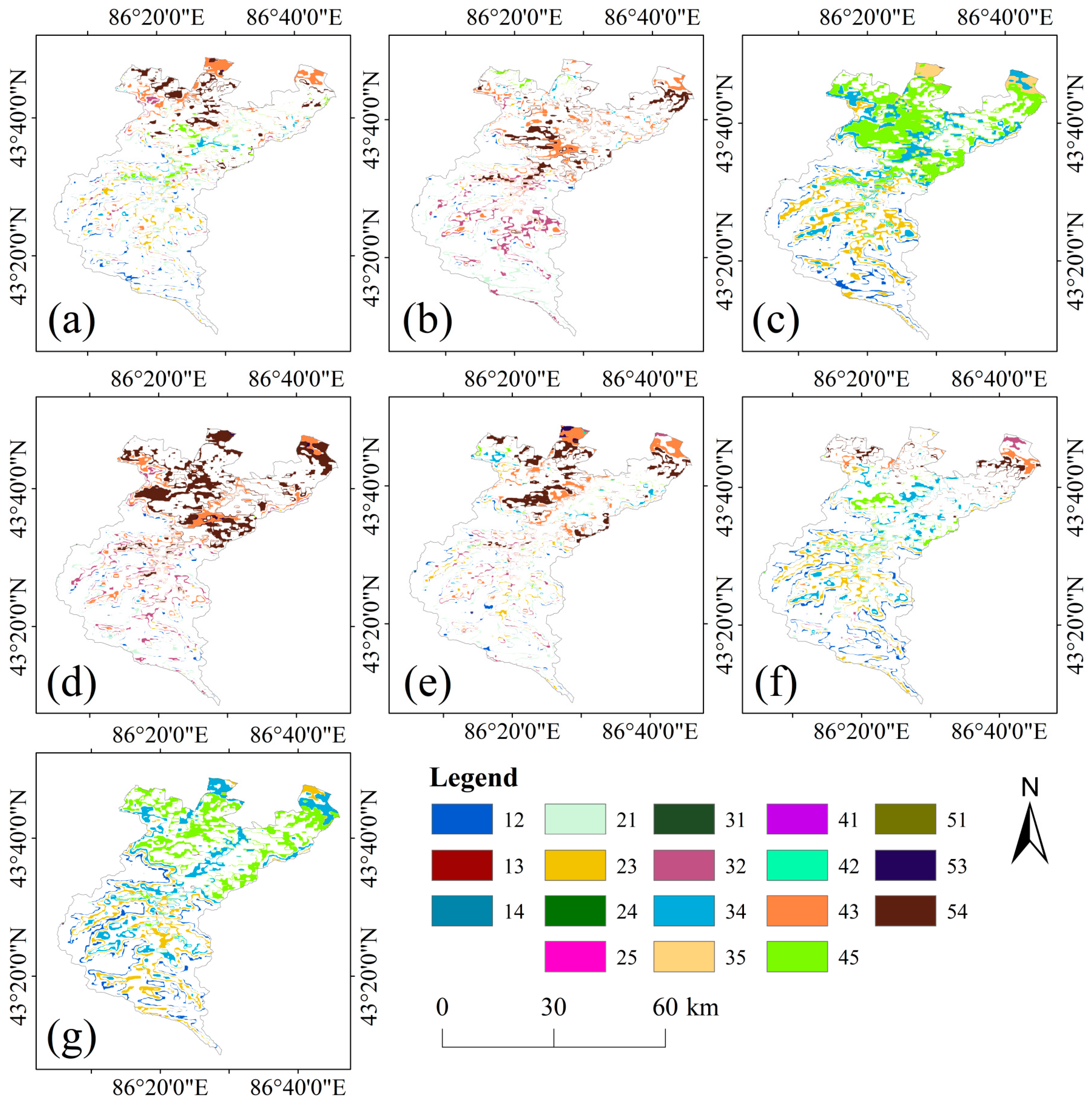
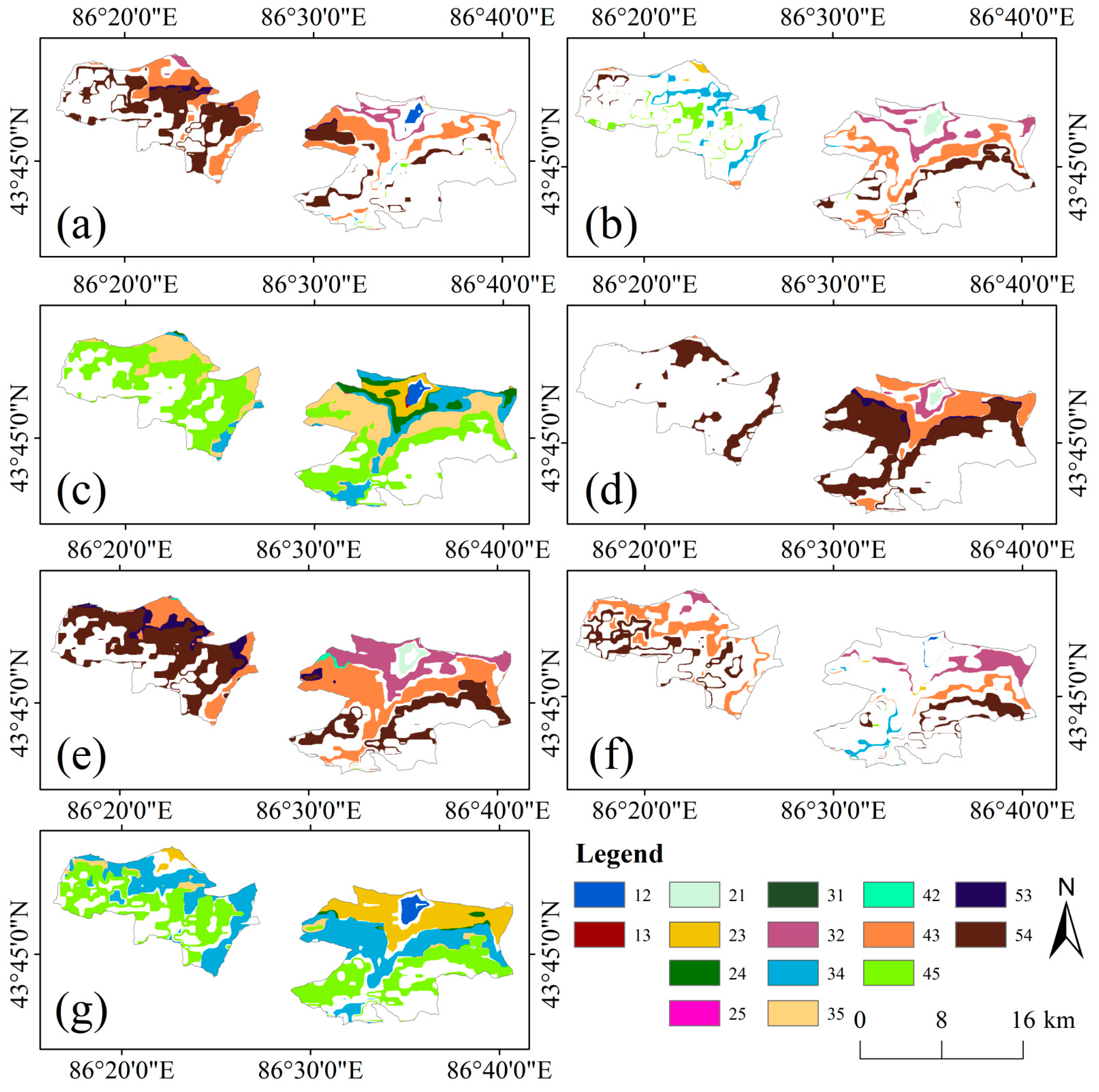
where M represents the NPP conversion code for a given period, A denotes the NPP class of the preceding year, and B denotes the NPP class of the subsequent year. Equation (8) was used to calculate the NPP class change for each pixel between the two periods (e.g., 21 indicates a conversion from class 2 NPP in 2010 to class 1 NPP in 2012). In this study, to facilitate the analysis of seasonal pasture NPP class changes, all annual NPP values were categorized into five classes based on NPP levels: below 100 g C m⁻² y⁻¹, 100–200 g C m⁻² y⁻¹, 200–300 g C m⁻² y⁻¹, 300–400 g C m⁻² y⁻¹, and >400 g C m⁻² y⁻¹. Higher classes indicated higher NPP values.

2.7. SEN-MK Trend Test

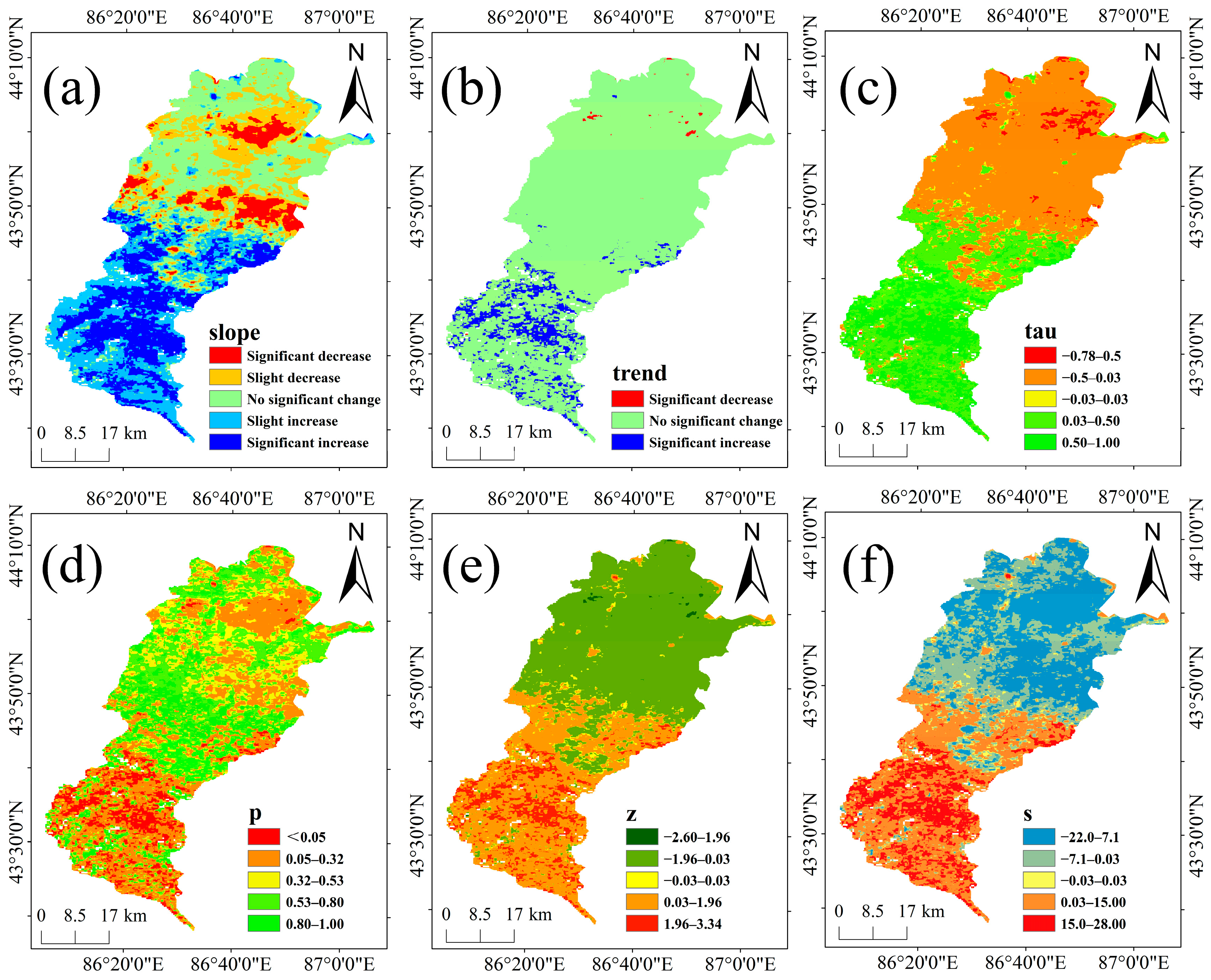
SEN-MK is a method for detecting trend changes in long-term time series data and performing significance tests on these changes. It comprises two components: Theil–Sen slope and Mann–Kendall trend. The Theil–Sen slope method, also known as Sen slope estimation, is a robust nonparametric statistical approach for trend calculation. This method offers high computational efficiency, is insensitive to measurement errors and outliers, and is suitable for trend analysis in long-term time series data [42]. In this study, the calculation formulas are given in Equations (19) and (20):

$$slop{e}_{i,j}={\displaystyle \frac{y_j-y_i}{j-i}} x_j\ne x_i$$

(19)

$$\beta =Median\left\{slop{e}_{i,j}\right\} \forall j>i$$

(20)

where slope_i,j denotes the slope value between paired observations i and j, representing the rate of change in observed values from time point i to time point j. y_j denotes the observed value at time point j; y_i denotes the observed value at time point i. i denotes an earlier index in the data sequence (ranging from 1 to n − 1), and j denotes the later index in the data sequence (ranging from i + 1 to n). In this formulation, β represents the estimated Theil–Sen slope, reflecting the overall rate of change trend across the entire time series, and Median { } denotes the median operator. If β > 0, this indicates an increasing trend in vegetation cover, whereas β < 0 indicates a decreasing trend in vegetation cover.

The Mann–Kendall trend test is a nonparametric method for assessing the significance of monotonic trends in time-series data. In this study, we summarized its outputs in five indicators. (1) Trend index: Based on the MK test results, we classified trends as increasing (1), decreasing (−1), or no trend (0). This index represented the MK test’s determination of trend direction; classification depended on the sign of Z and the p-value, without an explicit closed-form formula. Specifically, we used the following rules: if Z > 0 and p < α (e.g., 0.05), then “increasing” (1); if Z < 0 and p < α, then “decreasing” (−1); otherwise, “no trend” (0). (2) p-value: p was the significance indicator for the MK test, used to determine whether the trend was statistically significant (e.g., p < 0.05). (3) S-value: S was the Mann–Kendall score, reflecting the strength and direction of the trend. It was the fundamental statistic of the MK test; a positive S indicated an overall upward trend, a negative S indicated a downward trend, and a value close to 0 indicated no trend. (4) Tau value: τ (Kendall’s tau) was a standardized correlation coefficient associated with the MK test that quantified monotonic trend strength; τ > 0 indicated a positive (ascending) trend, τ < 0 indicated a negative trend, and values close to 0 indicated no monotonic trend. (5) Z-value: Z was the standardized test statistic serving as the significance measure for the MK test. It was calculated from S and its variance and was used to approximate the normal distribution. A positive Z indicated an upward trend, a negative Z indicated a downward trend, and |Z| > 1.96 (corresponding to p < 0.05 for a two-tailed test) indicated a statistically significant trend.

2.8. Performance Metrics (Accuracy Evaluation)

In this study, we evaluated model accuracy using a product-based validation approach, with RMSE and R² selected as the performance metrics. The corresponding formulas are given in Equations (21) and (22):

$$RMSE=\sqrt{{\displaystyle \frac{1}{n}}{\displaystyle \sum _{i=1}^n{(Y_i-y_i)}^2}}$$

(21)

$$R^2=1-{\displaystyle \frac{{\displaystyle {\sum }_{i=1}^n{(Y_i-y_i)}^2}}{{\displaystyle {\sum }_{i=1}^n{(y_i-Y_{mean})}^2}}}$$

(22)

where RMSE denotes the root mean square error, which shares the same units as the observed value Y_i and ranges from 0 to +∞. n represents the total sample size (the length of the time series or dataset). Y_i denotes the observed value for the i-th sample (e.g., the true NPP value), and y_i denotes the model-predicted value for the i-th sample. R² denotes the coefficient of determination, which is dimensionless and typically ranges from −∞ to 1. Y_mean denotes the arithmetic mean of all observed values Y_i.

3. Results

3.1. Validation and Trend Analysis of NPP in Seasonal Pastures of Hutubi County

3.1.1. NPP Validation of Seasonal Pastures in Hutubi County

An analysis of multi-year NPP calculations and product validation data for the study area revealed that the model exhibited high accuracy with minimal error (Figure 3). The R² values for NPP calculations across all eight periods exceeded 0.9, while the RMSE ranged between 27 and 45 g C m⁻² y⁻¹. Regarding correlation coefficients, R² exceeded 0.95 for the five periods from 2010 to 2018, while it fell below 0.95 for the three periods from 2020 to 2024. The maximum R² value occurred in 2018 (R² = 0.956), and the minimum was observed in 2022 (R² = 0.915). Regarding errors, the RMSE remained below 30 g C m⁻² y⁻¹ for the 2010, 2014, and 2018 periods (29.34, 27.33, and 29.81 g C m⁻² y⁻¹, respectively); meanwhile, the RMSE for the 2012, 2016, 2020, 2022, and 2024 periods remained above 30 g C m⁻² y⁻¹ (30.72, 33.67, 32.36, 38.42, and 44.22 g C m⁻² y⁻¹, respectively). Based on the 1:1 line, it was observed that, for the seven periods from 2010 to 2022, the calculated results showed good consistency with the product data when NPP was less than 450 g C m⁻² y⁻¹, but underestimation occurred when NPP exceeded 450 g C m⁻² y⁻¹. Additionally, the 2024 calculation results showed overestimation beyond 300 g C m⁻² y⁻¹. Based on the product comparison validation results, the CASA model demonstrated high accuracy and could be used to characterize seasonal variations in NPP in the study area’s pastures.

3.1.2. Analysis of Seasonal Pasture NPP Trends

Analysis and testing of multi-year NPP trends in the study area revealed significant changes in slope estimates for spring–autumn pastures and winter pastures, while slope estimates for summer pastures remained stable (Figure 4a). Trend changes were insignificant for spring–autumn pastures and winter pastures, but significant for summer pastures (Figure 4b). The significance levels were relatively low for spring–autumn pastures and winter pastures, while summer pastures exhibited better significance levels (Figure 4d). Specifically, slope estimation results indicated that spring–autumn pastures exhibited slight to significant decreasing trends in the central (86°50′0″ N) and southern (43°50′0″ N) regions, with most other areas showing no significant changes. Summer pastures exhibited slight to significant increases in lower-elevation mountainous areas (43°20′0″–43°50′0″ N). Winter pastures showed a significant increase in the southern region of the left pasture (primarily coniferous forest) and a significant decrease in the central region of the right pasture (mainly concentrated around lakes and farmland). Based on trend estimation results, spring/autumn and winter pastures showed no obvious trend changes in most areas except for a significant increase in some regions (44°0′0″ N), differing from slope results but confirming that NPP changes in spring/autumn and winter pastures were highly variable and exhibited nonlinear relationships over multiple years. Summer pastures in low-elevation mountainous areas exhibited a significant increasing trend, consistent with slope estimates, indicating that summer pasture NPP tended to increase over the years with a certain degree of linearity. Trend test results showed that Tau values for most areas of spring–autumn and winter pastures were less than −0.03, indicating slight to significant monotonically decreasing trends; p-values ranged from 0.05 to 0.32, indicating moderate significance levels. Z-values (−1.96 to 0.03) and S-values (−22.0 to 7.1) further underscored the substantial NPP fluctuations and relatively reliable trends in spring/autumn and winter pastures. Tau values for summer pastures were generally greater than −0.03; p-values below 0.05 indicated good significance; Z-values (1.96 to 3.34) and S-values (15.0 to 28) further demonstrated stable NPP variation in summer pastures, trending toward steady growth. The slope estimates and trend tests for multi-year NPP in the study area validated the overall NPP change patterns across seasonal pastures, providing a reference for subsequent analysis of interannual NPP variations in seasonal pastures.

3.2. Annual Variations in NPP of Seasonal Pastures in Hutubi County

3.2.1. Annual Variations in NPP of Spring and Autumn Pastures

Based on Figure 5, the overall trend of NPP variation at the spring–autumn pasture showed a decrease, followed by an increase, then another decrease before rebounding. The multi-year average NPP was 151.2 g C m⁻² y⁻¹, with a peak in 2016 (231.2 g C m⁻² y⁻¹) and a trough in 2022 (112.5 g C m⁻² y⁻¹). The most pronounced changes occurred in the northern part of the spring–autumn pasture (north of 44°0′0″ N), primarily within degradation levels 1–2. Additionally, significant changes were observed in the southern region (around 43°50′0″ N), mainly within degradation levels 3–5. In terms of NPP change levels by year, the patterns were as follows: In 2010 to 2012, degradation dominated, primarily at levels 21 and 32, concentrated in the northern areas near human activities. Between 2012 and 2014, NPP transitioned to recovery at level 12, with recovery areas distributed along the northern periphery. From 2014 to 2016, NPP recovery was dominated by grades 23 and 24, with significant improvement in the central and lower regions, particularly in the southernmost areas near winter pastures. From 2016 to 2018, degradation levels rose to 32 and 42, expanding the affected area to include the central region. From 2018 to 2020, degradation was primarily at levels 21 and 32, with degraded areas covering the central, northern, and eastern regions. From 2020 to 2022, degradation was primarily at level 21, with a few southern areas reaching level 3 NPP, while the central and northern regions decreased to levels 2 and 1, respectively. From 2022 to 2024, NPP recovery shifted to levels 12 and 23, with significant improvements concentrated in the central and western areas. Spatial distribution analysis indicated that NPP in the spring–autumn pasture exhibited gradient characteristics influenced by human activities. Northern areas near human activity zones exhibited lower NPP values and greater susceptibility to degradation. Central and western regions showed slower NPP fluctuations and higher recovery potential. Core NPP change zones were located in the north and center, reflecting the combined effects of GI and external disturbances. Based on these results, level 2 NPP changes occurred most frequently in the spring–autumn pastures, with common types including levels 12, 23, 21, and 32, indicating moderate fluctuation characteristics. NPP fluctuations in the spring–autumn pasture were pronounced and highly sensitive to GI and external factors (e.g., climate or policy interventions). The northern region exhibited particularly pronounced impacts from human activities, necessitating targeted management to enhance ecological stability.

3.2.2. Annual Variations in Summer Pasture NPP

As shown in Figure 6, the summer pasture was located at the southernmost part of the seasonal pasture system. Due to its distance from human activity areas, the overall variability in NPP at the summer pasture was relatively low. The multi-year average NPP was 255.1 g C m⁻² y⁻¹ with the lowest value recorded in 2014 (230.3 g C m⁻² y⁻¹) and the peak in 2016 (285.4 g C m⁻² y⁻¹). Regarding interannual NPP degradation levels, from 2010 to 2012, degradation dominated at levels 54 and 43, concentrated in the southern mountainous areas. From 2012 to 2014, degradation persisted, with levels 54 and 43 remaining predominant. From 2014 to 2016, NPP shifted toward recovery at grades 45, 34, and 23, with recovery areas expanding to the central and southern peripheries. From 2016 to 2018, degradation again dominated, with grades reverting to 54 and 43, primarily affecting the central region. From 2018 to 2020, degradation grades remained at 54 and 43, with the affected area further expanding. From 2020 to 2022, NPP shifted to recovery at levels 23 and 34, with the recovery zone covering the central and southern areas. From 2022 to 2024, recovery continued, with levels 45 and 34 predominating, significantly improving the ecology of central and southern pastures. Spatial distribution revealed a distinct gradient in summer pasture NPP. The southernmost snow-covered mountainous areas consistently exhibited NPP below 100 g C m⁻² y⁻¹, while central regions maintained NPP above 300 g C m⁻² y⁻¹ year-round, indicating stronger ecological stability. The core area of NPP variation lay in the southern mountainous transition zone, reflecting the combined effects of grazing and climate. Furthermore, NPP changes most frequently occurred at levels 3, 4, and 5, with common patterns including 4-5, 5-4, and 4-3. These patterns indicated that dynamic adjustments at medium-to-high levels constitute the primary ecological response characteristic of summer pastures. Summer pasture NPP exhibited lower sensitivity to GI compared to spring and autumn pastures, with changes primarily driven by environmental conditions and climatic factors in the southern mountainous areas. Optimizing stability would require integrating remote sensing monitoring with ecological management strategies.

3.2.3. Annual Variations in NPP at Winter Pastures

Based on Figure 7, the overall trend of NPP changes in the winter pasture showed a decrease, followed by a sustained increase, then a sustained decrease before rebounding. The multi-year average NPP was 391.8 g C m⁻² y⁻¹, with the lowest value occurring in 2022 (318.3 g C m⁻² y⁻¹) and the highest in 2016 (506.8 g C m⁻² y⁻¹). The primary areas of change were concentrated in two sections: the northern region of the left pasture (around 86°23′0″ N) and the northern region of the right pasture (around 43°45′0″ N). From the perspective of interannual NPP changes, from 2010 to 2012, NPP changes were dominated by degradation at levels 54 and 43, concentrated in the northern areas, particularly around water sources and cultivated land in the right pasture. From 2012 to 2014, degradation persisted at grades 43 and 54, primarily affecting the northern area of the right pasture. From 2014 to 2016, NPP transitioned to recovery at grades 45, 35, and 34, with the most pronounced recovery occurring in areas of the right pasture previously heavily impacted by human activities. From 2016 to 2022, NPP continued to degrade, primarily at levels 54, 43, and 32. Degradation expanded to the northern and eastern left-hand side areas, as well as the entire northern right-hand side. Vegetation degradation was particularly severe in human activity zones centered around lakes and farmland. From 2022 to 2024, NPP began to recover, primarily at levels 45 and 34, with the recovery area gradually expanding. Spatial distribution analysis revealed differentiated NPP patterns across winter pastures. NPP fluctuations remained relatively stable in the forest-dominated left side, constrained by natural conditions. In contrast, the natural grassland right side exhibited intense NPP volatility, with areas near lakes and farmland—significantly impacted by human activities—serving as core zones of change. Despite its small area, the winter pasture’s multi-year average NPP approached 400 g C m⁻² y⁻¹, indicating high vegetation productivity and restoration potential. Furthermore, NPP changes most frequently occurred between levels 4 and 5, with common transitions including 4⟶5, 4⟶3, 5⟶4, 3⟶4, and 3⟶5, reflecting dynamic adjustments between medium and high levels. The intense variability in winter pasture NPP was highly dependent on human activity intensity and climatic conditions in the right-side pasture area, while the left-side forested region exhibited greater stability. Enhancing ecological resilience required targeted management strategies.

3.3. Hutubi Seasonal Pasture GP Comparison

To determine which indicator—GI or GD—better characterized GP, we conducted a comparative analysis between an existing GI dataset and the GD dataset computed in this study. Based on Figure 8, interannual variations in GI differed markedly among seasonal pastures in Hutubi County: GI was generally stable in summer and winter pastures, whereas spring–autumn pastures persistently exceeded 2.0 sheep km⁻², indicating the strongest influence of grazing activities. Temporally, GI in spring–autumn pastures declined during 2010–2012, with weakening concentrated in the central, southern, and eastern sectors; rebounded in 2012–2014, with increases concentrated in the west and south; intensified further during 2014–2018, covering nearly the entire spring–autumn pasture except for small areas in the center; eased in 2018–2020, mainly across the west–central and southern areas; and decreased slightly in 2020–2022, with weakening concentrated in the north. During 2020–2024, GI increased slightly, with strengthened areas concentrated in the central–western and northern sectors; the northern sector showed the most pronounced increase. To further determine whether GI or GD better represented the actual level of GP in Hutubi County’s seasonal pastures, we conducted a comparative analysis of the relationships between GI/GD and annual mean NPP (Figure 9).

As shown in Figure 9, GI and annual mean NPP exhibited broadly synchronous interannual variations (i.e., they were largely in phase). This result suggested that GI could, to some extent, characterize regional GP. However, because GI was inferred from county-level livestock census data combined with satellite-derived grassland biomass differences (see Section 2.5), it was highly collinear with biomass itself, which might obscure the lagged effects of grazing on NPP and its significant negative correlation. By contrast, GD exhibited a stable negative relationship with NPP: increases in GD led to marked declines in NPP, whereas decreases in GD were associated with clear increases. A lag effect was also evident—after prolonged high-intensity grazing, NPP could continue to fall even if GD was reduced in the short term. For example, in Figure 9b, GD decreased during 2012–2014, yet NPP continued to decline. Based on the comparative analyses of GI and GD against the annual mean NPP, we ultimately adopted GD as the indicator for characterizing GP. For clarity, we thereafter used GD to denote GP in the analysis and proceeded to examine GD-driven changes in NPP across seasonal pastures.

3.4. Analysis of GD Effects on Seasonal Pasture NPP

The effect of GD on NPP in seasonal pastures was characterized by complex dynamic coupling. Multi-year GD–NPP comparisons for the three seasonal pastures (Figure 10) revealed a significant negative feedback between GD and NPP, together with a lagged NPP response to GD. Specifically, during 2010–2012, GD increased by 6.4%, and NPP declined across all three pasture types, with the largest decrease in the spring–autumn pastures (−31.14%), followed by winter (−9.16%) and then summer (−0.92%). During 2012–2014, GD fell by 0.7%; NPP rebounded in the spring–autumn pastures (+8.72%), whereas it declined in the summer (−6.73%) and winter (−4.72%) pastures. From 2014 to 2016, GD rose by 1.4%, yet NPP in all three pasture types increased markedly in an anomalous manner: spring–autumn (+70.32%), winter (+42.26%), and summer (+23.93%). From 2016 to 2018, GD decreased by 28.9%, but NPP continued to decline across all three pastures (also in an anomalous pattern): spring–autumn (−30.78%), winter (−17.11%), and summer (−11.14%). During 2018–2020, GD surged by 50.6%, and NPP continued to decline across all three pasture types: spring–autumn (−25.53%), winter (−17.34%), and summer (−3.89%). During 2020–2022, GD decreased by 10.6%; NPP still fell in the spring–autumn (−5.64%) and winter (−8.33%) pastures but rebounded in the summer pasture (+2.74%). During 2022–2024, GD fell by 1.2%, and NPP rose markedly across all three pastures: spring–autumn (+28.30%) > winter (+25.71%) > summer (+12.14%).

Taken together, the time-series evidence indicated a clear negative feedback between GD and NPP, with a nonlinear and lagged NPP response to GD. Spring–autumn pastures were most sensitive: even minor changes in GD could trigger pronounced shifts in NPP (e.g., 2022–2024); winter pastures were moderately sensitive; and summer pastures exhibit relatively stable NPP over the long term, suggesting weaker GD influence—likely related to their greater distance from settlements and higher elevations. The two anomalous phases were likely tied to policy and anthropogenic factors: the widespread NPP surge during 2014–2016 coincided with the implementation of the Grain-for-Green program and rest/closure grazing policies; by contrast, in 2016–2018, despite a sharp decline in GD, NPP continued to drop, largely due to elevated livestock inventories and extensive forage ensiling associated with pasture resting, which together suppressed NPP. Additionally, by analyzing the nonlinear fits of GD–NPP scatterplots and identifying significant change points in the Theil–Sen slopes, we determined grazing-density thresholds of 900 sheep km⁻² for spring–autumn pastures (Figure 10a), 700 sheep km⁻² for summer pastures (Figure 10b), and 5000 sheep km⁻² for winter pastures (Figure 10c). This procedure ensured the statistical robustness of the thresholds.

3.4.1. Impact of GD on NPP in Spring and Autumn Pastures

Under GD forcing, NPP class changes across the spring–autumn pasture were pronounced, with hotspots mainly north of 44°00′00″ N and south of 43°55′00″ N. The dominant change types were significant degradation (SD) and significant growth (SG): SD was chiefly 2⟶1 and 3⟶2, whereas SG was primarily 1⟶2 and 2⟶3. Specifically, during 2010–2012, GD increased by 6.4%, with SD accounting for 51.12% of the area (520.40 km²). The dominant SD types were 2⟶1 and 3⟶2, and the changes were concentrated in the southern sector adjacent to the winter pasture, the central zone (~86°35′00″ E), and the northern sector. During 2012–2014, GD decreased by 0.7%; SG rose to 22.72% (231.36 km²), while SD fell to 1.70% (17.26 km²). The dominant SG type was 1⟶2, concentrated in the northern sector. During 2014–2016, GD increased by 1.4%; SG was anomalously high at 67.74% (689.32 km²), dominated by 2⟶3 and 1⟶2 transitions, mainly in the central and southern sectors. During 2016–2018, GD decreased by 28.9%, yet the SD share rose to 61.2% (623.50 km²), dominated by 3⟶2, 4⟶3, and 3⟶1 transitions, mainly in the central and southern sectors. During 2018–2020, GD increased by 50.6%; SD accounted for 46.69% (475.52 km²), with 2⟶1 concentrated in the north and 3⟶2 concentrated in the central and southern sectors. During 2020–2022, GD decreased by 10.6%; SD accounted for 15.39% (156.67 km²) and SG for 2.67% (27.22 km²). SD was dominated by 2⟶1 and 3⟶2 transitions, scattered across the western and southern sectors, whereas SG (mainly 1⟶2) was concentrated in the eastern sector. During 2022–2024, GD decreased by 1.2%; SG rose to 43.69% (445.41 km²), dominated by 1⟶2 and 2⟶3 transitions, concentrated in the northern, southern, and eastern sectors.

Results indicated that the spring–autumn pasture experienced its sharpest shifts during 2014–2016 and 2016–2018: the former drove SG-dominated reorganization in the central and southern sectors, whereas the latter drove SD-dominated reorganization, with transitions occurring primarily between classes 3→2 and 2→3. Notably, during 2014–2016, NPP increased despite a slight rise in GD—likely reflecting policy-driven herd management that optimized GD and alleviated ecological stress. By contrast, in 2016–2018, degradation persisted even as GD dropped sharply, indicating a lagged response linked to an “ecological debt” accumulated under previously high GD (e.g., soil degradation and root damage), potentially further amplified by below-average spring–autumn rainfall. From the perspective of class-wise spatial responses, the northern sector of the spring–autumn pasture was dominated by 1→2 and 2→1 transitions (Figure 11a,b,e,g), indicating that class 2 NPP was most sensitive to disturbance under GD. The principal transition types were 1→2, 2→1, 2→3, and 3→2. Threshold analysis further showed that when GD exceeded the ecological carrying level of ~900 sheep km⁻², resource overuse triggered a soil–vegetation negative loop, leading to an expansion in the share of SD (Figure 11a,d,e). Conversely, a gradual reduction in GD tended to increase the share of SG, reinforcing the positive feedback of ecological recovery; however, if GP was rapidly eased over a short period, the benefit was often constrained by lag effects (Figure 11d). Policy factors were likewise non-negligible. For instance, the Grain-for-Green/Grassland Restoration program implemented during 2014–2016 substantially boosted NPP even when GD changed little (Figure 11c). Overall, as a seasonal transition zone, the spring–autumn pasture is highly sensitive to climatic fluctuations (e.g., shifts between wet and dry conditions). High-frequency, large-amplitude swings in GD tended to destabilize the ecosystem, whereas low-frequency, gradual adjustments were more conducive to building system resilience. Compared with single-season pastures, its threshold characteristics were more strongly shaped by policy and human activities, underscoring the need for integrated management strategies to maintain ecological balance.

3.4.2. Impact of GD on NPP in Summer Pastures

Under the influence of GD, most areas of the summer pasture maintained relatively stable NPP classes across periods, with changes concentrated in the central sector and the northern sector (north of 43°30′00″ N). SD transitions included 2→1, 3→2, 4→3, and 5→4, while SG transitions included 2→3, 3→4, 3→5, and 4→5. Specifically, during 2010–2012, GD increased by 6.4%; the SD area was 110.56 km² (8.49%), and the SG area was 15.36 km² (6.64%). SD was dominated by 5→4 and 4→3 transitions, concentrated in the northwestern sector, whereas SG was chiefly 2→3 and 4→5, mainly distributed in lower-elevation valleys in the south–central sector. During 2012–2014, GD decreased by 0.7%; the SD area rose to 118.56 km² (14.23%), with 5→4, 4→3, and 3→2 as the principal transitions, mainly in the central and northeastern sectors. During 2014–2016, GD increased by 1.4%; the SG area reached 486.77 km² (37.43%), dominated by 4→5, 3→4, and 2→3 transitions, concentrated in the central and northern sectors. During 2016–2018, GD decreased by 28.9%; the SD area was 268.26 km² (20.62%), dominated by 5→4, 4→3, and 3→2 transitions, concentrated in the central and northern sectors—largely coincident with the areas of NPP increase during 2014–2016. During 2018–2020, GD increased by 50.6%; the SD area was 162.29 km² (12.48%), dominated by 5→4 and 4→3 transitions, concentrated in the northwest and northeast. During 2020–2022, GD decreased by 10.6%; the SG area was 150.64 km² (11.22%), mainly 1→2, 2→3, and 3→4 transitions, concentrated in the central sector. During 2022–2024, GD decreased by 1.2%; the SG area rose to 386.84 km² (29.75%), dominated by 2→3, 3→4, and 4→5 transitions, primarily in the central and northern sectors. Results showed that, under the influence of GD, NPP class fluctuations in the summer pasture were relatively modest, with changes concentrated in the central and northern sectors and in lower-elevation valleys in the south. The reasons for the class shifts in 2014–2016 and 2016–2018 mirrored those in the spring–autumn pasture, but their magnitude was smaller because the summer pasture lay farther from settlements and was less affected by human activities. Threshold analysis indicated that when GD exceeded the ecological carrying level of ~700 sheep km⁻², the share of SD expanded (Figure 12b,d,e). Overall, the summer pasture’s class structure was dominated by medium–high classes, with changes most pronounced in classes 3 and 4, suggesting that under GD forcing, these two classes were the most disturbance-sensitive and prone to either degradation or growth. As a high-elevation seasonal pasture, it was sensitive to climatic fluctuations yet subject to relatively weak direct human disturbance; consequently, GD should be optimized within a coordinated framework of policy and climate-risk management.

3.4.3. Impact of GD on NPP in Winter Pastures

Under GD forcing, the winter pasture exhibited pronounced NPP class dynamics, with changes concentrated in the northern sector of the left pasture and the central–western and northern sectors of the right pasture. The dominant SD transitions were 5→4, 4→3, and 3→2, while the dominant SG transitions were 4→5, 3→5, and 3→4. Overall, NPP classes remained at medium–high levels, chiefly in classes 4 and 5. Specifically, during 2010–2012, GD increased by 6.4%; SD accounted for 36.9% (67.39 km²), with 5→4 and 4→3 transitions concentrated in the northern sector of the left pasture and the western sector of the right pasture. During 2012–2014, GD decreased by 0.7%; SD accounted for 17.18% (31.39 km²), again dominated by 5→4 and 4→3 transitions, mainly in the central and northern sectors of the right pasture. SG accounted for 6.2% (11.37 km²), chiefly 3→4 and 4→5 transitions, concentrated in the northern sector of the left pasture. During 2014–2016, GD increased by 1.4%; SG accounted for 70.1% (128.17 km²), dominated by 3→4, 3→5, and 4→5 transitions, distributed across the northern and eastern sectors of the left pasture and the western, central, and northern sectors of the right pasture. During 2016–2018, GD decreased by 28.9%; SD accounted for 38.49% (72.29 km²), dominated by 5→4 and 4→3 transitions, concentrated in the central, western, and northern sectors of the right pasture. During 2018–2020, GD increased by 50.6%; SD accounted for 63.10% (115.23 km²), with degradation still dominated by 5→4, 4→3, and 3→2 transitions. The northern sector of the left pasture was chiefly 5→4, whereas the central, western, and northern sectors of the right pasture were dominated by 4→3 and 3→2. During 2020–2022, GD decreased by 10.6%; SD accounted for 24.18% (44.19 km²), again dominated by 5→4, 4→3, and 3→2 transitions, distributed in the western sector of the left pasture and the eastern sector of the right pasture. During 2022–2024, GD decreased by 1.2%; SG accounted for 74.08% (135.30 km²), dominated by 3→4, 3→5, and 4→5 transitions. Changes were concentrated in the northern sector of the left pasture and in the central, western, and northern sectors of the right pasture. In particular, the northern sector of the right pasture was dominated by 3→5 transitions, indicating strong ecological recovery.

Results indicated that, like the spring–autumn pasture, the winter pasture exhibited pronounced NPP class fluctuations under GD; however, its dominant transition classes were closer to those of the summer pasture, with most areas clustering in classes 4–5. Due to the subdivision into left and right sectors and underlying vegetation differences, the winter pasture exhibited spatial heterogeneity in its class-change range. In the left sector, the south was forested and showed modest NPP variability, whereas the northern area adjacent to the spring–autumn pasture was more strongly affected by GD. In the right sector, pronounced NPP fluctuations occurred around lakes and croplands, reflecting substantial human disturbance; the main change zones lay in the central and western parts, with transitions predominantly involving classes 3 and 4. Additionally, threshold analysis indicated that when GD exceeded ~5000 sheep km⁻², the share of SD expanded (Figure 13a,d,e). Overall, compared with the summer and spring–autumn pastures, the winter pasture exhibited generally higher NPP classes and a stronger response to GD. Therefore, optimizing winter-pasture management required scientific grazing zoning and stricter regulation of human activities.

4. Discussion

4.1. GD and NPP Exhibit a Negative Correlation

At the seasonal-pasture scale, GD and NPP exhibited an overall negative relationship that was strongly modulated by thresholds: when GD exceeded the threshold, the grassland system entered a degradation phase, whereas remaining below the threshold facilitated recovery. Specifically, the Sen–MK results (p < 0.05) revealed a long-term negative association between GD and NPP across all three seasonal pastures, and the seasonal-pasture comparisons of GD with annual mean NPP (Figure 10) further substantiated this interannual negative correlation. Similarly, Ahmed et al. [43] showed that high GP significantly reduced ANPP. However, because precipitation is strongly positively correlated with ANPP, forage exhibits greater grazing tolerance in wet seasons; consequently, the negative GD–NPP association is less significant in wet seasons than in dry seasons. Additionally, Gao and Gong [6,44] emphasized a strong negative relationship between GP and BNPP. They reported that heavy grazing significantly reduces live root biomass and BNPP; moreover, BNPP contributes roughly 60% of NPP dry-matter accumulation, implying that increases in GP substantially depress BNPP and thereby strongly affect NPP dynamics.

The negative GD–NPP relationship was regulated by GD thresholds, which were approximately 900, 700, and 5000 sheep km⁻² for the spring–autumn, summer, and winter pastures, respectively (Figure 10a–c). When GD exceeded the threshold, the share of SD increased by ~30%; conversely, under sub-threshold, appropriately managed grazing, the share of SG increased by ~25% (Appendix B,

Table A5. Effects of GI on changes in summer pasture NPP levels.

Year	GI/(Sheep km−2 y−1)	Rate of Change in GI/%	NPP Grade Change			Area Ratio/(%)
			NC	SD	SG	NC	SD	SG
2010–2012	674.64→718.02	6.4	11, 22, 44, 55	54, 43, 21, 32	23, 45, 12, 34	84.87	8.49	6.64
2012–2014	718.02→712.87	−0.7	11, 22, 44, 33	54, 43, 21, 32	/	84.86	14.23	/
2014–2016	712.87→723.31	1.4	11, 22, 55, 33	/	45, 34, 23, 35	62.16	/	37.43
2016–2018	723.31→514.19	−28.9	11, 55, 22, 33	54, 43, 32, 21	/	78.56	20.62	/
2018–2020	514.19→774.65	50.6	11, 22, 33, 44	54, 43, 32, 21	/	84.86	12.48	/
2020–2022	774.65→692.75	−10.6	11, 44, 33, 22	/	23, 34, 12, 45	84.87	/	11.22
2022–2024	692.75→684.76	−1.2	11, 55, 33, 44	/	45, 34, 23, 12	70.04	/	29.75

,

Table A6. Effects of GI on changes in winter pasture NPP levels.

Year	GI/(Sheep km−2 y−1)	Rate of Change in GI/%	NPP Grade Change			Area Ratio/(%)
			NC	SD	SG	NC	SD	SG
2010–2012	4803.13→5112.01	6.4	55, 44, 33, 22	54, 43, 32, 53	/	61.68	36.9	/
2012–2014	5112.01→5075.33	−0.7	55, 44, 33, 22	43, 54, 32	34, 45	76.62	17.18	6.2
2014–2016	5075.33→5149.68	1.4	55, 22, 44, 33	/	45, 35, 34, 24	29.9	/	70.1
2016–2018	5149.68→3660.79	−28.9	55, 44, 33, 22	54, 43, 32, 53	/	61.51	38.49	/
2018–2020	3660.79→5515.16	50.6	55, 44, 33, 22	54, 43, 32, 53	/	36.88	63.10	/
2020–2022	5515.16→4932.11	−10.6	44, 33, 55, 22	54, 43, 32, 21	/	74.55	24.18	/
2022–2024	4932.11→4875.18	−1.2	55, 44, 33, 22	/	45, 34, 23, 35	25.92	/	74.08

and

Table A7. Changes in NPP classes and their areas at Hutubiqi spring pasture from 2010 to 2024.

2010–2012		2012–2014		2014–2016		2016–2018		2018–2020		2020–2022		2022–2024
Level	Area/km2	Level	Area/km2	Level	Area/km2	Level	Area/km2	Level	Area/km2	Level	Area/km2	Level	Area/km2
11	9.702	11	63.10	11	0.446	11	0.371	11	56.31	11	327.7	11	127.4
12	0.036	12	224.8	12	67.19	12	0.074	12	31.16	12	26.60	12	331.3
21	275.7	21	4.661	13	0.128	21	67.77	21	298.0	21	131.1	21	3.705
22	443.3	22	647.5	22	325.1	22	324.6	22	437.3	22	475.3	22	422.7
23	0.210	23	5.377	23	466.5	23	0.001	23	0.728	23	0.626	23	96.97
31	2.499	32	11.27	24	91.08	31	19.33	32	132.7	32	21.51	24	0.090
32	213.6	33	54.05	25	0.851	32	405.7	33	17.06	33	31.14	32	0.112
33	39.41	34	1.123	33	2.990	33	44.55	34	0.014	43	4.033	33	18.82
34	0.019	43	1.304	34	30.26	42	5.660	42	5.862	44	0.205	34	15.93
42	0.576	44	5.016	35	27.47	43	102.1	43	28.02			35	0.939
43	26.79	54	0.029	44	0.009	44	13.50	44	0.118			44	0.112
44	5.105			45	6.160	45	0.054	53	6.832			45	0.092
45	0.005					53	3.102	54	4.105
53	0.036					54	20.50
54	1.195					55	10.88
55	0.024

Note: Blue boxes indicate no change in NPP level (NC) for the corresponding year; green boxes indicate an increase in NPP level (SG) for the corresponding year; and yellow boxes indicate a decrease in NPP level (SD) for the corresponding year. Bold red text denotes the predominant type among different level changes.

). This indicated that grassland ecosystems in different seasonal pastures triggered the GD–NPP negative feedback at distinct grazing-density thresholds. Similarly, Guifeng [45] reported that when GD exceeded 8.17 sheep hm⁻² in spring–autumn pastures, 5.19 sheep/hm² in summer pastures, and 12.41 sheep hm⁻² in winter pastures, soil erosion increased by about 15.57–20.65%, and NPP declined by roughly 23%. Therefore, once the GD in a seasonal pasture exceeded its threshold, a negative feedback was triggered. Nevertheless, the GD thresholds reported here were identified from a limited set of eight time periods using a morphology-based procedure; their statistical robustness and confidence intervals require further verification. Moreover, GD was highly sensitive to local policy interventions—for example, the 2014–2016 Grain-for-Green/Grassland Restoration program substantially altered GD dynamics [46]. In addition, NPP is strongly modulated by precipitation: the negative GD–NPP feedback is less pronounced in wet seasons than in dry seasons [43]. Despite these limitations, our results provided important evidence for understanding threshold characteristics of grassland ecosystems in arid and semi-arid regions and the mechanisms linking GD to NPP. They further suggested that management should prioritize areas approaching or exceeding the thresholds, implementing measures such as stocking limits, off-season grazing, and rotational grazing to reduce degradation risk and enhance system recovery capacity.

4.2. The Impact of GD on Seasonal Pasture NPP Varies

The NPP response to GD varied across seasonal pastures, reflecting heterogeneity tied to geographic setting, vegetation type, and land use; pertinent geographic factors included pasture location, topography/elevation, and climate. Specifically, the spring–autumn and winter pastures lay closer to zones of human activity and thus exhibited higher NPP sensitivity to GD. For example, during 2010–2012, when GD increased by 6.4%, the SD share reached 51.12% in the spring–autumn pasture and 36.9% in the winter pasture, whereas in the summer pasture—farther from human activity—the SD share was only 8.49%. Similarly, Li et al. [47] noted that human activities were the primary driver of NPP degradation, with more intensive activity associated with more pronounced declines. This implied that seasonal pastures located closer to human activity zones were more ecologically fragile, and their NPP was more prone to sharp changes under GD. In addition, in the southern sector of the summer pasture, high-elevation mountainous areas exhibited higher and more stable NPP (multi-year mean ≈ 255.1 g C m⁻² y⁻¹), whereas areas near perennial snow/ice farther south consistently remained below 100 g C m⁻² y⁻¹. Cao et al. [48] reached a similar conclusion, noting that global NPP was strongly regulated by climate and topography, with climatic controls outweighing those of elevation. This underscored both the constraining effect of rugged terrain on grazing activities and the influence of high-elevation climates on enhancing vegetation NPP. Beyond geographic setting, vegetation type and land use also shaped NPP sensitivity to GD. For example, in the southern part of the left-hand winter pasture, where coniferous forest predominated, NPP had remained stable over many years and was less affected by GD. By contrast, the right winter pasture was largely natural grassland, where NPP classes fluctuated markedly over time and responded more sensitively to GD. Additionally, in the right winter pasture, lake and cropland areas experienced frequent human disturbance, and multi-year NPP class changes were dominated by SD. This was consistent with Gao Z. et al. [49], who noted that different land use types can either increase or decrease NPP and thus affect vegetation carbon storage, but these effects were insufficient to offset the negative impacts of climate change. These findings indicated that vegetation type and land use substantially shaped the sensitivity of NPP to GD, although climatic influences could not be overlooked. Given the heterogeneous GD–NPP responses across seasonal pastures, differentiated management was recommended. For example, rest-grazing zones should be established in the northern portion of the spring–autumn pasture to mitigate pronounced human impacts; ecological protection should be strengthened in the southern summer pasture to preserve the stability of high-elevation mountain ecosystems; in the right winter pasture, rotational grazing and targeted subsidies should be implemented to curb the adverse effects of land use. Meanwhile, local forestry and grassland agencies could combine climate models (e.g., RegCM4.4 simulations driven by CMIP) to assess the potential impacts of extreme climate events on pastoral NPP [50,51]. By introducing real-time GD monitoring and early-warning mechanisms, an ecological–livestock balance could be achieved, providing practical support for the long-term sustainable management of grasslands on the northern slope of the Tianshan Mountains.

4.3. Uncertainty Analysis and Outlook

Despite elucidating the negative GD–NPP relationship and its threshold behavior, several uncertainties remained. (1) Potential inflation of GD magnitudes due to the measurement scheme: Because GD was defined as “standard sheep units per pasture area”, it captured the negative GD–NPP relationship better than other GI products, but it could numerically inflate GD in small-area pastures (e.g., the winter pasture). Importantly, this did not alter the relative pattern of GP (winter > spring–autumn > summer) [45]. (2) Limitations of the CASA model: CASA was relatively insensitive to soil-moisture stress, which could lead to NPP overestimation—especially in high-GD areas—so recovery potential might have been overstated. High-resolution soil datasets were needed for calibration [52]. (3) Precipitation and temperature not incorporated: This study focused on GD as a single driver and did not jointly analyze climatic factors such as precipitation and temperature, limiting the interpretation of anomalous years and potentially underrepresenting the complexity of the GD–NPP relationship [5,53]. Building on these uncertainties, future work could use UAVs and GPS to finely monitor grazing trajectories and refine GD estimation [54,55]; in parallel, intensifying field plot surveys and flux observations would enable better CASA parameterization and independent validation of trend results. Moreover, incorporating climatic variables within a multifactor regression framework will be needed to examine threshold dynamics under GD–climate interactions [56]. These enhancements would improve the precision and robustness of the analysis and provide a stronger evidence base for the sustainable management of grasslands on the northern slope of the Tianshan Mountains.

5. Conclusions

Our study showed that the GD–NPP relationship was a nonlinear negative correlation modulated by threshold effects. In addition, the proposed GD estimation method was simpler and more practical than alternative measures of GP, and it captured the negative feedback between GP and NPP; as such, it provided a viable proxy for actual GP. When GD exceeded the threshold, NPP began to degrade; when GD remained below the threshold, NPP tended to recover. Marked heterogeneity existed across seasonal pastures: the spring–autumn and winter pastures—shaped by geographic setting and vegetation type—were most sensitive to GD and exhibited the largest fluctuations in NPP classes, whereas the summer pasture, constrained by topography and climate, showed relatively stable multi-year NPP. An exception occurred in ice–snow-covered zones, where NPP persistently remained below 100 g C m⁻² y⁻¹. The GD thresholds for the three seasonal pastures were approximately as follows: spring–autumn ≈ 900 sheep km⁻², summer ≈ 700 sheep km⁻², and winter ≈ 5000 sheep km⁻², providing quantitative guidance for zoned grazing management. For seasonal-pasture management, we recommended establishing zone- and season-specific thresholds with upper-limit controls; prioritizing rest/rotational grazing and gradual pressure reduction in high-sensitivity areas; incorporating climatic sensitivity into annual GD quotas and early-warning systems; and building an integrated GD–NPP joint monitoring and adaptive management loop.