Study on the Detection Model of Tea Red Scab Severity Class Using Hyperspectral Imaging Technology

Abstract

Tea red scab, a contagious disease affecting tea plants, can infect both buds and mature leaves. This study developed discrimination models to assess the severity of this disease using RGB and hyperspectral images. The models were constructed from a total of 1188 samples collected in May 2024. The results demonstrated that the model based on hyperspectral Imaging (HSI) data significantly outperformed the RGB-based model. Four spectral preprocessing methods were applied, among which the combination of SNV, SG, and FD (SNV-SG-FD) proved to be the most effective. To better capture long-range dependencies among spectral bands, a hybrid architecture integrating a Gated Recurrent Unit (GRU) with a one-dimensional convolutional neural network (1D-CNN), termed CNN-GRU, was proposed. This hybrid model was compared against standalone CNN and GRU benchmarks. The hyperparameters of the CNN-GRU model were optimized using the Newton-Raphson-based optimizer (NRBO) algorithm. The proposed NRBO-optimized SNV-SG-FD-CNN-GRU model achieved superior performance, with accuracy, precision, recall, and F₁-score reaching 92.94%, 92.54%, 92.42%, and 92.43%, respectively. Significant improvements were observed across all evaluation metrics compared to the single-model alternatives, confirming the effectiveness of both the hybrid architecture and the optimization strategy.

1. Introduction

Tea diseases have a significant impact on the yield and quality of tea produced throughout the planting phase [1,2]. Tea red scab, also known as tea brown leaf spot disease, mainly occurs in the young leaves and adult leaves of tea; young stems and petioles can also be affected [3]. The disease not only impairs leaf photosynthesis and transpiration, leading to a marked reduction in the concentrations of tea polyphenols, catechins, and amino acids, but also results in the production of triterpenoids, which impart a lasting, salicylaldehyde-like bitterness to the tea [4,5,6]. Tea red scab is highly contagious, with a specific direction and distance of dissemination determined by the tea garden environment and tea tree growth [7]. The excessive use and misuse of pesticides in tea gardens, often linked to disease control practices, lead to high pesticide residues [8]. Currently, the diagnosis of disease type and severity frequently relies on manual methods, which are inefficient, costly, and incapable of enabling real-time, low-cost disease management. Furthermore, the diagnostic results are often influenced by the subjective experience of experts, adversely affecting the accuracy of disease prognosis and prevention strategies [9]. Disease identification approaches at the molecular level have high technological requirements, and low timeliness, and are time-consuming, and labor-intensive [10]. Accordingly, our objective is to develop a more practical method for diagnosing tea tree diseases, thereby enabling timely and accurate monitoring that can identify both the types and severity of infections for tea farmers.

As information technology advances, machines are gradually replacing people in various recognition activities, including image recognition, spectrum technology, and remote sensing technology [11]. Image recognition technology has been widely applied in the identification of diseases in tea plants [12]. Wu et al. employed a deep learning approach based on an enhanced DeepLabV3+ model to detect and classify leaf spot disease and brown spot disease on maple leaves [13]. The model achieved a MIoU of 90.23% and a MPA of 94.75%, demonstrating its effectiveness in the accurate detection and classification of diseased leaf spots. However, while image recognition technology may efficiently extract phenotypic traits in visible light, it is insensitive to pathological changes in the cells surrounding the diseased regions. This limits the information dimension of disease level evaluation based on picture data, making it difficult to accurately identify the infestation stage of Tea red scab. Hyperspectral technology, with its multi-band information advantage, can monitor the interior physiological and biochemical changes in leaves, offering critical scientific support for crop quality grading and yield optimization [14]. It has already played an important role in the quality and non-destructive testing of agricultural products [15]. While hyperspectral data and machine learning have advanced the broader field of tea disease categorization, their application remains limited for the specific diagnosis of Tea red scab [16]. It can serve as a reference for determining the severity level of Tea red scab. Zhao et al. employed three types of tea damage as detection samples: tea small green leafhopper, tea anthracnose, and sunburn stress. They applied a random forest method based on hyperspectral technology to model the spectral features derived after continuous wavelet-based analysis [17]. Zou et al. suggested a method for tea illness detection using spectral reflectance and machine learning. The results reveal that the proposed strategy greatly enhances the accuracy, recall, and F₁ score in recognising tea illnesses [18]. Their proposed method is effective at extracting features from tea illness spectra and learning for high-dimensional features.

Hyperspectral imaging technology can provide rich plant phenotyping information. However, compared to RGB camera image acquisition processes, it is constrained by technical bottlenecks such as high equipment costs and complex environmental calibration, resulting in limited training sample sizes in existing research. This lack of data has contributed to the continued use of traditional machine learning algorithms (e.g., support vector machines, random forests) in research due to their superior generalization capacity under small sample situations. As artificial intelligence technology has advanced, artificial intelligence algorithms have gradually demonstrated obvious advantages in processing high-dimensional, nonlinear hyperspectral data, and many scholars have begun to incorporate deep learning methods into various stages of hyperspectral data processing to construct nonlinear models with strong generalization ability. Lin et al. utilized common tea disorders as a research sample to assess the recognition accuracy of four modelling methods: Random Forest (RF), K-Nearest Neighbour Algorithm, Extreme Learning Machines (ELM), and 1D-CNN. The final results show that ResNet50 is a suitable architecture for 1D-CNN. The findings demonstrate that the 1D-CNN model performs the best, with an accuracy of 79% [19]. This result demonstrates that the 1D-CNN model offers distinct advantages for the detection of diseases in tea leaves. Zhang et al. employed a Bidirectional Gated Recurrent Unit (BiGRU) model to segment hyperspectral images for detecting rapeseed sclerotinia rot infection. Their approach achieved significant improvements in key evaluation metrics, including average precision, mean intersection-over-union, Kappa coefficient, and Dice coefficient, with the detection average precision reaching 93.7% [20]. This work provides a valuable reference for the early detection of this disease. The GRU’s effectiveness stems from its gating mechanism, which adeptly controls the long-term retention of contextual information. Furthermore, its relatively simple structure and fewer parameters contribute to accelerated training and facilitated convergence. These attributes collectively address the challenges of processing long-sequence data, enabling accurate disease prediction and detection.

This study aims to develop an efficient and rapid model for detecting and classifying the severity of Tea red scab. To this end, we pursued three main tasks: (1) acquiring both RGB and hyperspectral images of diseased tea leaves to construct and evaluate classification models for each modality, thereby verifying the utility of hyperspectral data in severity assessment; (2) evaluating and comparing different processing methods to identify the most effective technique for the classification model; (3) optimizing the selected model to improve its recognition accuracy and generalization capability. This systematic process culminated in the establishment of an optimal model for rapid disease severity detection.

2. Materials and Methods

This study acquired both RGB and hyperspectral images of Tea red scab samples. Following preprocessing, separate severity classification models were constructed for the disease. After comparison, the model built using the hyperspectral image dataset underwent further analysis to demonstrate its effectiveness. Figure 1 presents the overall workflow diagram.

2.1. Acquisition of Tea Red Scab Samples and Disease Classification

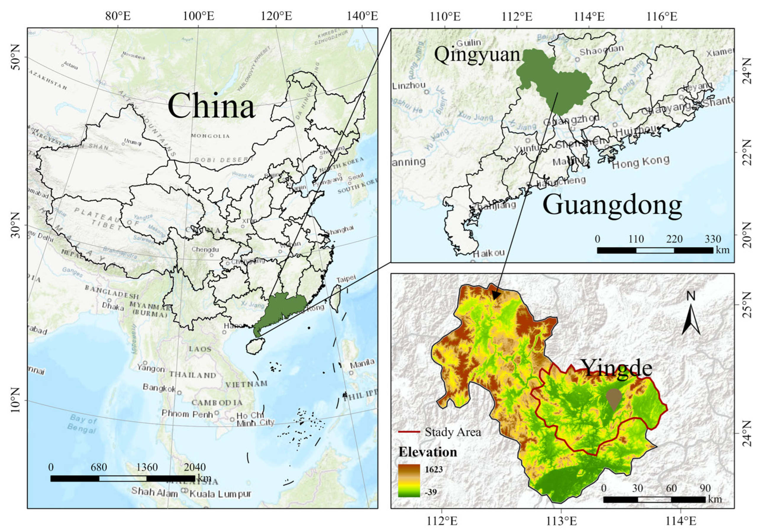
Figure 2 depicts the selected study location, which is located in Huihe Agricultural Tea Garden on Yunsha Road in Yinghong Town, Yingde City (Geographical coordinates: 23°50′31″ N–24°33′11″ N, 112°45′15″ E–113°55′38″ E), Qingyuan City, Guangdong Province, China. The tea garden is situated in an area with a warm and humid environment and good soil, ideal for the growth of large-leaved tea trees. Because the Tea red scab pathogen prefers temperatures of 16–23 °C and relative humidity of more than 80%, with a proclivity to break out in low temperatures and high humidity, samples were collected in the chosen tea plantation after 20 days of continuous rainfall in May 2024.

The samples obtained in this experiment were classified as Tea red scab illness grades with reference to Hunan Provincial Agricultural Technical Regulations HNZ205-2018. In order to limit the influence of leaf size on disease grade judgment, the data were merged and classified into three categories based on spot density D on each diseased leaf: mild, moderate, or severe. Equation (1) depicts the mathematical procedure for defining illness spot density.

$$D={\displaystyle \frac{N}{S}}$$

(1)

where N is the number of diseased spots in units of per, Manual counting; S is the leaf area in cm², which can be acquired using image segmentation; and D is the diseased spot density in units of per/cm².

The total number of valid samples acquired after screening the samples is 1188, with the training and test sets divided in a 7:3 ratio.

Table 1. Classification criteria and number of samples of Tea red scab.

Disease Level	Health	Mild	Moderate	Severe
Lesion density	0	D ≤ 0.75	0.75 ≤ D ≤ 1.5	D ≥ 1.5
Sample quantity	285	289	293	321

shows the samples’ exact division criteria as well as the number of samples in each group.

Wipe the collected tea leaves with paper towels to remove surface moisture and dust before capturing images. During the acquisition of RGB images of tea leaves affected by Tea red scab, an OPPO Reno Ace mobile phone was used for image capture. To minimize the influence of complex backgrounds on recognition accuracy, the diseased leaves were affixed onto white cardstock prior to photography. Mount the phone horizontally and position it 10–20 cm away from the target leaf during filming. Use a fixed light source to maintain consistent illumination. All images were saved in JPG format with a resolution of 3456 × 4608 pixels.

The hyperspectral acquisition system (Brand: Shuangli Hespec; Manufacturing Location: Jiangsu; Instrument Model: Gaia Field; Wavelength range: 400–1000 nm; Resolution: 3.8 nm; Number of optical channels: 256; Field of view: 19.8°; Frame rate: 15 fps) for this study is shown in Figure 3. To decrease instrumental interference, the hyperspectral pictures were calibrated in black and white in the software SpecView using Equation (2), which eliminated instrument errors. (After collecting tea leaf samples, first capture RGB images, then immediately proceed to hyperspectral imaging.)

$$R_{ref}={\displaystyle \frac{D{N}_{raw}-D{N}_{dc}}{D{N}_{white}-D{N}_{dc}}}$$

(2)

Following calibration of the hyperspectral pictures acquired for each sample, the appropriate Region of Interest (ROI) was chosen to obtain spectral curves with characterisation capacity. The ROI selection in this study covers the entire leaf area.

2.2. RGB Image Processing Methods and Model Construction

2.2.1. RGB Image Preprocessing

Image enhancement refers to the processing of degraded image features—such as edges, contours, and contrast—using specific techniques to improve visual quality, thereby converting images into a format more suitable for human interpretation or computational analysis [21]. In the context of agricultural disease detection, such techniques help suppress environmental noise, highlight lesion characteristics, and compensate for imaging deficiencies, thereby providing high-quality input data for subsequent classification models [22].

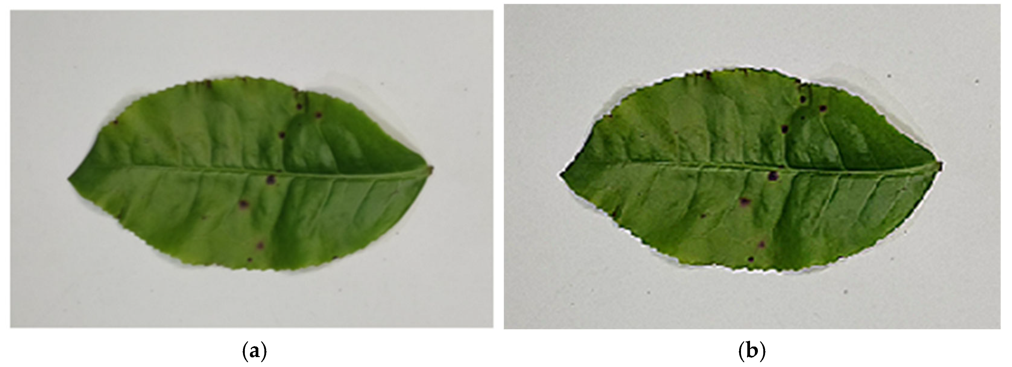
During the image preprocessing stage for Tea red scab, Laplacian sharpening filtering was employed to enhance the clarity of lesion edges and improve overall image quality. The effect of sharpening is demonstrated in Figure 4, which shows that the processed images display sharper lesion margins and more distinct features.

2.2.2. Classification Modelling Methods

Prior to the introduction of the AlexNet network, tasks such as image classification, segmentation, and recognition primarily relied on handcrafted feature extraction or combinations of traditional machine learning methods [23]. However, the process of manual feature design was often cumbersome, and even with machine learning-based classification, the overall robustness of the algorithm remained limited. The proposal of AlexNet fundamentally transformed this landscape, significantly advancing the application of deep learning in image processing and attracting widespread scholarly interest in related research.

Owing to its exceptional architecture and performance, AlexNet has been widely adopted in various computer vision tasks, including image classification and object detection [24]. Its breakthrough performance in the ImageNet Large Scale Visual Recognition Challenge (ILSVRC) established it as one of the benchmark models in the field of image classification, enabling high-accuracy categorization of a vast number of natural images [25]. The AlexNet architecture used in this study is illustrated in Figure 5. It consists of five convolutional layers and three fully connected layers. Each convolutional layer is equipped with convolutional kernels, bias terms, ReLU activation functions, and local response normalization (LRN) modules. The first, second, and fifth convolutional layers are each followed by a max-pooling layer, while the last three layers are fully connected. The final output layer utilizes a Softmax function to convert the network outputs into class probabilities, thereby enabling predictive classification of images. AlexNet achieved breakthrough performance in image classification tasks by leveraging a series of innovative techniques, including a deep architecture, the ReLU activation function, local response normalization, Dropout regularization, overlapping pooling, data augmentation, and multi-GPU training [26].

VGG16 is a deep convolutional neural network architecture developed by the Visual Geometry Group at the University of Oxford. It has been widely adopted in tasks such as image classification, object detection, and semantic segmentation [27]. The network is characterized by its uniform and symmetric structure, constructed through repeated blocks of convolutional layers with 3 × 3 kernels and pooling layers with 2 × 2 windows.

As illustrated in Figure 6, the input to the network is a color image of size 224 × 224 × 3. The initial convolutional layer employs 3 × 3 filters with a stride of 1, followed by ReLU activation, resulting in a feature map of size 224 × 224 × 64. After max pooling, the spatial dimensions are reduced to 112 × 112 × 64. This is followed by two convolutional layers with 128 channels of 3 × 3 kernels and ReLU activation, yielding outputs of size 112 × 112 × 128. Subsequent max pooling further reduces the size to 56 × 56 × 128. The network continues with two sets of convolutional layers: first, two layers with 256 channels, then two layers with 512 channels, each followed by max pooling. After processing through three convolutional layers with 512 filters and ReLU, the feature map size becomes 14 × 14 × 512. Another max pooling operation reduces it to 7 × 7 × 512. The 7 × 7 × 512 feature maps are then flattened into a vector and passed through two fully connected layers, each with 4096 units, followed by a final fully connected layer with 4 units. A Softmax classifier is applied at the output layer to produce predictions across the four target classes.

VGG16 employs a deep 16-layer architecture to construct a powerful hierarchical feature abstraction capability through successive nonlinear transformations. Its core design consists of repeatedly stacking small 3 × 3 convolutional kernels. This strategy increases network depth while expanding the effective receptive field via multi-layer cascading, thereby enabling comprehensive global feature representation [28]. Compared to larger convolutional kernels, this design reduces parameter complexity while enhancing the model’s nonlinear expressive capacity, effectively mitigating the gradient degradation problem in deep networks. However, the fully connected layers contribute a high parameter count, which increases computational cost and limits the model’s applicability in resource-constrained scenarios. Nevertheless, VGG16 establishes a standard for deep network design through its balanced and regular structure—systematically halving feature map dimensions while doubling channel depth at each stage—providing an important reference for the development of more efficient architectures in subsequent research.

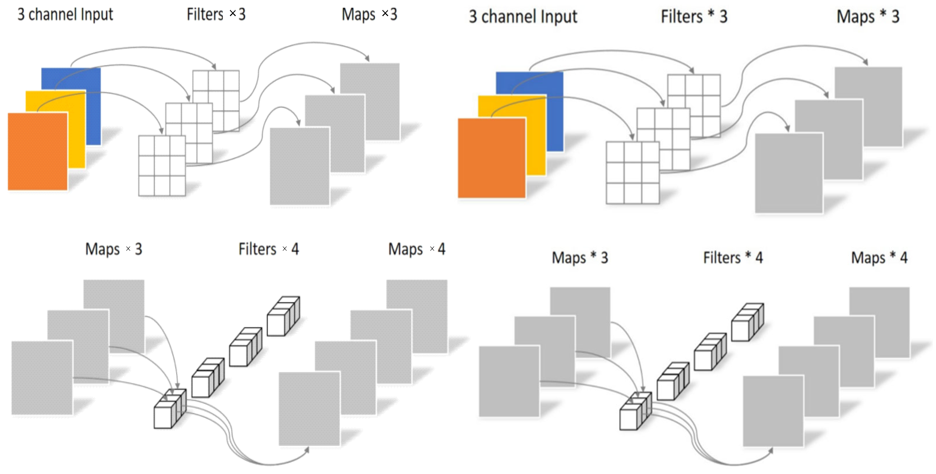
As depicted in Figure 7, MobileNet-V1 utilizes depthwise separable convolutions, which decompose a standard convolution into two independent layers: a depthwise convolution and a pointwise convolution. The depthwise convolution applies a spatial filter to each input channel individually, preserving channel isolation. The pointwise convolution then follows, employing a 1 × 1 kernel to project the output of the depthwise convolution into a new channel space. This step facilitates cross-channel feature fusion and enables dimensionality reduction [29].

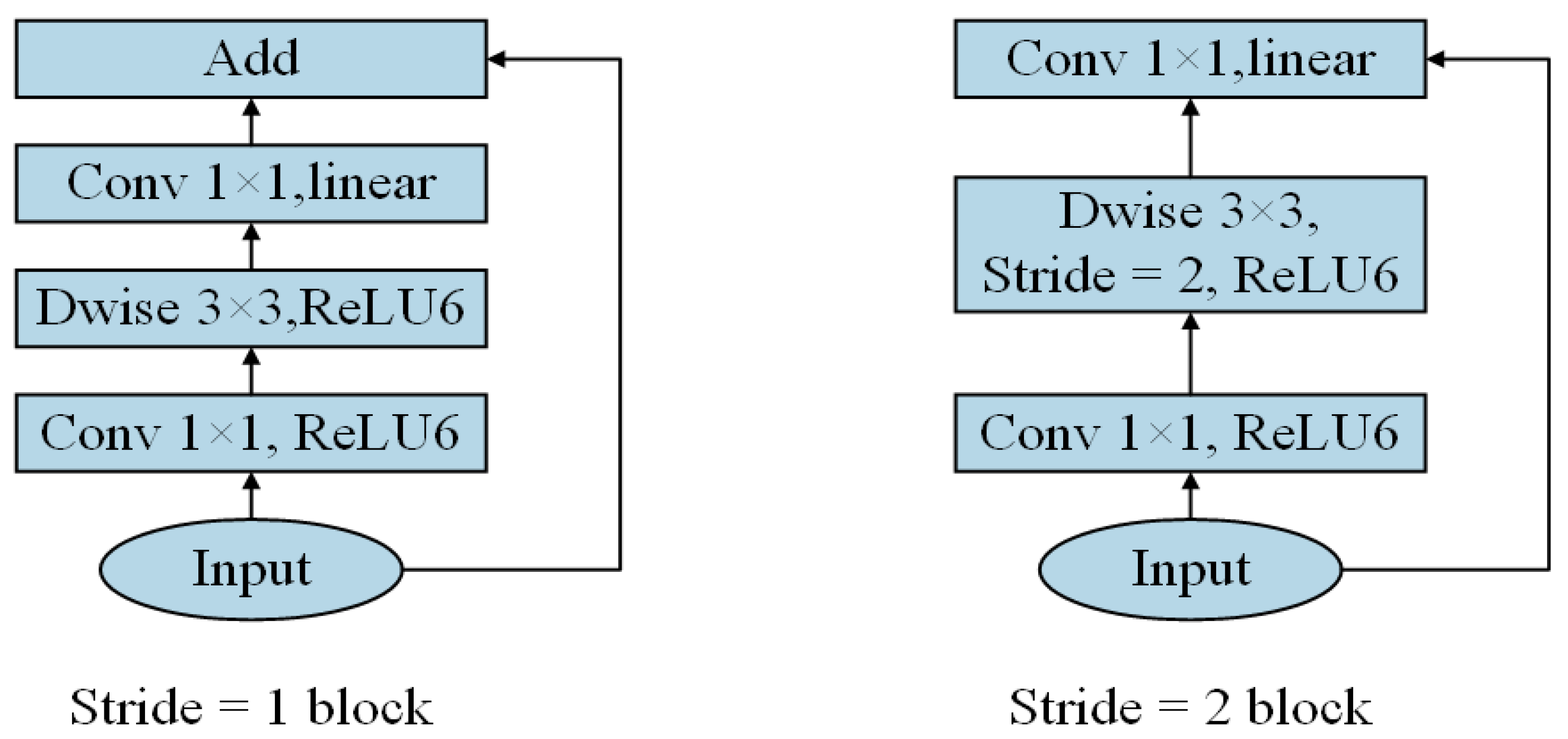
MobileNet-V2 is a lightweight deep convolutional neural network architecture specifically designed for mobile and embedded devices, enabling efficient image classification and other vision tasks under constrained computational resources. Evolved from MobileNet-V1, this enhanced version introduces two key innovations: inverted residual structures and linear bottleneck layers. These contributions achieve a breakthrough in balancing computational efficiency and feature representation capability [30]. The inverted residual architecture differs from the traditional residual module’s “dimension reduction followed by dimension expansion” channel processing pattern. As shown in Figure 8, it first expands the low-dimensional input channels by a factor of 6 through 1 × 1 convolutions, then extracts spatial features via 3 × 3 depth convolutions, and finally compresses the channel dimensions using linear 1 × 1 convolutions [31]. This architecture creates a high-dimensional feature space in the intermediate layer, effectively mitigating feature information loss caused by channel reduction in deep separable convolutions. To address the irreversible damage to low-dimensional features caused by the ReLU activation function in the linear bottleneck layer, a linear activation replaces the nonlinear transformation at the end of the bottleneck layer, preventing gradient vanishing due to dimensional collapse. Experiments demonstrate that these enhancements enable MobileNet-V2 to achieve a 4.3% improvement over MobileNet-V1 under equivalent computational cost on the ImageNet dataset, validating the feasibility of achieving accuracy breakthroughs through structural innovation in lightweight networks.

2.3. Hyperspectral Image Preprocessing Methods and Model Construction

2.3.1. Spectral Signal Preprocessing

Owing to the hyperspectral camera’s hardware features, the obtained hyperspectral data have high-frequency noise, systematic bias, and scaling effects, and such data readily interfere with the modelling effect when utilized directly for modelling [32]. As a result, spectral data must be pre-processed before analysis in order to increase the quality of modelling data [33]. Multiplicative Scatter Correction (MSC) is a technique for correcting the influence of scattering in spectral data that is appropriate for the processing of solid and powder materials [34]. Standard Normal Variate Transformation (SNV) is a popular spectral preprocessing approach for removing systematic bias and scaling effects in spectral data [35]. The objective is to convert raw spectral data into standard normally distributed variables, allowing the data to preserve chemical information while eliminating interference from non-chemical sources, hence improving data stability. Savitzky-Golay (SG) filtering is a digital signal processing method used to smooth out signals [36]. First Derivative (FD) processing is a popular signal processing approach that shows the rate of change in spectral reflectance as a function of wavelength, highlighting absorption peaks and valleys and aiding in the identification of subtle features in the spectrum [37]. In this study, four preprocessing methods, namely multivariate scattering correction, standard normal variable transformation, Savitzky-Golay filtering, and first-order derivative transformation, are chosen to investigate the effects of different methods on the spectral curves and to prefer a combination of preprocessing methods suitable for the current algorithmic dataset.

2.3.2. Classification Models and Optimisation Algorithms

Hyperspectral data, with hundreds of continuous bands and nanometre resolution, can catch delicate properties of materials. However, it is high-dimensional and contains redundant information. End-to-end learning allows deep learning models to immediately extract features and classification rules, eliminating the multi-step error accumulation of previous methods and enhancing classification accuracy and efficiency.

One-Dimensional Convolutional Neural Network

One-dimensional Convolutional Neural Network (1D-CNN) is a type of Convolutional Neural Network (CNN) that is particularly effective at processing time series data, text, and one-dimensional signals. 1D-CNN uses a convolutional layer to extract local patterns in sequential data, allowing for better interpretation and processing. 1D-CNN operates on the premise of extracting and combining features in sequential data using convolutional techniques and nonlinear activation functions [38]. 1D-CNN employs a convolution kernel to execute a sliding convolution operation on the input sequence in order to generate a new series of features. To capture characteristics at different scales, the convolution kernel’s size and step size can be modified accordingly [39].

The benefits of 1D-CNN include its ability to automatically learn useful feature representations from one-dimensional data, and because of the parameter-sharing mechanism of the convolutional layer, 1D-CNN is more efficient in terms of parameter count than fully connected-layer networks, making it better suited to dealing with long sequential data. However, 1D-CNN has significant limits; for particularly lengthy sequences, more layers may be required to capture long-term dependencies, making model training more challenging.

Gate Recurrent Unit

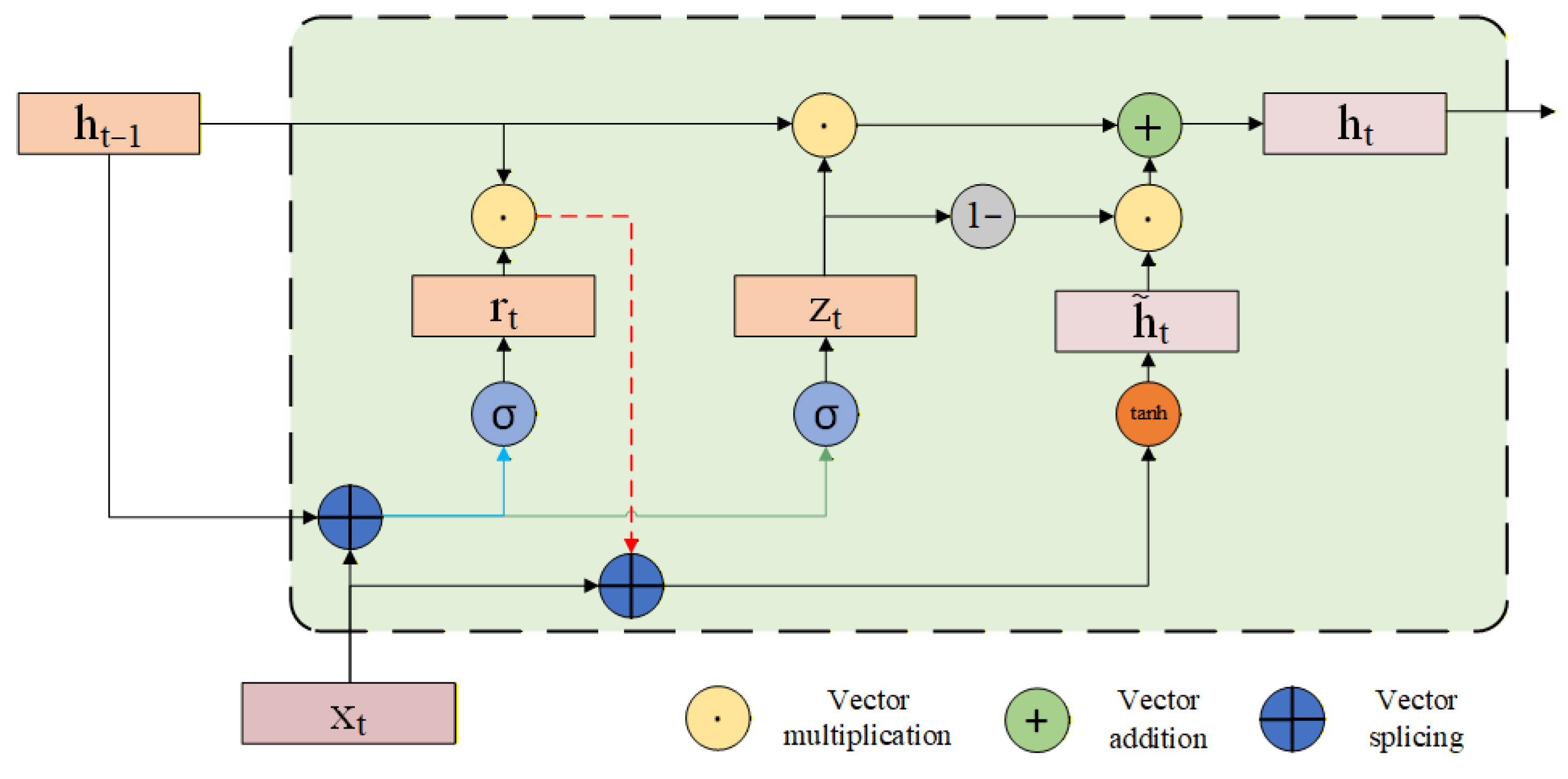
The Gate Recurrent Unit (GRU) architecture is a sort of Recurrent Neural Network (RNN) that seeks to address the issue of gradient vanishing and explosion that regular Recurrent Neural Networks (RNNs) encounter when dealing with sequential input [40]. GRU regulates information flow by introducing three gating mechanisms: Update Gate, Reset Gate, and Output Gate, which improve the ability to capture long-term dependencies [41]. The update gate uses a sigmoid activation function to generate a value between 0 and 1 that controls how much the current state is updated by combining new information with the prior state. The reset gate, which creates a value using the sigmoid activation function, controls how much information from the previous state should be ignored, preventing gradient explosion and allowing the network to better capture long-term dependencies. The output gate determines which part of the state is sent to the output, and its value is determined by the sigmoid function.

Figure 9 depicts the GRU network structure, with $r_t$ as the reset gate, $z_t$ as the update gate, $h_{t-1}$ as the last output of the prior position, $x_t$ as the current position input, $h_t$ as the updated value as the alternative output at the present moment.

Equations (3) and (4) contain the formulas for reset gate $r_t$ and update gate $z_t$. The output values range from 0 to 1 for selecting the information left behind and forgotten after the current position input $x_t$ and the output $h_{t-1}$ of the previous position’s hidden layer are summed together after a linear change in the activation function. Where $W_r$ and $b_r$ signify the reset gate’s weight matrix and bias vector, and $W_Z$ and $b_Z$ denote the update gate’s weight matrix and bias vector.

$$r_t=\sigma \left(W_r{x}_t+U_r{h}_{t-1}+b_r\right)$$

(3)

$$Z_t=\sigma \left(W_Z{x}_t+U_Z{h}_{t-1}+b_Z\right)$$

(4)

Equation (5) is the formula for computing the candidate value following an update to ${\tilde{h}}_t$. It is decided by the reset gate $r_t$, the previous position’s output $h_{t-1}$, and the current position’s input $x_t$, all of which need be supplied to the control in order to calculate the current state.

$${\tilde{h}}_t=\tanh \left(W_c{x}_t,U\left(r_t·h_{t-1}\right)\right)$$

(5)

Equation (6) demonstrates that the current position’s ultimate output is $h_t$, which is decided by the updated candidate value ${\tilde{h}}_t$, the update gate $Z_t$, and the prior position’s input $h_{t-1}$. Because the value of $Z_t$ ranges from 0 to 1, the final output $Z_t$ has more information in ${\tilde{h}}_t$ as $Z_t$ approaches 0, and $h_t$ contains more information in $h_{t-1}$ as $Z_t$ approaches 1.

$$h_t=z_t·h_{t-1}+\left(1-z_t\right)·{\tilde{h}}_t$$

(6)

GRU’s workflow includes receiving the current input and prior state, computing the gating signal, updating the state, computing the output, sending the updated state to the next time step, and repeating the process. GRU’s advantages include its capacity to efficiently capture long-term dependencies in sequential data, alleviate the gradient problem, and adapt to various types of sequential data and workloads [42]. GRUs have been widely employed in natural language processing, speech recognition, time series prediction, and other sectors, with successful results [43].

2.3.3. Newton-Raphson-Based Optimizer

The Newton-Raphson-based optimizer (NRBO) is a revolutionary metaheuristic algorithm. It starts the search for the best solution by creating an initial random population within the limits of the candidate solutions, and it has powerful global and local optimisation capabilities [44]. The NRBO algorithm is modeled after the Newton-Raphson method and employs two rules to investigate the entire search process: the Newton-Raphson Search Rule (NRSR) and the Trap Avoidance Operator (TAO) [45,46]. Where NRSR employs the Newton-Raphson method with Taylor series expansion to control the vectors in order to more accurately explore the feasible region and achieve better locations, and the parameters whose positions x are next to one another are designated as x + NRSR vs. x − NRSR. Because the NRSR rule is the main component of NRBO, when using the population-based search technique, the convergence of the parameter search is expressed as Equation (7).

$$NRSR=random\times {\displaystyle \frac{\left(X_{\omega }-X_b\right)\times \Delta x}{2\times \left(X_{\omega }+X_b-2\times x_n\right)}}$$

(7)

where random denotes a normally distributed random number with mean 0 and variance 1, $X_{\omega }$ represents the worst location and X_b represents the best position. The parameters optimized by the NRSR search algorithm can be written as Equations (8) and (9).

$$x_n^{IT+1}=r_1\times \left(r_1\times X{1}_n^{IT}+\left(1-r_1\right)\times X{2}_n^{IT}\right)+\left(1-r_1\right)\times X{3}_n^{IT}$$

(8)

$$X{3}_n^{IT}=X{1}_n^{IT}-\delta \times \left(X{2}_n^{IT}-X{1}_n^{IT}\right)$$

(9)

where $r_1$ is a random number, $X{1}_n^{IT}$, $X{2}_n^{IT}$, and $X{3}_n^{IT}$ represent the most recent vector coordinates discovered during the exploration process. At the same time, an adaptive parameter $\delta$ is added to change the direction of iteration, and the iterative process is continued until the required precision is met or the maximum number of iterations is reached.

$$\delta ={\left(1-\left({\displaystyle \frac{2\times IT}{Max\_IT}}\right)\right)}^5$$

(10)

Equation (10) depicts the calculation of $\delta$. IT is the current number of iterations, whereas Max_IT denotes the maximum number of iterations, and the value of $\delta$ ranges between (−1, 1) according to Equation (10).

The use of second-order derivatives for convergence in the NRSR iteration process causes the ideal parameters to quickly fall into local optimal solutions. Furthermore, the trap operator TAO can improve the NRBO algorithm’s effectiveness in dealing with real-world problems and adjust the position of the vectors after each iteration of the NRSR algorithm. Equation (11) guides the parameter iteration, causing the final result to deviate from local convergence and avoid the local optimal solution.

$$X_{TAO}^{IT}=\left\{\begin{array}{l}{X}_n^{IT+1}+{\theta }_1\times \left({\mu }_1\times X_b-{\mu }_2\times X_n^{IT}\right)+{\theta }_2\times \delta \\ \times \left({\mu }_1\times Mean\left(X^{IT}\right)-{\mu }_2\times X_n^{IT}\right),{\mu }_1<0.5\\ X_b+{\theta }_1\times \left({\mu }_1\times X_b-{\mu }_2\times X_n^{IT}\right)+{\theta }_2\times \delta \\ \times \left({\mu }_1\times Mean\left(X^{IT}\right)-{\mu }_2\times X_n^{IT}\right),\mathrm{otherwise}\end{array}\right.$$

(11)

where ${\theta }_1$ and ${\theta }_2$ are random numbers ranging from (−1, 1) to (−0.5, 0.5), ${\mu }_1$ and ${\mu }_2$ are random parameters, $X_n^{IT}$ is the current vector’s position, and $X_n^{IT+1}$ is the position of the new vector in the next iteration. The NRBO parameter optimisation algorithm improves the exploration ability of NRBO by NRSR by using first-order and second-order derivatives to accelerate the updating of the parameter positions, as well as the convergence speed to reach the improved search space position; and increases the stochasticity and diversity of the solution by the TAO operator to help the algorithm avoid falling into local optimal solutions [47]. The NRBO method gradually optimises the model parameters across multiple rounds. In each iteration, the algorithm examines the performance of the existing parameter settings and adjusts them in accordance with the natural rhythm strategy in order to find better solutions.

2.3.4. Model Construction

In this study, a total of 1188 samples from the dataset were separated into training and test sets in a 7:3 ratio, for the gathered spectrum dataset of Tea red scab disease ratings. Monte Carlo cross-validation was employed, with 100 iterations run to obtain the average result. Disease rank discrimination was carried out utilizing 1D-CNN, GRU, CNN-GRU, and NRBO-CNN-GRU.

The approach for using the NRBO-CNN-GRU model proposed in this work is as follows. First, spectrally sensitive bands are retrieved using 1D-CNN, which has two layers of convolution with 16 and 32 kernels of 3 × 1 size and a step size of 1. Following each convolution layer, a 2 × 1 maximum pooling layer with a step size of 2 is used to maintain the most important feature information. Following that, the output of each node is normalized using a Batch Normalization layer (BNL). By applying batch normalization layers, the input data to the subsequent network layers becomes more stable, thereby accelerating the training process [48]. Following preprocessing with the SNV-SG-FD method, the hyperspectral data of diseased leaves were fed into the model. An initial convolutional layer employing sixteen 3 × 1 kernels performed preliminary feature extraction. These features were subsequently passed to a second convolutional layer with thirty-two 3 × 1 kernels to abstract higher-level representations. Finally, the output was directed through a Dropout layer to mitigate overfitting, thereby preparing the features for subsequent processing by the GRU layer. Finally, a ReLU activation layer is added to improve the network’s nonlinear fitting ability. After the CNN processes the data, the resulting features are tiled as one-dimensional vectors and fed onto the GRU layer. In this research, two layers of GRU are employed. The first layer has 128 hidden units and efficiently captures the dynamic change pattern of illness features in the temporal dimension using its unique update gate and reset gate mechanism. To prevent the model from overfitting, a Dropout regularisation layer is inserted between the two GRU layers, with a neuron dropout rate of 0.5.

The second GRU layer employs 64 hidden units for feature refining, and its output is sent into the fully connected classifier after global average pooling. The last fully connected layer defines the Softmax activation function, with the number of output nodes corresponding to the samples’ four classes. The CNN excels at extracting local features, whereas the GRU can capture long-term dependencies in sequential data and address gradient vanishing. The CNN-GRU composite network structure employed in this paper is seen in Figure 10. Combining the benefits of these two methods, the network minimizes the number of parameters and the risk of overfitting, improving detection accuracy and network performance while also improving training efficiency. Finally, the NRBO algorithm is utilized to optimize three important CNN-GRU model parameters: the number of hidden layer nodes, the learning rate, and the regularization factor.

Table 2. Optimal parameter range for the NRBO optimization model.

Parameter	Set Value
MiniBatchSize	128
Range of L2 Regularization Coefficient	[1 × 10−4, 1 × 10−1]
Number of hidden nodes range	[10, 30]
Learning rate range	[1 × 10−3, 1 × 10−2]
Epoch	100
Maximum number of iterations	10

shows the parameters of NRBO.

The conditions for processing data in this study are as follows: Hardware processor: AMD Ryzen 7 5800H with Radeon Graphics @3.20 GHz; Memory: 8 GB; Software environment: CUDA Toolkit 10.1; CUDA NUCLEUS V7.6.0; MATLAB R2023b; Python 3.8; PyTorch-GPU 1.6.0; Operating system version: Windows 11.

2.4. Model Evaluation

Four criteria were utilized to assess the performance and effectiveness of each classification model: accuracy, precision, recall, and the F₁-score. The exact calculation of each value is as follows: TP denotes the number of samples correctly predicted as positive categories, FP the number of samples incorrectly predicted as positive categories, TN the number of samples correctly predicted as negative categories, and FN the number of samples incorrectly predicted as negative categories.

$$Accuracy={\displaystyle \frac{TP+TN}{TP+TN+FP+FN}}$$

(12)

$$Precision={\displaystyle \frac{TP}{TP+FP}}$$

(13)

$$Recall={\displaystyle \frac{TP}{TP+FN}}$$

(14)

$$F_1-score={\displaystyle \frac{2\times Precision\times Recall}{Precision+Recall}}$$

(15)

The accuracy rate is calculated as the ratio of all correctly classified samples to the total number of samples, which includes both positive and negative categories. The precision rate which is the ratio of samples properly recognized as positive classes to total positive class samples. It is used to assess the accuracy of forecasting positive classes. The recall rate is the proportion of samples properly predicted by the model to be in the positive category out of all samples that are really in the positive category. The F₁-score is the reconciled mean of accuracy and recall; a high model score suggests a good balance between precision and memory, implying an accurate and complete model.

3. Results

3.1. RGB Image Model Results

The AlexNet, MobileNet-V2, and VGG16 models, all trained on RGB images, achieved classification accuracies below 80%. A comparative analysis of these architectures reveals that structural differences among the networks significantly influence their overall performance in the classification task.

According to

Table 3. Performance of different models.

Modelling Methods	Accuracy	Precision	Recall	F1-Score
AlexNet	63.48%	63.77%	64.23%	63.75%
MobileNet-V2	79.26%	79.15%	78.95%	78.73%
VGG16	65.73%	71.50%	65.18%	65.99%

, as an early representative of deep models, AlexNet achieved an accuracy of 63.48% and an F₁-score of 63.75%, indicating limitations in its feature abstraction capacity. This can be attributed to its relatively shallow convolutional architecture and the use of large 11 × 11 kernels. Although large convolutional kernels facilitate the capture of global features, they also increase sensitivity to high-frequency noise and introduce parameter redundancy, thereby constraining the model’s discriminative ability for complex textures. In contrast, MobileNet-V2 achieves an accuracy of 79.26% and an F₁-score of 78.73% through synergistic optimization of inverted residual structures and depthwise separable convolutions. Its lightweight design incorporates channel expansion to mitigate information loss in low-dimensional features, while linear bottleneck layers reduce feature distortion caused by excessive nonlinear activation. These innovations enable the model to maintain high robustness with significantly reduced parameters. VGG16 performs intermediately between AlexNet and MobileNet-V2, with an accuracy of 65.73% and an F₁-score of 65.99%. Although it shows clear improvement over AlexNet, its results remain lower than those of MobileNet-V2.

3.2. Sample Hyperspectral Curve and Pre-Processing Results

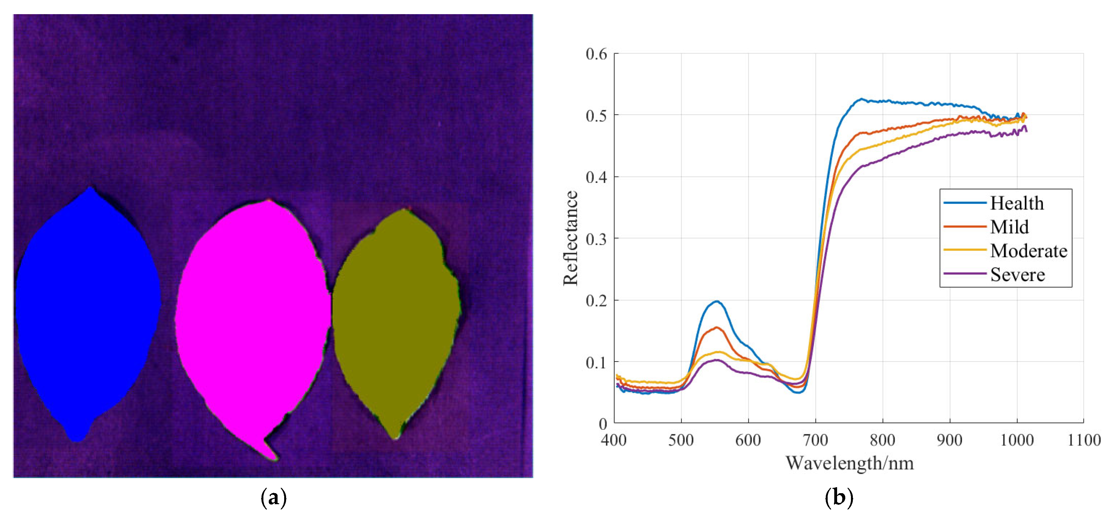
Figure 11 depicts the usage of leaf-averaged spectra to represent each sample. The general trend of leaf mean spectral reflectance across various Tea red scab disease classes was consistent and increased with disease class. The four disease classes’ reflectance increased in the wavelength range of 401–548 nm, decreased in the wavelength range of 548–683 nm, and increased exponentially in the wavelength range of 683–770 nm.

The spectral data after different pre-processing were compared with the non-preprocessed spectral data, and the spectral data obtained after different pre-processing of the original spectra were input into a 1D-CNN network for classification modelling. The effect of different pre-processing methods on the classification effect of spectra was judged by the classification accuracies of each model’s training and test sets. The results of the comparison of pre-processing methods are shown in

Table 4. Test set accuracy of 1D-CNN models with different preprocessing methods.

Ordinal Number	MSC	SNV	SG-FD	Accuracy
1				84.58%
2	√			85.74%
3		√		85.46%
4			√	85.91%
5	√		√	85.17%
6		√	√	86.83%
7	√	√		84.66%
8	√	√	√	84.86%

.

Model 1’s accuracy without preprocessing was 84.58%, while the modelling effect of the data after preprocessing was improved to varying degrees. Model 2 is preprocessed with MSC, which corrects the baseline shift caused by scattering effects, and the accuracy improves by 1.16%, showing that scattering interference exists in the tea-round ruddy star disease spectral data gathered in this study. Model 3 is preprocessed with SNV, which eliminates the global intensity difference and increases model accuracy by 0.88%; however, the effect is significantly weaker than that of MSC, indicating that scattering is the primary interference, followed by light-range difference. Model 4 employs SG + FD preprocessing, which improves feature contrast after smoothing spectral noise, and the model effect is increased by 1.33% with the best result, demonstrating the relevance of noise suppression and detailed feature amplification. As for the combination method, SNV-SG-FD has the best effect with 86.83% accuracy, which is due to the fact that after SNV eliminates the global intensity difference, SG-FD further suppresses the noise and strengthens the local features to form a synergistic effect; however, the effect of MSC-SG-FD decreases, which could be due to excessive feature elimination or amplification of the residual noise by the derivative processing after the MSC corrects the scattering base.

3.3. Performance Results of Different Network Models for Data Classification

To explore the effect of feature extraction methods in deep networks on classification model performance, CNN, GRU, CNN-GRU, and NRBO-CNN-GRU classification models were built using raw spectra (RAW) and spectra preprocessed with SNV-SG-FD, respectively. The classification model’s results are presented in

Table 5. Model effects of different modelling methods.

Datatypes	Modelling Methods	Accuracy	Precision	Recall	F1-Score
RAW	CNN	85.25%	85.30%	85.24%	85.16%
	GRU	84.24%	84.51%	84.21%	83.87%
	CNN-GRU	88.96%	88.58%	88.95%	88.74%
	NRBO-CNN-GRU	91.74%	91.79%	91.76%	91.73%
SNV-SG-FD	CNN	86.83%	87.04%	86.82%	86.74%
	GRU	86.36%	87.16%	86.34%	86.15%
	CNN-GRU	90.23%	90.79%	90.21%	90.32%
	NRBO-CNN-GRU	92.43%	92.51%	92.42%	92.43%

.

To begin, regardless of whether preprocessing is conducted, all models perform better after SNV-SG-FD preprocessing, demonstrating the importance of data preprocessing. The CNN model, for example, raised its accuracy from 85.25% of the raw data to 86.83%, while the F₁-score increased from 85.16% to 86.74%. The GRU model’s accuracy increased by 2.12% and the F₁-score increased by 2.28%. This improvement is primarily due to more regular data distribution after preprocessing, which reduces the learning complexity of the model, particularly for the CNN model that depends on local feature extraction, which shows the greatest benefit. The CNN-GRU model demonstrated significant feature extraction capacity in the raw data, with an accuracy of 88.96%. Its accuracy improves to 90.23% after preprocessing, demonstrating that the synergistic effect of preprocessing and hybrid architecture may overcome the limitations of a single model. When employing CNN and GRU algorithms to predict the original spectrum and the preprocessed spectrum, the difference is clear. While the difference between the evaluation indexes of the original and preprocessed spectral models when modelled by CNN-GRU is minor, the recall and F₁-score evaluation indexes are higher than those of CNN and GRU. This shows that CNN-GRU can effectively withstand interference generated by external factors and has good anti-interference and stability capabilities.

In raw data, CNN-GRU outperforms CNN and GRU with 88.96% accuracy, representing a 4.35% and 5.60% increase, respectively. This is due to the combination of CNN’s local feature extraction and GRU’s sequence modeling capabilities. CNN uses convolution kernels to capture spatial patterns such as absorption peak and valley patterns in the spectrum, whereas GRU models long-range temporal relationships between bands, and the two can be combined. The combination of the two can capture both static local properties and dynamic global changes. CNN marginally beats GRU in a single model, with a 1.01% accuracy difference. After SNV-SG-FD preprocessing, CNN-GRU dominates with an accuracy of 90.23%, up 3.40% and 3.87% from single CNN and GRU, respectively, demonstrating the superiority of the CNN-GRU method. The difference between CNN and GRU expands by 0.47% after preprocessing, demonstrating that normalization and feature enhancement are better suited to spatial feature extraction. And while GRU outperforms CNN in precision rate, its recall rate remains low, demonstrating that it is sensitive to the consistency of global distribution yet has limits in complicated feature capture.

Further study of the model metrics reveals that the difference between the F1 score and the accuracy of all models is less than 0.40%, indicating that the classification results’ precision and recall are more balanced and free of substantial skewness. GRU has the best precision rate of the three after preprocessing, but its recall rate is somewhat lower than CNN’s, indicating that it excels at controlling false alarms but fails to recognize some positive cases. CNN-GRU outperforms in the balance test, and its preprocessed F1 score nearly coincides with the accuracy rate, demonstrating that the hybrid architecture can maintain high precision while efficiently minimizing the risk of missed detection.

NRBO-CNN-GRU performs optimally on both types of data. On the raw data, NRBO increases CNN-GRU’s recall from 88.95% to 91.76%; on the preprocessed data, the difference between the accuracy and recall of NRBO-CNN-GRU is less, and the optimised model achieves a better balance between misdetections and leakage detections. The results reveal that the NRBO parameter optimisation approach efficiently modifies the model hyperparameters, improving the model’s adaptability to data distribution.

3.4. Analysis of Model Validity

As indicated by the results in Section 3.1 and Section 3.3, the NRBO-CNN-GRU model constructed based on hyperspectral images demonstrates superior performance in classifying the severity levels of tea leaf red spot disease. The effectiveness of the model is further analyzed below through its performance across different sample categories and via confusion matrices.

3.4.1. Comparison of Model Performance for Different Sample Categories

This study examines the classification performance of the models for each sample category to examine the gap in model effectiveness between different samples. Based on the performance of the CNN, GRU, CNN-GRU, and NRBO-CNN-GRU models in the four sample categories, it is possible to conclude that the models differ in their adaptability to each.

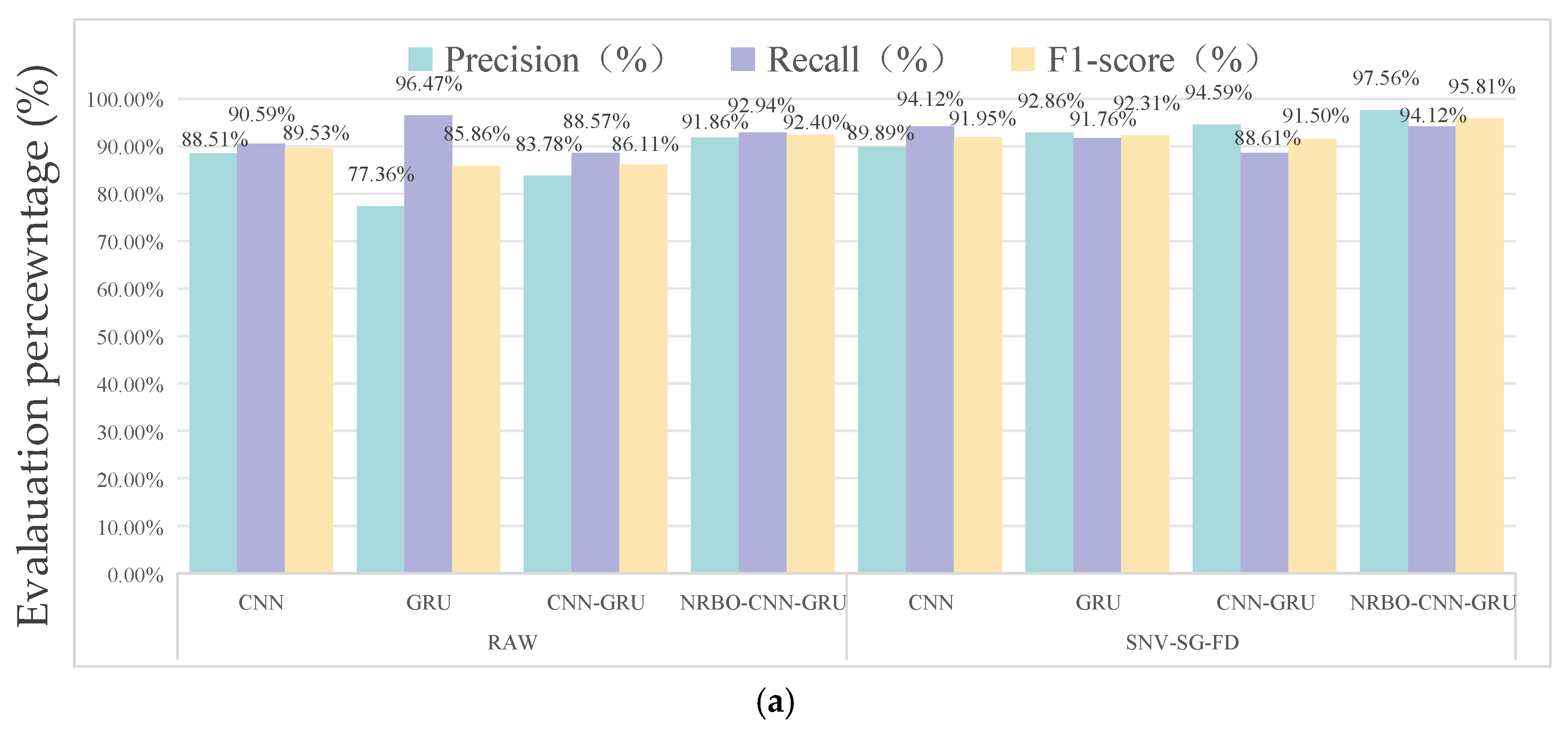
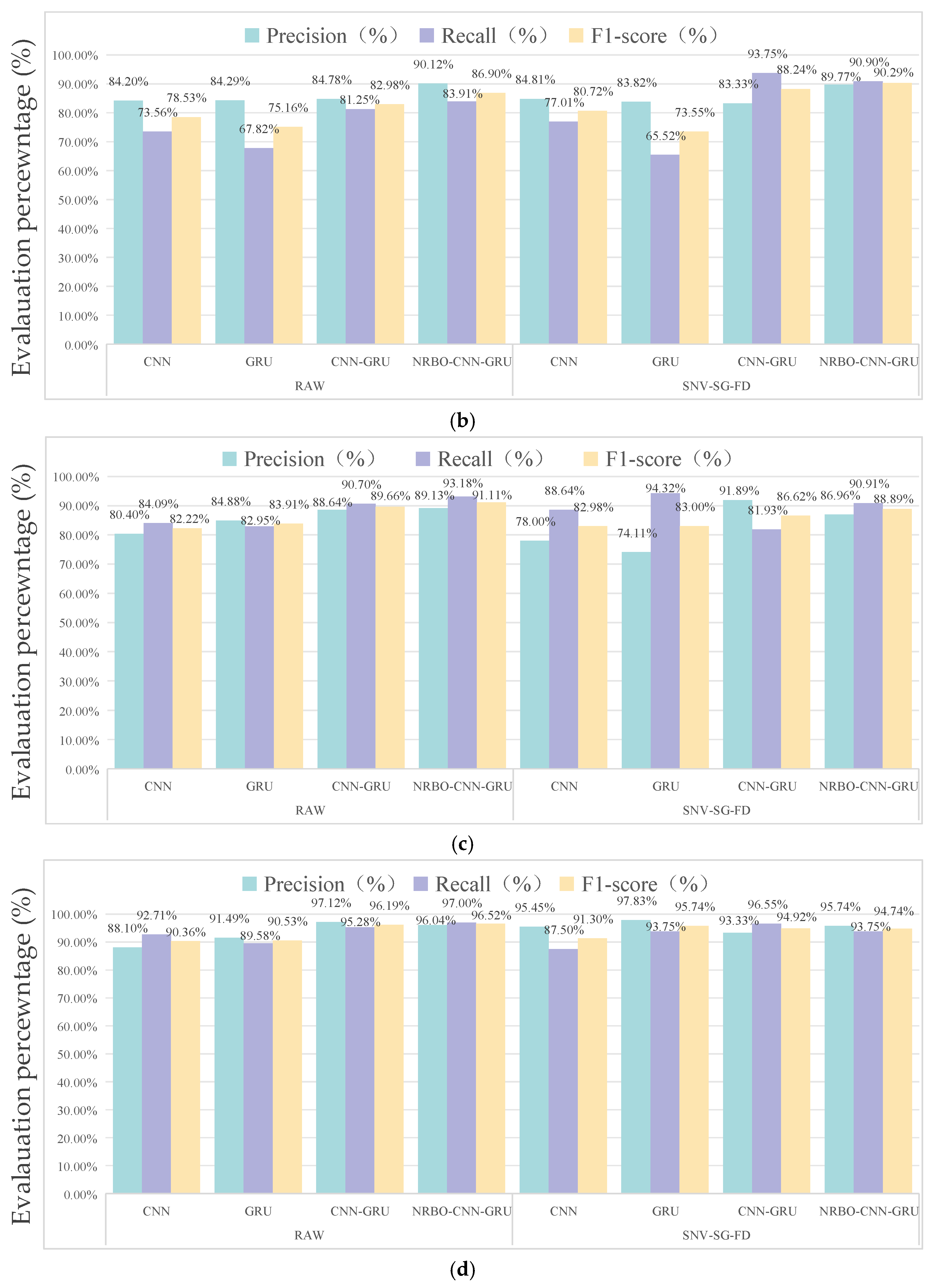
As demonstrated in Figure 12a, preprocessing greatly increases GRU model efficacy in healthy data, with the highest precision rate of 92.86% and an F₁-score of 92.31%. This is owing to the fact that GRU is more sensitive to long-term changes, which are more noticeable in healthy samples. CNN has the highest recall but a somewhat lower precision rate, indicating model instability. CNN-GRU has the best precision rate in this category at 94.59%, but its recall rate is significantly lower. The NRBO-CNN-GRU model outperforms the others in terms of post-processing performance improvement, with an F₁-score of 95.81%. The 94.12% recall and 97.56% precision rate suggest that parameter adjustment improves model stability to some extent. As shown in Figure 12b, CNN-GRU has a higher F₁-score of 88.24% in light samples compared to CNN (80.72%) and GRU (73.55%), indicating that the model can effectively capture the detailed features of the medium samples. However, the poor precision rate suggests that the spectral data in such samples is ambiguous or has an uneven distribution. GRU has the lowest recall rate in this category, at 65.52%, indicating that the sequence modelling is not sensitive enough to local detailed details.

As shown in Figure 12c, the GRU model for moderate samples tops the list with 94.32% recall, but 74.11% precision significantly lowers the F₁-score, whereas CNN-GRU achieves the optimal F₁-score by balancing precision and recall, indicating that the hybrid CNN-GRU architecture is more robust in this type of complex features. As shown in Figure 12d, the RAW + CNN-GRU model with heavy samples performs best with an F₁-score of 96.19%, and the performance of most of the models decreases after preprocessing, which could be due to the fact that SNV-SG-FD destroys detailed information in the spectral reflectance of heavy samples. The GRU performs the best, with a precision of 97.83% after preprocessing but a worse recall. Among the models, the GRU attained the optimal precision of 97.83% following preprocessing; however, this was accompanied by comparatively worse recall performance. The NRBO-optimized CNN-GRU model excels in handling large samples, as evidenced by its high recall rate of 97.00% when using raw spectral data, thereby minimizing the likelihood of missed detections. Nevertheless, the application of preprocessing leads to a decline in recall, attributable to the loss of pertinent spectral features during the preprocessing phase.

Overall, CNN is stable but does not perform exceptionally well; in a large sample with distinct features, GRU achieves the highest F₁-score of 95.74%, while precision and recall can reach 97.83% and 93.75%, respectively. This demonstrates its exceptional ability to simulate extremely consistent sequence patterns. The CNN-GRU model’s metrics results do not change considerably between healthy and heavy samples, and both are superior compared to the light and medium outcomes. This means that the healthy and hefty samples are of higher quality and easier to distinguish. While NRBO-CNN-GRU outperforms in light and medium samples with comparable features, with F₁-score of 90.29% and 88.89%, respectively. The advantage of resolving spectral features using local-global resolution suggests that the CNN-GRU model, with suitable hyperparameters, may learn the spectral differences between the two types of samples more effectively.

3.4.2. Confusion Matrix Analysis

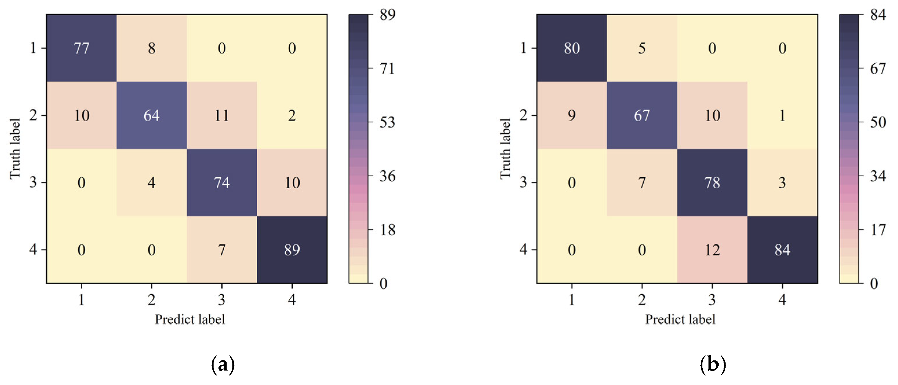
This study investigates the impact of preprocessing and modelling methods on model effectiveness by examining the classification effect of spectral data in various sample categories and comparing the model confusion matrices of the original and preprocessed spectra, as shown in Figure 13. The distribution of misclassified samples in the confusion matrix demonstrates that different models and preprocessing procedures perform significantly differently in the four-classification test. This distinction derives from the model architecture’s inherent features and is also directly tied to the data pretreatment technique.

Figure 13a depicts the effect of the RAW + CNN model, which causes mild samples to be misclassified as healthy and moderate samples, accounting for 24.13% of the total healthy samples. This is due to the ambiguity of mild samples in the feature space, which contain both healthy and moderate local features, making it difficult for the model to capture their uniqueness using a single convolution operation. Moderate samples, on the other hand, are misclassified as heavy by up to 11.36%, showing that the higher-order detailed features are not properly differentiated, and the model tends to identify boundary samples as heavy due to higher similarity. The preprocessed model helps to ease this issue to some extent. As illustrated in Figure 13b, Processing + CNN reduces the misclassification rate from moderate to heavy, implying that the preprocessing procedure improves the feature salience of moderate data. However, the increased likelihood of heavy being misinterpreted as moderate suggests that preprocessing reduces the essential properties of moderate samples, resulting in an overlap of the decision boundary between the two categories.

As illustrated in Figure 13c,d, the GRU model built with the raw data misclassifies moderate samples as healthy by up to 22.98%. This is because GRU relies heavily on time-series segments. Following preprocessing, the number of mild samples misclassified as moderate rose, accounting for 27.58% of the total number of mild samples. It implies that the SNV normalisation operation disrupts the link between the original temporal sequences, bringing the temporal segments of mild and moderate closer together in the normalized space. Figure 13e,f shows how the CNN-GRU fusion model lowers cross-category misclassification by merging local and temporal information. RAW + CNN-GRU decreases the number of moderate-to-severe samples from 10 to three in CNN. Following preprocessing, CNN-GRU reduces the number of samples with mild misclassification as moderate in CNN from 10 to 4. It is proved that SG efficiently lowers noise interference on healthy sample features, but the convolutional layer’s local features and GRU’s long-term dependencies can distinguish detail differences synergistically.

The NRBO parameter optimisation provides a clear advantage in terms of overall performance balancing. As illustrated in Figure 13g,h, the NRBO-CNN-GRU model built from the raw data reduces the number of samples mildly misclassified as healthy by hyperparameter search from 11 to 2. Meanwhile, the number of moderately misclassified as heavy samples is kept to less than four, demonstrating that the NRBO parameter optimisation can systematically alter the balance between feature extraction and classification limits. Following preprocessing, the model retains a low misclassification rate across most categories.

4. Discussion

4.1. Result Analysis

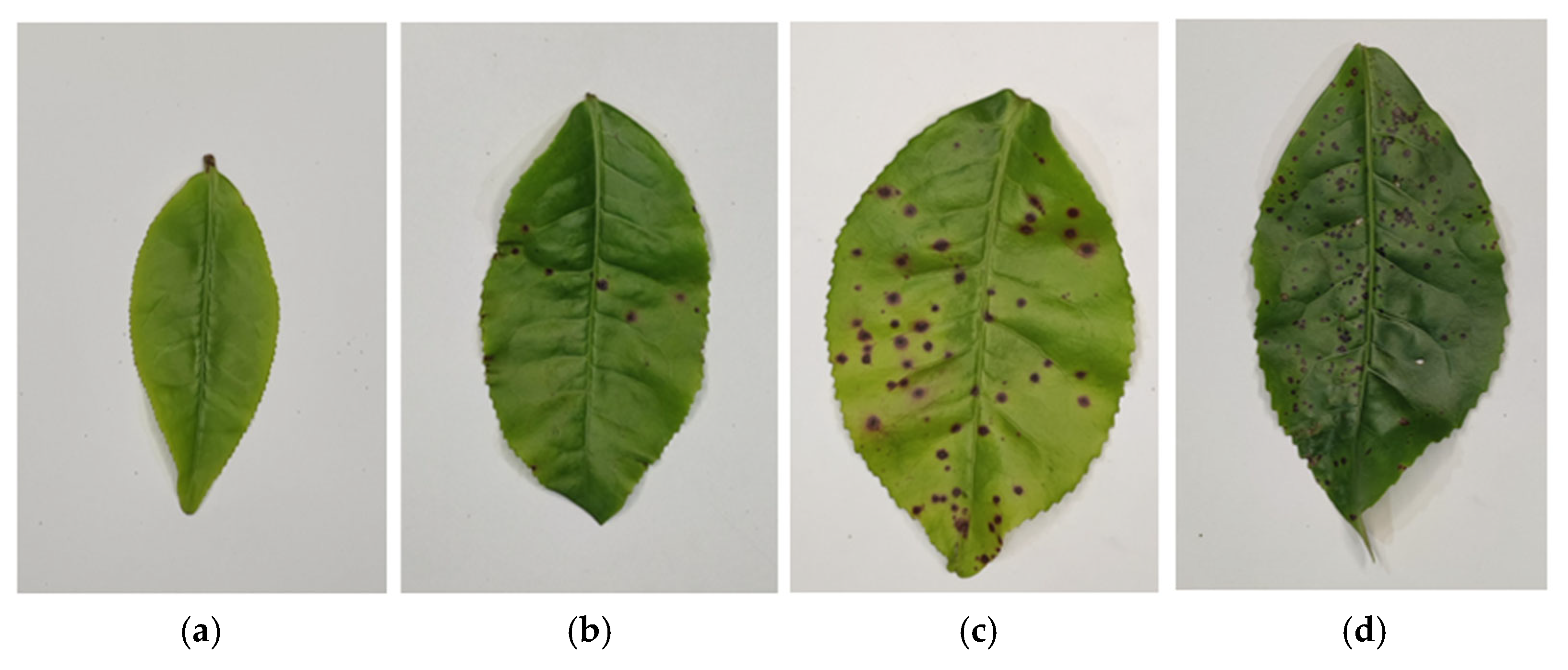
In this study, we used hyperspectral imaging technologies to develop a more accurate classification model for the grade of Tea red scab. The results of this study indicate that severity grading models for Tea red scab on RGB images exhibit inferior performance compared to those utilizing hyperspectral imagery. As described in the severity grading methodology section, developing a severity grading model from RGB images requires precise identification of tea leaf lesions. This process demands not only high-resolution imaging equipment but is also complicated by the small size of the lesions and their tendency to merge and overlap, which hinder accurate detection. These factors likely contribute to the diminished performance of RGB-based models. Figure 14 shows images of samples under four severity levels.

In contrast, the use of spectral information from hyperspectral imagery circumvents the challenges associated with small lesion size and overlapping regions. To begin, Figure 10 shows that the spectral curves of different severity classes of Tea red scab are clearly distinguishable, and when analyzed in terms of spectral properties, the spectral information on the surface of tea leaves can reflect information about its internal biochemical composition. The disease attacks the leaves, causing a lack of chlorophyll, a drop in water content, and significant changes in spectral reflectance in the visible light band [49,50]. Because the green and red light regions are sensitive to chlorophyll concentration, and the near-infrared light region is sensitive to moisture content, the overall trend in spectral reflectance was consistent throughout the four disease groups. Reflectance increased in the green light range from 490 to 560 nm, in the red light region from 680 to 760 nm, and reduced in the near-infrared light region. However, the reflectance of samples from various disease classes differed substantially in the wavelength ranges of 515–649 nm and 718–932 nm, peaking around 753 nm. This means that each sample represented by the average spectra of the leaf surface has acceptable data categorization, which is required to build an appropriate classification model.

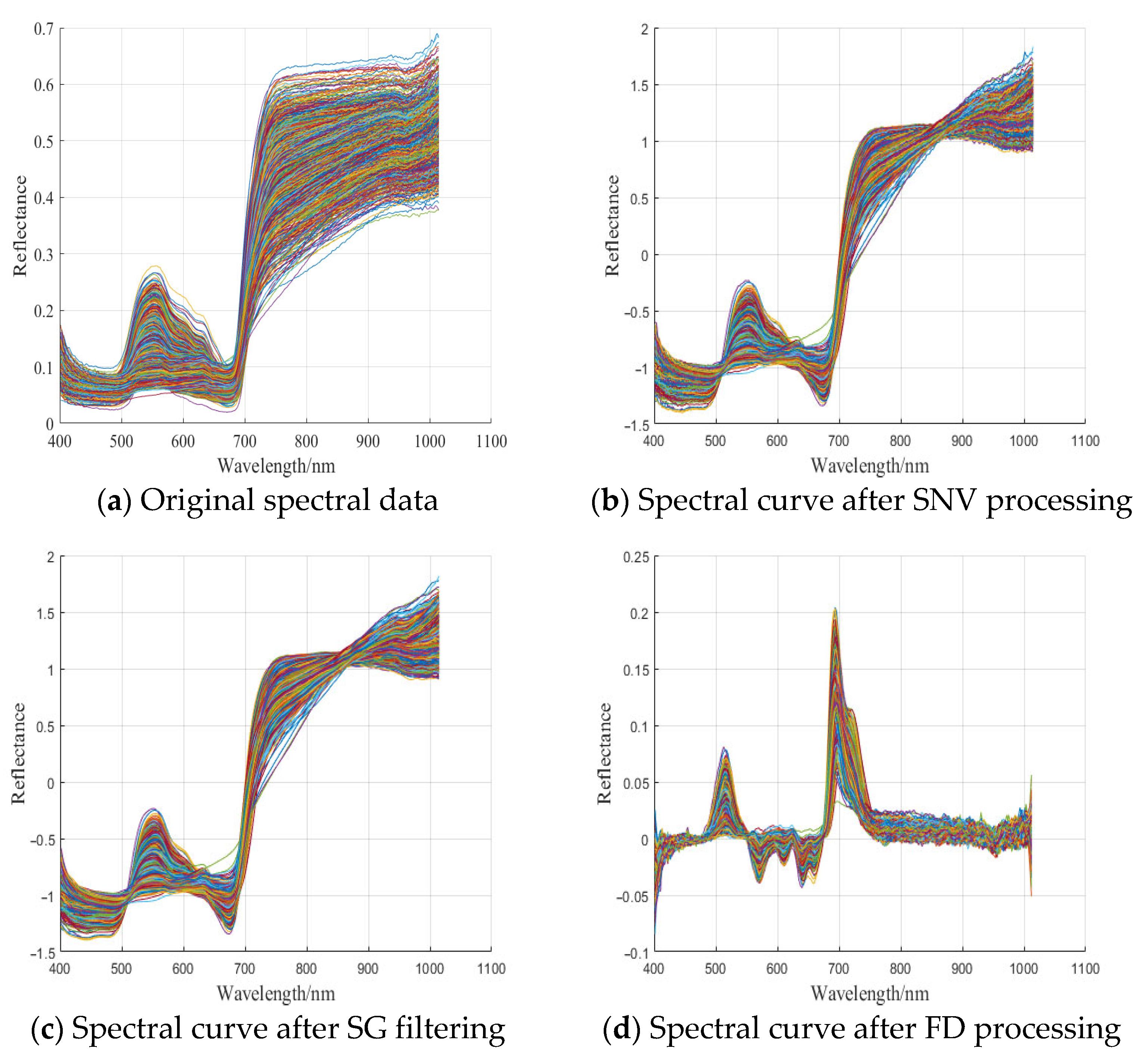
Following the selection of preprocessing methods, the results of 1D-CNN model correctness under various preprocessing approaches are compared, and it is established that SNV-SG-FD preprocessing is more efficient. The original spectra are compared to the spectral curves after each preprocessing step, and the results are given in Figure 15. SNV processing may effectively center and normalize data while also eliminating noise and signal shift in spectral data produced by scattering [51]. Figure 15a,b shows that SNV-processed spectra increase signal-to-noise ratios in the 900~1000 nm region and effectively suppress scattering noise caused by leaf surface inhomogeneity. The SG filtering uses polynomials inside a defined shifting window on the original spectra to polynomially fit the data using a least-squares method, which filters away noise while keeping the signal’s form and width constant [52]. Figure 15c shows that following SG filtering, the high-frequency oscillations of the spectral data are decreased, as is the high-frequency noise density, to make the spectral data smoother while keeping the chlorophyll absorption peak in the region near 680 nm. And the first-order derivative transform reveals the subtleties of the spectral curve by calculating the data’s first-order derivatives, which aids in the separation of overlapping peaks. The first-order derivative processes spectral data, eliminating baseline drift and improving the separation of overlapping peaks, making peaks and troughs more visible and analyzable [53]. Figure 15d depicts the spectral curves following the joint SNV-SG-FD preprocessing. After removing the scattering interference caused by SNV, the random noise is further suppressed by SG filtering, and the biochemical characteristic peaks are finally highlighted by the first-order derivative, which is more stable and has more prominent peaks and valleys than the original spectra, resulting in the model’s higher accuracy and reliability [54].

The NRBO-CNN-GRU model developed in this study produced improved results, with 92.94% accuracy, 92.54% precision, 92.42% recall, and 92.43% score, respectively, representing a considerable improvement over the single model. This could be due to the optimization algorithm working in tandem with the model, resulting in improved feature extraction. Although the 1D-CNN model can efficiently extract local spectrum characteristics, it is difficult to capture the temporal dependence of spectral sequences, resulting in a limited ability to represent disease severity categorization. Although 1D-CNN may extract local features, it is difficult to extract features from the Tea red scab severity class with high differentiation due to the similarity of the spectral properties of tea leaves, resulting in poor classification performance [55]. GRU performs better on spectral sequence data but is less sensitive to local characteristics [56]. Although basic CNN-GRU hybrid systems overcome some of these constraints, they frequently have suboptimal parameter efficiency and feature redundancy, which can diminish the classification model’s performance [57]. The NRBO algorithm, on the other hand, can overcome the restrictions of CNN-GRU by optimizing its parameters [47]. NRBO coordinates convolutional kernel size and hidden unit dimension using adaptive neighborhood radius adjustment and dynamic parameter space adjustment. Simultaneously, it can boost feature selection, reduce information overlap, and improve discriminative ability [58].

4.2. Challenges and Prospects

While this study demonstrates the utility of hyperspectral imaging for assessing Tea red scab severity, its practical deployment in tea gardens faces significant challenges. The high equipment cost, slow data transmission rates, and sensitivity to environmental factors—particularly the vulnerability of pushbroom scanning to wind interference—compromise image quality and hinder rapid field application. Nevertheless, the potential applications of hyperspectral technology extend beyond disease assessment to include monitoring tea plant nutrition and quality, thereby laying the groundwork for precise irrigation and fertilization management. Overcoming the current data acquisition bottlenecks is thus essential for realizing robust in situ monitoring and enhancing overall productivity in tea cultivation.

For the subject of this study, Tea red scab, future work should encompass not only severity assessment but also early detection. Timely identification is critical for enabling targeted pesticide application, thereby reducing tea leaf losses and improving economic benefits. Building upon the findings of this study and in response to the practical limitations of hyperspectral imaging, a low-cost spectral diagnostic system suitable for tea gardens can be developed by utilizing the key diagnostic bands identified in previous research. This transition is crucial for translating hyperspectral technology into practical applications. To address existing constraints, such a system should leverage these key wavelengths to reduce cost and complexity while also transitioning from push-broom scanning to snapshot imaging technology. This strategic shift would facilitate the design of spectral cameras specifically tailored for tea disease detection, simultaneously lowering costs and mitigating the environmental sensitivity inherent in traditional scanning systems.

Beyond hardware improvements, maintaining high model performance is essential for accurate disease monitoring. Although the model developed in this study can assess the severity of tea red rust to some extent, its training data were limited to a single variety from one region, which may constrain generalizability. Future work should expand the dataset by incorporating samples from multiple varieties and growing regions to enhance model robustness. The finalized model will be deployed on the instrument to enable rapid detection of tea red rust severity and potentially other diseases. Moreover, during practical application, it is important to continuously incorporate new data and periodically update the model to further improve adaptability and ensure long-term applicability.

5. Conclusions

This study investigated rapid severity grading models for Tea red scab using RGB and hyperspectral image datasets. Initially, models based on AlexNet, MobileNet-V2, and VGG16 architectures were developed using the RGB dataset. However, their accuracy, precision, recall, and F₁-scores all remained below 80%. The RGB-based models yielded relatively poor results. Subsequently, spectral data preprocessed using the SNV-SG-FD joint method was employed to establish classification models through four distinct approaches: CNN, GRU, CNN-GRU combination, and NRBO-CNN-GRU architecture. Each model’s performance was evaluated using four metrics alongside confusion matrix analysis. The NRBO-CNN-GRU model emerged as the top-performing framework, achieving 92.43% accuracy, 92.51% precision, 92.43% recall, and an F₁-score of 92.43%. This model was subsequently applied to assess the severity of Tea red scab, demonstrating high accuracy and robustness in practical detection tasks.

References

1. Dong, Z.F.; Li, J.; Zhao, Y. Survey of the occurency and distribution of major disease and insect pest species of tea plants in Shangluo. J. Shanxi Agric. Univ. 2018, 38, 33–37. [Google Scholar]
2. Liu, W.; Yuan, D.; Guo, G.Y.; Yang, G.Y.; Ye, N.X. Identification of anthracnose pathogen in tea plant. J. South. Agric. 2017, 48, 448–453. [Google Scholar]
3. Rong, W.Z. Investigation and research on Cercospora sp. J. Tea 1983, 1, 30–32. [Google Scholar]
4. Ponmurugan, P.; Manjukarunambika, K.; Gnanamangai, B.M. Impact of various foliar diseases on the biochemical, volatile and quality constituents of green and black teas. Australas. Plant Pathol. 2016, 45, 175–185. [Google Scholar] [CrossRef]
5. Yan, J.N.; Lu, A.X.; Kun, J.R.; Wang, B.; Miao, Y.W.; Chen, Y.J.; Ho, C.T.; Meng, Q.; Tong, H.R. Characterization of triterpenoids as possible bitter-tasting compounds in teas infected with bird’s eye spot disease. Food Res. Int. 2023, 167, 112643. [Google Scholar] [CrossRef]
6. Yan, J.N.; Miao, Y.W.; Zhou, J.Y.; Huang, R.; Dai, H.W.; Liu, M.; Lin, Y.Z.; Chen, Y.J.; Ho, C.T.; Tong, H.R.; et al. Sensory-directed isolation and identification of an intense salicin-like bitter compound in infected teas with bird’s eye spot disease. Food Res. Int. 2023, 173, 113272. [Google Scholar] [CrossRef]
7. Li, D.T.; Ren, Z.; Zhu, L.; Tang, X.M.; Fu, C.W.; Wang, Z.F.; Wang, X.Z.; Yi, K.; Hu, Y.J. Effects of soil conditioner and Bacillus subtilis fungicide on the growth and development of tobacco and diseases of tobacco. Jiangsu Agric. Sci. 2022, 50, 88–94. [Google Scholar]
8. Lou, S.; Zhang, B.R.; Zhang, D.H. Foresight from the hometown of green tea in china: Tea farmers’ adoption of pro-green control technology for tea plant pests. J. Clean. Prod. 2021, 320, 128817. [Google Scholar] [CrossRef]
9. Hu, G.S.; Wang, H.Y.; Zhang, Y.; Wan, M.Z. Detection and severity analysis of tea leaf blight based on deep learning. Comput. Electr. Eng. 2021, 90, 107023. [Google Scholar] [CrossRef]
10. Trippa, D.; Scalenghe, R.; Basso, F.M.; Panno, S.; Davino, S.; Morone, C.; Giovino, A.; Oufensou, S.; Luchi, N.; Yousefi, S.; et al. Next-generation methods for early disease detection in crops. Pest. Manag. Sci. 2023, 80, 245–261. [Google Scholar] [CrossRef]
11. Donahue, C.P.; Menounos, B.; Viner, N.; Skiles, S.M.; Beffort, S.; Denouden, T.; Arriola, S.G.; White, R.; Heathfield, D. Bridging the gap between airborne and spaceborne imaging spectroscopy for mountain glacier surface property retrievals. Remote Sens. Environ. 2023, 299, 113849. [Google Scholar] [CrossRef]
12. Chen, J.; Liu, Q.; Gao, L. Visual tea leaf disease recognition using a convolutional neural network model. Symmetry 2019, 11, 343. [Google Scholar] [CrossRef]
13. Wu, P.; Cai, M.D.; Yi, X.M.; Wang, G.Y.; Mo, L.F.; Chola, M.; Kapapa, C. Sweetgum Leaf Spot Image Segmentation and Grading Detection Based on an Improved DeeplabV3+ Network. Forests 2023, 14, 1547. [Google Scholar] [CrossRef]
14. Zhang, T.; Xuan, C.Z.; Ma, Y.H.; Tang, Z.H.; Gao, X.Y. An efficient and precise dynamic neighbor graph network for crop mapping using unmanned aerial vehicle hyperspectral imagery. Comput. Electron. Agric. 2025, 230, 109838. [Google Scholar] [CrossRef]
15. Hu, Y.T.; Ma, B.X.; Wang, H.T.; Li, Y.J.; Zhang, Y.J.; Yu, G.W. Non-Destructive Detection of Different Pesticide Residues on the Surface of Hami Melon Classification Based on tHBA-ELM Algorithm and SWIR Hyperspectral Imaging. Foods 2023, 12, 1173. [Google Scholar] [CrossRef]
16. Tang, T.; Luo, Q.; Yang, L.; Gao, C.L.; Ling, C.J.; Wu, W.B. Research review on quality detection of fresh tea leaves based on spectral technology. Foods 2023, 13, 25. [Google Scholar] [CrossRef] [PubMed]
17. Zhao, X.H.; Zhang, J.C.; Huang, Y.B.; Tian, Y.Y.; Yuan, L. Detection and discrimination of disease and insect stress of tea plants using hyperspectral imaging combined with wavelet analysis. Comput. Electron. Agric. 2022, 193, 106717. [Google Scholar] [CrossRef]
18. Zou, X.G.; Zhang, J.; Huang, S.Y.; Wang, J.P.; Yao, H.Y.; Song, Y.Y. Recognition of tea diseases under natural background based on particle swarm optimization algorithm optimized support vector machine. In Proceedings of the 2020 IEEE 18th International Conference on Industrial Informatics (INDIN), Warwick, UK, 20–23 July 2020; Volume 1, pp. 547–552. [Google Scholar]
19. Lin, Y.H.; Lin, X.R.; Chen, S.F. Application of hyperspectral imaging for identification of types and levels of pest damage on tea leaves. In Proceedings of the 2023 American Society of Agricultural and Biological Engineers Annual International Meeting, Omaha, NE, USA, 9–12 July 2023. [Google Scholar]
20. Zhang, J.; Zhao, Z.X.; Zhao, Y.R.; Bu, H.C.; Wu, X.Y. Oilseed Rape Sclerotinia in Hyperspectral Images Segmentation Method Based on Bi-GRU and Spatial-Spectral Information Fusion. Smart Agric. 2024, 6, 40–48. [Google Scholar]
21. Saviolo, A.; Bonotto, M.; Evangelista, D.; Imperoli, M.; Lazzaro, J.; Menegatti, E.; Pretto, A. Learning to segment human body parts with synthetically trained deep convolutional networks. In Proceedings of the International Conference on Intelligent Autonomous Systems, Wuhan, China, 14–16 May 2021; Springer International Publishing: Cham, Switzerland, 2021; Volume 412, pp. 696–712. [Google Scholar]
22. Li, J.Q.; Zhao, X.Y.; Xu, H.N.; Zhang, L.M.; Xie, B.Y.; Yan, J.; Zhang, L.C.; Fan, D.C.; Li, L. An Interpretable High-Accuracy Method for Rice Disease Detection Based on Multisource Data and Transfer Learning. Plants 2023, 12, 3273. [Google Scholar] [CrossRef]
23. Yang, Z.; Guo, Y.G.; Lu, X.B. Classification Method of UAV Remote Sensing ImageBased on Improved AlexNet Network. J. Hunan Univ. Sci. Technol. Nat. Sci. Ed. 2023, 38, 59–69. [Google Scholar]
24. Cui, L.H.; Yan, L.J.; Zhao, X.H.; Yuan, L.; Jin, J.; Zhang, J.C. Detection and Discrimination of Tea Plant Stresses Based on Hyperspectral Imaging Technique at a Canopy Level. Phyton 2021, 90, 621–634. [Google Scholar] [CrossRef]
25. Zhu, L.; Li, Z.B.; Li, C.; Wu, J.; Yue, J. High performance vegetable classification from images based on AlexNet deep learning model. Int. J. Agric. Biol. Eng. 2018, 11, 217–223. [Google Scholar] [CrossRef]
26. Krizhevsky, A.; Sutskever, I.; Hinton, E.G. ImageNet classification with deep convolutional neural networks. Commun. ACM 2017, 60, 84–90. [Google Scholar] [CrossRef]
27. Jiang, Z.P.; Liu, Y.Y.; Shao, Z.E.; Huang, K.W. An improved VGG16 model for pneumonia image classification. Appl. Sci. 2021, 11, 11185. [Google Scholar] [CrossRef]
28. Dai, A.X.; Xiao, Y.C.; Li, D.C.; Xue, J.Y. Status Recognition of Magnetic Fluid Seal Based on High-Order Cumulant Image and VGG16. Front. Mater. 2022, 9, 929795. [Google Scholar] [CrossRef]
29. Chen, L.C.; Sheu, R.K.; Peng, W.Y.; Wu, H.J.; Tseng, C.H. Video-based parking occupancy detection for smart control system. Appl. Sci. 2020, 10, 1079. [Google Scholar] [CrossRef]
30. Yun, J.T.; Jiang, D.; Liu, Y.; Sun, Y.; Tao, B.; Kong, J.Y.; Tian, J.R.; Tong, X.L.; Xu, M.M.; Fang, Z.F. Real-Time Target Detection Method Based on Lightweight Convolutional Neural Network. Front. Bioeng. Biotechnol. 2022, 10, 861286. [Google Scholar] [CrossRef] [PubMed]
31. He, Z.T.; Ding, L.Y.; Ji, J.T.; Jin, X.; Feng, Z.H.; Hao, M.C. Design and experiment of variable-spray system based on deep learning. Appl. Sci. 2024, 14, 3330. [Google Scholar] [CrossRef]
32. Han, Y.H.; Wang, B.; Yang, J.Y.; Yin, F.; He, L.S. Research on Hyperspectral Inversion of Soil Organic Carbon in Agricultural Fields of the Southern Shaanxi Mountain Area. Remote Sens. 2025, 17, 600. [Google Scholar] [CrossRef]
33. Tang, S.Q.; Zhong, N.; Zhou, Y.H.; Chen, S.B.; Dong, Z.B.; Qi, L.; Feng, X. Synergistic spectral-spatial fusion in hyperspectral Imaging: Dual attention-based rice seed varieties identification. Food Control 2025, 176, 111411. [Google Scholar] [CrossRef]
34. Qin, Y.W.; Zhao, Q.; Zhou, D.; Shi, Y.B.; Shou, H.Y.; Li, M.X.; Zhang, W.; Jiang, C.X. Application of flash GC e-nose and FT-NIR combined with deep learning algorithm in preventing age fraud and quality evaluation of pericarpium citri reticulatae. Food Chem. X 2024, 21, 101220. [Google Scholar] [CrossRef]
35. Li, P.; Zhang, X.X.; Li, S.K.; Du, G.R.; Jiang, L.W.; Liu, X.; Ding, S.H.; Shan, Y. A rapid and nondestructive approach for the classification of different-age citri reticulatae pericarpium using portable near infrared spectroscopy. Sensors 2020, 20, 1586. [Google Scholar] [CrossRef]
36. Cheng, T.; Chen, G.; Wang, Z.C.; Hu, R.J.; She, B.; Pan, Z.G.; Zhou, X.G.; Zhang, G.; Zhang, D.Y. Hyperspectral and imagery integrated analysis for vegetable seed vigor detection. Infrared Phys. Technol. 2023, 131, 104605. [Google Scholar] [CrossRef]
37. Tang, Y.Z.; Li, F.; Hu, Y.C.; Yu, K. NTRI: A novel spectral index for developing a precise nitrogen diagnosis model across pre- and post-anthesis stages of maize plants. Field Crop Res. 2025, 325, 109829. [Google Scholar] [CrossRef]
38. Zhou, X.K.; Yu, J.B. Gearbox Fault Diagnosis Based on One-dimension Residual Convolutional Auto-encoder. J. Mech. Eng. Chin. Ed. 2020, 56, 96–108. [Google Scholar]
39. Huang, M.; Xie, X.G.; Sun, W.W.; Li, Y.M. Tool wear prediction model using multi-channel 1d convolutional neural network and temporal convolutional network. Lubricants 2024, 12, 36. [Google Scholar] [CrossRef]
40. Xie, C.; Xue, B.; Yang, M.Y.; Zhang, M.J.; Xu, Z.G.; Wang, J.Y.; Chen, S.L.; Liu, Y. Evolutionary neural architecture search for automatically designing CNN-GRU-Attention neural networks for turntable servo systems. Expert. Syst. Appl. 2025, 283, 127765. [Google Scholar] [CrossRef]
41. Arathy, N.G.R.; Adarsh, S. Innovative knowledge-based system for streamflow hindcasting: A comparative assessment of Gaussian Process-Integrated Neural Network with LSTM and GRU models. Environ. Model. Softw. 2025, 188, 106433. [Google Scholar]
42. Hu, H.; Lu, H.; Shi, R.J.; Fan, X.C.; Deng, Z.H. A novel fault diagnosis method for key transmission sections based on Nadam-optimized GRU neural network. Electr. Power Syst. Res. 2024, 233, 110522. [Google Scholar] [CrossRef]
43. Zhou, H.T.; Chen, W.H.; Liu, J.; Cheng, L.S.; Xia, M. Trustworthy and intelligent fault diagnosis with effective denoising and evidential stacked GRU neural network. J. Intell. Manuf. 2023, 35, 3523–3542. [Google Scholar] [CrossRef]
44. Sowmya, R.; Manoharan, P.; Pradeep, J. Newton-Raphson-based optimizer: A new population-based metaheuristic algorithm for continuous optimization problems. Eng. Appl. Artif. Intell. 2024, 128, 107532. [Google Scholar] [CrossRef]
45. Lindstrom, M.J.; Bates, D.M. Newton—Raphson and EM Algorithms for Linear Mixed-Effects Models for Repeated-Measures Data. J. Am. Stat. Assoc. 1988, 83, 1014–1022. [Google Scholar]
46. Ahmadianfar, I.; Bozorg-Haddad, O.; Chu, X. Gradient-based optimizer: A new metaheuristic optimization algorithm. Inf. Sci. 2020, 540, 131–159. [Google Scholar] [CrossRef]
47. Li, Y.; Liu, H.; Lu, F. Research on prediction of ash content in flotation-recovered clean coal based on nrbo-cnn-lstm. Minerals 2024, 14, 894. [Google Scholar] [CrossRef]
48. Guo, X.Y.; Hu, Q.H.; Liu, C.P.; Yang, J.W. Food image recognition based on transfer learning and batch normalization. Comput. Appl. Softw. 2021, 38, 124–133. [Google Scholar]
49. Junges, A.H.; Marcus, A.K.A.; Thor, V.M.F.; Jorge, R.D. Leaf hyperspectral reflectance as a potential tool to detect diseases associated with vineyard decline. Trop. Plant Pathol. 2020, 45, 522–533. [Google Scholar] [CrossRef]
50. Lu, B.; Dao, P.D.; Liu, J.; He, Y.; Shang, J. Recent Advances of Hyperspectral Imaging Technology and Applications in Agriculture. Remote Sens. 2020, 12, 2659. [Google Scholar] [CrossRef]
51. Ma, H.Y.S.; Pan, N.; Lin, Z.Y.; Chen, X.T.; Wu, J.N.; Zhang, F.; Liu, Z.Y. Research Progress on the Vibrational Spectroscopy Technology in the Quality Detection of Fish Oil. Spectrosc. Spectr. Anal. 2025, 45, 301–311. [Google Scholar]
52. Bouslihim, Y.; Bouasria, A. Potential of EnMAP Hyperspectral Imagery for Regional-Scale Soil Organic Matter Mapping. Remote Sens. 2025, 17, 1600. [Google Scholar] [CrossRef]
53. Qi, H.M.; Chen, A.; Yang, X.C.; Xing, X.Y. Estimation of crude protein content in natural pasture grass using unmanned aerial vehicle hyperspectral data. Comput. Electron. Agric. 2025, 229, 109714. [Google Scholar] [CrossRef]
54. He, J.C.; He, J.; Liu, G.; Li, W.L.; Li, Z.; Li, Z. Inversion analysis of soil nitrogen content using hyperspectral images with different preprocessing methods. Ecol. Inf. 2023, 78, 102381. [Google Scholar]
55. Li, H.Z.; Xu, S.H.; Teng, J.H.; Jiang, X.H.; Zhang, H.; Qin, Y.Z.; He, Y.S.; Fan, L. Deep learning assisted ATR-FTIR and Raman spectroscopy fusion technology for microplastic identification. Microchem. J. 2025, 212, 113224. [Google Scholar] [CrossRef]
56. Li, X.L.; Yu, J.; Zhang, H.Y.; Dong, L.; Zhang, Z.D.; Li, K.; Yu, Y.Q.; Li, Q. Improved Attention Mechanism MobileNetV2 Network for SERS Classification of Water Pollution. Laser Optoelectron. Prog. 2025, 62, 073004. [Google Scholar]
57. Muzakka, K.; Sören, M.; Stefan, K.; Jan, E.; Alina, B.; Helene, H.; Sebastian, S.; Martin, F. Analysis of Rutherford backscattering spectra with CNN-GRU mixture density network. Sci. Rep. 2024, 14, 16983. [Google Scholar] [CrossRef] [PubMed]
58. Jiang, X.; Cao, X.; Liu, Q.; Wang, F.; Fan, S.; Yan, L.; Wei, Y.; Chen, Y.; Yang, G.; Xu, B.; et al. Prediction of multi-task physicochemical indices based on hyperspectral imaging and analysis of the relationship between physicochemical composition and sensory quality of tea. Food Res. Int. 2025, 19, 116455. [Google Scholar] [CrossRef] [PubMed]
Figure 1. Overall flowchart.
Agriculture 15 02372 g001
Figure 2. Overview of the study sampling area.
Agriculture 15 02372 g002
Figure 3. Hyperspectral acquisition system.
Agriculture 15 02372 g003
Figure 4. Data augmentation schematic diagram. (a) Original image; (b) Sharpened image.
Agriculture 15 02372 g004
Figure 5. AlexNet architecture diagram.
Agriculture 15 02372 g005
Figure 6. Architecture diagram.
Agriculture 15 02372 g006
Figure 7. Depthwise separable convolution.
Agriculture 15 02372 g007
Figure 8. Inverse residual structure.
Agriculture 15 02372 g008
Figure 9. GRU model network structure diagram.
Agriculture 15 02372 g009
Figure 10. CNN-GRU composite network structure.
Agriculture 15 02372 g010
Figure 11. Schematic diagram of sample spectral reflectance extraction. (a) Select ROI to extract reflectivity; (b) Average spectral reflectance of sample leaves.
Agriculture 15 02372 g011
Figure 12. Model performance for different sample categories. (a) Different modelling results for healthy samples; (b) Different modelling results for samples in the mild disease class; (c) Different modelling results for samples with moderate disease grades; (d) Different modelling results for samples in the severe disease class.
Agriculture 15 02372 g012aAgriculture 15 02372 g012b
Figure 13. Model performance for different sample categories. (a) RAW + CNN; (b) Processing + CNN; (c) RAW + GRU; (d) Processing + GRU; (e) RAW + CNN-GRU; (f) Processing + CNN-GRU; (g) RAW + GRU; (h) Processing + NRBO-CNN-GRU.
Agriculture 15 02372 g013aAgriculture 15 02372 g013b
Figure 14. Sample images of tea leaf round red spot disease at different severity levels. (a) Health; (b) Minor; (c) Medium; (d) Severe.
Agriculture 15 02372 g014
Figure 15. Schematic diagram of spectral preprocessing. (a) Raw spectral data; (b) Spectral curve after SNV treatment; (c) SG filtered spectral profile; (d) Spectral curve after FD treatment.
Agriculture 15 02372 g015