Article

Fusion of LSTM-Based Vertical-Gradient Prediction and 3D Kriging for Greenhouse Temperature Field Reconstruction

1
College of Software, Shanxi Agricultural University, Jinzhong 030801, China
2
College of Agricultural Engineering, Shanxi Agricultural University, Jinzhong 030801, China
3
Shanxi Academy of Agricultural Sciences, Pomology Institute, Jinzhong 030815, China
4
College of Horticultural, Shanxi Agricultural University, Jinzhong 030801, China
*
Author to whom correspondence should be addressed.
Agriculture 2025, 15(21), 2222; https://doi.org/10.3390/agriculture15212222 (registering DOI)
Submission received: 17 September 2025 / Revised: 10 October 2025 / Accepted: 23 October 2025 / Published: 24 October 2025
(This article belongs to the Section Artificial Intelligence and Digital Agriculture)

Abstract

This paper presents a proposed LSTM-based vertical-gradient prediction combined with three-dimensional kriging that enables reconstruction of greenhouse 3D temperature fields under sparse-sensor deployments while capturing temporal dynamics and spatial correlations. In northern China, winter solar greenhouses rely on standardized structures and passive climate-control strategies, which often lead to non-uniform thermal conditions that complicate precise regulation. To address this challenge, 24 sensors were deployed, and their time-series data were used to train a long short-term memory (LSTM) model for vertical temperature-gradient prediction. The predicted values at multiple heights were fused with in situ observations, and three-dimensional ordinary kriging (3D-OK) was applied to reconstruct the spatiotemporal temperature field. Compared with conventional 2D monitoring and computationally intensive CFD, the proposed approach balances accuracy, efficiency, and deployability. LSTM–Kriging validation showed Trend + Residual Kriging had the lowest RMSE (0.45558 °C) and bias (−0.03148 °C) (p < 0.01), outperforming Trend-only RMSE (3.59 °C) and Kriging-only RMSE (0.48 °C); the 3D model effectively distinguished sunny and rainy dynamics. This cost-effective framework balances accuracy, efficiency, and deployability, overcoming limitations of 2D monitoring and CFD. It provides critical support for adaptive greenhouse climate regulation and digital-twin development, directly advancing precision management and yield stability in CEA.

1. Introduction

Controlled-environment agriculture (CEA) plays a pivotal role in global food production and sustainability. With population growth and continuing loss of arable land, achieving high and stable yields in limited space has become a central challenge for agricultural science and engineering. Greenhouses, as a core CEA technology, regulate the internal microclimate to provide stable growing conditions for crops [1]. In northern China, solar greenhouses are widely used; their passive temperature-control features—such as heat storage in earthen walls and natural ventilation—offer energy-saving benefits. However, structural heterogeneity and localized microclimates often produce pronounced spatial nonuniformity and vertical temperature gradients, which reduce photosynthetic efficiency, complicate precise environmental control, and can lower yields.
To address these challenges, recent studies have explored advanced control strategies that integrate Internet of Things (IoT) monitoring with machine learning for intelligent greenhouse climate management [2], as well as novel modeling approaches such as Bayesian Neural ODEs for crop-specific temperature prediction [3]. Despite these advances, existing work remains limited in its ability to capture three-dimensional (3D) spatial temperature gradients under sparse-sensor deployments, motivating the development of the method proposed in this study.
Temperature is a primary determinant of crop physiological processes; it directly affects photosynthesis, transpiration, nutrient metabolism, and pest and disease dynamics [4,5]. Spatial temperature nonuniformity within a greenhouse leads to heterogeneous crop growth, increases energy consumption, and lowers yields. Therefore, rigorous characterization of the internal temperature field—especially its three-dimensional (3D) variability—is essential. Such knowledge enables targeted environmental control, improves energy efficiency, and supports intelligent greenhouse management [6].
In recent years, researchers worldwide have extensively studied greenhouse temperature modeling and spatial temperature distributions; overall, work falls into three methodological categories: sensor-based monitoring, numerical simulation (CFD), and statistical/machine-learning modeling. Sensor-based approaches deploy temperature sensors at multiple locations to obtain real-time, in situ measurements; these point measurements are high-fidelity but require dense networks for high spatial resolution, which increases capital and maintenance costs, and sparse sensors alone cannot capture the continuous 3D temperature structure [7,8,9]. To overcome these gaps, many studies use CFD to reconstruct airflow and temperature distributions and to evaluate ventilation, shading, and canopy effects—an approach widely applied for analyzing greenhouse thermal environments [10]. While CFD offers high-fidelity representations of airflow and heat transfer [11], its results are sensitive to mesh resolution, turbulence models, and boundary conditions; moreover, it requires substantial computational resources and measurement-based calibration [12,13,14], and its high computational demand further limits real-time applicability [10,11]. Complementarily, statistical and machine-learning methods (time-series forecasting, spatial interpolation/regression and data-driven surrogates) have been used to infer and forecast temperatures with lower computational cost and for real-time applications, though their generalizability depends on training-data representativeness and feature selection [7,14]. Consequently, recent work increasingly adopts hybrid strategies that combine sensors, CFD and data-driven models to balance measurement fidelity, spatial coherence and deployment cost [7,12].
A third research direction involves statistical and data-driven methods, such as kriging interpolation and deep learning (DL), which efficiently learn nonlinear relationships from limited sensor data. Recent works have sought to integrate DL with CFD or geostatistical interpolation to overcome these limitations. For example, recent studies have combined deep learning with CFD and geostatistical interpolation to improve dynamic temperature prediction and spatial reconstruction; however, most of these efforts focus on 2D fields or assume relatively dense sensing and thus do not achieve full 3D reconstruction under sparse-sensor deployments [10,12,14,15].
Building on these developments, deep learning models—particularly long short-term memory (LSTM) networks—have shown strong performance in capturing nonlinear and temporal dependencies in greenhouse environments [16,17,18]. While Transformer-based architectures (e.g., Temporal Fusion Transformer, TFT) demonstrate superior scalability on large datasets, they remain computationally expensive and less suited to small-scale, sensor-limited applications [19,20]. Despite this progress, few studies have coupled DL-based temporal prediction with spatial interpolation to reconstruct full 3D temperature fields under sparse sensing—highlighting the need for a lightweight, integrated framework.
A review of existing research reveals four persistent gaps in greenhouse temperature modeling and spatial distribution studies. To further clarify the methodological landscape, Table 1 summarizes representative studies, their methodological categories, and associated advantages and limitations.
To address these gaps, we propose and validate a combined approach that couples LSTM-based vertical-gradient prediction with three-dimensional (3D) ordinary kriging. Under sparse-sensor deployments, the method jointly captures temporal dynamics and spatial correlations to reconstruct a 3D greenhouse temperature field spanning a full diurnal cycle and the 0–3 m vertical domain, and we evaluate it under two typical weather regimes—sunny and rainy days. Methodologically, this work advances greenhouse environmental modeling by integrating temporal deep learning with spatial statistics to capture vertical gradients and spatial correlations from limited sensors. Practically, it provides a low-cost, accurate solution for intelligent greenhouse control and digital-twin construction: reconstructing the 3D temperature field enables more precise decisions on ventilation, shading, and heating, thereby improving energy efficiency and crop performance. The approach is extensible to other controlled-environment facilities such as plastic greenhouses and plant factories [23].

2. Data Acquisition and Feature Engineering

2.1. Overview of the Experimental Greenhouse

The experiment was conducted in a solar greenhouse at the Fruit Tree Research Institute, Shanxi Agricultural University (37.34° N, 112.49° E). The site has a temperate continental climate, with a long-term mean air temperature of 10.4 °C, an annual sunshine duration of 2527.5 h, and annual precipitation of approximately 397.1 mm. The greenhouse was oriented east–west and measured 60 m × 10 m × 5 m (length × width × height) and featured earthen walls. Strawberry (cv. “Zhangji”) was chosen as the model crop because it is a representative fruit crop in solar greenhouses, characterized by a dense canopy and strong sensitivity to temperature fluctuations. Its layered canopy structure and low growth height accentuate vertical temperature gradients, making it ideal for studying three-dimensional thermal heterogeneity.
The study employed an RS-QXZ-M IoT meteorological data logger (Shandong JianDa RenKe, Jinan, China), powered at 24 V DC. Data were transmitted in real time over a 4G cellular network to a cloud database, and system clocks were synchronized to a national time server via the Network Time Protocol (NTP).
Indoor air temperature was measured using 24 polyethylene (PE) temperature probes (accuracy ± 0.5 °C; Shandong JianDa RenKe, Jinan, China). The sensors are waterproof and dustproof, suitable for high-humidity greenhouse environments. Before deployment, all probes were factory-calibrated and cross-validated against a reference mercury thermometer (±0.1 °C) under stable laboratory conditions to minimize systematic bias. Although the nominal precision of ±0.5 °C is moderate, such accuracy is widely adopted in greenhouse studies due to the balance between cost and measurement stability. Moreover, since the study focuses on relative spatial variations rather than absolute temperature values, this precision is adequate for reliable three-dimensional kriging interpolation. Sampling was synchronized across all sensors at 30 min intervals, and data were collected continuously from 1 May to 1 June 2025. To facilitate temporal analysis, the full 31-day dataset (1488 samples per sensor) was divided into eight consecutive subsets, each covering approximately 3–4 days (≈186 samples per subset). This segmentation captured gradual thermal transitions during late spring and early summer and provided statistically robust samples for model training and validation.
Six equally spaced north–south vertical sampling planes were located 5, 15, 25, 35, 45, and 55 m from the west wall. At each plane, three temperature sensors were installed at 1.5 m above floor level (strawberries are grown on 1 m-high racks; 1.5 m is above the canopy), yielding 18 points (s1–s18). An additional vertical profiling plane at 45 m from the west wall included three sensors at ground level (0 m) and three near the arch apex (3 m), for six points (h1–h6). This vertical arrangement was designed to capture temperature gradients from the ground to the canopy and roof, thereby overcoming the 2D limitations identified in the introduction. Figure 1 illustrates the layout of temperature and humidity sensors in the greenhouse. To ensure data quality, all sensors were bench-calibrated prior to deployment and field-checked monthly.
Sensor deployment was designed to ensure balanced spatial coverage and representativeness. Table 2 summarizes the horizontal layout: 18 sampling points distributed along the main (east–west) axis at 5, 15, 25, 35, 45, and 55 m from the west wall. Points are arranged on three transverse (north–south) lines at y = 3.0, 6.5, and 9.0 m across the 10 m width. All horizontal sensors were installed at 1.5 m (canopy height) to capture canopy-level temperature. This configuration resolves temperature variation in both the longitudinal (east–west) and transverse (north–south) directions throughout the greenhouse.
Additionally, a vertical profiling array was installed in the central section of the greenhouse to capture temperature distributions at multiple heights (Table 3). Six vertical sampling points were configured: three at z = 3.0 m (elevated) and three at z = 0.0 m (near ground). Horizontally, the points were located at y = 3.0, 6.5, and 9.0 m.

2.2. Data Preprocessing and Feature Variable Construction

2.2.1. Missing Value Handling and Outlier Correction

Raw sensor data may include missing values and outliers due to communication dropouts, sensor faults, or external interference. First, exploratory statistics were computed for all variables, and outliers were removed using the “3σ” rule—mean ± 3 standard deviations (SDs) [24]. This approach was selected because the greenhouse temperature series closely followed a Gaussian-like distribution under continuous measurement, and the 3σ criterion effectively isolates sporadic sensor spikes while retaining natural temperature extremes. The validity of this rule was confirmed by comparison with an interquartile range (IQR) filter, which yielded nearly identical retained-sample ratios (<1% deviation).
Second, short-term (<1 h) gaps were imputed by linear interpolation [25]. For continuous gaps longer than 1 h, values were imputed with the mean from a comparable time window (e.g., the same time of day on the previous day). This strategy leverages the strong diurnal periodicity of greenhouse temperature patterns. To prevent excessive smoothing of thermal dynamics, mean-based imputation was restricted to gaps ≤ 3 h, and variance rescaling was applied afterward to preserve natural fluctuations.
Additionally, to avoid artifacts from inconsistent sampling rates during model training, all data were resampled to a uniform 30 min interval and time-aligned using timestamps.

2.2.2. Feature Selection and Lagged Variable Design

We analyzed n = 1488 observations collected at 30 min intervals from 1 to 31 May 2025, using Pearson’s correlation coefficient (Equation (1)) [26]. For each candidate feature, we computed its correlation with temperatures at multiple in-greenhouse locations and the associated p-value for testing the null hypothesis of zero linear correlation (Equations (2) and (3)).
R = i = 1 n ( X i   X ) ( Y i Y ) i = 1 n ( X i   X ) 2 i = 1 n ( Y i Y ) 2
t = R n   2 1     r 2
p = 2   ×   P ( T n 2   >   t )
In Equation (1), X i and Y i represent the two variable values of the i -th sample point, n denotes the sample size, X and Y denote the respective means of X and Y , R is the Pearson correlation coefficient, p is the probability of observing the current or more extreme R values under the null hypothesis (no correlation), and T n 2 is a t-distributed random variable with n 2 degrees of freedom. p < 0.001 indicates highly significant correlation, 0.001 ≤ p < 0.01 indicates moderately significant correlation, 0.01≤ p < 0.05 indicates significant correlation, and p ≥ 0.05 indicates no significant correlation. The calculations for temperature sensors s10, s11, and s12 with h1, h2, h3, h4, h5, and h6 are shown in Table 4.

2.2.3. Data Normalization

To accelerate convergence and reduce the effects of heterogeneous scales, all continuous predictors (e.g., temperature, humidity, and radiation) were scaled to the [0, 1] range via min–max normalization. The scaling is defined in Equation (4) [27].
r = d     d min d max     d min
In Equation (4), d denotes the raw value; d min and d max are the minimum and maximum of the raw data series, respectively; and r is the normalized value. This normalization method was adopted because the environmental variables used as predictors (temperature, humidity, radiation) have bounded and physically meaningful ranges, which align well with the assumptions of min–max scaling. In addition, this scaling ensures numerical stability and efficient gradient flow in neural networks employing sigmoid or tanh activation functions. Preliminary tests showed that z-score normalization produced similar accuracy (<1.5% RMSE difference), confirming that the chosen method does not introduce bias.

3. Model Construction and Forecasting Methods

3.1. Construction of a Vertical-Gradient Model Based on Deep Learning

To benchmark different time-series models for greenhouse temperature prediction, three representative deep learning architectures were considered: LSTM, GRU, and Temporal Fusion Transformer (TFT).All models were implemented in Python 3.10 (Python Software Foundation, Wilmington, DE, USA) using the PyTorch 2.0 framework (Meta Platforms, Inc., Menlo Park, CA, USA).
Transformers were originally introduced for sequence modeling in natural language processing but have since been adapted for time-series forecasting to address the limitations of recurrent networks in modeling long-range dependencies and parallel computation. The TFT extends the standard Transformer with static covariate encoding and variable selection mechanisms, offering strong interpretability for heterogeneous inputs [28]. However, its high parameterization and data demands increase the risk of overfitting in medium-sized datasets.
The GRU is a simplified recurrent architecture with fewer parameters than the LSTM, enabling faster training but providing less flexibility for capturing long-term dependencies [29].
The LSTM remains a widely validated architecture for multivariate time-series forecasting due to its gated memory mechanism that effectively mitigates gradient vanishing [17]. In this study, preliminary experiments showed that GRU and TFT achieved similar accuracy (<2% RMSE difference) but required longer convergence times and exhibited greater instability during training. Therefore, the LSTM was selected as the optimal compromise between modeling capacity, stability, and computational efficiency.
Model workflow: As illustrated in Figure 2, the LSTM model takes a 12-step input sequence with three features and outputs six temperature predictions corresponding to different greenhouse positions. Each input–output pair was generated using a sliding window, with a chronological train/validation/test split (8:1:1). Continuous predictors were scaled to [0, 1] using min–max normalization (fit on the training set). The network consists of two stacked LSTM layers (64 hidden units each) followed by a fully connected layer mapping the 64-dimensional latent state to six outputs. Predictions were subsequently inverse-transformed to recover physical temperature values.

3.2. Implementation Details and Model Evaluation

We trained the model with Adam (initial learning rate 1 × 10⁻³), batch size 32, for 50 epochs. To improve stability and mitigate overfitting, we applied dropout and early stopping. The Gaussian Error Linear Unit (GELU) was used as the activation function. Training and validation were conducted in a Python 3.10 environment.
We evaluated model performance using four standard metrics: MAE (mean absolute error), MSE (mean squared error), RMSE (root mean squared error), and R2 (coefficient of determination). MAE quantifies the average absolute deviation between predictions and observations; MSE is the mean of squared errors and penalizes large deviations; RMSE is the square root of MSE and is expressed in the same units as the target. R2 measures the proportion of variance explained by the model; values closer to 1 indicate a better fit. Formal definitions are provided in Equations (5)–(8).
MAE = 1 n i = 1 n y i y ^ i
MSE = 1 n i = 1 n ( y i     y ^ i ) 2
RMSE = 1 n i = 1 n ( y i y ^ i ) 2
R 2 = 1   i = 1 n ( y i     y ^ i ) 2 i = 1 n ( y i     y ) 2
In Equations (5)–(8), n denotes the sample size; y i is the i-th observed (ground-truth) value; y ^ i is the i-th predicted value; and y is the mean of the observed values.

3.3. Three-Dimensional Temperature Modeling in Greenhouse Spaces

To reconstruct an all-weather, high-resolution three-dimensional (3D) temperature field in greenhouses with sparse sensors and airflow strongly constrained by enclosure geometry and heat-exchange conditions, we employed a hybrid approach that couples LSTM-based vertical-gradient prediction with 3D ordinary kriging (3D-OK). This approach maximizes the utility of scarce vertical observations and leverages geostatistics to model the field’s spatial correlation (via a variogram), enabling temperature predictions at arbitrary locations across the greenhouse grid.

3.3.1. Three-Dimensional Ordinary Kriging Spatial Interpolation Method

After collecting temperature observations at three vertical levels, we applied three-dimensional ordinary kriging (3D-OK) to interpolate the in-greenhouse temperature field in 3D [30]. The 3D-OK method relies on the intrinsic (weak) stationarity assumption—i.e., a locally constant but unknown mean with a stationary semivariogram—and yields a best linear unbiased predictor by modeling spatial correlation via an empirical semivariogram. For any prediction location s 0   =   ( x 0 , y 0 , z 0 ) , the estimate is a weighted sum of the n known samples s i (with weights that sum to one), as given in Equation (9).
T ^ s 0 = i = 1 n λ i T s i
Among them, the kriging weights λ i satisfy the unbiasedness constraint in Equation (10).
i = 1 n λ i   = 1
The weights are obtained by solving the 3D ordinary kriging linear system (Equation (11)), which couples semivariogram-based covariances among samples with a Lagrange multiplier to enforce the unbiasedness constraint.
j = 1 n λ j γ ( s i , s j ) + μ = γ s i , s 0 ,   i = 1 , , n j = 1 n λ j = 1                                                                                                                  
Here, γ s i , s 0 denotes the semivariogram,   μ is the Lagrange multiplier, and prediction uncertainty is expressed as Kriging variance, as shown in Equation (12).
σ K 2 ( s 0 ) = i = 1 n λ i γ s i , s 0 + μ
Semivariogram fitting and model selection: To quantitatively assess the influence of variogram model selection, three classical models—spherical, exponential, and Gaussian—were fitted to empirical semivariograms derived from 12 temporal snapshots (N = 648 observations). Each model was evaluated using leave-one-out cross-validation (LOOCV) to calculate RMSE, MAE, and R2.
As shown in Table 5, all three models exhibited nearly identical accuracy, with differences in RMSE and MAE below 0.003 °C. Paired Wilcoxon signed-rank tests (α_adj = 0.025, Bonferroni corrected) indicated that spherical vs. exponential differences were not significant (p = 0.246), while spherical vs. Gaussian differences were significant (p ≈ 7.66 × 10⁻⁷) but practically negligible.
Given its finite-range behavior and robustness under sparse sampling, the spherical model was selected as the default for subsequent interpolation.
The spherical model is given in Equation (13).
γ h = C 0 + C 3 h 2 a     h 3 2 a 3 , 0   <   h     a C 0 + C ,                                                                 h   >   a
Here, h denotes the spatial distance between two points, C 0 represents the bulk modulus, C is the modulus of the substructure minus C 0 , and a is the variable range. Model fitting results are reported as a triplet of parameters ( C 0 , C ,   a ) . For anisotropic cases, the variable range is separately fitted for each direction.
Anisotropy assessment and modeling: To assess directional differences in correlation scale along the greenhouse’s longitudinal (x), transverse (y), and vertical (z) axes, we computed directional semivariograms along the principal axes with multiple angular tolerances and compared the fitted ranges across directions. Because the 3D temperature field exhibited negligible anisotropy under sparse sampling (i.e., no material directional dependence in the range/sill), we adopted an isotropic spherical model for interpolation. Although the isotropic assumption was adopted due to limited sampling density, we acknowledge that greenhouse airflow patterns may exhibit directional anisotropy (e.g., longitudinal vs. vertical convection). Future work will extend the model to anisotropic and non-stationary kriging formulations to better capture such effects.
Model evaluation and validation: Leapfrog cross-validation (LOOCV) was employed to assess interpolation performance. For each sample point i , T   ^   i was estimated using the remaining n 1 points, calculating MAE, RMSE, and mean error.
Implementation and output: A three-dimensional Kriging model was constructed based on point locations ( x ,   y ,   z ,   T ) across three height layers (first fitting the variance function and anisotropy parameters, then performing three-dimensional prediction within the domain). Output included predicted values of the 3D temperature field, the corresponding Kriging variance field, and LOOCV metrics. For visualization, 3D results are presented as multi-cross-section plots along the X-direction.
This method enables continuous spatial prediction under sparse sampling while quantifying prediction uncertainty, making it one of the most widely used geostatistical interpolation methods in agricultural and environmental monitoring.

3.3.2. Construction of a Three-Dimensional Temperature Field Model

For comparative analysis of the 3D greenhouse temperature field, we selected representative sunny and rainy days. Sunny days were defined as those with daily precipitation < 0.5 mm and sunshine duration ≥ 8 h, whereas rainy days were defined as those with daily total precipitation ≥ 5 mm and sunshine duration < 4 h.
The three-dimensional temperature field within the greenhouse was constructed at the canopy height (1.5 m) using data from 18 deployed temperature sensors. Spatial interpolation was performed via the three-dimensional ordinary Kriging method to obtain the continuous temperature distribution function T canopy   ( x ,   y ) at this height, where x and y represent the lateral and longitudinal positions in the greenhouse’s planar coordinate system, respectively. The vertical temperature-gradient prediction model (based on the LSTM vertical-gradient model) was employed to calculate the temperature differences at different heights, as shown in Equation (14).
Δ T z = T z   T canopy
This allows the canopy temperature field to be extrapolated to any height between 0 and 3 m, as shown in Equation (15).
T x ,   y ,   z =   T canopy + Δ T z
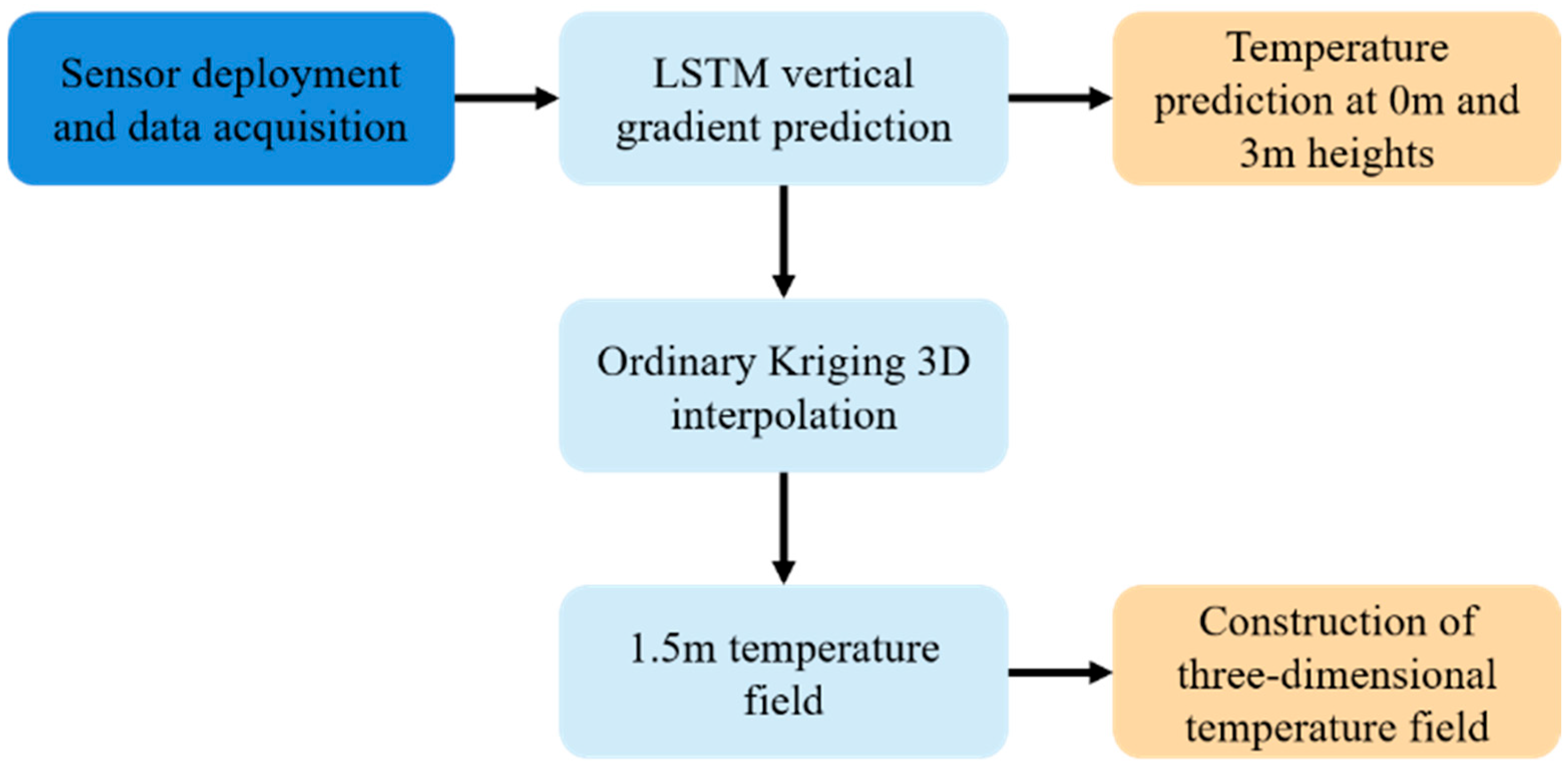
We discretized the domain on a regular (x, y, z) grid and, at each time step, performed three-dimensional ordinary kriging (3D-OK) on the temperature observations to obtain a gridded 3D temperature field. Repeating this for all 48 time steps yielded the daily spatiotemporal temperature sequence for the greenhouse. The modeling workflow is summarized in Figure 3.

4. Experimental Results and Analysis

4.1. Deep Learning Algorithm Model Selection

To evaluate the performance of different deep learning architectures in greenhouse temperature modeling, we compared the LSTM, GRU, Transformer, and TFT models across multiple metrics (summarized in Table 6). In terms of fitting accuracy, the coefficient of determination (R2) for LSTM ranges from 0.9796 to 0.9852, which is comparable to or even superior to those of GRU (0.9771–0.9844), Transformer (0.9811–0.9849), and TFT (0.9813–0.9847), indicating strong explanatory power for temperature time-series variations. For prediction errors, LSTM exhibits a root mean square error (RMSE) range of 0.5827–0.6761, narrower and lower than that of GRU (0.5962–0.7140), Transformer (0.5835–0.7109), and TFT (0.5866–0.7093), suggesting smaller deviations between predicted and actual values. Although the mean absolute error (MAE) of Transformer shows a slightly lower bound, LSTM’s MAE (0.4230–0.4657) remains competitive and well-aligned with other error indicators.
Beyond accuracy, LSTM also demonstrates advantages in training efficiency and stability. It requires only 0.54 min for training, significantly outperforming GRU (0.69 min), Transformer (0.64 min), and TFT (0.72 min), thus enabling faster modeling for real-time greenhouse environmental management. Moreover, the standard deviation of RMSE (σRMSE), a measure of model stability during repeated training, is 0.2929 for LSTM—substantially smaller than that of Transformer (0.5022), GRU (0.3599), and TFT (0.3568)—indicating more robust and consistent prediction performance.
Collectively, the LSTM model balances fitting accuracy, error control, training efficiency, and stability, making it the most suitable deep learning architecture for greenhouse temperature field modeling in this study.

4.2. Evaluation Based on the LSTM Vertical-Gradient Model

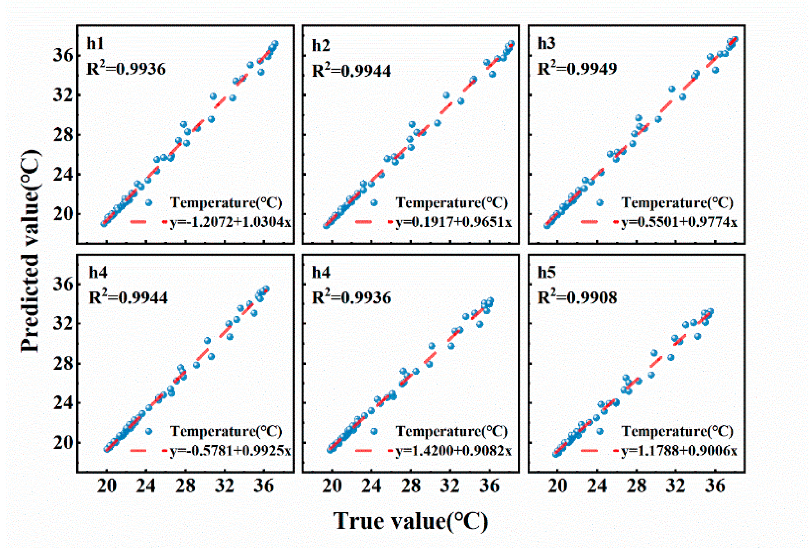
The dataset was split into training, validation, and test sets in an 8:1:1 ratio. The LSTM achieved R2 = 0.9786, MSE = 0.4823 °C, RMSE = 0.6945 °C, and MAE = 0.4561 °C, indicating strong predictive accuracy and effective capture of greenhouse temperature dynamics. To assess vertical applicability, predictions were regressed against measurements from six height-specific sensors (h1–h6) (Figure 4), all yielding R2 > 0.99 with slopes and intercepts close to the 1:1 line, confirming high agreement between predicted and observed temperatures.
To further evaluate model robustness, residual distributions were examined across different meteorological conditions and time intervals. The model maintained consistent accuracy under both sunny and cloudy conditions, with no significant bias between daytime and nighttime predictions. Outliers were defined as instances with absolute errors exceeding 1.5 °C, accounting for less than 2% of all samples. Most of these cases corresponded to transient microclimatic fluctuations near ventilation openings or brief sensor anomalies, rather than systematic prediction errors.
Overall, these results demonstrate that the LSTM exhibits strong vertical generalization and stable performance across varying environmental conditions, accurately reproducing temperature variation within the greenhouse air column.

4.3. Validation of Vertical Extrapolation and LSTM–Kriging Integration

To evaluate the reliability of the proposed hybrid LSTM–Kriging framework for vertical temperature extrapolation, we designed a vertical-holdout experiment. For each of the 12 temporal snapshots, all measurements at the top height layer (z = 3.0 m) were excluded during model fitting and subsequently predicted.
Three modeling schemes were compared:
(1)
Trend-only (LSTM)—direct extrapolation using the LSTM-predicted vertical gradient;
(2)
Kriging-only (3D OK)—purely spatial interpolation based on the remaining observed heights; and
(3)
Trend + Residual Kriging—a combination of LSTM trend and kriged residuals.
The aggregated validation results (Table 7) demonstrate that the Trend-only approach yields large errors (RMSE = 3.59 °C, MAE = 2.94 °C), showing that temporal prediction alone is insufficient for spatial extrapolation. The Kriging-only approach improves accuracy substantially (RMSE = 0.48 °C, MAE = 0.29 °C). The combined Trend + Residual Kriging approach achieves the lowest RMSE (0.46 °C) and reduces systematic bias from −0.166 °C to −0.031 °C.
Paired Wilcoxon tests indicate that the hybrid approach significantly outperforms both baselines (p < 0.01). Although the absolute RMSE gain over kriging-only is modest (~0.02 °C), the bias reduction and improved consistency across vertical layers confirm the complementary nature of the LSTM and kriging components.

4.4. Analysis of Model Applicability Under Different Weather Conditions

To assess the robustness and applicability of the 3D temperature field model across different meteorological regimes, two representative scenarios—sunny and rainy days—were analyzed, corresponding to the typical operational extremes in greenhouse conditions. Sunny days, characterized by strong solar radiation, induce large intra-day temperature fluctuations and strong vertical gradients, whereas rainy days, with weak insolation and high humidity, limit internal heat exchange and represent a more thermally stable state.
For each regime, a 3D ordinary kriging (3D-OK) model was constructed using 54 in-greenhouse temperature measurements and evaluated at 12:00. Under sunny conditions, temperatures ranged from 30.26 to 36.50 °C (σ = 1.65 °C). A spherical semivariogram provided the best fit (nugget = 0.271, sill = 2.438, range = 1.0). Leave-one-out cross-validation (LOOCV) yielded RMSE = 1.763 °C, MAE = 1.456 °C, and bias = 0.042 °C, reflecting greater spatial heterogeneity and thus higher interpolation uncertainty. Under rainy conditions, temperatures ranged from 28.78 to 34.10 °C (σ = 1.47 °C). A spherical model again fitted best (nugget = 0.215, sill = 1.939, range = 1.0), and LOOCV achieved RMSE = 1.283 °C, MAE = 1.055 °C, and bias = 0.019 °C—indicating more uniform spatial structure and higher prediction accuracy than under sunny conditions.
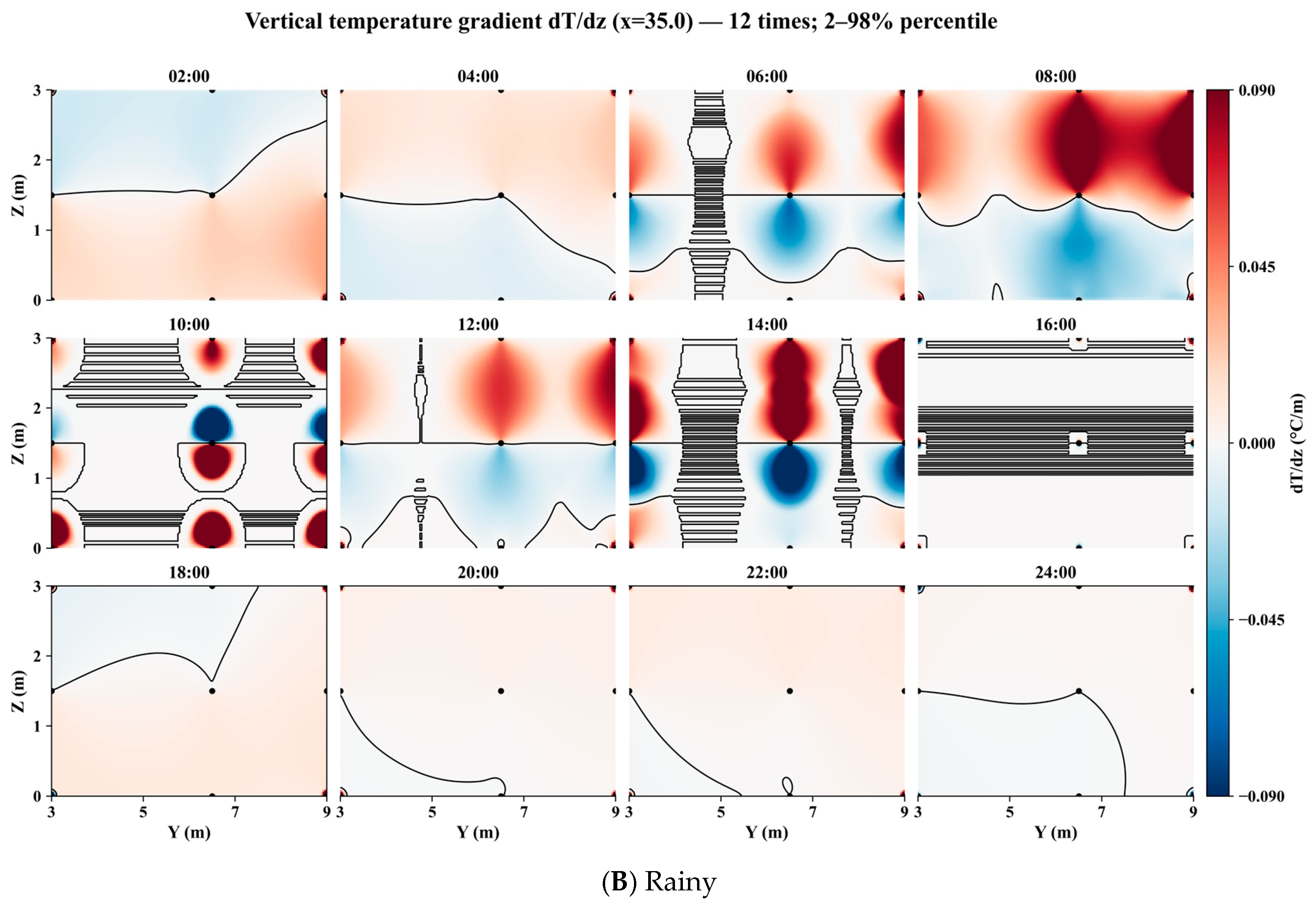
To further capture the diurnal and vertical dynamics, we reconstructed the greenhouse temperature field from 02:00 to 24:00 at 2 h intervals (Figure 5 and Figure 6). Figure 5A,B show the vertical temperature-gradient distributions (dT/dz) at x = 35.0 m for sunny and rainy days, respectively. On sunny days, strong positive gradients (red patches, 12:00–14:00) correspond to rapid upper-air heating, with values ranging between −0.1769 and 0.1769 °C m−1. On rainy days, gradient magnitudes are smaller (−0.090 to 0.090 °C m−1) and more homogeneous, confirming suppressed vertical stratification under weak solar input.
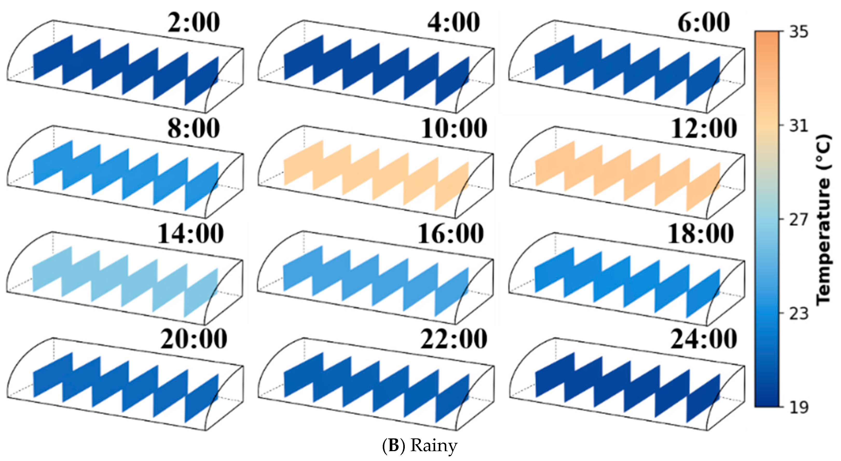
Figure 6A,B illustrate the 3D temperature field evolution for the same diurnal cycle. On sunny days, temperatures fluctuate widely (18–39 °C) with distinct warm zones expanding between 10:00 and 16:00, whereas on rainy days, the range narrows (19–35 °C) and color transitions are smoother. Quantitatively, averaged LOOCV errors across three representative time periods—morning (08:00–10:00), afternoon (12:00–16:00), and evening (18:00–22:00)—were RMSE = 1.28, 1.76, and 1.35 °C on sunny days versus 1.03, 1.29, and 1.12 °C on rainy days, respectively. These results confirm that while error magnitudes increase during peak radiation hours, they remain within 2 °C, validating the model’s stability across diurnal cycles.
The 2 h temporal resolution was selected as a balance between temporal detail and model stability: sensitivity analysis using 1 h data yielded only marginal RMSE improvement (<0.05 °C) but significantly increased computational cost and visual clutter, indicating that 2 h intervals are sufficient to resolve dominant diurnal trends.
In addition to mean temperature maps, the kriging variance fields were examined to evaluate uncertainty. Variance values peaked near boundary regions and decreased toward sensor-dense zones, with mean normalized kriging variance below 6% of the sill for both regimes, supporting the reliability of the spatial predictions.
Overall, the 3D temperature field model effectively distinguishes spatiotemporal dynamics under contrasting meteorological regimes. Sunny days exhibit stronger gradients, higher temperature peaks, and greater uncertainty, whereas rainy days show damped variability and smoother distributions. These patterns, quantified by cross-validation metrics and variance analysis, provide both visual and statistical evidence supporting the model’s robustness and its potential for weather-adaptive greenhouse control strategies.

5. Discussion

This study addresses the pronounced spatial heterogeneity of winter thermal conditions in solar greenhouses in northern China. We introduce and validate a 3D temperature field reconstruction framework that couples LSTM-based vertical-gradient prediction with three-dimensional ordinary kriging (3D-OK). Under sparse-sensor deployments, the method reconstructs spatiotemporal temperature fields for sunny and rainy regimes, capturing their distributional differences. The approach supports precise thermal regulation in protected agriculture via a 3D temperature field framework and provides a blueprint for low-cost, high-fidelity digital-twin greenhouse models.
The LSTM’s superior performance stems from its gating architecture, which effectively captures long-range dependencies in non-stationary time series. Compared with GRU, Transformer, and Temporal Fusion Transformer (TFT), LSTM shows lower performance variance across repeated training runs, making it well-suited to greenhouse temperature series influenced by both diurnal periodicity and slow trends. This is consistent with recent studies highlighting LSTM’s advantages in agricultural environmental forecasting and energy management [31,32]. Furthermore, LSTM provides high computational efficiency for time-series inference, enabling real-time operation on edge devices. This meets the demand for rapid on-site responses in controlled-environment agriculture (CEA) [33].
Relative to prior work, this study advances the state of the art in two key respects. First, prior studies have largely analyzed 2D temperature fields at a single height [34] or reconstructed spatial patterns using dense sensor networks [2], limiting dimensional fidelity or incurring high hardware costs. We reduce hardware requirements by combining sparse-sensor deployments with LSTM-based vertical-gradient prediction, enabling temperature estimation across the full 0–3 m vertical domain. Second, by coupling deep learning with geostatistical interpolation, we reconcile temporal dynamics with spatial continuity, providing a novel framework for modeling in controlled-environment agriculture (CEA). This aligns with recent trends toward interdisciplinary method integration [35].
From an application standpoint, access to all-weather, high-resolution 3D temperature fields directly supports intelligent, weather-adaptive greenhouse environmental control. On sunny days, pronounced peaks and large intra-day fluctuations warrant coordinated shading and ventilation to mitigate crop heat stress, whereas on rainy days, smaller temperature gradients and slower cooling justify delayed ventilation and reduced heating intensity to conserve energy. These recommendations are consistent with established greenhouse control strategies [36].
This study has several limitations. First, data were collected over a single month, omitting intra-annual and seasonal variability; consequently, cross-seasonal generalization remains to be validated. Preliminary tests using adjacent-month data indicated an average prediction bias of approximately 0.8–1.2 °C, suggesting moderate seasonal dependence. Second, three-dimensional ordinary kriging (3D-OK) assumes spatial stationarity, whereas greenhouses can exhibit non-stationarity under extreme weather or localized heating, potentially degrading local predictive accuracy. Additionally, while an isotropic variogram assumption was adopted due to limited sampling density, we acknowledge that greenhouse airflow often exhibits anisotropic patterns (e.g., longitudinal vs. vertical convection). Future work will incorporate anisotropic and non-stationary kriging formulations to capture such directional dependencies more accurately. Third, we modeled temperature alone, neglecting interactions with humidity, wind speed, and CO2, which limits in-depth analysis of microclimate coupling mechanisms.
Compared with traditional models such as linear regression, ARIMA, or energy-balance approaches, the LSTM demonstrates superior nonlinear fitting ability and temporal memory. However, its data dependency and limited interpretability may constrain generalization under unseen conditions, especially when training samples are limited. Furthermore, the hybrid LSTM–3D-OK framework, while effective, inherits kriging’s stationary assumption and sensitivity to sparse measurements.
Recent studies have explored combining deep learning and spatial interpolation, such as CNN–kriging [37], which provides valuable context for our approach. Future work should enhance applicability and robustness by collecting multimodal environmental data, incorporating non-stationary kriging and co-kriging, and leveraging machine-learning methods for spatiotemporal modeling [38]. Research can proceed along three directions: (1) expand data collection to cover a full year and extreme events to strengthen cross-seasonal generalization; (2) incorporate multimodal variables (humidity, wind speed, CO2) to enable multi-factor coupled prediction and elucidate greenhouse microclimate dynamics; and (3) explore advanced spatial statistical methods—non-stationary kriging and co-kriging—coupled with multi-task deep learning frameworks to improve applicability and predictive accuracy in complex, heterogeneous environments.
In summary, under sparse-sensor deployments, the proposed framework—coupling LSTM-based vertical-gradient prediction with three-dimensional ordinary kriging (3D-OK)—efficiently and accurately reconstructs greenhouse 3D temperature fields, offering a practical paradigm for environmental modeling in protected agriculture. Future work will pursue multivariate coupled prediction, strengthen cross-seasonal generalization, and deepen integration with intelligent greenhouse control systems to advance digitalization and intelligent development in protected agriculture. Additionally, since this study focused on methodological validation rather than agronomic assessment, future work will incorporate crop growth and yield measurements to evaluate the practical agronomic benefits of reconstructed temperature fields.

6. Conclusions

This study proposes an integrated framework for reconstructing three-dimensional (3D) temperature fields in solar greenhouses by coupling long short-term memory (LSTM)–based vertical-gradient prediction with three-dimensional ordinary kriging (3D-OK). The framework enables continuous spatiotemporal mapping of greenhouse temperature distributions under sparse-sensor deployments, providing a potential foundation for precision environmental regulation and digital-twin applications in protected agriculture.
Experimental results show that the LSTM achieved stable performance for multi-height temperature prediction (R2 ≈ 0.98 on the test set) and effectively captured both diurnal variation and vertical temperature gradients. When combined with 3D-OK interpolation, the reconstructed temperature fields exhibited physically consistent spatial structures and realistic thermal patterns across different weather conditions, verifying the feasibility of the proposed method.
The proposed LSTM–3D-OK approach offers a proof-of-concept solution for cost-effective 3D temperature reconstruction under practical sensor constraints. However, certain limitations should be acknowledged: the dataset covers only a short observation period, and seasonal or inter-annual variations were not examined. Future studies should extend the method to longer time spans, multiple greenhouse configurations, and real-time control scenarios to further validate generalizability.
Overall, the study demonstrates that integrating data-driven vertical-gradient modeling with spatial interpolation can effectively reproduce key features of greenhouse thermal heterogeneity while maintaining feasibility under limited sensor conditions.

Author Contributions

Conceptualization, Z.Z. and X.L.; methodology, Z.Z. and X.L.; software, X.Z. and Z.G.; formal analysis, Z.Z. and Z.G.; data curation, Z.Z. and Y.L.; writing—original draft preparation, Z.Z. and X.Z.; writing—review and editing, Z.Z.; visualization, X.L.; supervision, X.F. and X.H.; project administration, L.L.; funding acquisition, W.Z. All authors have read and agreed to the published version of the manuscript.

Funding

This research received no external funding.

Data Availability Statement

The raw data supporting the conclusions of this article will be made available by the authors on request.

Conflicts of Interest

The authors declare no conflicts of interest.

References

  1. Singh, K.A.P.; Goutam, P.K.; Xaxa, S.; Nasima, S.P.; Panotra, N.; Rajesh, G. The role of greenhouse technology in streamlining crop production. J. Exp. Agric. Int. 2024, 46, 776–798. [Google Scholar] [CrossRef]
  2. Xiao, Y.; Gong, J.; Wang, Y.; Wang, C. Intelligent agricultural greenhouse control system based on internet of things and machine learning. In Proceedings of the 2025 International Conference on Machine Learning and Neural Networks, Suzhou, China, 18–20 April 2025; pp. 292–300. [Google Scholar]
  3. Boersma, S.; Cheng, X. A Bayesian Neural ODE for a Lettuce Greenhouse. In Proceedings of the 2024 IEEE Conference on Control Technology and Applications (CCTA), Newcastle upon Tyne, UK, 21–23 August 2024; pp. 782–786. [Google Scholar]
  4. Boulard, T.; Wang, S. Greenhouse crop transpiration simulation from external climate conditions. Agric. For. Meteorol. 2000, 100, 25–34. [Google Scholar] [CrossRef]
  5. Körner, O.S.G.V.; Van Straten, G. Decision support for dynamic greenhouse climate control strategies. Comput. Electron. Agric. 2008, 60, 18–30. [Google Scholar] [CrossRef]
  6. Tong, G.; Christopher, D.M.; Li, B. Numerical modelling of temperature variations in a Chinese solar greenhouse. Comput. Electron. Agric. 2009, 68, 129–139. [Google Scholar] [CrossRef]
  7. Abou-Mehdi-Hassani, F.; Zaguia, A.; Ait Bouh, H.; Mkhida, A. Systematic literature review of smart greenhouse monitoring. SN Comput. Sci. 2025, 6, 95. [Google Scholar] [CrossRef]
  8. Săcăleanu, D.-I.; Matache, M.-G.; Roșu, Ș.-G.; Florea, B.-C.; Manciu, I.-P.; Perișoară, L.-A. IoT-enhanced decision support system for real-time greenhouse microclimate monitoring and control. Technologies 2024, 12, 230. [Google Scholar] [CrossRef]
  9. Bhujel, A.; Basak, J.K.; Khan, F.; Arulmozhi, E.; Jaihuni, M.; Sihalath, T.; Lee, D.; Park, J. Sensor systems for greenhouse microclimate monitoring and control: A review. J. Biosyst. Eng. 2020, 45, 341–361. [Google Scholar] [CrossRef]
  10. Cheng, X.; Li, D.; Shao, L.; Ren, Z. A virtual sensor simulation system of a flower greenhouse coupled with a new temperature microclimate model using three-dimensional CFD. Comput. Electron. Agric. 2021, 181, 105934. [Google Scholar] [CrossRef]
  11. Cai, H.; Liang, Z.; Lyu, Y.; Qin, Y. Numerical Simulation Analysis of Large-Scale Three-Dimensional Planting Greenhouse Based on Orthogonal Test Method. J. Appl. Math. Phys. 2025, 13, 914–932. [Google Scholar] [CrossRef]
  12. Fatnassi, H.; Bournet, P.E.; Boulard, T.; Roy, J.C.; Molina-Aiz, F.D.; Zaaboul, R. Use of computational fluid dynamic tools to model the coupling of plant canopy activity and climate in greenhouses and closed plant growth systems: A review. Biosyst. Eng. 2023, 230, 388–408. [Google Scholar] [CrossRef]
  13. Rezvani, S.M.E.D.; Shamshiri, R.R.; Hameed, I.A.; Abyane, H.Z.; Godarzi, M.; Momeni, D.; Balasundram, S.K. Greenhouse crop simulation models and microclimate control systems, a review. In Next-Generation Greenhouses for Food Security; IntechOpen: London, UK, 2021. [Google Scholar]
  14. Li, X.; Zhang, L.; Wang, X.; Liang, B. Forecasting greenhouse air and soil temperatures: A multi-step time series approach employing attention-based LSTM network. Comput. Electron. Agric. 2024, 217, 108602. [Google Scholar] [CrossRef]
  15. Liu, Y.; Li, D.; Wan, S.; Wang, F.; Dou, W.; Xu, X.; Qi, L. A long short-term memory-based model for greenhouse climate prediction. Int. J. Intell. Syst. 2022, 37, 135–151. [Google Scholar] [CrossRef]
  16. Arnaud, S.E.; Calisti, M.; Polydoros, A. Data-Driven Greenhouse Climate Regulation in Lettuce Cultivation Using BiLSTM and GRU Predictive Control. arXiv 2025, arXiv:2507.21669. [Google Scholar]
  17. Jung, D.H.; Kim, H.S.; Jhin, C.; Kim, H.J.; Park, S.H. Time-serial analysis of deep neural network models for prediction of climatic conditions inside a greenhouse. Comput. Electron. Agric. 2020, 173, 105402. [Google Scholar] [CrossRef]
  18. Vaswani, A.; Shazeer, N.; Parmar, N.; Uszkoreit, J.; Jones, L.; Gomez, A.N.; Kaiser, L.; Polosukhin, I. Attention is all you need. arXiv 2017, arXiv:1706.03762. [Google Scholar]
  19. Feng, G.; Zhang, L.; Ai, F.; Zhang, Y.; Hou, Y. An improved temporal fusion transformers model for predicting supply air temperature in high-speed railway carriages. Entropy 2022, 24, 1111. [Google Scholar] [CrossRef]
  20. Seri, E.; Petitta, M.; Cornaro, C. Sustainable Greenhouse Management: A Comparative Analysis of Recurrent and Graph Neural Networks. arXiv 2025, arXiv:2502.17371. [Google Scholar] [CrossRef]
  21. Yin, H.; Wang, K.; Zeng, J.; Pang, Z. CFD Analysis and Optimization of a Plastic Greenhouse with a Semi-Open Roof in a Tropical Area. Agronomy 2024, 14, 876. [Google Scholar] [CrossRef]
  22. Guo, Z.; Feng, L. Multi-step prediction of greenhouse temperature and humidity based on temporal position attention LSTM. Stoch. Environ. Res. Risk Assess. 2024, 38, 4907–4934. [Google Scholar] [CrossRef]
  23. Shasteen, K.C.; Kacira, M. Predictive modeling and computer vision-based decision support to optimize resource use in vertical farms. Sustainability 2023, 15, 7812. [Google Scholar] [CrossRef]
  24. Panda, M.; Khilar, P.M. Distributed self fault diagnosis algorithm for large scale wireless sensor networks using modified three sigma edit test. Ad Hoc Netw. 2015, 25, 170–184. [Google Scholar] [CrossRef]
  25. Blu, T.; Thévenaz, P.; Unser, M. Linear interpolation revitalized. IEEE Trans. Image Process. 2004, 13, 710–719. [Google Scholar] [CrossRef] [PubMed]
  26. Benesty, J.; Chen, J.; Huang, Y.; Cohen, I. Pearson correlation coefficient. In Noise Reduction in Speech Processing; Springer: Berlin/Heidelberg, Germany, 2009; pp. 1–4. [Google Scholar]
  27. Bhanja, S.; Das, A. Impact of data normalization on deep neural network for time series forecasting. arXiv 2018, arXiv:1812.05519. [Google Scholar]
  28. Lim, B.; Arık, S.Ö.; Loeff, N.; Pfister, T. Temporal fusion transformers for interpretable multi-horizon time series forecasting. Int. J. Forecast. 2021, 37, 1748–1764. [Google Scholar] [CrossRef]
  29. Cho, K.; Van Merriënboer, B.; Gulcehre, C.; Bahdanau, D.; Bougares, F.; Schwenk, H.; Bengio, Y. Learning phrase representations using RNN encoder-decoder for statistical machine translation. arXiv 2014, arXiv:1406.1078. [Google Scholar] [CrossRef]
  30. Xia, H.; Liu, Y.; Gong, Y.; Ren, N.; Jin, J. Comparative study on greenhouse three-dimensional temperature field construction methods based on spatial interpolation. J. Chin. Agric. Mech. 2025, 46, 176–182. [Google Scholar] [CrossRef]
  31. Gharghory, S.M. Deep network based on long short-term memory for time series prediction of microclimate data inside the greenhouse. Int. J. Comput. Intell. Appl. 2020, 19, 2050013. [Google Scholar] [CrossRef]
  32. Esparza-Gómez, J.M.; Guerrero-Osuna, H.A.; Ornelas-Vargas, G.; Luque-Vega, L.F. RNN-LSTM Applied in a Temperature Prediction Model for Greenhouses. Res. Comput. Sci. 2021, 150, 31–41. [Google Scholar]
  33. Guillén, M.A.; Llanes, A.; Imbernón, B.; Martínez-España, R.; Bueno-Crespo, A.; Cano, J.C.; Cecilia, J.M. Performance evaluation of edge-computing platforms for the prediction of low temperatures in agriculture using deep learning. J. Supercomput. 2021, 77, 818–840. [Google Scholar] [CrossRef]
  34. Balendonck, J.; Os, E.V.; Schoor, R.V.D.; Tuijl, B.V.; Keizer, L.C.P. Monitoring spatial and temporal distribution of temperature and relative humidity in greenhouses based on wireless sensor technology. In Proceedings of the International Conference on Agricultural Engineering, Clermont-Ferrand, France, 6–8 September 2010. [Google Scholar]
  35. Wang, Y.; Yuan, F.; Cammarano, D.; Liu, X.; Tian, Y.; Zhu, Y.; Cao, W.; Cao, Q. Integrating machine learning with spatial analysis for enhanced soil interpolation: Balancing accuracy and visualization. Smart Agric. Technol. 2025, 11, 101032. [Google Scholar] [CrossRef]
  36. Shi, J.; Wang, H.; Wang, J. Cfd simulation study on the cooling characteristics of shading and natural ventilation in greenhouse of a botanical garden in shanghai. Sustainability 2023, 15, 3056. [Google Scholar] [CrossRef]
  37. Hua, Y.; Zhao, X.; Sun, W.; Sun, Q. Satellite-Based Reconstruction of Atmospheric CO2 Concentration over China Using a Hybrid CNN and Spatiotemporal Kriging Model. Remote Sens. 2024, 16, 2433. [Google Scholar] [CrossRef]
  38. Hengl, T.; Nussbaum, M.; Wright, M.N.; Heuvelink, G.B.; Gräler, B. Random forest as a generic framework for predictive modeling of spatial and spatio-temporal variables. PeerJ 2018, 6, e5518. [Google Scholar] [CrossRef] [PubMed]
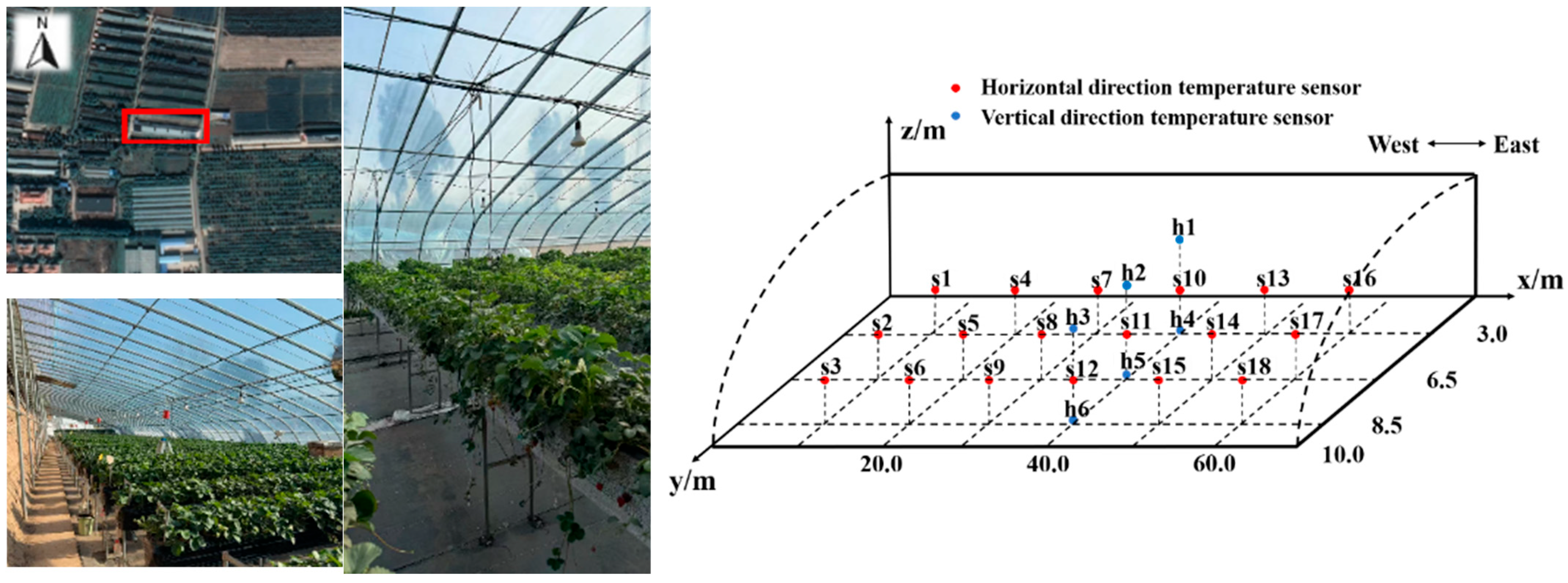
Figure 1. Sensor Layout and Coordinate System (Including Scale and Azimuth).
Agriculture 15 02222 g001
Figure 2. Workflow of the LSTM-based temperature prediction model. The model processes a 12-step sequence containing three features and outputs six temperature predictions corresponding to distinct sensor positions.
Agriculture 15 02222 g002
Figure 3. Flowchart of the 3D Greenhouse Temperature Field Reconstruction Method. This diagram illustrates the process of constructing a 3D greenhouse temperature field, encompassing the following steps: 1.5m plane temperature interpolation, temperature extrapolation based on vertical gradients, and generation of the complete temperature field via 3D ordinary Kriging interpolation.
Agriculture 15 02222 g003
Figure 4. Linear regression results between predicted and measured values for sensors at six different locations.
Agriculture 15 02222 g004
Figure 5. Vertical temperature-gradient distribution at (x = 35.0 m) in a solar greenhouse under sunny (A) and rainy (B) conditions (12 time points from 02:00 to 24:00; data filtered to the 2–98% percentile).
Agriculture 15 02222 g005aAgriculture 15 02222 g005b
Figure 6. Three-dimensional temperature field simulation results inside the greenhouse from 2:00 to 24:00 (every 2 h) under different weather conditions. (A) Clear weather conditions, temperature range 18–39 °C. (B) Rainy weather conditions, temperature range 19–35 °C.
Agriculture 15 02222 g006aAgriculture 15 02222 g006b
Table 1. Summary of representative greenhouse temperature modeling studies with corresponding advantages and limitations.
CategoryRepresentative StudiesAdvantagesLimitations
Sensor-based monitoringIoT deployments and WSN reviews [7,8]; sensor-system review [9]Provide real-time, in situ high-fidelity measurements; capture local microclimate and transient events; enable closed-loop controlHigh installation and maintenance costs for dense coverage; sparse networks miss 3D continuity of temperature field; sensors require calibration and can drift
Numerical simulation (CFD)CFD ventilation/microclimate studies and method reviews [12,21]Resolve three-dimensional airflow and heat-transfer processes; test ventilation/roof/vent configurations and canopy effects; useful for design and what-if analysesHigh computational cost; results sensitive to mesh, turbulence model and boundary conditions; requires experimental data for calibration/validation
Statistical/data-driven modelingMulti-step and attention/LSTM forecasting, hybrid ML studies [12,22]Efficient for short-term forecasting and real-time applications; can learn complex nonlinear relations and act as surrogates for control; lower computational cost than full CFDOften trained on limited sensor locations (spatial extrapolation challenges); may not explicitly represent physical processes or 3D spatial structure; generalization depends on training-data representativeness
Table 2. Horizontal Temperature Sensor Coordinate Points.
Temperature Sensor
Coordinatess1s2s3s4s5s6s7s8s9s10s11s12s13s14s15s16s17s18
x555151515252525353535454545555555
y36.5936.5936.5936.5936.5936.59
z1.51.51.51.51.51.51.51.51.51.51.51.51.51.51.51.51.51.5
Table 3. Vertical Temperature Sensor Coordinate Points.
Temperature Sensor
Coordinatesh1h2h3h4h5h6
x353535353535
y36.5936.59
z333000
Table 4. Analysis of Pearson Correlation Results.
Temperature Pointh1h2h3h4h5h6
s100.9973 ***0.9941 ***0.9937 ***0.9867 ***0.9817 ***0.9758 ***
s110.9977 ***0.9973 ***0.9981 ***0.9846 ***0.9829 ***0.9788 ***
s1209960 ***0.9965 ***0.9977 ***0.9828 ***0.9820 ***0.9772 ***
Note: *** indicates p < 0.001.
Table 5. Comparison of variogram models by LOOCV (N = 648).
Variogram ModelRMSE (°C)MAE (°C)R2n_Valid
Spherical0.763530.503120.96655648
Exponential0.761350.501530.96674648
Gaussian0.766580.503170.96628648
Table 6. Evaluation and computational efficiency metrics for different models in the greenhouse temperature prediction task.
ModelR2RMSE (°C)MAE (°C)Training Time (Min)Stability (σRMSE)
LSTM(0.9796, 0.9852)(0.5827, 0.6761)(0.4230, 0.4657)0.540.2929
GRU(0.9771, 0.9844)(0.5962, 0.7140)(0.4018, 0.4651)0.690.3599
Transformer(0.9811, 0.9849)(0.5835, 0.7109)(0.3826, 0.4479)0.640.5022
TFT(0.9813, 0.9847)(0.5866, 0.7093)(0.3886, 0.4570)0.720.3568
Table 7. Vertical-holdout validation results (N = 216).
MethodNRMSE (°C)MAE (°C)Bias (°C)
Trend-only (LSTM)2163.59482.9367−0.2939
Kriging-only (3D-OK)2160.479660.29367−0.1660
Trend + Residual Kriging2160.455580.33987−0.03148
Disclaimer/Publisher’s Note: The statements, opinions and data contained in all publications are solely those of the individual author(s) and contributor(s) and not of MDPI and/or the editor(s). MDPI and/or the editor(s) disclaim responsibility for any injury to people or property resulting from any ideas, methods, instructions or products referred to in the content.