Abstract
The growth environment of corps requires necessary improvements by Chinese solar greenhouses with Pad–Fan Cooling (PFC) systems for reducing their high temperatures in summer. Although computational fluid dynamics (CFD) could dynamically display the changes in humidity, temperature, and wind speed in solar greenhouses, its computational efficiency and accuracy are relatively low. In addition, the use of PFC systems can cool down solar greenhouses in summer, but they will also cause excessive humidity inside the greenhouses, thereby reducing the production efficiency of crops. Most existing studies only verify the effectiveness of a single machine learning (such as ARMA or ARIMA) or deep learning model (such as LSTM or TCN), lacking systematic comparison of different models. In the current study, two machine learning algorithms and three deep learning algorithms were used for their ability to predict a PFC system’s cooling effect, including on humidity, temperature, and wind speed, which were examined using Auto Regression Moving Average (ARMA), Autoregressive Integrated Moving Average (ARIMA), Long Short-Term Memory (LSTM), Time Convolutional Network (TCN), and Glavnoe Razvedivatelnoe Upravlenie (GRU), respectively. These results show that deep learning algorithms are significantly more effective than traditional machine learning algorithms in capturing the complex nonlinear relationships and spatiotemporal changes inside solar greenhouses. The LSTM model achieves R2 values of 0.918 for temperature, 0.896 for humidity, and 0.849 for wind speed on the test set. TCN showed strong performance in identifying high-frequency fluctuations and extreme nonlinear features, particularly in wind speed prediction (test set R2 = 0.861). However, it exhibited limitations in modeling certain temperature dynamics (e.g., T6 test set R2 = 0.242) and humidity evaporation processes (e.g., T7 training set R2 = −0.856). GRU delivered excellent performance, achieving a favorable balance between accuracy and efficiency. It attained the highest prediction accuracy for temperature (test set R2 = 0.925) and humidity (test set R2 = 0.901), and performed only slightly worse than TCN in wind speed prediction. In summary, deep learning models, particularly GRU, offer more reliable methodological support for greenhouse microclimate prediction, thereby facilitating the precise regulation of cooling systems and scientifically informed crop management.
1. Introduction
Chinese solar greenhouses (CSGs) are regarded as a unique and cost-effective greenhouse type in China, featuring excellent thermal insulation and high energy efficiency, which enables winter vegetable production without auxiliary heating, even when the monthly average temperature during the coldest three months drops below −10 °C [1,2]. However, this superior thermal performance presents a contrasting challenge during warmer periods. During summer months, the internal temperatures of CSGs frequently exceed 50 °C due to intense solar radiation, leading to stunted growth or even crop mortality [3]. High temperatures and humidity in greenhouses could severely limit production by reducing yields and compromising produce quality during extended periods. However, correct climate control using various cooling methods enables sustained crop cultivation in warm seasons, particularly crucial for heat-sensitive vegetables such as tomatoes, cucumbers, peppers, and lettuce, which exhibit growth declines when temperatures exceed their optimal 29–30 °C range, making cooling system implementation essential for successful summer cultivation [4,5]. Various greenhouse cooling methods have been developed, with shading and natural ventilation being the most common methods of temperature control, although their cooling effectiveness remains limited. Among existing greenhouse cooling technologies, evaporative cooling systems have proven to be the most effective solution [6]. The pad–fan configuration represents the most widely implemented form of this technology. Pad–Fan Cooling (PFC) systems have emerged as an effective solution for summer overheating in greenhouses due to their efficient and stable cooling performance. When properly designed, these systems could reduce air temperature by 5–12 °C and create more favorable conditions for crop growth. PFC systems are widely used in greenhouse temperature control and have high cooling efficiency, but they have several obvious limitations: non-uniform temperature distribution within the greenhouse, and substantial installation and maintenance costs [7]. These limitations not only impact the overall performance of the cooling systems, but also pose significant challenges for growers in terms of cost management and crop uniformity. Thus, the spatio−temporal distribution of temperature, humidity, and airflow under Pad–Fan Cooling operation is crucial for optimizing greenhouse cooling strategies. Traditional approaches to optimizing PFC systems relies heavily on computational fluid dynamics (CFD) simulations, which, although effective in modeling airflow and thermal distribution, suffer from high computational costs, complex boundary condition setups, and limited real-time applicability. Moreover, existing research mainly focuses on environmental simulations of empty greenhouses, leaving significant gaps in our understanding of crop−environment interaction mechanisms. Particularly for low-profile crops like strawberries, the mechanism by which canopy structures influence greenhouse microenvironments remains unclear, which hinders the optimal design of cooling systems. Meanwhile, existing studies analyzing greenhouse microclimates have shown insufficient attention to the role of soil. As a crucial component of greenhouse ecosystems, soil directly influences indoor temperature distribution through various heat exchange mechanisms such as thermal conduction and radiation within the air [8,9]. Additionally, its moisture evaporation process alters air humidity dynamics [10]. Specifically, soil surface temperature rises by absorbing solar radiation during the day and releasing stored heat at night, buffering extreme temperature fluctuations in the greenhouse [11]. However, the soil-mediated microclimate regulation and crop canopy structure further interact with each other to form a complex “soil−crop−microclimate” dynamic relationship. The mechanism of this process has not been fully revealed, which further hinders the accurate design of cooling systems. To address this gap, microclimate prediction has become a crucial component that bridges the interactions between soil, crops, and greenhouse micro-environments with practical greenhouse regulation. In solar greenhouses equipped with PFC systems, “microclimate prediction” refers to the quantitative forecasting of key environmental parameters such as temperature, humidity, and wind speed across spatial and temporal dimensions. In other words, its primary objective is to clarify how the micro-environment in greenhouses (including temperature, humidity, and wind speed) dynamically changes across different locations and time periods under various influencing factors such as PFC system operation, solar radiation, soil heat and moisture exchange, and crop–canopy interactions. This research provides theoretical foundations and data support for the precise regulation of cooling systems and scientific management of crops.
In recent years, the development of machine learning (ML) had provided new possibilities for predicting and optimizing greenhouse climates. Compared to traditional CFD methods, ML models could process real-time sensor data, capture complex relationships between environmental variables, and calculate higher computational efficiency. A multiple linear regression model was used to predict the evapotranspiration and transpiration of greenhouse tomatoes [12,13,14]. Photosynthetically active radiation, total radiation, day–night temperature and humidity, and leaf fresh weight were regarded as input variables to achieve precise irrigation and efficient utilization of water resources. Neural networks and multiple-regression models were introduced to predict the roof temperature and air humidity inside a half-daylight-temperature room [15,16,17]. The results show that neural networks have significantly improved prediction accuracy than multiple-regression models, demonstrating their potential for the intelligent prediction of greenhouse environments. A greenhouse environment model was constructed by using an online sparse least squares support vector machine regression model [18,19,20]. The indoor and outdoor temperatures were regarded as input variables, achieved low mean square error, and had a concise model structure. Compared to methods such as recursive weighted least squares estimation and Elman neural networks, this model exhibited higher prediction accuracy. This work provides a nonlinear modeling method suitable for online learning, which has practical value for the intelligent control of greenhouse environments. The greenhouse tomato transpiration prediction model was established based on the random forest algorithm [21,22]. The input variables included air temperature, relative humidity, light intensity, and relative leaf area index. The determination coefficients of the model in the seedling stage and flowering stage reached 0.9472 and 0.9654, respectively, and the prediction error was much lower than that of the BP neural network and GA–BP neural network. This indicated that the model has practical significance in precision irrigation management. A tomato yield prediction model was developed by combining recurrent neural networks and Time Convolutional Networks [23,24,25]. The model was trained by using greenhouse environmental parameters and historical yield data, with root mean square errors as low as 6.76–10.45 g/m2 on multiple test sets. The study also found that historical production information had the most significant impact on the prediction results. This method helps growers to develop management strategies scientifically. The greenhouse climate prediction model was proposed by using long short-term memory networks [26,27,28]. This model took into account six factors, including temperature, humidity, light, carbon dioxide concentration, air temperature, and soil moisture, and updated the data every 5 min. In practical applications in tomato, cucumber, and chili greenhouses, the model performed stably and maintains good predictive ability, even when encountering abnormal data, which is of great significance when there is a need to adjust the greenhouse environment in advance and ensure crop growth. A gated cyclic unit model was developed to predict the minimum temperature [29,30]. The model was trained by using monthly average minimum temperature data from over 30 years in the local area. The model had minimal errors during the testing phase, and was able to make reasonable predictions of the minimum temperature for the next year or more. This prediction method provides strong support for greenhouse temperature regulation. The ARMA model was used to predict the weekly harvest of sweet peppers [31,32,33]. Production data from previous weeks were incorporated into the model, which resulted in improved predictive performance over traditional reference models. For some varieties, the addition of environmental variables reduced the prediction error by 20%, which indicated that the method had certain practical value in greenhouse production arrangements. The trend of carbon dioxide emissions in greenhouses was analyzed by using ARIMA models, which shows that the model performs well in short-term forecasting and is helpful in evaluating changes in greenhouse effects [34,35]. Research is increasingly focusing on the application of machine learning in greenhouse environment prediction, but most studies only verify the effectiveness of a certain type of model separately without conducting a systematic comparative analysis. The summary of the literature is presented in Table 1.

Table 1.
Summary of the literature.
In the current study, the experimental microclimate data in CSG with PFC systems of Shenyang Agricultural University were utilized by two machine learning algorithms and three deep learning algorithms for their ability to predict a PFC system’s cooling effects, including humidity, temperature, and wind speed, which were ARMA, ARIMA, LSTM, TCN, and GRU, respectively; it was found that deep learning models such as TCN, GRU, and LSTM perform better in greenhouse climate prediction than traditional ARMA and ARIMA models. TCN, with its multi-scale receptive field of dilated convolution, has greater potential for capturing high-frequency fluctuations and extreme nonlinear relationships in temperature and humidity, and could better adapt to the spatial attenuation of airflow. LSTM balanced long- and short-term dependencies by gating mechanisms and exhibiting robustness. GRU simplified the gating structure of LSTM, ensuring accuracy while improving efficiency. Introducing multiple machine learning methods for joint prediction in the future is expected to further improve the accuracy and practicality of predictions.
Core Contributions of This Study: This study compares the two traditional algorithms (ARMA and ARIMA) with three deep learning algorithms (LSTM, TCN, and GRU) to address the lack of systematic comparisons of models in existing studies. It was found that the deep learning model equipped with PFC significantly outperformed the traditional model in predicting temperature, humidity, and wind speed in the CSG system.
Compared to the traditional model (which finds it difficult to deal with nonlinear fluctuations) and other deep learning models (TCN has limitations, and LSTM has high cost), GRU achieves an optimal balance between accuracy and efficiency (convergence is 30% faster than LSTM).
2. Methods and Materials
Figure 1 shows the research steps for predicting the microclimates of CSG with PFC systems. This framework consists of multi-sensor monitoring and machine learning forecasting. There are five main parts: (1) Preparing for microclimate monitoring. (2) Collecting and preprocessing data. (3) Building machine learning models. (4) Training, evaluating, and comparing multiple models. (5) Finding the best prediction model. Firstly, in the preparatory stage of the research, several measuring points were configured in the CSG. These points were marked for temperature (T1–T7), humidity (T1, T2, T3, T6, T7), and wind speed (T2, T6, T7). All instruments were calibrated and prepared, such as the ADCON temperature sensor, Testo45 anemograph, and multi-function temperature–humidity meter. The next part was data acquisition and preprocessing. With the installed sensors, microclimate data could be obtained, including temperature, humidity, and wind speed, which were subsequently preprocessed. Missing values were address by employing a min–max scaler for normalization and performing correlation testing to select the features. In the model construction stage, traditional statistical models (ARMA, ARIMA) and deep learning models (LSTM, TCN, GRU) were introduced. These models underwent processes such as data preprocessing adaptation, orthogonality verification, and feature engineering implementation, which is beneficial for fitting the CSG microclimate data. For the purposes of model training, evaluation, and comparison, the preprocessed data was utilized in conjunction with performance metrics (e.g., loss functions) and visualization techniques (e.g., loss curves and comparisons of sequence predictions). ARMA, ARIMA, LSTM, TCN, and GRU models were compared using R2 and root mean square error (RMSE). This checked how well they predict greenhouse microclimate variables. Finally, for optimal model identification, we consider both prediction accuracy and efficiency. From the compared models, we picked the best one (GRU, which is 30% faster and still accurate). This provided a reliable tool for predicting and managing greenhouse microclimates.
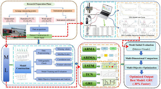
Figure 1.
Workflow for greenhouse microclimate prediction integrating multi-sensor monitoring and machine learning.
2.1. Experimental Greenhouse
The CSG is located at Shenyang Agricultural University in Shenyang, Liaoning Province (41°49′ N, 123°34′ E), specifically within Greenhouse No. 46, as shown in Figure 2 and Figure 3. This single-span greenhouse is oriented in a north–south direction, with a slight deviation of 7° west of due south, designed to maximize solar radiation capture during winter. The CSG has a total length of 60 m, a span of 10 m, a rear-wall height of 3.2 m, and a ridge height of 5 m, covering a total ground area of 480 m2. The greenhouse structure consists of four primary components: the front wall, side walls, rear slope, and foundation soil. The rear wall is consist of an inner brick wall, an expanded polystyrene (EPS) insulation layer, and an outer brick wall (240 mm thick solid clay bricks with 20 mm plaster on both surfaces). The rear slope is composed of wooden boards, an EPS insulation layer, cement, and a waterproof layer. The structure adopts an arched truss design that eliminates the need for supporting pillars, with its roof, gable walls, and front roof structure all covered with 0.1 mm thick polyethylene plastic film. A Pad–Fan Cooling system was installed for indoor temperature regulation, which consists of a galvanized aluminum alloy wet pad (dimensions: 3 m in length × 0.15 m in width × 1.5 m in height, with a total area of 4.5 m2), two negative-pressure fans (each with a diameter of 1.06 m, width of 0.4 m, power of 0.55 kW, blade speed of 650 rpm, and airflow rate of 38,000 m3/h), a horizontal centrifugal pump, a rectangular water tank (dimensions: 1 m in length × 0.5 m in width × 0.45 m in height, with a volume of 0.225 m3 or 225 L), and an control unit. Strawberries are grown in the greenhouse at a planting density of 8500 plants per hectare, arranged in rows oriented in the north–south direction. A thermal insulation curtain is operated daily (opened at 08:30 and closed at 16:30) to enhance temperature regulation between day and night.
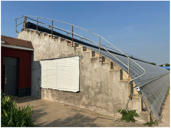
Figure 2.
External structure of the greenhouse.
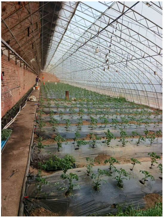
Figure 3.
Internal Structure of the greenhouse.
2.2. Experimental Methods
2.2.1. Experimental Apparatus
Indoor greenhouse temperatures at various positions were measured using ADCON instruments manufactured in the United States. These instruments have a measurement range from −40 °C to 120 °C and provide a high accuracy of ±0.2 °C. A multifunctional temperature and humidity meter was employed to measure indoor humidity within the CSG, offering a temperature measurement range from −30 °C to 50 °C (accuracy: ±1 °C) and a humidity measurement range of 0–100% RH. Wind speed at different indoor locations was assessed using a Testo 425 handheld thermal anemometer, which has a measurement range from 0 to 40 m/s, an accuracy of ±(0.2 m/s + 1.5% of the reading), and a resolution of 0.1 m/s. Outdoor temperature and humidity were monitored using the TRM−ZSF GPRS wireless remote control system developed by Jinzhou Sunshine Technology Co., Ltd. (based in Jinzhou City, China), capable of measuring humidity within the range of 0–90% RH and temperature from −25 °C to 70 °C. The external climate remained stable throughout the experimental period. Each measurement point was continuously monitored for 24 h, with data recorded at 30 min intervals, and all measurements were repeated three times to ensure reliability.
2.2.2. Experimental Preparation
Seven measurement points were arranged inside the experimental CSG, as shown in Figure 4 (side view) and Figure 5 (top view). Specifically, T1, T2, and T3 were located 15 m horizontally from the wet pad, with vertical heights of 0.5 m, 1.5 m, and 2.0 m, respectively. T4 and T5 are both positioned at a vertical height of 1.5 m, with T4 located 2 m horizontally from the rear wall and T5 situated 2 m horizontally from the film. Additionally, T6, T2, and T7 are placed 3 m, 6 m, and 9 m away from the wet pad along the horizontal axis, all at a vertical height of 1.5 m. This sampling strategy aimed to capture the most representative and dynamically significant microclimate changes in the solar greenhouse under the influence of the PFC system. Initially, a total of 10 measurement points were tested, and, through comparative analysis of preliminary data, 7 points were finally selected, following two core principles: prioritizing positions with the largest temperature fluctuations (to highlight the impact of the PFC system, as the microclimate changes at T1–T7 are the most significant) and ensuring that diverse spatial coverage (T1/T2/T3 reflects the vertical stratification characteristics from the top of the crop canopy to the ground near the wet pad. T6/T7 track the horizontal airflow attenuation along the wet-pad–fan path, such as temperature and humidity attenuation; T4/T5 represent the peripheral “side zone” environment, used to supplement central airflow data and reflect spatial non-uniformity, although their role is secondary to the high-fluctuation central measurement points). Measurements during the experiment were conducted as follows: Air temperature results were collected from seven locations (T1–T7) every 30 min over four days: August 23rd–26th. Specifically, indoor and outdoor air temperatures were recorded every 30 min over a continuous 24 h period. Air humidity at measurement points T1, T2, T3, T6, and T7 was monitored every 30 min throughout the 7 h operation of the wet-pad–fan system, from its startup to shutdown. Similarly, airflow velocity at T2, T6, and T7 was recorded at 30 min intervals during the same 7 h operational period. All experiments were conducted on clear days and nights, with the greenhouse empty of crops, to minimize the influence of human activity, external environmental factors, and plant growth on indoor temperature and airflow. The reasons for not measuring the areas above and below T4 are as follows: First, in terms of spatial relevance, T4 is close to the rear wall of the greenhouse and is not located in the main influence zone of the PFC system (the central airflow path), so the surrounding areas of T4 have minimal correlation, with the airflow effects induced by the fans. Second, from the perspective of redundancy, this study focuses on capturing the core impacts of the PFC system (which are most significant in the wet-pad–fan axis area). Including the areas above and below T4 would add redundant data and fail to deepen our understanding of key effects such as cooling efficiency and airflow attenuation. Therefore, priority was given to retaining the T1–T3/T6/T7 measurement points, which are crucial for PFC analysis, while T4/T5 serve as supplementary side-zone references. The selection of the seven measurement points was validated through preliminary data screening (after testing 10 initial points, T1–T7 were chosen due to their largest temperature fluctuations and unique spatial functions) and structural coverage (encompassing vertical stratification, horizontal airflow attenuation, and side-zone references). This design conforms to the norms of greenhouse microclimate research and is reproducible, with clear spatial coordinates and standards.
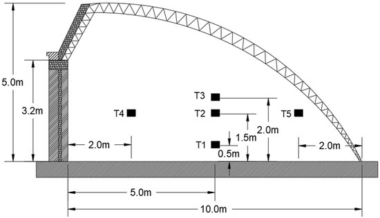
Figure 4.
Side view of the inner measuring point of CSG.
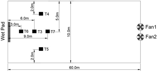
Figure 5.
Top view of the interior measuring point arrangement in CSG.
2.3. Machine Learning Algorithms, Deep Learning Models, and Training Process
Five prediction models were employed in the current paper to analyze greenhouse environmental data. Among these, TCN, GRU, and LSTM are deep learning models, whereas ARMA and ARIMA represent traditional statistical approaches. These models are primarily utilized for time series forecasting, allowing for the prediction of temporal changes in environmental variables such as temperature and humidity. To determine the most effective model, two evaluation metrics were adopted: root mean square error (RMSE) and coefficient of determination (R2). A lower RMSE indicates predictions that are closer to the actual values, while a higher R2 suggests that the model accounts for a greater proportion of variability in the data [26,27,28,29,34,35]. In addition to these metrics, the performance of each model on both the training and testing datasets was examined. By comparing the predicted values with the observed measurements, the most reliable model could be identified. The objective was to select the model that not only fits the training data well, but also maintains accuracy when applied to new, unseen data.
2.3.1. ARMA Method
ARMA is a statistical model used for analyzing and forecasting stationary time series. It combines Autoregressive (AR) and Moving Average (MA) components to capture temporal patterns. The mathematical representation of the ARMA(p, q) model is as follows:
where the AR(p) part uses past values to model long-term dependencies, while the MA(q) part incorporates past error terms to account for short-term fluctuations. Orders and are typically determined by via autocorrelation (ACF) and partial autocorrelation (PACF) functions. ARMA demonstrates strengths in simplicity, interpretability, and computational efficiency when working with small datasets, which has led to its widespread adoption in short-term forecasting across fields such as finance (e.g., stock prices), economics (e.g., inflation), and business (e.g., demand) [20]. However, the model requires stationary input data and performs poorly in capturing nonlinear patterns or complex trends, thereby restricting its applicability to relatively simple time series scenarios [20,21,22,23].
2.3.2. ARIMA Method
ARIMA is a statistical model designed for forecasting non-stationary time series. It extends the ARMA model by incorporating an “integration” component to address non-stationarity. The model is denoted as ARIMA, where represents the order of the autoregressive component, which uses past values to capture long-term dependencies. indicates the degree of differencing applied to transform non-stationary data into stationary form, thereby addressing trends or seasonality.
denotes the order of the moving average component, which incorporates past error terms to model short-term fluctuations. ARIMA is widely used in short-term forecasting tasks such as energy consumption prediction and meteorological data extrapolation [24,35]. Its advantages include adaptability to data with mild trends, a straightforward mathematical formulation that supports theoretical analysis, and relatively low computational requirements, making it suitable for real-time forecasting [25,26,35].
2.3.3. LSTM Method
LSTM is a variant of recurrent neural networks (RNNs) specifically designed to overcome the vanishing gradient problem commonly encountered in traditional RNN architectures. By employing a set of gated units—including input, forget, and output gates—LSTM regulates the flow of information through its memory cells, thereby enabling the effective capture and retention of long-term temporal dependencies in sequential data. This architecture demonstrates superior performance in modeling time series data with complex long-range dependencies [23,24,25,26,27]. Nevertheless, compared to simpler models, LSTM entails higher computational costs and may be prone to overfitting when trained on limited datasets [23,26].
2.3.4. TCN Method
A Temporal Convolutional Network (TCN) is a deep learning architecture specifically designed for modeling sequential and time series data. Built upon the foundation of Convolutional Neural Networks (CNNs), TCNs utilize dilated causal convolutions to effectively capture long-range temporal dependencies while preserving computational efficiency through parallel processing. In contrast to recurrent architectures such as long short-term memory (LSTM) networks, TCNs process input sequences in parallel using a fully convolutional framework, thereby avoiding issues like vanishing gradients and enabling more efficient training on long sequences [20,23]. The architecture introduces several key innovations: dilated convolutions that exponentially expand the receptive field, causal convolutions that preserve temporal order, and residual connections that facilitate stable training of deep networks. These characteristics allow for TCNs to effectively model complex temporal dynamics, accommodate variable-length sequences, and perform well in applications requiring precise temporal understanding [23].
2.3.5. GRU Method
GRU is a simplified variant of RNN, derived from the LSTM architecture. It simplifies the gating mechanism by merging the input and forget gates into a single update gate, while preserving the reset gate [29,30,31,32,33,34]. This structural simplification reduces both the number of parameters and computational complexity compared to LSTM. The GRU effectively captures long-term dependencies in sequential data by regulating the flow of information through its two gating mechanisms: the reset gate controls how much past information to discard, while the update gate determines how much new information to retain [31,34]. This dynamic enables the model to efficiently manage temporal patterns and facilitates faster training due to its streamlined architecture [30,32,33,34].
2.4. Hyperparameter Tuning with K-Fold Cross-Validation
K-fold cross-validation is a robust data partitioning technique used to impartially evaluate the predictive performance of forecasting methods [19,20,21,22,23,24,25,26,27,28,29,30,31,32,33,34,35]. In this approach, the dataset is divided into k mutually exclusive subsets. During each iteration, one subset is used as the validation set, while the remaining k−1 subsets are used for training. The process is repeated k times, with each subset serving exactly once as the validation set. Finally, the performance metrics obtained from the k iterations are averaged to produce a single, comprehensive evaluation score. In this study, a 5-fold cross-validation setup was employed. Hyperparameter tuning was conducted automatically using grid search.
In this study, hyperparameter tuning was conducted automatically using grid search combined with a 5-fold cross-validation setup to ensure the reliability and generalizability of optimal parameters. Detailed tuning processes for each algorithm are as follows:
ARMA: Tuned hyperparameters include autoregressive order and moving average order , with value ranges and (determined via ACF/PACF analysis). The optimal combination was selected by maximizing the validation set R2.
ARIMA: Tuned hyperparameters include autoregressive order , differencing order , and moving average order , with value ranges and , (justified by unit root tests for non-stationarity), and . The optimal combination was chosen by minimizing the validation set RMSE.
LSTM: Tuned hyperparameters focus on the number of neurons per layer, with the following ranges: 1st layer [128, 256, 512], 2nd layer [64, 128, 256], and 3rd layer [32, 64, 128]. The optimal configuration (256, 128, 64) was determined via a grid search combined with an early-stopping strategy (patience = 20) monitoring validation loss. The learning rate uses the default value of the Adam optimizer (0.001).
TCN: Tuned hyperparameters include kernel size [3, 5, 7], dilation rate sequences ([(1, 2, 4, 8), (1, 2, 4, 8, 16)]), and dropout rate ([0.2, 0.3]). The optimal combination (kernel size = 3, dilation rates = (1, 2, 4, 8), dropout rate = 0.2) was selected by prioritizing validation set R2 and training efficiency. The learning rate uses the default value of the Adam optimizer (0.001).
GRU: Tuned hyperparameters focus on the number of neurons per layer, with the following ranges: 1st layer [128, 256, 512], 2nd layer [64, 128, 256], and 3rd layer [32, 64, 128]. The optimal configuration (256, 128, 64) was determined via grid search combined with an early-stopping strategy (patience = 20) monitoring validation loss. The learning rate uses the default value of the Adam optimizer (0.001).
2.5. Data Processing and Partitioning
The raw data, including temperature, humidity, and wind speed collected from the CSG equipped with a PFC system, were first preprocessed to ensure quality and consistency. Missing values were removed to avoid bias in model training, and all features and target variables were normalized to the range [0, 1] using ‘MinMaxScaler’ to unify data scales, facilitating stable model convergence. For time series construction, a sliding window approach with a time step of 40 was adopted to convert the raw data into input–output pairs. Specifically, each input sequence (X) consisted of 40 consecutive time steps of multi-feature data, and the corresponding output (y) was the target variable at the next time step, preserving the temporal dependencies inherent in the greenhouse microclimate data. The dataset was partitioned into training and testing sets using an 8:2 ratio, following temporal continuity. The first 80% of the samples were assigned to the training set and the remaining 20% to the testing set, with no random shuffling to maintain the integrity of the time series structure. Detailed sample sizes for each subset are as follows:
- –
- Temperature data (720 measurements per point): 576 training samples and 144 testing samples.
- –
- Humidity data (300 measurements): 240 training samples and 60 testing samples.
- –
- Wind speed data (180 measurements): 144 training samples and 36 testing samples.
For model validation, an early-stopping strategy was implemented to prevent overfitting. During training, the testing set was temporarily used as the validation set to monitor the validation loss (‘val_loss’). Training was terminated if no improvement in validation loss was observed for 20 consecutive epochs, and the model weights corresponding to the minimum validation loss were restored to ensure optimal generalization performance. All data processing and partitioning steps were executed in the Jupyter Notebook 6.5.4. environment.
2.6. Model Construction and Training
2.6.1. Machine Learning Models
The implementation of the ARMA model involves loading temperature data from Excel files, screening out feature columns and target columns, removing missing values to ensure data integrity, and normalizing data to [0, 1] range using MinMaxScaler for consistent scaling. The model is constructed using the create_arma_dataset function using a univariate approach, utilizing only historical data from the target sequence as input (without integrating multiple features since ARMA is a univariate model). A time step length of 40 is set to extract target sequence data, generating sequences for training and prediction. The target sequence is divided into training and test sets in an 8:2 ratio while maintaining temporal continuity to meet time series prediction requirements. The model order () is determined using the Autocorrelation Function (ACF) and Partial Autocorrelation Function (PACF) plots (e.g., ). The ARIMA model in the statsmodels library is employed (with d = 0 to simulate ARMA) using training sequences as input. The model fits the training data, generates model summaries to verify parameter estimation and significance, then performs in-sample predictions on the training set and out-of-sample predictions on the test set (with prediction length matching the test set). Finally, the inverse scaling function is applied to normalize both the predicted and actual values, restoring the original temperature scale. Model performance is quantified using root mean square error (RMSE), coefficient of determination (R2), mean square error (MSE), and mean absolute error (MAE). Visualization methods include loss curves, prediction comparison plots, R2 scatter plots, and full-sequence overlay diagrams. While ARIMA and ARMA share core processes—including data loading, preprocessing, univariate series construction, 8:2 time series partitioning, prediction and normalization, and evaluation metrics—the key distinction lies in ARIMA’s introduction of the difference parameter (set to 1 in this study via order = ()). This enables ARIMA to transform non-stationary data into stationary sequences, addressing trend or seasonal issues, whereas ARMA requires stationary data () and relies solely on autoregressive (AR) terms () and moving average (MA) terms () to capture temporal patterns, failing to overcome these limitations.
2.6.2. Deep Learning Models
This study selects three common deep learning models—GRU, LSTM, and TCN—for time series prediction in greenhouse environments. In data processing, all three models follow the same workflow: reading temperature data from Excel files, filtering out feature columns and target columns, removing missing values, and then normalizing the data to [0, 1] range using MinMaxScaler. Training samples are constructed using 40 time steps of sliding windows, each containing multi-dimensional environmental feature data from consecutive time steps and the predicted target value for the next moment. After partitioning the time series at an 8:2 ratio, the data dimensions are uniformly adjusted to [samples, time steps, features] to meet model input requirements. In model construction, GRU adopts a three-layer structure (neural units: 256,128,64), with the first two layers retaining sequence information (return_sequences set to True) and outputting single-value predictions through a fully connected layer. Its distinctive characteristic is that it combines the forget gate and input gate into an update gate mechanism, which leads to a reduced parameter scale. Similarly, LSTM also has a three-layer structure (neural units: 256,128,64), with the first two layers similarly set to return_sequences True. It handles sequence information through independent forget gate, input gate, and output gate mechanisms, making it better suited for capturing complex temporal dependencies, although its parameter scale exceeds that of GRU. TCN constructs multi-scale receptive fields through causal convolution (padding = ‘causal’) with dilation rates (1, 2, 4, 8), employing a custom TCNLayer stack architecture that demonstrates superior performance in high-frequency feature extraction. During training, all three models utilize MSE loss with Adam optimization, set to a batch size of 32 and a maximum iteration count of 1500. The early stopping strategy for GRU and LSTM allows for the tolerance of up to 20 epochs of loss stagnation, while TCN maintains this threshold at 10 epochs. Predictions are normalized through inverse scaling and are evaluated using RMSE, R2 metrics, and visualizations. Practical applications reveal GRU’s distinct advantages in greenhouse environmental time series prediction: its compact parameter architecture reduces training time while maintaining comparable accuracy to LSTM, enhancing computational efficiency. Compared to TCN’s complex network structure, GRU’s simpler design requires fewer computing resources and is more deployable, making it better suited for precision control scenarios in greenhouse environments where practicality and efficiency are paramount.
3. Results
3.1. Temperature Distribution
Air temperature results were collected from seven locations (T1–T7) every 30 min over four days: 23–26 August. Figure 6 is plotted with the x-axis representing the time period from 23 August to 26 August and the y-axis indicating temperature in degrees Celsius. Each of the seven curves corresponded to a specific measurement point. Key time markers are included in the figure, such as the system start time at 9:00 AM. During this period, the PFC system was in operation, which led to noticeable daily fluctuations and spatial differences in air temperature. All monitoring points exhibited similar temperature trends. The lowest temperatures were observed between 4:00 AM and 6:00 AM, ranging from 20.1 °C to 24.2 °C. The peak temperatures occurred between 9:00 AM and 9:30 AM. For example, on 24 August, the temperature at monitoring point T3 reached 64.0 °C, which corresponded to the period of the highest temperature at this monitoring point on that day. The cooling system was activated at 09:00 AM and entered a stable cooling state at 10:00 AM; within 30 min after reaching stable operation, the temperature decreased by 10–20 °C. On 23 August, the temperature at measurement point T3 dropped from 55.2 °C at 9:30 AM to 45.5 °C at 10:00 AM. This rapid temperature reduction indicates that the PFC system produced an immediate and effective cooling response. A secondary temperature increase was observed between 5:00 PM and 6:00 PM. For instance, on 23 August, the temperature at measurement point T7 rose from 31.1 °C at 4:30 PM to 36.5 °C at 5:00 PM. This increase may have resulted from heat accumulation following the closure of the thermal insulation curtain. Significant spatial variations were evident in the temperature distribution across the monitored points. Among them, point T3 recorded the highest average temperature of 38.7 °C, whereas point T6 was the coolest, with an average temperature of 30.2 °C. This suggests that the cooling effect was not uniformly distributed throughout the greenhouse. Locations closer to the wet pad, such as T2, were consistently 2–5 °C cooler than areas near the rear wall, such as T4—particularly between 10:00 AM and 3:00 PM. Although the actual cooling effects—reflected in temperature drops, humidity increases, and elevated air velocity—began around 10:00 AM, labeling the start time as 9:00 AM allows for a clearer comparison of environmental conditions before and after the PFC system activation.
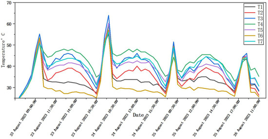
Figure 6.
Air temperature across seven monitoring points.
3.2. Humidity Distribution
Relative humidity was measured at five locations (T1–T3, T6–T7) while the PFC system was in operation from 09:00 to 16:00 between 23 and 26 August. Figure 7 presents the changes in humidity over time. The x-axis spans from 09:00 to 17:00, while the y-axis represents relative humidity in percentage. Each of the five curves corresponds to a measurement point (T1–T3, T6–T7), allowing for a direct comparison of humidity variations across different locations within the greenhouse. The data illustrates the variation in humidity caused by evaporative cooling. Humidity levels ranged from 33% to 80%. Point T6, located nearest to the wet pad, recorded the highest average humidity of 68.5%. The other points followed in descending order: T2 at 56.3%, T1 at 55.7%, T3 at 50.1%, and T7 at 48.9%. This distribution aligns with the anticipated airflow direction—from the wet pad toward the exhaust fans—demonstrating the system’s influence on humidity distribution within the greenhouse. During the daytime, humidity exhibited a clear trend: from 09:00 to 12:00, it generally decreased. On 24 August, for instance, the humidity at T6 increased from 65% at 12:00 to 79% at 16:00. This increase corresponded with the enhanced evaporative cooling effects as the system continued to operate. Once the system was turned off, humidity levels dropped rapidly. For example, on 23 August, the humidity at T6 fell from 78% at 16:30 to 46% at 17:00. This sharp decline illustrated the significant role of the PFC system in maintaining high humidity levels. The figure reveals both consistent daily trends and spatial differences in humidity levels. All measurement points exhibited an initial decline followed by an increase in humidity. Notably, T6 consistently recorded the highest humidity, which confirms its location in the coolest and most moisture-retentive area of the greenhouse.
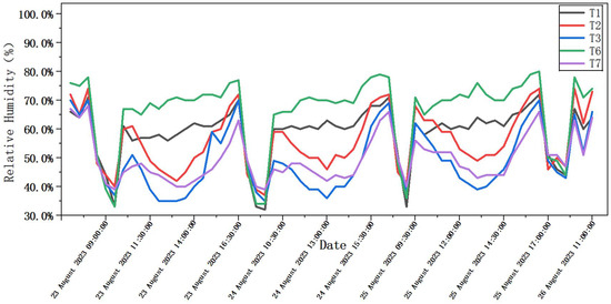
Figure 7.
Temporal variations in humidity across multiple monitoring points.
3.3. Airflow Velocity Characteristics
Airflow velocity was measured at three points (T2, T6, and T7) during the cooling system’s operation to better understand the airflow patterns created by the PFC system, as shown in Figure 8. illustrated the variation in airspeed over time, with time plotted on the x-axis (from 09:00 to 17:00) and wind speed (in m/s) on the y-axis. The three curves represent the three measurement points. The figure reveals that T6 exhibited more rapid increases in airspeed upon system activation and quicker decreases after shutdown, which reflects the immediate influence of the wet pad system. Smaller fluctuations in the T6 curve during midday suggest minor adjustments in fan operation. As shown in the figure, there is a strong correlation between high wind speeds (≥2.0 m/s) and significant temperature drops (≥6 °C). In contrast, this correlation is weaker under low-wind-speed conditions. These observations suggest that, in areas further from the wet curtain (e.g., T7), improvements in airflow distribution may be necessary to achieve a more uniform microclimate within the greenhouse. Point T6, located 3 m from the wet pad, recorded the highest average airspeed of 2.31 m/s. In comparison, Point T2, situated 6 m away from the wet pad, had an average airspeed of 1.58 m/s. Point T7, which was the furthest from the pad at 9 m, exhibited the lowest average airspeed of 0.67 m/s. This observed decline in airspeed with increasing distance from the wet pad aligns with the expected performance of negative-pressure ventilation systems. Examining changes over time, peak airspeeds were observed between 15:00 and 16:30. For example, on 23 August, T6 reached 2.42 m/s at 15:30, a time that coincided with the highest afternoon temperatures. At system startup, wind speed rapidly increased from near-zero to between 1.8 and 2.4 m/s from 09:00 to 10:00, and remained relatively stable until approximately 16:30. After system shutdown, airspeed declined sharply, dropping below 0.1 m/s within 30 min. On 23 August, for instance, T2 decreased from 2.21 m/s at 16:30 to only 0.04 m/s at 17:00. Higher airspeeds at T6 were associated with more pronounced cooling and humidification effects. Compared to T7, T6 experienced temperature reductions of 5–8 °C and humidity increases of 10–15%. These results indicate that increased airflow has a direct impact on the greenhouse microclimate.
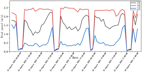
Figure 8.
Temporal evolution of wind speed at three monitoring points.
4. Discussion
4.1. Correlation Analysis
Pearson correlation coefficients are computed and visualized with a heatmap (Figure 9), revealing a strong negative correlation between temperature, humidity, and wind speed [23,30]. Temporally, data are collected at 30 min intervals, capturing the complete process from PFC system start-up to shutdown. Spatially, the setup includes seven temperature monitoring points, five humidity monitoring points, and three wind speed monitoring points, strategically distributed across different zones of the greenhouse. These collectively constitute a microclimate variable dataset, providing ample samples for correlation analysis [30]. Specifically, at monitoring points close to the wet pad, such as T6, increased wind speed significantly enhances air circulation and heat dissipation. On average, each 0.5 m/s rise in wind speed results in a 3.2 °C decrease in temperature, with the correlation coefficient reaching −0.82. At distant points such as T7, the correlation coefficient decreases to −0.51, which can be attributed to airflow attenuation and heat accumulation. This observation reflects a “distance−correlation intensity” attenuation pattern [28,29]. Humidity and wind speed exhibit a positive correlation. In regions influenced by the wet pad, such as T6, high-speed airflow enhances the evaporative humidification effect, resulting in a correlation coefficient of 0.75 between wind speed and humidity. However, as distance increases, for instance at T7, airflow diffusion reduces the efficiency of evaporation. Consequently, the correlation coefficient declines to 0.32, and humidity becomes more dependent on ambient temperature. A spatial correlation in temperature gradients is also evident. Along the airflow path from the wet pad to the fan, temperature demonstrates a linear increasing trend. The average temperatures at T6 (3 m from the wet pad), T2 (6 m from the wet pad), and T7 (9 m from the wet pad) rise sequentially by 2.3 °C and 5.8 °C. There is a positive correlation with distance, with a coefficient of 0.89. In the vertical direction from 0.5 m to 2.0 m, the temperature difference is notable. The correlation coefficient between T1 and T3 is 0.68, indicating that the plant canopy height of 1.5 m serves as a critical layer for temperature regulation. Hence, the temperature input variables are T3, T4, and T5, with output variables being T1, T2, T6, and T7. The humidity input variables are T2, T3, and T6, and output variables are T1 and T7. The wind speed input variables are T6 and T7, and the output variable is T2.
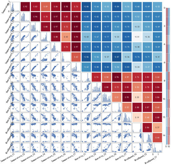
Figure 9.
Visualization of multivariate correlation analysis for greenhouse microclimate.
4.2. Time Series Prediction via ARMA Model
The R2 of ARMA in different factors is shown in Figure 10. For temperature prediction, the training set R2 reaches 0.990; however, the test set R2 drops sharply to −1.800 due to nonlinear disturbances caused by intense solar radiation at noon. Additionally, the model fails to adapt to abrupt temperature changes associated with the activation and deactivation of wet curtains. For humidity prediction, the training set R2 is 0.949, but the test set R2 decreases to −0.438, largely affected by the nonlinearity of evaporation processes. The model also struggles to capture the dynamic relationship between wind speed and humidity in wet-curtain influence zones, such as T6. Regarding wind speed prediction, the training set R2 is 0.777, whereas the test set R2 is only −0.320, primarily due to spatial heterogeneity in airflow attenuation. The model is unable to accurately describe the coupling mechanisms between wind speed, temperature, and humidity. Complete sequence comparison figures reflect overlay deviations between full-period original data and prediction results, as shown in Figure 11. The simulation results of the test set exhibit a complete divergence from the experimental test results. In summary, the ARMA model is based on the assumption of linear stationarity, which limits its applicability to short-term steady-state predictions of microclimate parameters. In scenarios involving nonlinear interactions between temperature and wind speed or dynamic fluctuations in humidity due to evaporation, the model’s performance, as indicated by the R2 value, deteriorates significantly. This underscores the model’s limitations in capturing the complexities of microclimate systems characterized by nonlinear and dynamic behavior.
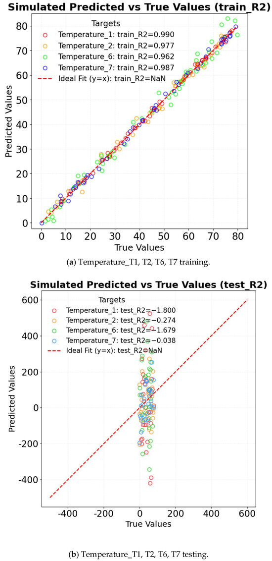
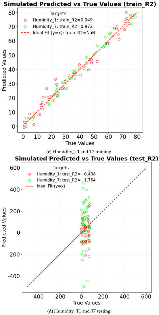
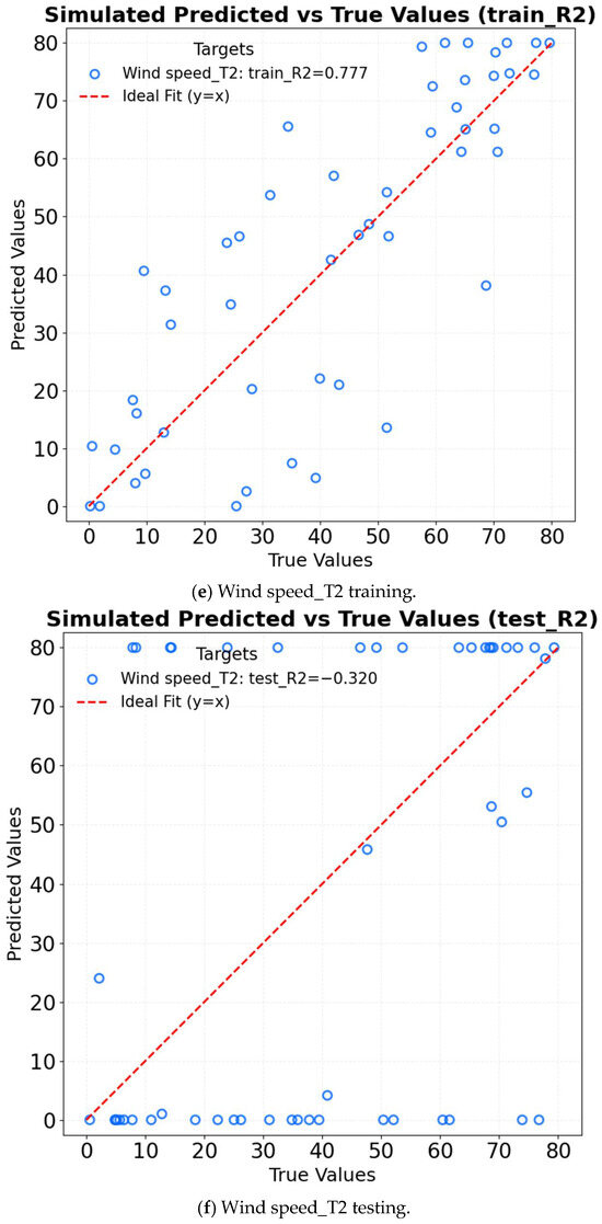
Figure 10.
R2 of ARMA in different factors.
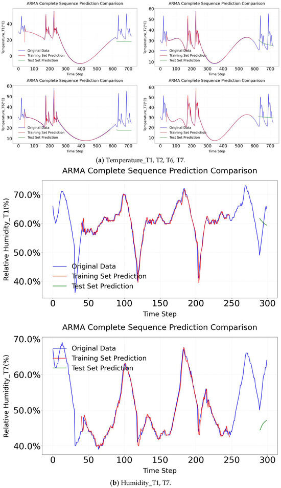
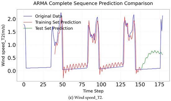
Figure 11.
ARMA complete sequence comparison.
4.3. Time Series Prediction via ARIMA Model
The R2 of ARIMA in different factors is shown in Figure 12. For temperature prediction, the model achieves an R2 of 0.977 on the training set; however, the R2 drops significantly to −1.704 on the test set. This indicates that the model fails to capture sudden temperature fluctuations caused by wet pads. In the case of humidity prediction, the training set R2 is 0.879, while the test set R2 is −0.124, suggesting that the model cannot adequately capture the nonlinear relationship between evaporation and humidity. Regarding wind speed prediction, the training set R2 is 0.749, but the test set R2 decreases to −0.164, indicating that the model struggles to account for spatial variations in airflow attenuation. Complete sequence comparison figures reflect overlay deviations between full-period original data and prediction results, as shown in Figure 13. ARIMA also fails in complex microclimates.
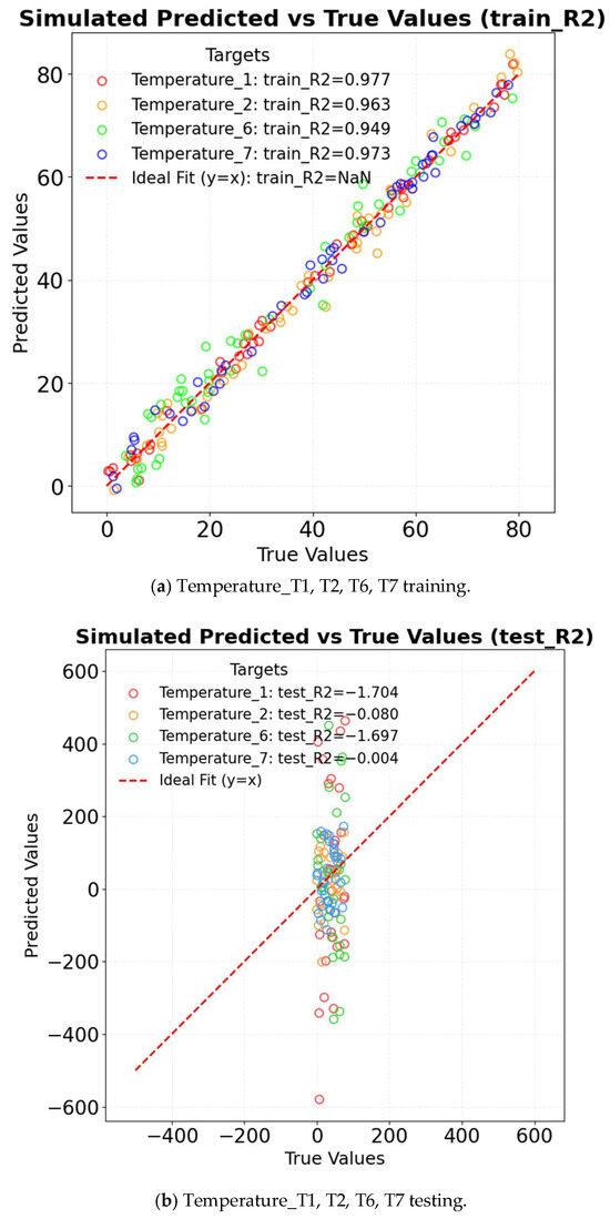
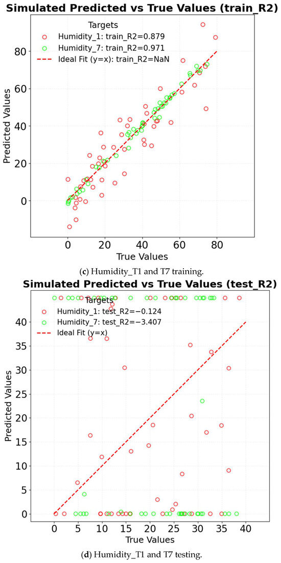
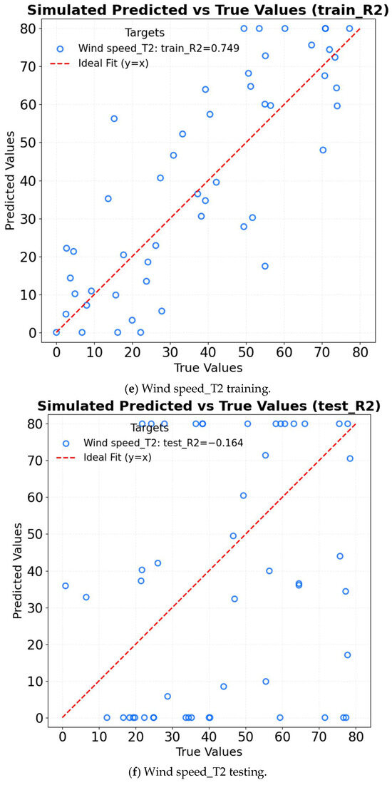
Figure 12.
R2 of ARIMA in different factors.
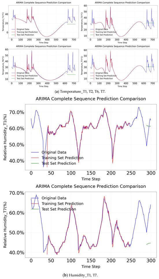
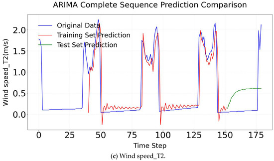
Figure 13.
ARIMA complete sequence comparison.
4.4. Time Series Prediction via LSTM Model
Long short-term memory (LSTM) employs gating mechanisms to effectively capture long-term dependencies in time series data, making it particularly suitable for predicting greenhouse microclimate parameters such as temperature, humidity, and wind speed. Compared to traditional models like ARMA and ARIMA, LSTM demonstrates superior performance in handling nonlinear correlations. Additionally, it supports multi-feature inputs—such as the combined effects of T3, T4, and T5—enabling the model to capture complex interactions among variables efficiently. In the data preprocessing stage, datasets are first loaded, followed by the selection of target variables (T1, T2, T6, T7) and relevant features. Missing values are removed to ensure data integrity, and the data is subsequently normalized to the [0, 1] range using MinMaxScaler. A sliding window approach is applied to construct time series datasets, with a time step of 40 to align with the 30 min sampling intervals. The input sequences consist of 40 time steps with multiple features, while the target corresponds to the core measurement at the 41st time step. The model architecture comprises three LSTM layers containing 256, 128, and 64 neurons, respectively, followed by a fully connected output layer. The gating units within each LSTM layer selectively retain critical temporal information. The model is trained using mean squared error (MSE) as the loss function and the Adam optimizer. To prevent overfitting, an early stopping strategy with a patience value of 20 epochs is implemented. The dataset is partitioned into training and testing sets at an 8:2 ratio. Finally, prediction results are denormalized to their original physical scales: temperature in degrees Celsius (°C), humidity in percentage (%), and wind speed in meters per second (m/s). Model performance is evaluated using root mean squared error (RMSE), coefficient of determination (R2), and mean squared error (MSE). The R2 of LSTM in different factors is shown in Figure 14. For temperature prediction, the model achieves an R2 of 0.985 on the training set and 0.918 on the test set, demonstrating superior performance compared to ARIMA in capturing abrupt temperature fluctuations caused by wet curtains. In the case of humidity prediction, the training set yields an R2 of 0.972, while the test set achieves an R2 of 0.896, indicating the model’s effectiveness in capturing the nonlinear relationship between evaporation and wind speed. Regarding wind speed prediction, the model attains an R2 of 0.965 on the training set and 0.849 on the test set, showing strong adaptability to spatial variations in airflow attenuation. The LSTM model’s capability to capture both long-term and short-term trends is illustrated in Figure 15. The strength of the LSTM lies in its ability to balance long-term dependencies with computational efficiency through its gating mechanisms [27]. Consequently, its overall performance surpasses that of traditional linear models.
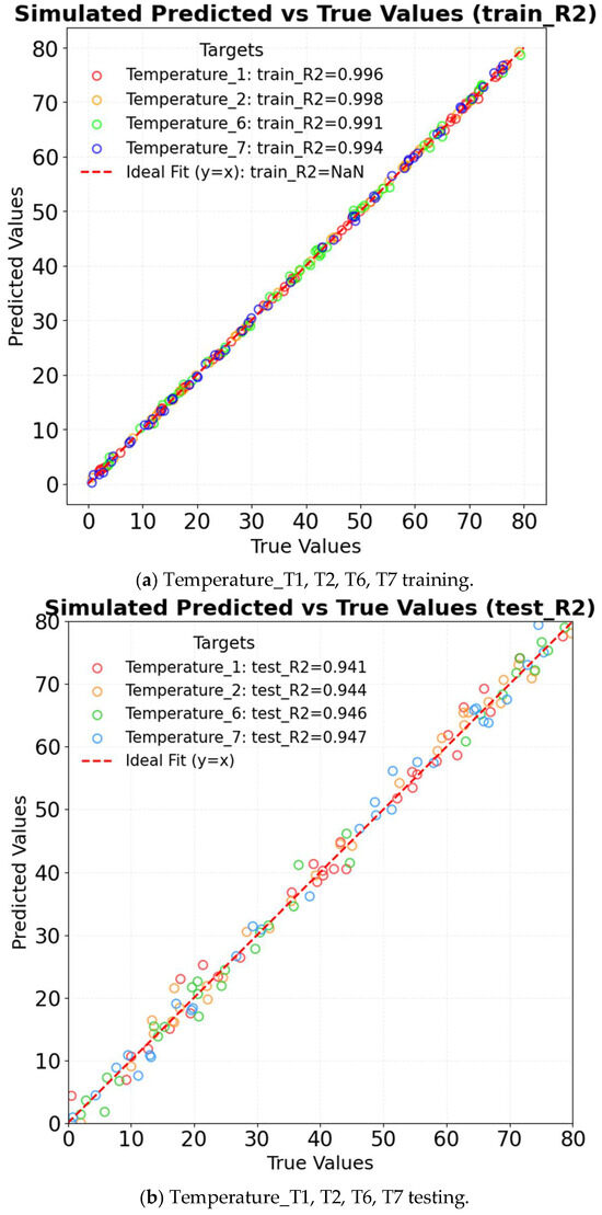
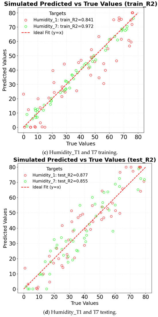
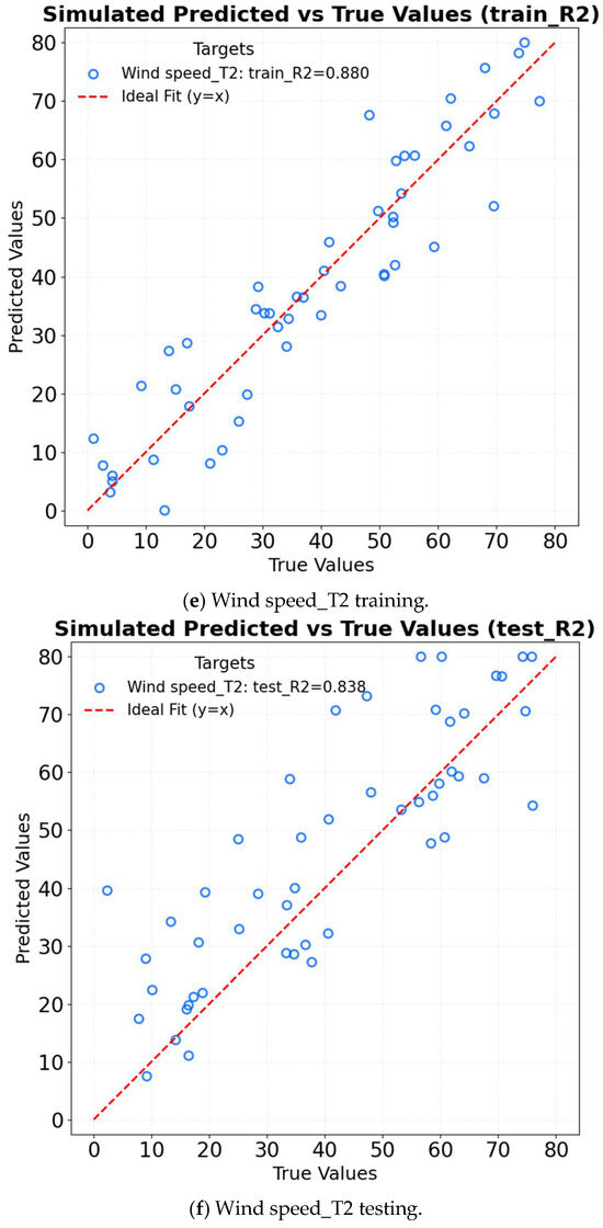
Figure 14.
R2 of LSTM in different factors.
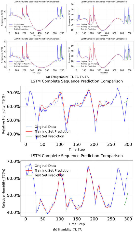
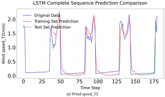
Figure 15.
LSTM complete sequence comparison.
4.5. Time Series Prediction via TCN Model
TCN is specifically designed to predict key greenhouse microclimate parameters, such as temperature, humidity, and wind speed. By utilizing dilated convolutions, it effectively captures multi-scale temporal dependencies, thereby addressing the limitations of traditional linear models like ARMA and ARIMA in modeling nonlinear patterns and long-range temporal correlations [23]. The R2 of TCN in different factors is shown in Figure 16. In temperature prediction (T1–T7), the TCN exhibits strong performance, with notable results in key metrics. Specifically, Temperature_T6 yields a training set R2 of 0.984 and a test set R2 of 0.909, while Temperature_T7 yields a training set R2 of 0.989 and a test set R2 of 0.961. These values indicate that the model has a robust capability in modeling temperature dynamics, including the effective capture of changes caused by wet curtains. In humidity prediction (Humidity_T1, Humidity_T7), despite indications of improved accuracy in capturing the nonlinearity between evaporation and wind speed, the model yields extremely low R2 values (e.g., Humidity_T7 test set R2 = 0.100), suggesting inadequate model fitting. For wind speed prediction (Wind speed_T2), the results are relatively promising (test set R2 = 0.837). The TCN model’s result comparison is shown in Figure 17. The comparison results of all training sets are excellent. However, the testing results set do not correspond to the experimental result.
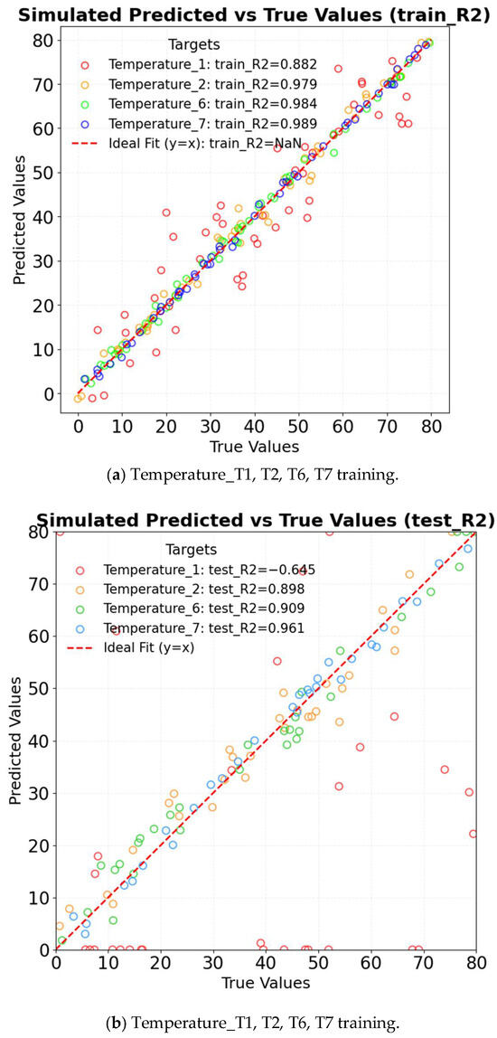
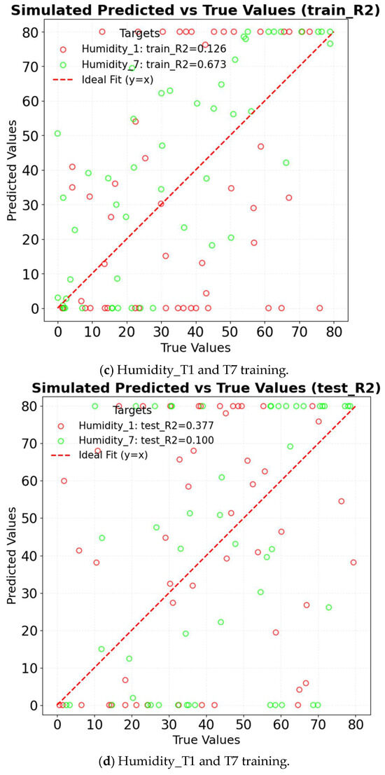
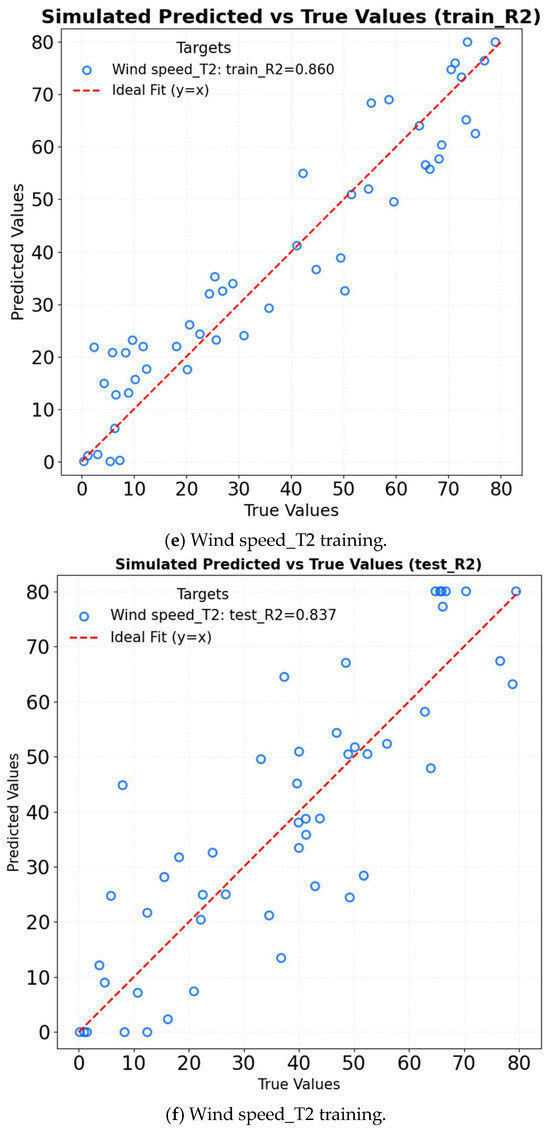
Figure 16.
R2 of TCN in different factors.
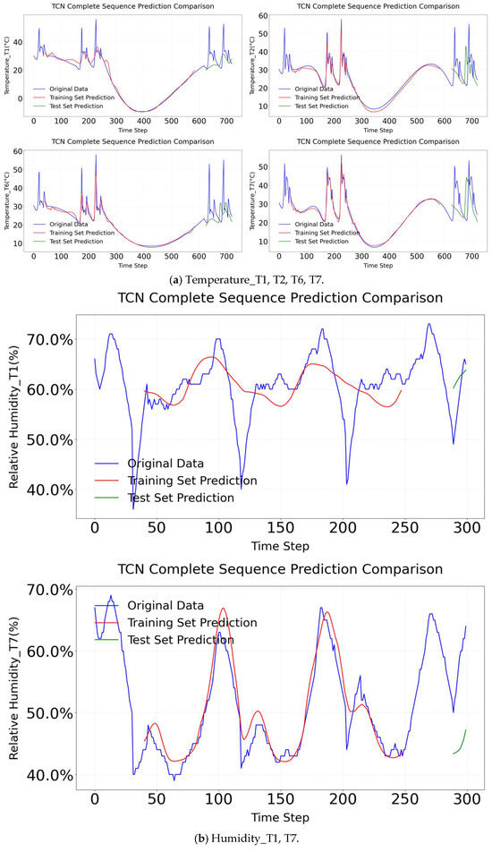
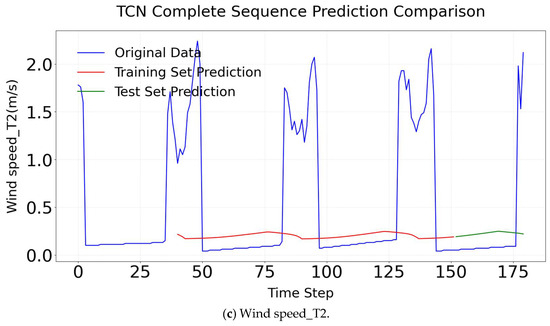
Figure 17.
TCN complete sequence comparison.
4.6. Time Series Prediction via GRU Model
GRU simplifies the gating mechanism of LSTM networks while still effectively capturing long-term temporal dependencies [29,30,31]. This structural simplification enhances computational efficiency and reduces complexity, making GRU particularly suitable for predicting greenhouse microclimate parameters such as temperature, humidity, and wind speed. Compared to LSTM, GRU merges the update and reset gates, thereby eliminating redundant parameters and accelerating training convergence without compromising prediction accuracy [30]. In contrast to TCNs, GRU avoids the computational burden associated with stacked dilated convolutions [29]. As a result, GRU achieves a more favorable balance between efficiency and performance when modeling moderately complex nonlinear relationships. The R2 of GRU in different factors is shown in Figure 18. For temperature prediction, the model achieves an R2 of 0.997 on the training set and 0.955 on the test set. It captures the sudden temperature changes caused by wet curtains more effectively than LSTM. Its predictive accuracy is comparable to TCN, while convergence is achieved 30% faster. In humidity prediction, the model attains an R2 of 0.936 on the training set and 0.973 on the test set. It accurately captures the nonlinear relationship between evaporation and wind speed, performing on par with TCN. Additionally, it reduces training time by 30% compared to LSTM. Regarding wind speed prediction, the model demonstrates R2 values of 0.776 on the training set and 0.546 on the test set. GRU adapts more effectively to spatial attenuation than LSTM and exhibits superior efficiency to TCN when processing large datasets. The GRU model’s result comparison is shown in Figure 19. The comparison results of all training sets and testing results set are all excellent.
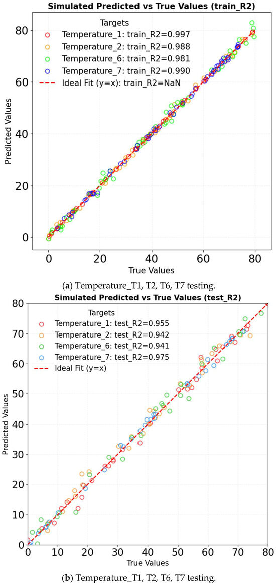
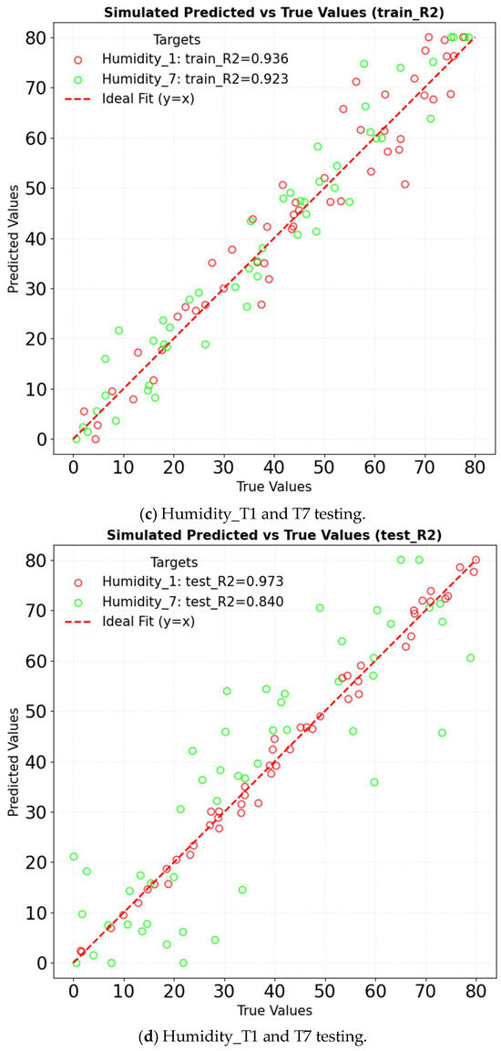
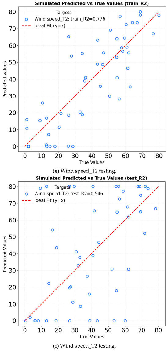
Figure 18.
R2 of GRU in different factors.
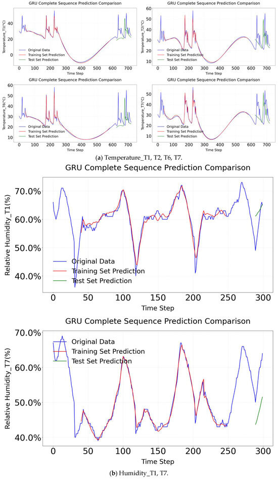
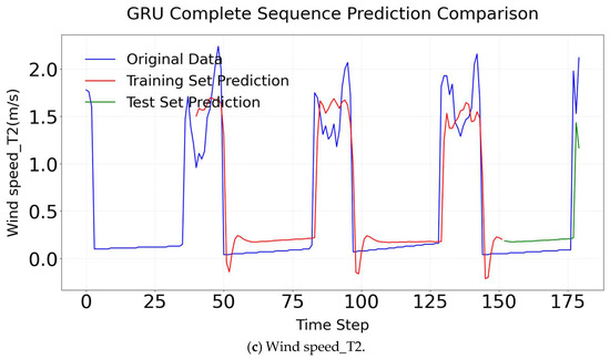
Figure 19.
GRU complete sequence comparison.
4.7. Performance Analysis of Five Models in Greenhouse Microclimate Prediction
ARMA, ARIMA, LSTM, TCN, and GRU exhibit different performance levels in predicting greenhouse temperature, humidity, and wind speed, as illustrated in Figure 20, Figure 21 and Figure 22. In terms of humidity prediction at monitoring point T1, GRU demonstrates a clear advantage. Its RMSE is only 0.013, the R2 value reaches 0.946, and the MSE is 0.0. At the T7 monitoring point, although LSTM performs best, GRU achieves nearly comparable results, with an RMSE of 0.02 and an R2 of 0.924. For wind speed prediction at the T2 measurement point, LSTM is the top performer. However, GRU, with an RMSE of 0.354 and an R2 of 0.762, outperforms both ARMA and ARIMA. Although a performance gap exists between GRU and LSTM, it is relatively small. In terms of temperature prediction across multiple monitoring points, GRU demonstrates superior performance at several locations. At the T1 point, GRU achieves an R2 of 0.995, surpassing LSTM and other models. At the T2 point, GRU performs comparably to LSTM and better than other models. At the T6 point, GRU achieves the lowest RMSE and the best overall performance. Even at the T7 point, where LSTM has a slight advantage, GRU still achieves an R2 of 0.989, indicating highly accurate predictions. Overall, in predicting greenhouse temperature, humidity, and wind speed, deep learning models such as LSTM, TCN, and GRU outperform traditional models like ARMA and ARIMA. Among these, GRU stands out due to its consistently strong performance across different monitoring points and parameters, demonstrating robust overall capabilities. In addition to its high prediction accuracy, GRU offers structural and training efficiency advantages. By simplifying LSTM’s gating mechanism, GRU reduces the number of model parameters and achieves a training speed that is 30% faster than LSTM. Compared to TCN, GRU is more efficient when processing large datasets. Due to its high computational efficiency, GRU is particularly suitable for greenhouse environment-control systems with limited computing resources. It provides reliable support for the precise control of greenhouse cooling systems and holds significant practical value.
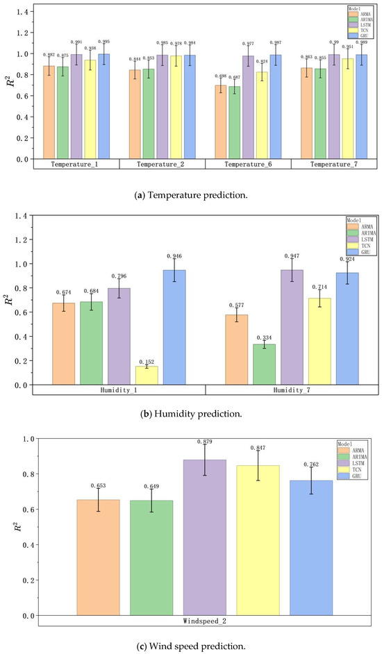
Figure 20.
R2 of different model predictions.
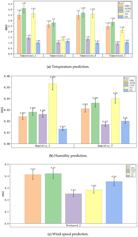
Figure 21.
RMSE of different model predictions.
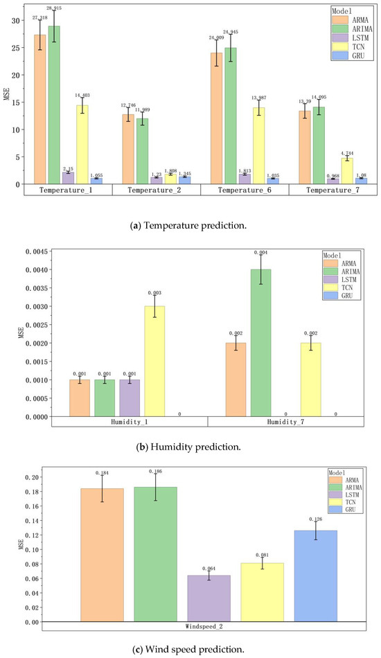
Figure 22.
MSE of different model predictions.
4.8. Comparison with Numerical Methods for Continuous Microclimate Analysis
In the solar greenhouse equipped with a wet-curtain–fan cooling (PFC) system, the machine learning (ML) and deep learning (DL) methods adopted in this study showed significant advantages compared to traditional numerical methods (such as computational fluid dynamics, CFD) in coping with annual weather changes and continuous analysis of the microclimate.
Numerical methods such as CFD are good at simulating complex fluid dynamics and heat and mass transfer mechanisms, but computational fluid dynamics (CFD) simulations need high computational power and thus are resource-hungry [36]. Thus, many practical engineering applications, such as simulations of highly turbulent flows and simulations of large computational domains, becomes very expensive [37]. CFD needs a very fine grid to compute different scenarios at an accepted scale and have a grid-independent solution. The fine-grid requirements step down step size, thus increasing the time for computation; this results in a long problem-solving time for the computer, making it expensive [38]. The ML/DL model in this study leverages historical sensor data and multi-seasonal training (covering varying solar radiation, ambient temperature, and precipitation) to capture the nonlinear relationships between outdoor weather fluctuations and indoor microclimate parameters (temperature, humidity, wind speed) without explicit physical modeling [39]. For instance, the GRU effectively balances long-term dependencies like seasonal trends with short-term fluctuations such as daytime temperature peaks, enabling real-time adaptation to weather changes. With computational costs significantly lower than CFD methods, it achieves continuous, low-latency analysis—a critical capability for dynamic greenhouse management.
The annual weather change will lead to the non-stationarity of microclimate dynamics. The traditional CFD solvers, when dealing with unsteady flows, rely on predefined physical equations, and it is difficult to fully capture this non-stationarity without continuous update of seasonal adjustment parameters for specific sites, which is unrealistic for long-term monitoring. If the number of pressure-correction iterations is insufficient or if the parameters are not adjusted in a timely manner, they are prone to divergence, especially in the case of large-scale meshes or changing flow conditions [40]. However, the ML/DL approach in this study demonstrates strong adaptability. The LSTM and GRU models utilize gating mechanisms to dynamically adapt to changing weather patterns, prioritizing relevant historical data such as temperature–humidity curves from previous seasons. Cross-validation results across five folds confirm that these models maintain stable performance, even when predicting unobserved weather conditions, enabling year-round continuous analysis without requiring manual calibration.
Numerical methods exhibit high spatial accuracy in simulating microclimate gradients, making them valuable for facility design. However, despite decades of advancements in research and engineering practice, computational fluid dynamics (CFD) techniques still encounter significant challenges [41]. Specifically, they are difficult to apply to real-time scenarios when integrating annual weather changes. Although the ML/DL model in this study cannot reproduce the fine spatial details of CFD, it can provide accurate and efficient predictions across seasons at key monitoring points (T1–T7).
In conclusion, ML/DL demonstrates superior advantages through its efficiency, adaptability to weather variations, and practical value in real-time management. While numerical methods remain indispensable for detailed physical modeling and facility design, the model developed in this study provides an economically efficient and scalable solution for year-round monitoring.
5. Conclusions
The variation process of the microclimate environment within solar greenhouses under the influence of PFC systems was systematic investigated using experimental measurements. According to the spatial distribution perspective, the microclimate in greenhouses with PFC systems exhibit significant non-uniformity. The temperature and humidity gradients along the wet-pad–fan direction (T6 → T2 → T7) and vertically (T1 → T2 → T3) differ significantly, and the wind speed also decreases significantly with distance (from 2.31 m/s in T6 to 0.67 m/s in T7). This spatial feature indicates that the influence of airflow distribution should be fully considered when optimizing the model. ARMA, ARIMA, LSTM, TCN, and GRU were used in predicting microclimate parameters (temperature, humidity, and wind speed). The results indicate that deep learning models significantly outperform traditional linear models in capturing the complex nonlinear relationships and spatiotemporal dynamics within greenhouse environments. Furthermore, notable differences in applicability and predictive accuracy were observed among the various models. Specifically, the traditional time series models ARMA and ARIMA demonstrated relatively limited performance in forecasting greenhouse microclimatic conditions.
The ARMA model is based on linear and stationarity assumptions, which are reasonable under short-term stable conditions; however, it is incapable of handling nonlinear fluctuations caused by factors such as wet pad start–stop cycles or solar radiation. The R2 values for temperature, humidity, and wind speed in the test set have dropped significantly, even becoming negative, reflecting the model’s limitations. Although ARIMA addresses non-stationarity through differencing, its linear structure still hampers its ability to capture the highly nonlinear interactions between evaporation and wind speed.
In contrast, deep learning models exhibit excellent performance in handling complex dynamics. LSTM captures long-term dependencies through gating mechanisms, and it outperforms traditional models in tracking sudden temperature changes and spatial airflow attenuation, with R2 values in the test set being 0.941 for temperature, 0.855 for humidity, and 0.879 for wind speed, respectively. TCN shows outstanding performance in identifying high-frequency fluctuations and extreme nonlinear features, especially in wind speed prediction (with an R2 of 0.847). However, it has limitations in modeling certain temperature dynamics (e.g., the R2 of the T1 test set is −0.645) and humidity evaporation processes (e.g., the R2 of the T7 test set is 0.1). GRU achieves a good balance between accuracy and efficiency. It attains the highest prediction accuracy in temperature (test set R2 = 0.975) and humidity (test set R2 = 0.973) prediction, and is only slightly inferior to TCN in wind speed prediction. Notably, GRU converges approximately 30% faster than LSTM and is more efficient than TCN on large-scale datasets, which makes it highly suitable for greenhouse applications with limited computational resources.
This study clarifies the limitations of traditional models: compared to traditional machine learning models (such as multiple regression [12] and support vector machine regression [18]) limited to capturing single parameters or linear relationships, it further quantifies the failure degree (with R2 being negative) of traditional time series models like ARMA and ARIMA in handling nonlinear microclimate fluctuations (e.g., from wet curtain start–stop and solar radiation) and verifies their shortcomings in complex dynamic scenarios through multi-parameter synchronous prediction. It deepens our scenario-based understanding of deep learning models: building on early neural networks [16,20] and recent models like LSTM [26], GRU [29], and RNN−TCN [23], through systematic comparison, it clarifies GRU’s balanced advantages in accuracy (temperature R2 = 0.975) and efficiency (30% faster than LSTM) in greenhouse multi-parameter prediction, reveals TCN’s limitations in specific scenarios, provides more specific model selection guidance, and fills gaps in existing research regarding deep learning models’ adaptability to complex microclimates. It also establishes a cross-model comparison framework: breaking through previous studies’ “single model for single task” limitation [17,19], by using parallel tests of five models, it reveals differences in models’ adaptability to greenhouse microclimates’ spatial non-uniformity, offering comprehensive selection criteria for practical scenarios with limited computing resources or real-time regulation needs, and also addressing early studies’ lack of diverse model application scenarios.
In summary, deep learning models, particularly GRU, offer more reliable methodological support for greenhouse microclimate prediction, thereby facilitating precise regulation of cooling systems and scientifically informed crop management. Future research should aim to expand the number of monitoring points, integrate crop canopy structure information, and explore multi-scale prediction approaches tailored to minute- and hour-level timeframes in order to further enhance the model’s adaptability and practical applicability to complex agricultural environments.
Author Contributions
Conceptualization, W.L. and M.Y. (Mengmeng Yang); methodology, Z.X.; validation, Y.B.; formal analysis, Y.L.; investigation, K.P.; resources, M.Y. (Mingze Yao); data curation, Y.L.; writing—original draft preparation, W.L.; writing—review and editing, M.Y. (Mengmeng Yang); funding acquisition, F.Z. All authors have read and agreed to the published version of the manuscript.
Funding
This research was funded by [Postdoctoral General Project] grant number [2021M693862] and the APC was funded by [Feng Zhang].
Data Availability Statement
The datasets presented in this study are available within the article.
Acknowledgments
The author would like to thank all contributors to this study.
Conflicts of Interest
The authors declare no conflicts of interest.
References
- Tong, G.; Christopher, D.M.; Li, T.; Wang, T. Passive solar energy utilization: A review of cross−section building parameter selection for Chinese solar greenhouses. Renew. Sustain. Energy Rev. 2013, 26, 540–548. [Google Scholar] [CrossRef]
- He, X.; Wang, J.; Guo, S.; Zhang, J.; Wei, B.; Sun, J.; Shu, S. Ventilation optimization of solar greenhouse with removable back walls based on CFD. Comput. Electron. Agric. 2018, 149, 16–25. [Google Scholar] [CrossRef]
- He, M.; Jiang, X.; Wan, X.; Li, Y.; Fan, Q.; Liu, X. Design and Ventilation Optimization of a Mechanized Corridor in a Solar Greenhouse Cluster. Horticulturae 2024, 10, 1240. [Google Scholar] [CrossRef]
- López, A.; Valera, D.L.; Molina-Aiz, F.D.; Peña, A. Sonic anemometry to evaluate airflow characteristics and temperature distribution in empty Mediterranean greenhouses equipped with pad–fan and fog systems. Biosyst. Eng. 2012, 113, 334–350. [Google Scholar] [CrossRef]
- Al-Manthria, I.; Al-Ismailia, A.M.; Kotagamab, H.; Khanc, M.; Jeewanthad, L.H.J. Water, land, and energy use efficiencies and financial evaluation of air conditioner cooled greenhouses based on field experiments. J. Arid. Land 2021, 13, 375–387. [Google Scholar] [CrossRef]
- Nam, S.W.; Kim, Y.S. Greenhouse cooling using air duct and integrated fan and pad system. J. Bio-Environ. Control. 2011, 20, 176–181. [Google Scholar]
- Woon, N.S.; Giacomelli Gene, A.; Sung, K.K.; Sabeh, N. Analysis of temperature gradients in greenhouse equipped with fan and pad system by CFD method. J. Bio-Environ. Control. 2005, 14, 76–82. [Google Scholar]
- Gauthier, C.; Lacroix, M.; Bernier, H. Numerical simulation of soil heat exchanger−storage systems for greenhouses. Sol. Energy 1997, 60, 333–346. [Google Scholar] [CrossRef]
- Yuan, M.; Zhang, Z.; Li, G.; He, X.; Huang, Z.; Li, Z.; Du, H. Multi-Parameter Prediction of Solar Greenhouse Environment Based on Multi-Source Data Fusion and Deep Learning. Agriculture 2024, 14, 1245. [Google Scholar] [CrossRef]
- Yang, L.H.; Huang, B.H.; Hsu, C.Y.; Chen, S.L. Performance analysis of an earth–air heat exchanger integrated into an agricultural irrigation system for a greenhouse environmental temperature−control system. Energy Build. 2019, 202, 109381. [Google Scholar] [CrossRef]
- Joudi, K.A.; Farhan, A.A. A dynamic model and an experimental study for the internal air and soil temperatures in an innovative greenhouse. Energy Convers. Manag. 2015, 91, 76–82. [Google Scholar] [CrossRef]
- JuarezMaldonado, A.; BenavidesMendoza, A.; deAlbaRomenus, K.; MoralesDiaz, A. Estimation of the water requirements of greenhouse tomato crop using multiple regression models. Emir. J. Food Agric. 2014, 26, 885. [Google Scholar] [CrossRef]
- Baptista, F.; Bailey, B.; Meneses, J. Measuring and modelling transpiration versus evapotranspiration of a tomato crop grown on soil in a Mediterranean greenhouse. Acta Hortic. 2005, 1, 313–319. [Google Scholar] [CrossRef]
- Guo, L.; Chen, X.; Yang, S.; Zhou, R.; Liu, S.; Cao, Y. Optimized Design of Irrigation Water-Heating System and Its Effect on Lettuce Cultivation in a Chinese Solar Greenhouse. Plants 2024, 13, 718. [Google Scholar] [CrossRef] [PubMed]
- Taki, M.; Ajabshirchi, Y.; Ranjbar, S.F.; Matloobi, M. Application of Neural Networks and multiple regression models in greenhouse climate estimation. Agric. Eng. Int. CIGR J. 2016, 18, 29–43. [Google Scholar]
- He, F.; Ma, C. Modeling greenhouse air humidity by means of artificial neural network and principal component analysis. Comput. Electron. Agric. 2010, 71, S19–S23. [Google Scholar] [CrossRef]
- Linker, R.; Seginer, I.; Gutman, P. Optimal CO2 control in a greenhouse modeled with neural networks. Comput. Electron. Agric. 1998, 19, 289–310. [Google Scholar] [CrossRef]
- Yang, M.; Zhang, F.; Teramoto, K. Statistical model comparison based on variation parameters for monitoring thermal deformation of workpiece in end-milling. Int. J. Adv. Manuf. Tech. 2023, 128, 5139–5152. [Google Scholar] [CrossRef]
- Sethu, V.; Wu, S. Sequential support vector classifiers and regression. In Proceedings of the International Conference on Soft Computing (SOCO’99), Genoa, Italy, 22–25 August 1999. [Google Scholar]
- Ferreira; Pedro, M.; Faria, E.A.; Ruano, A.E. Neural network models in greenhouse air temperature prediction. Neurocomputing 2002, 43, 51–75. [Google Scholar] [CrossRef]
- Li, L.; Chen, S.W.; Yang, C.F.; Meng, F.J.; Sigrimis, N. Prediction of plant transpiration from environmental parameters and relative leaf area index using the random forest regression algorithm. J. Clean. Prod. 2020, 261, 121136. [Google Scholar] [CrossRef]
- Li, Y.; Zou, C.; Berecibar, M.; Nanini-Maury, E.; Chan, J.C.-W.; Bossche, P.v.D.; Van Mierlo, J.; Omar, N. Random forest regression for online capacity estimation of lithium-ion batteries. Appl. Energy 2018, 232, 197–210. [Google Scholar] [CrossRef]
- Gong, L.; Yu, M.; Jiang, S.; Cutsuridis, V.; Pearson, S. Deep learning based prediction on greenhouse crop yield combined TCN and RNN. Sensors 2021, 21, 4537. [Google Scholar] [CrossRef]
- Graves, A.; Mohamed, A.; Hinton, G. Speech recognition with deep recurrent neural networks. In Proceedings of the 2013 IEEE International Conference on Acoustics, Speech and Signal Processing, Vancouver, UK, 26–31 May 2013; IEEE: New York, NY, USA, 2013; pp. 6645–6649. [Google Scholar]
- Cho, K.; van Merriënboer, B.; Gulcehre, C.; Bahdanau, D.; Bougares, F.; Schwenk, H.; Bengio, Y. Learning phrase representations using RNN encoder−decoder for statistical machine translation. arXiv 2014, arXiv:1406.1078. [Google Scholar]
- Liu, Y.; Li, D.; Wan, S.; Wang, F.; Dou, W.; Xu, X.; Li, S.; Ma, R.; Qi, L. A long short-term memory-based model for greenhouse climate prediction. Int. J. Intell. Syst. 2022, 37, 135–151. [Google Scholar] [CrossRef]
- Greff, K.; Srivastava, R.K.; Koutník, J.; Steunebrink, B.R.; Schmidhuber, J. LSTM: A search space odyssey. IEEE Trans. Neural Netw. Learn. Syst. 2016, 28, 2222–2232. [Google Scholar] [CrossRef]
- Rafal, J.; Zaremba, W.; Sutskever, I. An empirical exploration of recurrent network architectures. In Proceedings of the International Conference on Machine Learning PMLR, Lille, France, 6–11 July 2015. [Google Scholar]
- Subair, H.; Selvi, R.P.; Vasanthi, R.; Kokilavani, S.; Karthick, V. Minimum Temperature Forecasting Using Gated Recurrent Unit. Int. J. Environ. Clim. Change 2023, 13, 2681–2688. [Google Scholar] [CrossRef]
- Chhetri, M.; Kumar, S.; Roy, P.P.; Kim, B.-G. Deep BLSTM-GRU model for monthly rainfall prediction: A case study of Simtokha, Bhutan. Remote Sens. 2020, 12, 3174. [Google Scholar] [CrossRef]
- Verroens, P.; Verlinden, B.E.; Sauviller, C.; Lammertyn, J.; Ketelaere, D.; Nicolaï, B.M. Time series analysis of Capsicum annuum fruit production cultivated in greenhouse. In Proceedings of the III International Symposium on Models for Plant Growth, Environmental Control and Farm Management in Protected Cultivation, Wageningen, The Netherlands, 29 October–2 November 2006; Volume 718, pp. 97–104. [Google Scholar]
- Box, G.E.P.; Jenkins, G.M.; Reinsel, G.C.; Ljung, G.M. Time Series Analysis: Forecasting and Control; John Wiley & Sons: Hoboken, NJ, USA, 2015. [Google Scholar]
- Heuvelink, E.; Körner, O. Parthenocarpic fruit growth reduces yield fluctuation and blossom-end rot in sweet pepper. Ann. Bot. 2001, 88, 69–74. [Google Scholar] [CrossRef]
- Umami, F.; Cipta, H.; Husein, I. Data Analysis Time Series for Forecasting the Greenhouse Effect. ZERO J. Sains Mat. Terap. 2019, 3, 86–93. [Google Scholar] [CrossRef]
- Samsiah, D.N. Analisis Data Runtun Waktu Menggunakan Model ARIMA (p, d, q). Bachelor’s Thesis, UIN Sunan Kalijaga Yogyakarta, Yogyakarta, Indonesia, 2008. [Google Scholar]
- Hanna, B.N.; Dinh, N.T.; Youngblood, R.W.; Bolotnov, I.A. Machine-learning based error prediction approach for coarse-grid Computational Fluid Dynamics (CG-CFD). Prog. Nucl. Energy 2020, 118, 103140. [Google Scholar] [CrossRef]
- Patterson, N.J. Machine learning driven interpretation of computational fluid dynamics simulations to develop student intuition. Comput. Appl. Eng. Educ. 2020, 28, 490–496. [Google Scholar] [CrossRef]
- Mosavi, A.; Shamshirband, S.; Salwana, E.; Chau, K.-W.; Tah, J.H.M. Prediction of multi-inputs bubble column reactor using a novel hybrid model of computational fluid dynamics and machine learning. Eng. Appl. Comput. Fluid Mech. 2019, 13, 482–492. [Google Scholar] [CrossRef]
- Panchigar, D.; Kar, K.; Shukla, S.; Mathew, R.M.; Chadha, U.; Selvaraj, S.K. Machine learning-based CFD simulations: A review, models, open threats, and future tactics. Neural Comput. Appl. 2022, 34, 21677–21700. [Google Scholar] [CrossRef]
- Sousa, P.; Rodrigues, C.V.; Afonso, A. Enhancing CFD solver with Machine Learning techniques. Comput. Methods Appl. Mech. Eng. 2024, 429, 117133. [Google Scholar] [CrossRef]
- Wang, H.; Cao, Y.; Huang, Z.; Liu, Y.; Hu, P.; Luo, X.; Song, Z.; Zhao, W.; Liu, J.; Sun, J.; et al. Recent advances on machine learning for computational fluid dynamics: A survey. arXiv 2024, arXiv:2408.12171. [Google Scholar] [CrossRef]
Disclaimer/Publisher’s Note: The statements, opinions and data contained in all publications are solely those of the individual author(s) and contributor(s) and not of MDPI and/or the editor(s). MDPI and/or the editor(s) disclaim responsibility for any injury to people or property resulting from any ideas, methods, instructions or products referred to in the content. |
© 2025 by the authors. Licensee MDPI, Basel, Switzerland. This article is an open access article distributed under the terms and conditions of the Creative Commons Attribution (CC BY) license (https://creativecommons.org/licenses/by/4.0/).