Automated Phenotypic Analysis of Mature Soybean Using Multi-View Stereo 3D Reconstruction and Point Cloud Segmentation

Abstract

Phenotypic analysis of mature soybeans is a critical aspect of soybean breeding. However, manually obtaining phenotypic parameters not only is time-consuming and labor intensive but also lacks objectivity. Therefore, there is an urgent need for a rapid, accurate, and efficient method to collect the phenotypic parameters of soybeans. This study develops a novel pipeline for acquiring the phenotypic traits of mature soybeans based on three-dimensional (3D) point clouds. First, soybean point clouds are obtained using a multi-view stereo 3D reconstruction method, followed by preprocessing to construct a dataset. Second, a deep learning-based network, PVSegNet (Point Voxel Segmentation Network), is proposed specifically for segmenting soybean pods and stems. This network enhances feature extraction capabilities through the integration of point cloud and voxel convolution, as well as an orientation-encoding (OE) module. Finally, phenotypic parameters such as stem diameter, pod length, and pod width are extracted and validated against manual measurements. Experimental results demonstrate that the average Intersection over Union (IoU) for semantic segmentation is 92.10%, with a precision of 96.38%, recall of 95.41%, and F1-score of 95.87%. For instance segmentation, the network achieves an average precision (AP@50) of 83.47% and an average recall (AR@50) of 87.07%. These results indicate the feasibility of the network for the instance segmentation of pods and stems. In the extraction of plant parameters, the predicted values of pod width, pod length, and stem diameter obtained through the phenotypic extraction method exhibit coefficients of determination ($R^2$) of 0.9489, 0.9182, and 0.9209, respectively, with manual measurements. This demonstrates that our method can significantly improve efficiency and accuracy, contributing to the application of automated 3D point cloud analysis technology in soybean breeding.

1. Introduction

Soybean is one of the world’s major food crops, playing a vital role in human nutrition and health [1,2]. Although advances in breeding technology have significantly increased soybean yields, it remains crucial to develop new varieties that are high yielding, high quality, and possess multiple resistance traits to meet the growing demand [3]. Phenotypic analysis is especially important in soybean breeding, as it involves the detailed observation and measurement of key traits in soybean plants [4]. Among the phenotypic parameters in soybean breeding, the characteristics of pods and the main stem are critical indicators for improving yield and selecting superior varieties. Traits such as pod color, size, and number, as well as main stem height and the number of nodes, have a significant impact on soybean yield and quality [5]. Therefore, employing efficient techniques for the collection and analysis of phenotypic parameters is essential for advancing the scientific and precise development of soybean breeding [6]. Traditional manual extraction methods, such as visual counting and manual measurement, while intuitive, have several limitations: inaccurate counting, high labor demands, and low measurement precision [5]. These manual methods often fail to meet the requirements for large-scale and high-precision analysis, particularly when handling large sample sizes, where it is difficult to balance efficiency and accuracy. Recently, computer vision-based methods have gained increasing attention in plant research, as these technologies can effectively visualize plant structures, accurately measure phenotypic traits, and reduce human error, offering new opportunities for high-throughput plant phenotyping [7].

Two-dimensional (2D) image analysis methods have been widely applied in high-throughput plant phenotyping. For example, studies extracting phenotypic traits from 2D images of various crops such as tomatoes [8], maize [9], sorghum [10], and wheat [11] have demonstrated the effectiveness of these methods. However, these 2D imaging techniques have significant limitations, including (1) difficulty in addressing occlusion issues due to the lack of depth information [12], and (2) challenges in determining the structural information of objects [10].

To address the limitations of 2D image-based methods, significant efforts have been made in developing 3D imaging systems for plant phenotyping [13,14]. Compared to 2D data, 3D data not only overcome these limitations but also enhance the evaluation accuracy, transitioning from the pixel level in 2D to the point level in 3D [15]. Currently, rapid 3D plant data acquisition is facilitated by advancements in sensor technology and improvements in computational performance [16]. In the acquisition of 3D plant data, technologies such as Light Detection and Ranging (LiDAR) [17], Time-of-Flight (ToF) [18], depth cameras [19], and multi-view stereo (MVS) cameras [20] are widely used for plant 3D reconstruction and phenotypic analysis. Sun et al. [21] applied MVS technology for the 3D reconstruction of soybeans, covering their entire growth cycle. Additionally, Liyi Luo et al. [22] developed a low-cost 3D reconstruction scanning platform to produce soybean point cloud data, from which phenotypic parameters such as leaf length, leaf width, and stem diameter were extracted.

Segmenting soybean point clouds is a highly challenging task due to the irregular and dispersed nature of the morphology. To efficiently and accurately obtain semantic labels through segmentation, an effective segmentation process is necessary to extract point cloud features from the soybean plants. Numerous existing studies have developed traditional computer vision methods for plant organ segmentation, such as threshold-based methods [23], geometry-based methods [24], octree-based methods [25], and 3D skeleton-based methods [26]. However, these methods often rely heavily on predefined rules and prior knowledge of the segmentation targets [27]. The limited prior knowledge of plant morphology constrains the application of traditional methods in handling the simple structures and traits of plant 3D phenotypes [28].

In recent years, deep learning-based methods have rapidly advanced, significantly improving the generality and accuracy of plant segmentation [29]. Deep learning-based methods for plant point cloud segmentation mainly include voxel-based and point-based approaches. Point-based methods utilize shared multi-layer perceptrons (MLPs) to directly learn the features of each point [30]. Li et al. [31] developed a plant point cloud segmentation network named DeepSeg3DMaize, based on the PointNet network, which integrates high-throughput data acquisition and deep learning. PlantNet [32] is a 3D deep learning network based on dual-function points, capable of performing both the semantic and instance segmentation of stems and leaves for three different crops. However, most point-based methods are primarily designed for small-scale input point clouds due to the hardware constraints that influence the network architecture and hyperparameter choices. Consequently, the computational cost of point-based methods is highly dependent on the number of input points, and full-scale input may reduce the training speed without necessarily improving performance. Voxel-based methods, on the other hand, convert point clouds into grids and use 3D volumetric convolutions to process the point clouds, which is beneficial for modeling the local context. However, these methods require high-resolution voxelization to avoid information loss [33]. Jin et al. [34] developed a voxel-based deep learning network specifically for semantic classification and instance segmentation of corn leaves. PSegNet [35] is another network that applies voxel-based methods to accomplish both instance and semantic segmentation tasks across multiple crops. Additionally, it is often challenging to find a balance between performance and computational cost when using convolution techniques on voxel grids [36].

A major challenge in this field is the lack of open-source datasets for training and evaluating plant point cloud instance segmentation methods. Large, diverse, and well-annotated datasets are crucial for training deep learning networks and assessing their performance [37]. Pheno4D [38] provides a spatiotemporal point cloud dataset, but it only includes seven tomato and seven maize plants. ROSE-X [27] offers an annotated 3D dataset of rose plants specifically designed for training and evaluating organ segmentation methods. However, this dataset contains only 11 annotated 3D plant models, each with voxel-based organ labels corresponding to the plant’s branches. High-quality point cloud datasets typically enhance the segmentation performance of deep networks, making the construction of such datasets a core focus in plant point cloud segmentation research [39].

To address these challenges, this study proposes a pipeline for extracting phenotypic parameters from soybean point clouds through the instance segmentation of pods and stems. The main contributions are as follows: (1) We designed a 3D scanning platform that captures soybean images from multiple angles and generates high-quality single-plant point clouds using a multi-view 3D reconstruction algorithm. A dataset was constructed, consisting of point clouds from 60 soybean plants, with instance annotations for pods and stems. (2) We developed the PVSegNet network specifically for instance segmentation of pods and stems. By integrating voxel and point cloud features and aggregating local features, the network’s feature extraction capabilities are enhanced. Additionally, the PointGroup algorithm was employed to achieve the end-to-end instance segmentation of pods and stems, demonstrating the feasibility of the 3D instance segmentation of soybean point clouds. (3) Based on the segmented results, phenotypic parameters such as pod length, pod width, and stem diameter were extracted, providing technical support for high-throughput plant phenotyping.

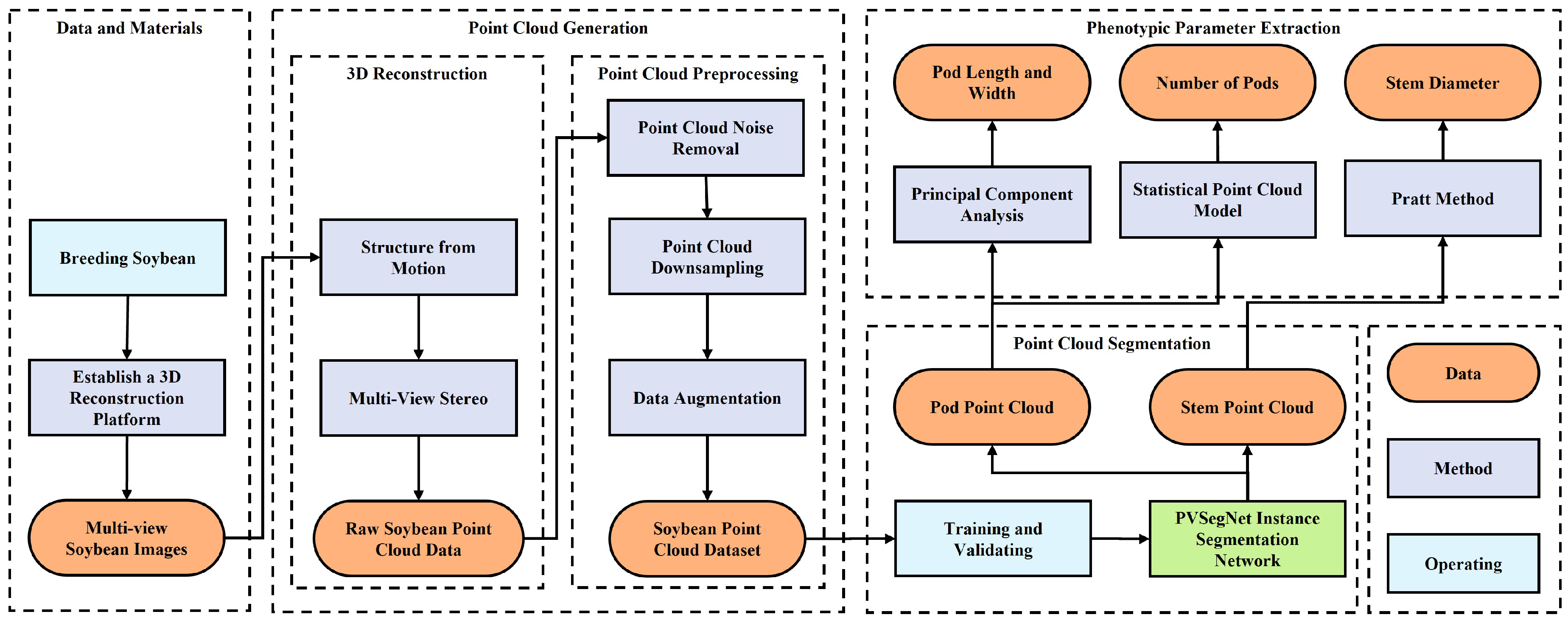
2. Materials and Methods

2.1. Soybean Experimental Samples

The experimental materials were planted at the experimental base of Northeast Agricultural University in Harbin, Heilongjiang Province, China (45°36′ N, 126°18′ E). The experimental field for soybean cultivation is shown in Figure 1c. Mature soybeans harvested in 2023 served as the experimental material for phenotypic acquisition in this study. The potted planting method was as follows: two plants were grown per pot, with a spacing of 30 centimeters between pots. The sowing took place in mid-August, and the harvest was scheduled for mid-October. At the maturity stage of the soybeans, 60 plants were collected as experimental samples.

2.2. Point Cloud Data Generation

The method used in this study consists of four key stages: (1) the collection of materials and data, (2) the generation of 3D soybean point clouds, (3) the segmentation of pod and stem regions using a neural network, and (4) the extraction of soybean phenotypic parameters. Figure 2 provides a detailed overview of the methodological workflow, including the specific steps for extracting the soybean phenotypic parameters using point cloud data.

2.2.1. Image Acquisition

In this study, multi-view images of soybeans at different heights were collected (as shown in Figure 1b) for 3D reconstruction. This approach, compared to traditional fixed-height imaging, allows for a more complete capture of the soybean’s structural information [40]. To achieve 3D reconstruction of the soybean plants, we designed a 3D scanning platform that includes a Sony A7 camera, black light-absorbing cloth, tripod, motorized turntable, and lighting. The overlap rate of the captured images directly affects the accuracy of the reconstruction; a low overlap rate may lead to mismatched images and result in missing reconstructed areas [41]. We adjusted the height of the camera stand and the shooting angles, and controlled the speed of the turntable to determine the number of images taken. Due to the limited sensitivity of the camera’s image sensor, lighting played a crucial role in the experiment, helping to capture image details more effectively, with supplementary lights used for additional illumination. Excessive background, plant overlap, and dark areas are typically difficult to capture and increase the risk of 3D reconstruction failure [42]. We used black light-blocking cloth to eliminate shadows and background interference as shown in Figure 1a.

The soybean plants were placed on the turntable, and the rotation angle was controlled by adjusting the motor speed. Meanwhile, we manually adjusted the camera stand’s angle to capture images of the soybean plants from multiple perspectives. To maintain stability during the image capture process, the turntable paused rhythmically rather than rotating continuously. A photo was taken approximately every 6 degrees of rotation, resulting in 60 images per complete rotation. Next, the camera height was adjusted three times, from low to high, each time by one-third of the plant height. This process was repeated three times, resulting in three sets of rotational images from different angles, totaling 180 images. The image acquisition was conducted in a controlled laboratory environment to avoid interference from external factors such as lighting and wind. Each soybean plant took approximately 5 mi to photograph. After completing the image capture, we measured the phenotypic parameters of the soybean plants to validate the method proposed in this study. Using a ruler with a unit scale of 1 mm, the length and width of the soybean pods were measured. For the stem diameter, a vernier caliper with a unit scale of 0.01 mm was used.

2.2.2. Three-Dimensional Reconstruction

In this study, the 3D reconstruction of soybean plants was accomplished using multi-view soybean images and the Multi-view Stereo (MVS) [43] algorithm, generating the corresponding point cloud data. From the obtained image sequences, sparse point cloud data were recovered using the Structure-from-Motion (SFM) [44] method. Subsequently, we utilized the MVS algorithm to further reconstruct these sparse point clouds into dense point clouds. By combining the SFM and MVS algorithms, we effectively reconstructed the 3D structure of soybean plants from images taken at multiple angles, providing high-quality point cloud data to support subsequent analyses and applications. This method not only acquired 3D point cloud data but also provided reliable foundational data for training deep learning networks.

The SFM algorithm is a photogrammetric technique that estimates 3D structures from image sequences. Through these technical steps, we were able to accurately compute the intrinsic and extrinsic parameters of each image and generate sparse point clouds of the soybean plants. The MVS algorithm then utilized the calibrated images and the epipolar geometry of the original data to generate high-density point clouds, which were color-coded to produce the final dense point cloud data.

We used Agisoft Metashape (Agisoft LLC, St. Petersburg, Russia) to generate the required soybean point cloud data. Agisoft Metashape was applied for 3D reconstruction [45], as it is capable of processing high-quality image sequences and providing high-precision and high-quality reconstruction results. The software offers a comprehensive workflow, including photo alignment, feature extraction, feature matching, camera viewpoint calculation, and 3D point cloud reconstruction. To ensure the accuracy of the reconstruction, we adjusted the software parameters: the maximum feature count per image was set to 40,000, the image overlap was set to high, and the reconstruction accuracy was set to the highest level. Since Agisoft Metashape supports both GPU and CPU acceleration, it offers high speed and low time consumption during 3D reconstruction. The reconstruction process takes approximately 30 min per object. Upon completion, the point cloud data exported from Agisoft Metashape were in PLY (Polygon File Format) as shown in

Table 1. Description of soybean point cloud data obtained through 3D reconstruction.

Description	Value
Number of samples	60
Number of points	61.12 × ${10}^4$ − 68.58 × ${10}^4$
Plant coverage ([length, width, height])	min: [−2.56, −2.66, 12.00], max: [1.73, 2.19, 31.39]
Average pods proportion (%)	43.21

. The point cloud data file contains an M × 6 array, where M represents the number of points, and the 6 includes the X, Y, Z coordinates, and the red, green, and blue color channels.

Data annotation is a labor-intensive task, but it is crucial for the training of deep learning networks [46]. We used CloudCompare (version 2.12.4) software to manually select and remove the non-soybean parts to obtain clean soybean plant point cloud data. We adopted the standard format of the open-source dataset S3DIS [47] for annotating the soybean point cloud dataset. During manual annotation, we assigned semantic and instance labels to each point in the point cloud. The semantic annotation classified the point cloud into two categories: pods and stems. In the instance segmentation stage, each pod was individually labeled. The annotation file contains the original point cloud data along with the semantic and instance categories of each point for pods and stems. Figure 3 shows the process of annotating the soybean point cloud data using CloudCompare. Ultimately, the dataset contains 60 complete soybean point clouds and 1782 corresponding annotation files.

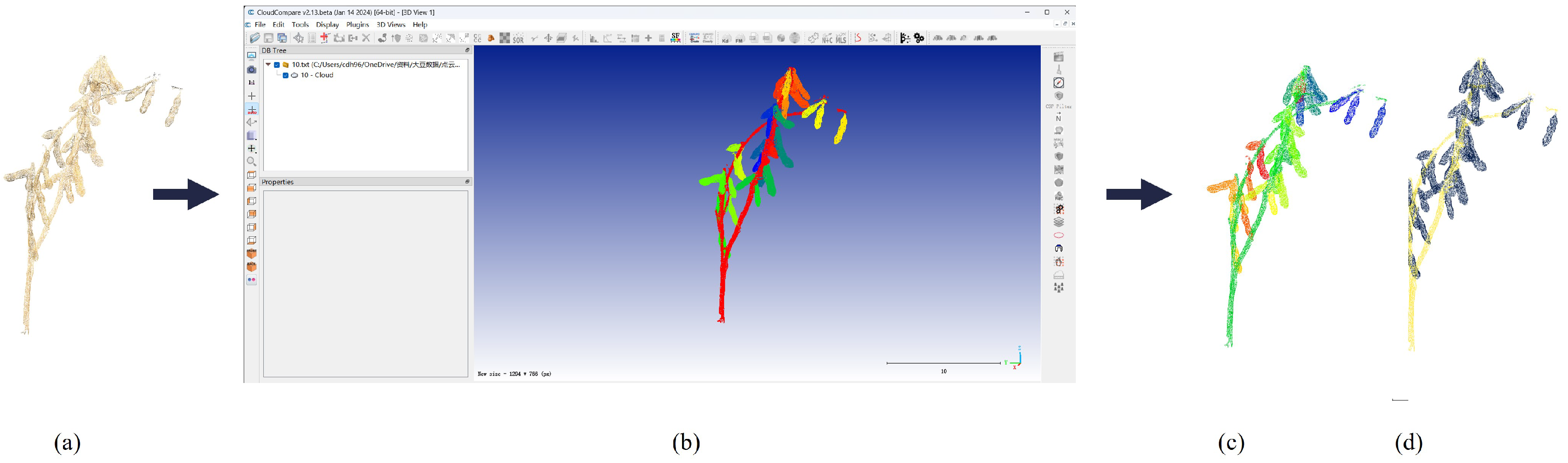
2.2.3. Point Cloud Preprocessing

After processing the multi-view soybean images with Agisoft Metashape, the resulting soybean plant point cloud models were very dense, with approximately 600,000 points per model. To ensure that the data were suitable for subsequent segmentation network training, we implemented the following point cloud preprocessing steps: (1) point cloud denoising to remove outliers from the soybean point cloud; (2) point cloud downsampling to retain the original distribution of the data while reducing point cloud density, thereby improving processing efficiency; and (3) data augmentation to expand the original dataset and enhance the network’s generalization ability and robustness.

Point Cloud Denoising

We employed radius filtering and statistical filtering to eliminate noise from the soybean point clouds [48]. Manually removing outliers can be challenging, but these filters effectively filter out point cloud noise. The radius filter exhibits superior performance in preserving shape and edges while offering fast processing speed, making it effective for handling large amounts of noise. On the other hand, the statistical filter leverages global statistical characteristics and is effective in removing minor noise.

Point Cloud Downsampling

Point cloud downsampling was primarily used to reduce the data volume and improve computational efficiency [49]. The uniform downsampling method [50] maintains the data distribution and essential feature information while reducing the point cloud density. Subsequently, we applied random downsampling [51] to standardize the number of points in the soybean point clouds. Initially, the point cloud data contained around 600,000 points, which we ultimately downsampled to 10,240 points per soybean plant.

Data Augmentation

Theoretically, data augmentation methods can significantly enhance the robustness and generalization ability of the network [52]. During the 3D reconstruction process, point clouds may encounter issues such as partial loss, coordinate system shifts, and scale variations [53]. To address these challenges, we applied global data augmentation methods such as scaling, cropping, rotation, and translation (Figure 4). These augmentation techniques increased the diversity and richness of the data, allowing the network to better adapt to various environmental changes [54]. By using these data augmentation methods, we expanded the original point cloud dataset, generating a dataset of 300 samples for training and testing the soybean organ segmentation network. The preprocessed soybean point clouds underwent the four data augmentation techniques sequentially, resulting in an expanded soybean point cloud dataset.

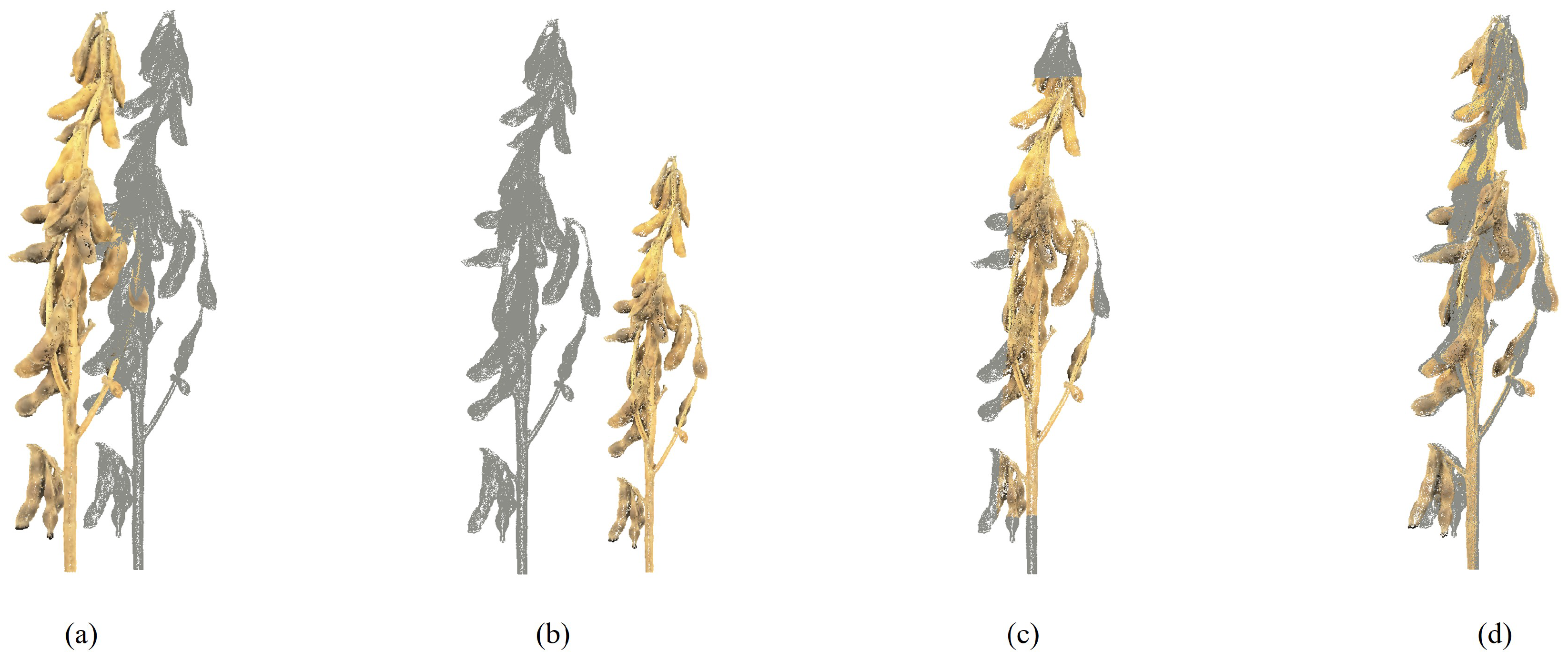
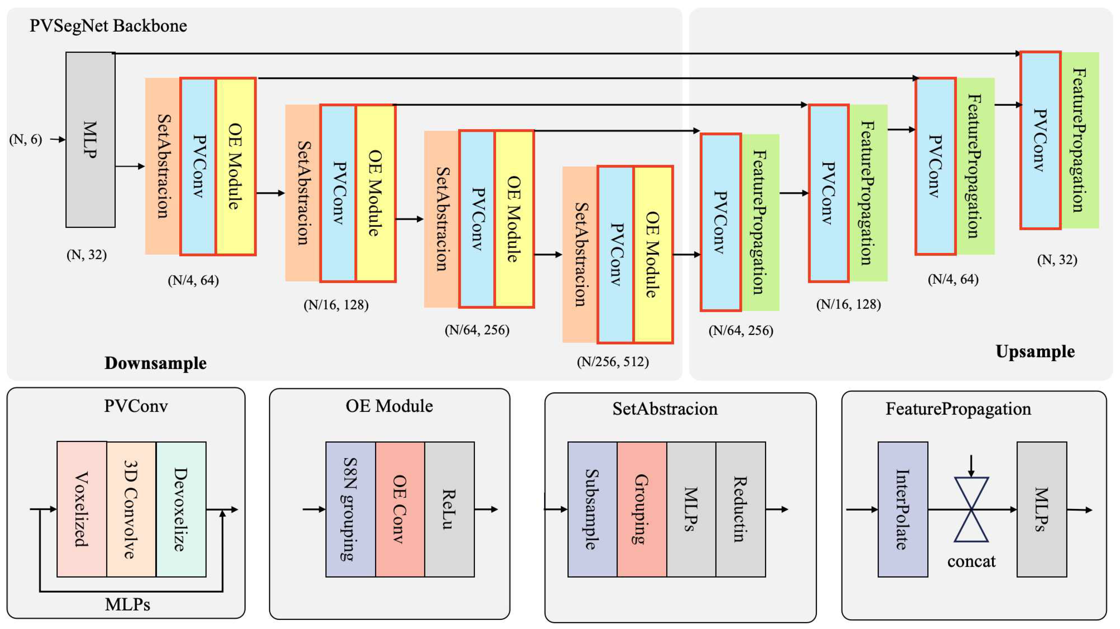
2.3. Point Cloud Segmentation

2.3.1. Network Architecture

In the study of soybean plant point cloud segmentation, our goal is to achieve both the semantic and instance segmentation of pods and stems. This means that each point is not only assigned a semantic label but also given a specific instance ID for the corresponding pod. We designed an end-to-end instance segmentation network for soybean organ segmentation, with the network architecture PVSegNet, illustrated in Figure 5. The network integrates PVConv [55] and orientation-encoding (OE) [56] modules into a PointNet++ framework to enhance feature extraction. This helps address the challenges posed by the irregularity and dispersion of pods and stems, thereby enhancing the accuracy of the semantic segmentation. The design of the feature extraction network is shown in Figure 6. We incorporated the PointGroup method to achieve the end-to-end instance segmentation of soybean plants.

PVConv [55] employs a point-voxel convolutional neural network that enhances network performance by combining point-based and voxel-based representations. The PVConv module integrates the advantages of point-based methods, which have lower memory usage, and voxel-based methods, which are beneficial for local feature regularity. This module improves the efficiency and effectiveness of each branch through fine-grained feature transformation and coarse-grained neighborhood aggregation. As shown in Figure 6, the PVConv module includes two branches: one generates a voxel-based feature map for the input point cloud, and the other produces a point-based feature map. These features are fused via an addition operation to produce the output of the PVConv module. In the voxelization branch, the point cloud is first voxelized through a voxelization module, followed by 3D convolution to extract features, and de-voxelization is used to merge with the point cloud features. Finally, these features are fused with the point cloud branch through multi-layer perceptron (MLP) layers. In this study, we replaced the MLP layers in the original PointNet++ with the PVConv module to simultaneously extract features from both voxel and point cloud data, enhancing the model’s feature extraction capability.

The orientation-encoding (OE) module [56] in the PointSIFT network plays a critical role in enhancing neighborhood information extraction, serving as a core component of the network. In simple terms, the OE module encodes information from eight different directions, helping the network better understand the local features. The internal structure of the OE module is shown in Figure 6. This module encodes information from eight directions using point-wise descriptors to improve the expression of the local features. Specifically, the OE module employs stacked 8-neighborhood (S8N) searches, identifying the nearest neighbors within an octant to generate a 2 × 2 × 2 cube that describes the local features. Subsequently, the cube undergoes three levels of OE convolution along the X, Y, and Z axes, integrating information from eight spatial directions to form a representation encoding directional information. In this study, we added the OE module to the downsampling part of the network to enhance the network’s ability to extract local features.

In the current research, methods for plant organ segmentation include direct clustering for segmentation or using clustering methods after semantic segmentation. These methods often require manual parameter setting and adjustments for different environments [57,58]. Meanwhile, PointGroup [59] is a two-stage network that can be integrated with PVSegNet to achieve the instance segmentation of soybean organs. To simplify the segmentation process, we employed PointGroup, an end-to-end segmentation method, wherein the PVSegNet network is constructed, with the network first receiving point cloud data X and extracting features F through the PVsegNet network. The features are then fed into two branches: semantic and offset module. In the semantic branch, features F pass through MLP layers and are converted into semantic labels S via Argmax operation. In the offset branch, the purpose of the offset module is to shift each point toward the center of its instance, thereby enabling the identification of individual instances. The offset module [59] computes the offset vector O for each point, which is added to the original coordinates P from X to obtain the offset coordinates Q. This aims to align each point to the centroid of its instance. The adjusted coordinates P and Q are grouped into candidate clusters $C^P$ and $C^Q$ using a clustering method [59]. This clustering process creates spherical regions, where adjacent points are clustered together. When points within a sphere have pod or stem labels, they are grouped as a corresponding instance. The union of $C^P$ and $C^Q$ forms the final clustering result C. Next, F and C are processed through ScoreNet [59] to calculate the score $S_c$ for each candidate instance.

During the training phase, the loss function comprises four components: semantic segmentation loss, offset branch regression loss, offset branch direction loss, and ScoreNet loss. The semantic segmentation loss and ScoreNet loss are calculated using a cross-entropy loss function. The semantic branch classifies each point to compute its loss, with the specific loss function expression as follows, where N is the total number of points, C is the number of semantic categories, $y_{i,c}$ is the true class label of the i-th point, and $p_{i,c}$ is the predicted probability that the i-th point belongs to class c:

$$L_{c\_sem}=-{\displaystyle \frac{1}{N}}\sum _{i=1}^N\sum _{c=1}^C{y}_{i,c}log\left(p_{i,c}\right)$$

(1)

The offset branch learns the offset vector from each point to the centroid of its corresponding instance, with two loss functions as follows, where $o_i$ is the predicted offset vector for the i-th point, and $\widehat{o_i}$ is the true offset vector for the i-th point:

$$L_{o\_reg}={\displaystyle \frac{1}{N}}\sum _{i=1}^N{\Vert o_i-\widehat{o_i}\Vert }_1$$

(2)

$$L_{o\_dir}={\displaystyle \frac{1}{N}}\sum _{i=1}^N\left(1-{\displaystyle \frac{o_i·\widehat{o_i}}{\Vert o_i\Vert \Vert \widehat{o_i}\Vert }}\right)$$

(3)

ScoreNet is responsible for predicting the score of the candidate clusters, with the loss function as follows, where M is the number of candidate clusters, $y_j$ is the true label of the j-th cluster (1 for valid clusters, 0 for invalid clusters), and $p_j$ is the predicted probability that the j-th cluster is valid:

$$L_{c\_score}=-{\displaystyle \frac{1}{M}}\sum _{j=1}^M\left[y_{j}log\left(p_j\right)+\left(1-y_j\right)log\left(1-p_j\right)\right]$$

(4)

By combining the above loss functions, the total loss function of the network is

$$L=L_{c\_sem}+L_{o\_reg}+L_{o\_dir}+L_{c\_score}$$

(5)

During the inference phase, Non-Maximum Suppression (NMS) is applied to C and the obtained scores $S_c$ to filter out low-quality clusters, resulting in the final instance segmentation output G.

2.3.2. Evaluation Metrics

The network’s performance is primarily evaluated in terms of instance segmentation and semantic segmentation. For semantic segmentation analysis, quantitative metrics such as precision (Prec), recall (Rec), F1-score, and Intersection over Union (IoU) are used. Here, $TP$, $FP$, and $FN$ represent true positives, false positives, and false negatives, respectively, and n represents the number of instances:

$$\mathrm{Prec}={\displaystyle \frac{TP}{TP+FP}}$$

(6)

$$\mathrm{Rec}={\displaystyle \frac{TP}{TP+FN}}$$

(7)

$$F_1-\mathrm{score}={\displaystyle \frac{2\times \mathrm{Prec}\times \mathrm{Rec}}{\mathrm{Prec}+\mathrm{Rec}}}$$

(8)

$$\mathrm{IoU}={\displaystyle \frac{TP}{TP+FP+FN}}$$

(9)

In instance segmentation, the performance of soybean organ instance segmentation is evaluated using average precision (AP) and average recall (AR). The metrics AP@25, AP@50, AR@25, and AR@50 [59] indicate the scores when the IoU threshold is set to 25% and 50%, respectively.

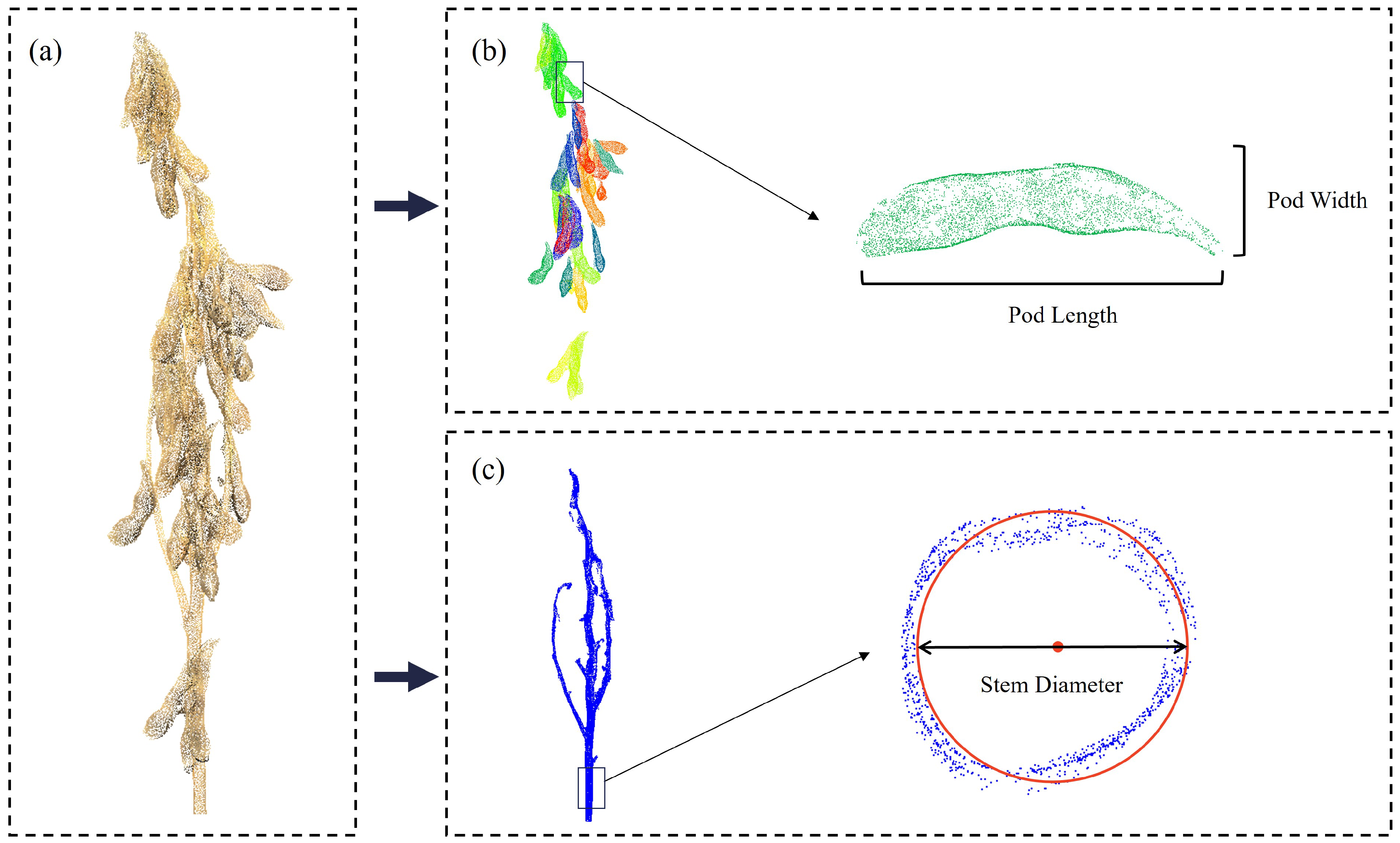
2.4. Morphological Parameter Extraction

Based on the soybean point cloud data, we used the network to extract the point cloud regions corresponding to the soybean stem and pods and then determined the phenotypic parameters such as pod length, pod width, and stem diameter using specific methods. The processing workflow is illustrated in Figure 7. To extract the stem diameter, we selected the points within the lowest 1 cm region of the main stem. These points were projected onto the $xy$ plane, and a circle was fitted using the Pratt method [60] to calculate the diameter, thus obtaining the stem diameter. For the extraction of pod length and width, we first performed principal component analysis (PCA) to identify the three principal axes of each pod’s point cloud [61]. We marked the endpoints along the first principal axis and calculated the pod length by determining the shortest path between these endpoints. Next, we divided the pod point cloud into five sections along the first principal component vector. Within each section, we identified the endpoints along the second and third principal component vectors, with the longest shortest path defined as the pod width. Finally, we evaluated the accuracy of phenotypic trait extraction using the coefficient of determination ($R^2$) and root mean square error (RMSE), calculated by the following formulas:

$$R^2=1-{\displaystyle \frac{{\sum }_{i=1}^m{(e_i-{\widehat{e}}_i)}^2}{{\sum }_{i=1}^m{(e_i-{\overline{e}}_i)}^2}}$$

(10)

$$\mathrm{RMSE}=\sqrt{{\displaystyle \frac{1}{m}}\sum _{i=1}^m{\left(e_i-{\widehat{e}}_i\right)}^2}$$

(11)

where $e_i$ and ${\widehat{e}}_i$ represent the true and predicted values, ${\overline{e}}_i$ is the mean of the true values, and m represents the number of samples being compared.

3. Results

3.1. Experimental Setup

In our experiments, the augmented soybean point cloud data were divided into training, validation, and test sets in a 7:1:2 ratio. All experiments were conducted on NVIDIA GeForce RTX 3090 GPU, and the network was constructed and trained using the PyTorch library. The PVSegNet network structure is an improved version based on PointNet++, with ReLU as the activation function. The input and output channels are shown in Figure 6, while other parameters use the default settings of the module. Before being fed into the network, each channel of the data was normalized. As shown in

Table 2. Network training parameter settings.

Parameter	Value
Batch Size	4
Epochs	300
Learning Rate	0.01
Optimizer	Adam
Momentum	0.9

, the training parameters were set with the Adam optimizer, and the network was trained for a total of 300 epochs, with a batch size of 4. The learning rate was initially set to 0.01 and optimized using cosine annealing. The weight decay set to 0.0001. We retained the network parameters corresponding to the epoch with the highest IoU on the validation set for subsequent performance testing. Additionally, the random seed was fixed to ensure the reproducibility of the experiments.

3.2. Ablation Study on the Effectiveness of the Method

To validate the effectiveness of each module in the method, an ablation study was conducted, with the results presented in

Table 3. Ablation study on the newly added modules. The best average class results are shown in bold, and the second best are underlined.

Method		IoU(%)	Prec (%)	Rec (%)	F1-Score (%)
Baseline	Stem	87.80	93.86	93.15	93.50
	Pod	93.65	96.54	96.91	96.72
	Mean	90.73	95.20	95.03	95.11
+PVConv	Stem	88.26	95.06	95.51	95.28
	Pod	93.98	96.25	94.46	95.35
	Mean	91.12	95.65	94.98	95.31
+OE	Stem	91.91	95.22	96.17	95.69
	Pod	90.13	94.96	94.42	94.69
	Mean	91.02	95.09	95.30	95.19
+PVConv + OE	Stem	89.51	96.47	92.54	94.46
	Pod	94.70	96.29	98.28	97.28
	Mean	92.10	96.38	95.41	95.87

. The table shows the impact of adding each module on the network’s performance. With the addition of modules, the model’s performance steadily improved. After adding the PVConv module, the mIoU increased by 0.39%, Prec increased by 0.45%, Rec decreased by 0.05%, and F1-score increased by 0.2%. After adding the OE module, the IoU increased by 0.29%, Prec decreased by 0.11%, Rec increased by 0.27%, and F1-score increased by 0.08%. When both the PVConv and OE modules were added, the final network was improved compared to the network with only the PVConv module, which showed a decrease in Prec, and the network with only the OE module, which showed a decrease in Rec. Ultimately, Prec increased by 1.18% and Rec increased by 0.38%.

3.3. Segmentation Results and Comparison

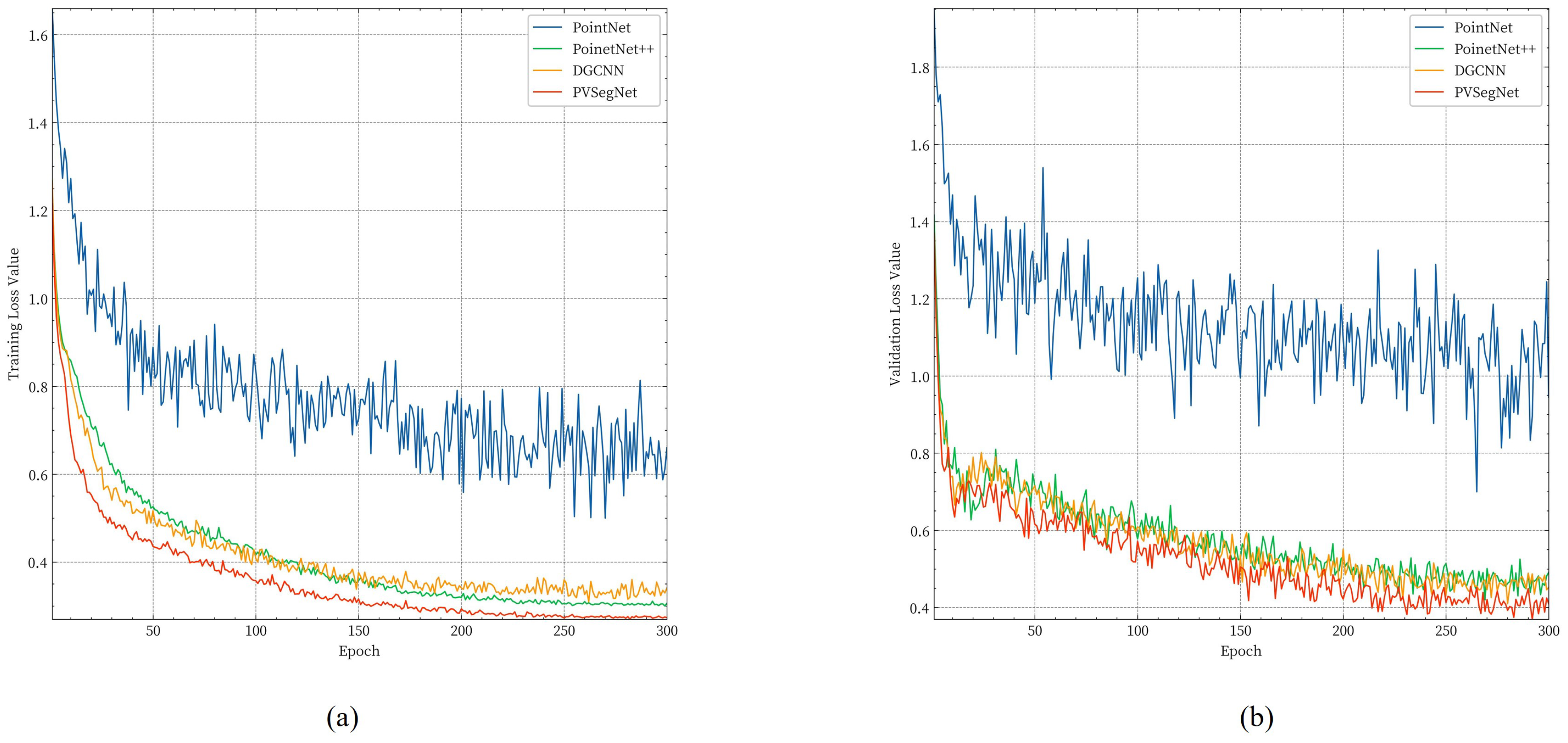
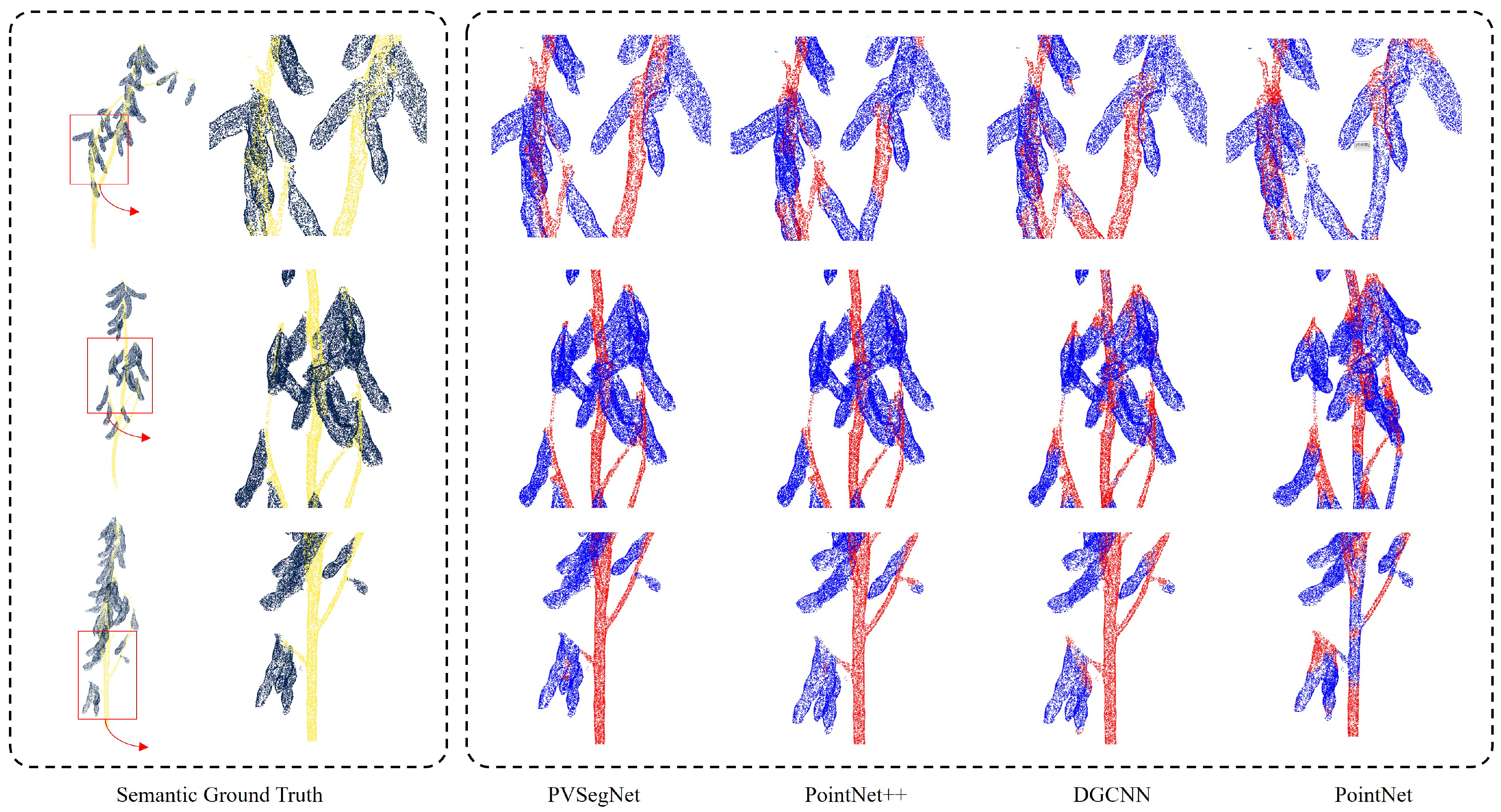
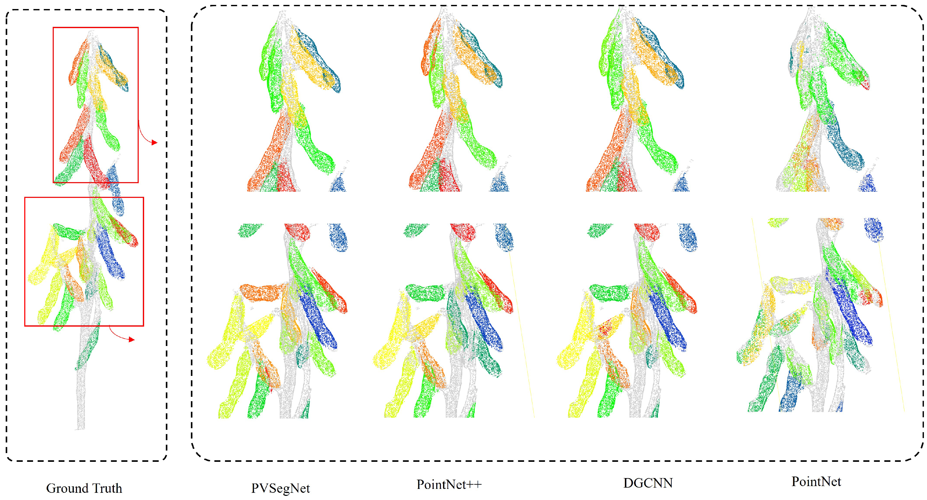
3.3.1. Comparison of Semantic Segmentation Methods

This section compares the proposed PVSegNet network with commonly used point cloud semantic segmentation networks, including PointNet [30], PointNet++ [62], and DGCNN [63]. All networks were trained on the same dataset using identical data augmentation techniques and hyperparameter configurations. To evaluate the performance of each network, we analyzed the loss function variations during the training and validation phases, as shown in Figure 8. We observed that the loss function value of PointNet was highly unstable during training. In contrast, the loss values for the other networks decreased rapidly within the first 120 epochs, then gradually stabilized, and leveled off after 200 epochs. Among all networks, PVSegNet exhibited the lowest loss values during both training and validation, indicating better generalization performance on the validation set.

According to

Table 4. Comparison of semantic segmentation results for the four networks. The best average class results are shown in bold.

Method		IoU (%)	Prec (%)	Rec (%)	F1-Score (%)
PointNet	Stem	48.38	70.40	62.31	62.64
	Pod	78.51	85.62	90.44	87.96
	Mean	58.96	78.81	70.07	74.18
PointNet++	Stem	87.80	93.86	93.15	93.50
	Pod	93.65	96.54	96.91	96.72
	Mean	90.73	95.20	95.03	95.11
DGCNN	Stem	92.13	93.90	98.00	95.90
	Pod	84.13	95.68	87.45	91.38
	Mean	88.13	94.79	92.72	93.64
PVSegNet (Ours)	Stem	89.51	96.47	92.54	94.46
	Pod	94.70	96.29	98.28	97.28
	Mean	92.10	96.38	95.41	95.87

, PVSegNet demonstrated the best performance, achieving the highest mIoU (92.10%), Prec (96.38%), Rec (95.41%), and F1-score (95.87%). Compared to PointNet++, PVSegNet improved by 1.47% in mIoU, 1.18% in Prec, 0.38% in Rec, and 0.76% in F1-score. As a graph-based method, DGCNN achieved the results of mIoU 88.13%, Prec 92.47%, Rec 92.72%, and F1-score 93.64%. PointNet performed the worst, with an mIoU of only 58.96%, likely due to its inability to effectively extract local features, making it difficult to accurately identify stems and pods. Figure 9 presents the semantic segmentation predictions of soybean pods and stems in the test set using the four methods. Visually, the primary differences in prediction results are observed in the connections between pods and stems and in dense pod areas. The PointNet network misclassified the regions of pods and stems, while the other networks made classification errors at the boundaries. The predictions of PVSegNet were the closest to the ground truth, showing sharper perception and significant advantages, particularly in detailed and edge regions.

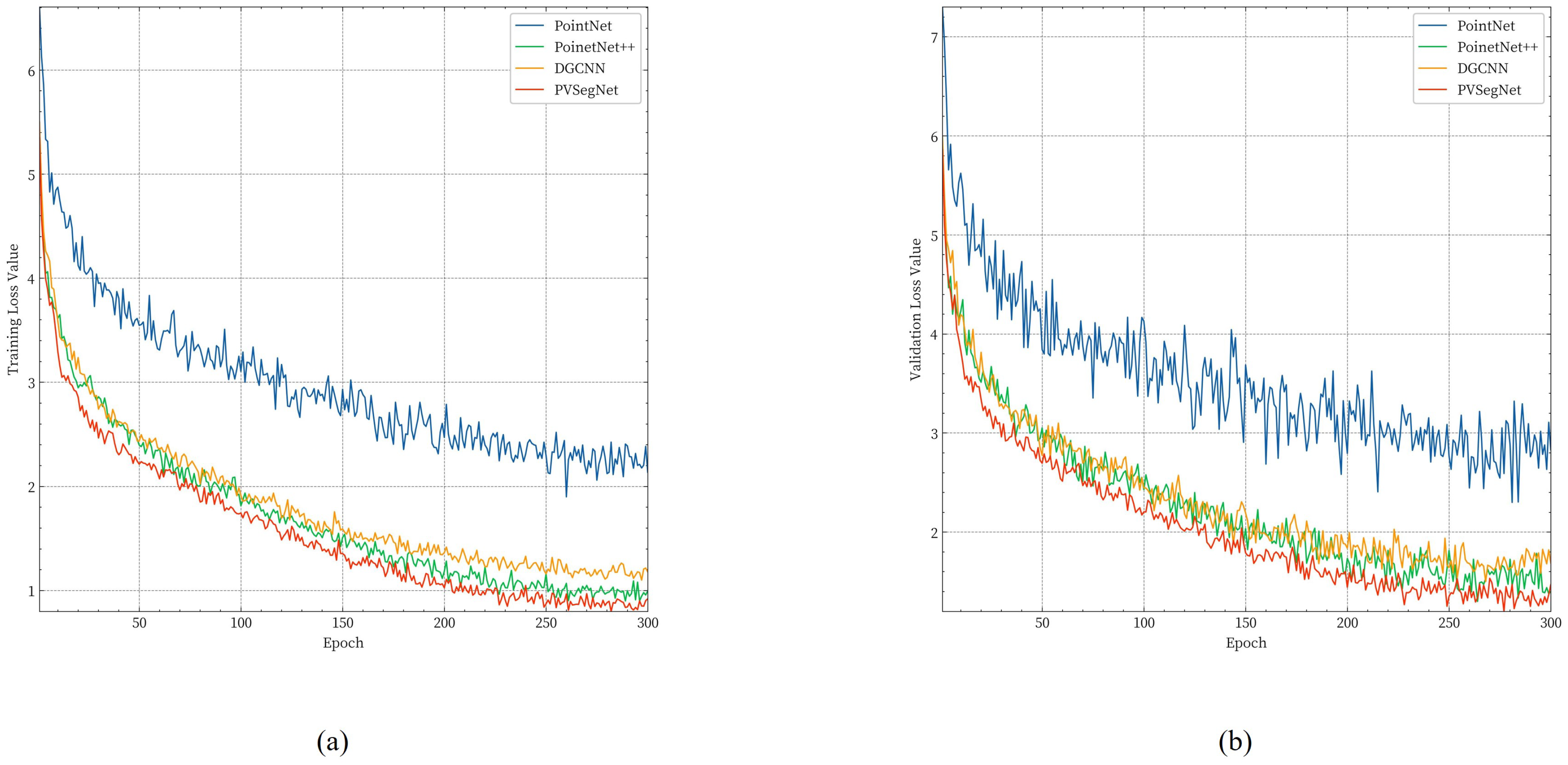
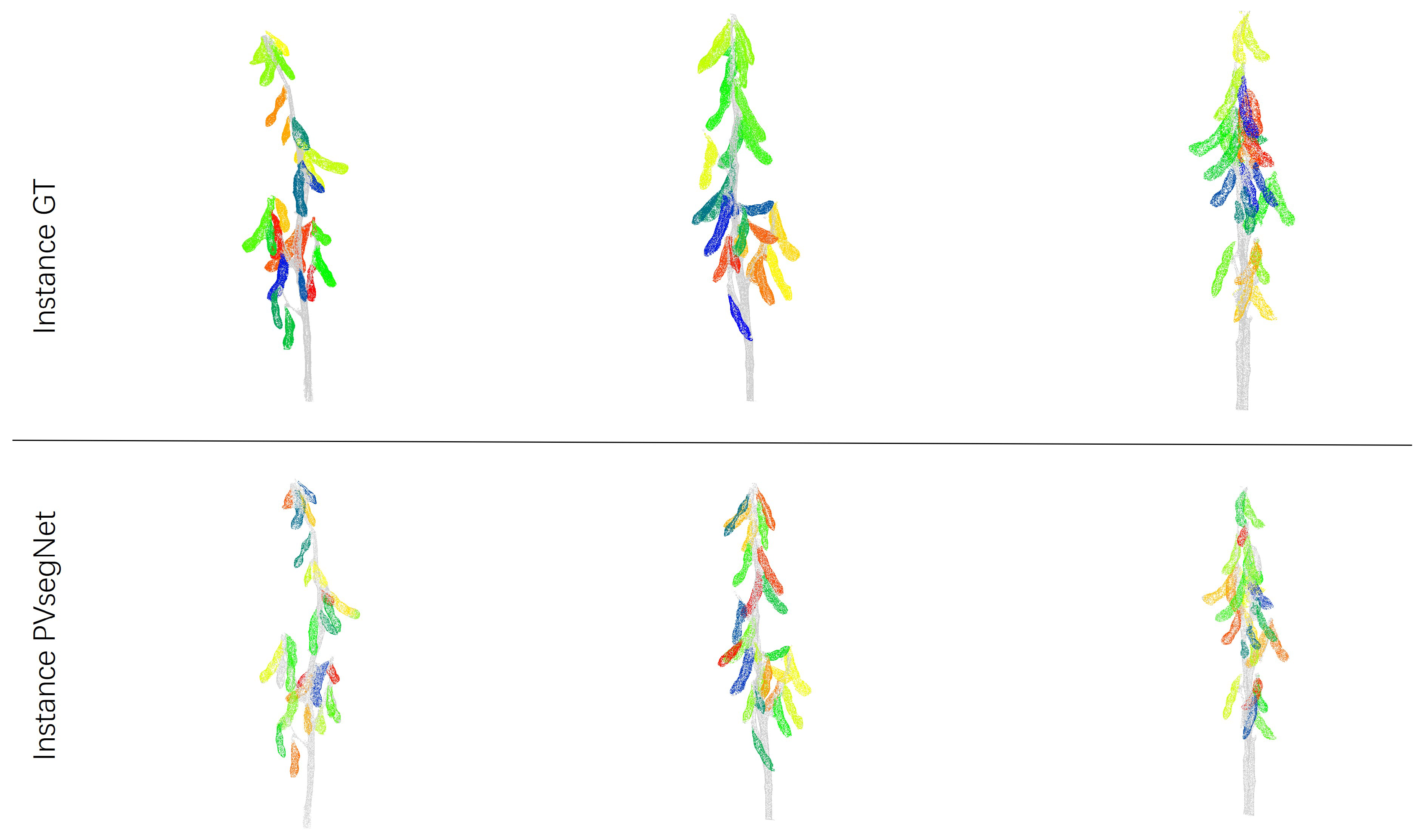
3.3.2. Comparison of Instance Segmentation Methods

This section presents the performance of the PointNet, PointNet++, DGCNN, and PVSegNet networks on the instance segmentation task. Figure 10 shows the changes in loss values during the training and validation phases. The four networks were tested on instance segmentation using the PointGroup algorithm, and to ensure fairness, default parameters were used for both training and testing. According to the results in

Table 5. Comparison of instance segmentation results for the four networks. The best average class results are shown in bold.

Method		AP@50 (%)	AP@25 (%)	AR@50 (%)	AR@25 (%)
PointNet	Stem	41.23	61.83	42.09	55.45
	Pod	40.07	52.48	63.89	88.89
	Mean	40.65	57.15	52.99	72.17
DGCNN	Stem	83.00	91.25	83.33	91.67
	Pod	69.73	75.51	70.20	75.58
	Mean	76.37	83.38	76.77	83.62
PointNet++	Stem	74.97	98.02	86.79	89.86
	Pod	86.75	89.54	86.11	97.22
	Mean	80.86	93.78	86.45	93.54
PVSegNet (Ours)	Stem	78.97	97.96	86.12	90.17
	Pod	87.97	90.15	88.02	97.23
	Mean	83.47	94.06	87.07	93.70

, PVSegNet performed the best, achieving an AP@50 of 83.47%, AP@25 of 94.06%, AR@50 of 87.07%, and AR@25 of 93.70%. Compared to PointNet++, the AP@50, AP@25, AR@50, and AR@25 improved by 2.61%, 0.28%, 0.62%, and 0.16%, respectively. PointNet performed the worst, with an AP@50 of 40.65% and an AR@50 of 52.99%, highlighting the impact of the semantic segmentation results on instance segmentation outcomes. The graph-based DGCNN network achieved an AP@50 of 76.37% and an AR@50 of 76.77%. The instance segmentation prediction results of PVSegNet are visualized in Figure 11 and Figure 12. The prediction results of the PointNet network showed significant errors in instance segmentation due to the impact of semantic segmentation. In the PointNet++ and DGCNN networks, pods were segmented as instances, but there were areas at the overlaps and edges that were incorrectly identified as stems. The PVSegNet results closely matched the annotations, providing a reliable data source for subsequent phenotypic extraction.

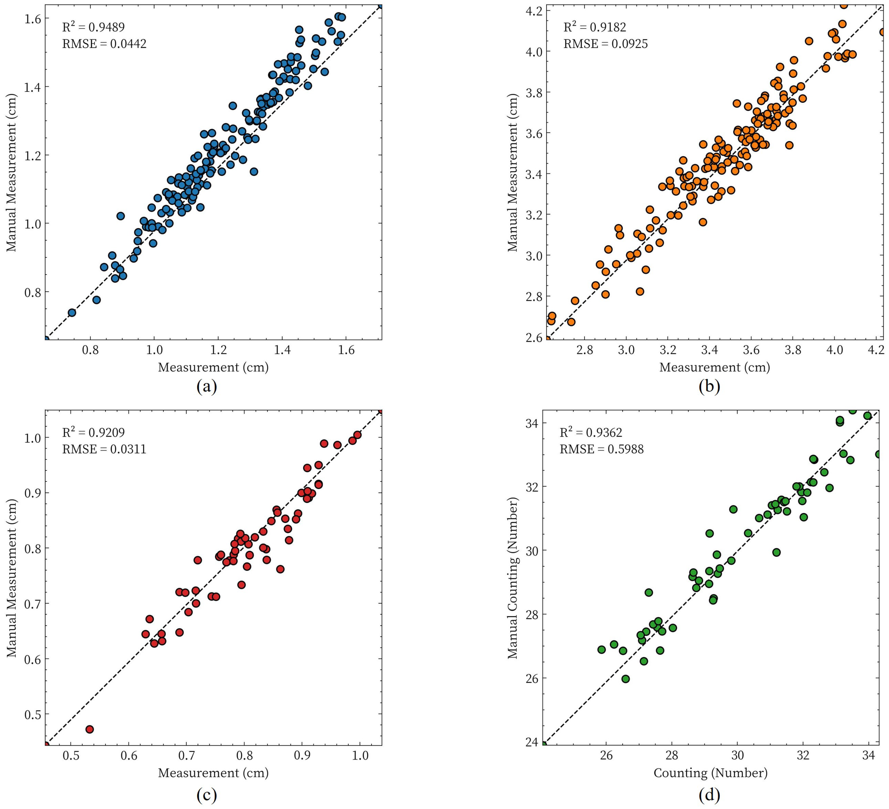
3.4. Results of Phenotypic Parameter Extraction

We evaluated the accuracy of the proposed method for extracting pod and stem phenotypic parameters by comparing the point cloud segmentation results with manual measurements. For the experimental materials, the numbers of pods and stem diameters were measured for 60 soybean plants. Additionally, 150 pods were randomly sampled to compare their lengths and widths. As shown in Figure 13d, the validation results for pod count show an $R^2$ of 0.9362 and an RMSE of 0.5988. Figure 13a–c display the validation results for the pod width, length, and stem thickness, with $R^2$ values of 0.9489, 0.9182, and 0.9209, respectively, and RMSE values of 0.0442 cm, 0.0925 cm, and 0.0311 cm, respectively. The evaluation results for pod length were lower compared to those for the pod width. These results indicate that the proposed method can meet the requirements for automated phenotypic parameter extraction.

4. Discussion

4.1. Point Cloud Generation

The generation of high-quality point clouds has been shown to enhance the performance of neural networks, alleviate the challenges of point cloud segmentation, and improve the accuracy of phenotypic extraction results [64]. In this study, we designed a multi-view acquisition scheme and utilized a custom-built platform to obtain multi-view images. Through multi-view 3D reconstruction technology, we successfully constructed a high-quality soybean point cloud dataset that meets the requirements for phenotypic parameters acquisition. However, environmental factors and the degree of image overlap during the reconstruction process affected the reconstruction quality, leading to potential errors in subsequent processing. To improve the quality of reconstruction, we controlled lighting and background conditions to minimize the interference from external environmental factors. Variations and insufficiencies in lighting can cause difficulties in image feature matching during reconstruction, which in turn affects the clear display of plant features. In constructing the multi-view acquisition platform, we used black light-absorbing cloth as the background to eliminate plant shadows and ensure that only the object of interest appeared in the images. The primary goal of this approach was to minimize interference from external objects on the reconstruction accuracy. By adjusting the shooting height and the interval of the turntable captures, we enhanced the overlap of image acquisition, thereby ensuring the quality of the reconstruction.

4.2. Downsampling the Number of Point Clouds

The number of points in a point cloud significantly impacts the performance of deep learning networks. A larger number of points generally improves the accuracy and completeness of the network but also increases the computational complexity and storage requirements [65,66]. To select an appropriate number of points that balance accuracy and speed, we employed a random downsampling method to reduce the point cloud to different quantities (4096, 6144, 10,240, and 12,288 points). Semantic segmentation experiments were conducted with a batch size of 4, while other parameters were kept consistent with Section 3.1. The results shown in

Table 6. Semantic segmentation results of PVSegNet on different numbers of points.

Number of Points	mIoU (%)	Throughput (Items/s)
6144	88.97	117.11
8192	91.02	84.92
10,240	92.10	65.27
12,288	92.23	52.50

indicate that increasing the number of downsampled points positively affects network performance. This improvement can be attributed to the enhanced information and feature density [63], enabling the network to capture more complex details. Due to computational limitations, we did not test inputs with a higher number of points. It is noteworthy that as the number of points increases, the inference speed of the network tends to decrease to prioritize higher accuracy in order to achieve a balance between precision and speed. Therefore, in practical applications, it is crucial to choose the number of downsampled points that optimizes the balance between network prediction accuracy and efficiency, taking into account the available computational capacity determined by the hardware configuration.

4.3. Future Work

This study has validated the feasibility of extracting phenotypic parameters of soybean pods and stems based on 3D segmentation algorithms. The proposed PVSegNet significantly improved segmentation accuracy by combining point cloud and voxel features. Considering the hardware constraints and the need for real-time evaluation scenarios, future research will explore lightweight functional modules to enhance the inference speed of the network. Moreover, the diversity and scale of the dataset are crucial for network training. In subsequent research, we plan to expand the data samples by using different materials to further enhance the performance and robustness of the network, thereby providing greater potential value for the application of precision agriculture technologies.

5. Conclusions

In summary, this study developed a novel pipeline for acquiring the phenotypic traits of mature soybeans based on 3D point clouds and the proposed PVSegNet, a deep learning-based network integrating point cloud and voxel convolution to enhance feature extraction for segmenting soybean pods and stems. The experimental results demonstrated an IoU of 92.10%, precision of 96.38%, recall of 95.41%, and F1-score of 95.87% in semantic segmentation, and an AP@50 of 83.47% and AR@50 of 87.07% in instance segmentation. The validation results for pod width, length, and stem thickness showed $R^2$ values of 0.9489, 0.9182, and 0.9209, respectively. Future research will prioritize developing lightweight modules for faster inference and expanding diverse datasets to enhance network performance and precision agriculture applications. This study contributes to the field of plant phenotyping and provides valuable insights for the future development of precision agriculture technologies.

References

1. Jiang, G.; Chen, P.; Zhang, J.; Florez-Palacios, L.; Zeng, A.; Wang, X.; Bowen, R.A.; Miller, A.M.; Berry, H. Genetic Analysis of Sugar Composition and Its Relationship with Protein, Oil, and Fiber in Soybean. Crop Sci. 2018, 58, 2413–2421. [Google Scholar] [CrossRef]
2. Florou-Paneri, P.; Christaki, E.; Giannenas, I.; Bonos, E.; Skoufos, I.; Tsinas, A.; Tzora, A.; Peng, J. Alternative Protein Sources to Soybean Meal in Pig Diets. J. Food Agric. Environ. 2014, 12, 655–660. [Google Scholar]
3. Zhang, M.; Liu, S.; Wang, Z.; Yuan, Y.; Zhang, Z.; Liang, Q.; Yang, X.; Duan, Z.; Liu, Y.; Kong, F.; et al. Progress in Soybean Functional Genomics over the Past Decade. Plant Biotechnol. J. 2021, 20, 256–282. [Google Scholar] [CrossRef] [PubMed]
4. Bao, X.; Yao, X. Genetic Improvements in the Root Traits and Fertilizer Tolerance of Soybean Varieties Released during Different Decades. Agronomy 2023, 14, 2. [Google Scholar] [CrossRef]
5. Chang, F.; Lv, W.; Lv, P.; Xiao, Y.; Yan, W.; Chen, S.; Zheng, L.; Xie, P.; Wang, L.; Karikari, B.; et al. Exploring Genetic Architecture for Pod-Related Traits in Soybean Using Image-Based Phenotyping. Mol. Breed. 2021, 41, 28. [Google Scholar] [CrossRef] [PubMed]
6. Parmley, K.A.; Nagasubramanian, K.; Sarkar, S.; Ganapathysubramanian, B.; Singh, A.K. Development of Optimized Phenomic Predictors for Efficient Plant Breeding Decisions Using Phenomic-Assisted Selection in Soybean. Plant Phenomics 2019, 2019, 5809404. [Google Scholar] [CrossRef] [PubMed]
7. Chouhan, S.S.; Singh, U.; Jain, S. Applications of Computer Vision in Plant Pathology: A Survey. Arch. Comput. Methods Eng. 2020, 27, 611–632. [Google Scholar] [CrossRef]
8. Ngugi, L.C.; Abdelwahab, M.; Abo-Zahhad, M. Tomato Leaf Segmentation Algorithms for Mobile Phone Applications Using Deep Learning. Comput. Electron. Agric. 2020, 178, 105788. [Google Scholar] [CrossRef]
9. Miao, C.; Guo, A.; Thompson, A.M.; Yang, J.; Ge, Y.; Schnable, J.C. Automation of Leaf Counting in Maize and Sorghum Using Deep Learning. Plant Phenome J. 2021, 4, e20022. [Google Scholar] [CrossRef]
10. Zhang, Z.; Pope, M.; Shakoor, N.; Pless, R.; Mockler, T.; Stylianou, A. Comparing Deep Learning Approaches for Understanding Genotype × Phenotype Interactions in Biomass Sorghum. Front. Artif. Intell. 2022, 5, 872858. [Google Scholar] [CrossRef] [PubMed]
11. Li, R.; Wang, D.; Zhu, B.; Liu, T.; Sun, C.; Zhang, Z. Estimation of Nitrogen Content in Wheat Using Indices Derived from RGB and Thermal Infrared Imaging. Field Crops Res. 2022, 289, 108735. [Google Scholar] [CrossRef]
12. Wu, T.; Shen, P.; Dai, J.; Ma, Y.; Feng, Y. A Pathway to Assess Genetic Variation of Wheat Germplasm by Multidimensional Traits with Digital Images. Plant Phenomics 2023, 5, 119. [Google Scholar] [CrossRef] [PubMed]
13. Feldmann, M.J.; Tabb, A. Cost-Effective, High-Throughput Phenotyping System for 3D Reconstruction of Fruit Form. bioRxiv 2021. [Google Scholar] [CrossRef]
14. Wu, S.; Wen, W.; Gou, W.; Lu, X.; Zhang, W.; Zheng, C.; Xiang, Z.; Chen, L.; Guo, X. A Miniaturized Phenotyping Platform for Individual Plants Using Multi-View Stereo 3D Reconstruction. Front. Plant Sci. 2022, 13, 897746. [Google Scholar] [CrossRef] [PubMed]
15. Ziamtsov, I.; Navlakha, S. Plant 3D (P3D): A Plant Phenotyping Toolkit for 3D Point Clouds. Bioinformatics 2020, 36, 3949–3950. [Google Scholar] [CrossRef] [PubMed]
16. Qiu, Q.; Sun, N.; Bai, H.; Wang, N.; Fan, Z.; Wang, Y.; Meng, Z.; Li, B.; Cong, Y. Field-Based High-Throughput Phenotyping for Maize Plant Using 3D LiDAR Point Cloud Generated With a “Phenomobile”. Front. Plant Sci. 2019, 10, 554. [Google Scholar] [CrossRef] [PubMed]
17. Rivera, G.; Porras, R.; Florencia, R.; Sanchez-Solis, J.P. LiDAR Applications in Precision Agriculture for Cultivating Crops: A Review of Recent Advances. Comput. Electron. Agric. 2023, 207, 107737. [Google Scholar] [CrossRef]
18. Jin, S.; Sun, X.; Wu, F.; Su, Y.; Li, Y.; Song, S.; Xu, K.; Ma, Q.; Baret, F.; Jiang, D.; et al. Lidar Sheds New Light on Plant Phenomics for Plant Breeding and Management: Recent Advances and Future Prospects. ISPRS-J. Photogramm. Remote Sens. 2021, 171, 202–223. [Google Scholar] [CrossRef]
19. Song, P.; Li, Z.; Yang, M.; Shao, Y.; Pu, Z.; Yang, W.; Zhai, R. Dynamic Detection of Three-Dimensional Crop Phenotypes Based on a Consumer-Grade RGB-D Camera. Front. Plant Sci. 2023, 14, 1097725. [Google Scholar] [CrossRef] [PubMed]
20. Wang, H.; Duan, Y.; Shi, Y.; Kato, Y.; Ninomiya, S.; Guo, W. EasyIDP: A Python Package for Intermediate Data Processing in UAV-Based Plant Phenotyping. Remote Sens. 2021, 13, 2622. [Google Scholar] [CrossRef]
21. Sun, Y.; Zhang, Z.; Sun, K.; Li, S.; Yu, J.; Miao, L.; Zhang, Z.; Li, Y.; Zhao, H.; Hu, Z.; et al. Soybean-MVS: Annotated Three-Dimensional Model Dataset of Whole Growth Period Soybeans for 3D Plant Organ Segmentation. Agriculture 2023, 13, 1321. [Google Scholar] [CrossRef]
22. Luo, L.; Jiang, X.; Yang, Y.; Samy, E.R.A.; Lefsrud, M.; Hoyos-Villegas, V.; Sun, S. Eff-3DPSeg: 3D Organ-Level Plant Shoot Segmentation Using Annotation-Efficient Deep Learning. Plant Phenomics 2023, 5, 80. [Google Scholar] [CrossRef] [PubMed]
23. Lin, Y.; Ruifang, Z.; Pujuan, S.; Pengfei, W. Segmentation of Crop Organs through Region Growing in 3D Space. In Proceedings of the 2016 Fifth International Conference on Agro-Geoinformatics (Agro-Geoinformatics), Tianjin, China, 18–20 July 2016; pp. 1–6. [Google Scholar] [CrossRef]
24. Cuevas-Velasquez, H.; Gallego, A.J.; Fisher, R.B. Segmentation and 3D Reconstruction of Rose Plants from Stereoscopic Images. Comput. Electron. Agric. 2020, 171, 105296. [Google Scholar] [CrossRef]
25. Vo, A.; Truong-Hong, L.; Laefer, D.; Bertolotto, M. Octree-Based Region Growing for Point Cloud Segmentation. ISPRS J. Photogramm. Remote Sens. 2015, 104, 88–100. [Google Scholar] [CrossRef]
26. Han, H.; Han, X.; Gao, T. 3D Mesh Model Segmentation Based on Skeleton Extraction. Imaging Sci. J. 2021, 69, 153–163. [Google Scholar] [CrossRef]
27. Dutagaci, H.; Rasti, P.; Galopin, G.; Rousseau, D. ROSE-X: An Annotated Data Set for Evaluation of 3D Plant Organ Segmentation Methods. Plant Methods 2020, 16, 1–14. [Google Scholar] [CrossRef] [PubMed]
28. Chaudhury, A.; Ward, C.D.W.; Talasaz, A.; Ivanov, A.; Brophy, M.; Grodzinski, B.; Hüner, N.; Patel, R.V.; Barron, J. Machine Vision System for 3D Plant Phenotyping. IEEE/ACM Trans. Comput. Biol. Bioinform. 2017, 16, 2009–2022. [Google Scholar] [CrossRef] [PubMed]
29. Mostafa, S.; Mondal, D.; Panjvani, K.; Kochian, L.; Stavness, I. Explainable Deep Learning in Plant Phenotyping. Front. Artif. Intell. 2023, 6, 1203546. [Google Scholar] [CrossRef]
30. Charles, R.Q.; Su, H.; Kaichun, M.; Guibas, L.J. PointNet: Deep Learning on Point Sets for 3D Classification and Segmentation. In Proceedings of the 2017 IEEE Conference on Computer Vision and Pattern Recognition (CVPR), Honolulu, HI, USA, 21–26 July 2017; pp. 77–85. [Google Scholar] [CrossRef]
31. Li, Y.; Wen, W.; Miao, T.; Wu, S.; Yu, Z.; Wang, X.; Guo, X.; Zhao, C. Automatic Organ-Level Point Cloud Segmentation of Maize Shoots by Integrating High-Throughput Data Acquisition and Deep Learning. Comput. Electron. Agric. 2022, 193, 106702. [Google Scholar] [CrossRef]
32. Li, D.; Shi, G.; Li, J.; Chen, Y.; Zhang, S.; Xiang, S.; Jin, S. PlantNet: A Dual-Function Point Cloud Segmentation Network for Multiple Plant Species. ISPRS J. Photogramm. Remote Sens. 2022, 184, 243–263. [Google Scholar] [CrossRef]
33. Zhou, Y.; Tuzel, O. VoxelNet: End-to-End Learning for Point Cloud Based 3D Object Detection. In Proceedings of the 2018 IEEE/CVF Conference on Computer Vision and Pattern Recognition, Salt Lake City, UT, USA, 18–22 June 2018; pp. 4490–4499. [Google Scholar] [CrossRef]
34. Jin, S.; Su, Y.; Gao, S.; Wu, F.; Ma, Q.; Xu, K.; Ma, Q.; Hu, T.; Liu, J.; Pang, S.; et al. Separating the Structural Components of Maize for Field Phenotyping Using Terrestrial LiDAR Data and Deep Convolutional Neural Networks. IEEE Trans. Geosci. Remote Sens. 2020, 58, 2644–2658. [Google Scholar] [CrossRef]
35. Li, D.; Li, J.; Xiang, S.; Pan, A. PSegNet: Simultaneous Semantic and Instance Segmentation for Point Clouds of Plants. Plant Phenomics 2022, 2022. [Google Scholar] [CrossRef] [PubMed]
36. Mukherjee, S.; Lu, D.; Raghavan, B.; Breitkopf, P.; Dutta, S.; Xiao, M.; Zhang, W. Accelerating Large-scale Topology Optimization: State-of-the-Art and Challenges. Arch. Comput. Methods Eng. 2021, 28, 4549–4571. [Google Scholar] [CrossRef]
37. Howe, M.; Repasky, B.; Payne, T. Effective Utilisation of Multiple Open-Source Datasets to Improve Generalisation Performance of Point Cloud Segmentation Models. In Proceedings of the 2022 International Conference on Digital Image Computing: Techniques and Applications (DICTA), Sydney, Australia, 30 November–2 December 2022; pp. 1–7. [Google Scholar] [CrossRef]
38. Schunck, D.; Magistri, F.; Rosu, R.; Cornelissen, A.; Chebrolu, N.; Paulus, S.; Léon, J.; Behnke, S.; Stachniss, C.; Kuhlmann, H.; et al. Pheno4D: A Spatio-Temporal Dataset of Maize and Tomato Plant Point Clouds for Phenotyping and Advanced Plant Analysis. PLoS ONE 2021, 16, e0256340. [Google Scholar] [CrossRef]
39. Boogaard, F.P.; van Henten, E.J.; Kootstra, G. Improved Point-Cloud Segmentation for Plant Phenotyping Through Class-Dependent Sampling of Training Data to Battle Class Imbalance. Front. Plant Sci. 2022, 13, 838190. [Google Scholar] [CrossRef] [PubMed]
40. Zhu, B.; Liu, F.; Che, Y.; Hui, F.; Ma, Y. Three-Dimensional Quantification of Intercropping Crops in Field by Ground and Aerial Photography. In Proceedings of the 2018 6th International Symposium on Plant Growth Modeling, Simulation, Visualization and Applications (PMA), Hefei, China, 4–8 November 2018; pp. 1–5. [Google Scholar] [CrossRef]
41. Chakraborty, S.; Banerjee, A.; Gupta, S.; Christensen, P. Region of Interest Aware Compressive Sensing of THEMIS Images and Its Reconstruction Quality. In Proceedings of the 2018 IEEE Aerospace Conference, Big Sky, MT, USA, 3–10 March 2018; pp. 1–11. [Google Scholar] [CrossRef]
42. López-Torres, C.V.; Salazar-Colores, S.; Kells, K.; Ortega, J.; Arreguín, J.M.R. Improving 3D Reconstruction Accuracy in Wavelet Transform Profilometry by Reducing Shadow Effects. IET Image Process. 2020, 14, 310–317. [Google Scholar] [CrossRef]
43. Liu, Y.; Dai, Q.; Xu, W. A Point-Cloud-Based Multiview Stereo Algorithm for Free-Viewpoint Video. IEEE Trans. Vis. Comput. Graph. 2010, 16, 407–418. [Google Scholar] [CrossRef] [PubMed]
44. Condorelli, F.; Higuchi, R.; Nasu, S.; Rinaudo, F.; Sugawara, H. Improving Performance Of Feature Extraction In Sfm Algorithms For 3d Sparse Point Cloud. ISPRS Int. Arch. Photogramm. Remote Sens. Spat. Inf. Sci. 2019, 42, 101–106. [Google Scholar] [CrossRef]
45. Dascăl, A.; Popa, M. Possibilities of 3D Reconstruction of the Vehicle Collision Scene in the Photogrammetric Environment Agisoft Metashape 1.6.2. J. Physics: Conf. Ser. 2021, 1781, 012053. [Google Scholar] [CrossRef]
46. Kim, J.; Ko, Y.; Seo, J. Construction of Machine-Labeled Data for Improving Named Entity Recognition by Transfer Learning. IEEE Access 2020, 8, 59684–59693. [Google Scholar] [CrossRef]
47. Armeni, I.; Sener, O.; Zamir, A.R.; Jiang, H.; Brilakis, I.; Fischer, M.; Savarese, S. 3D Semantic Parsing of Large-Scale Indoor Spaces. In Proceedings of the IEEE Conference on Computer Vision and Pattern Recognition, Las Vegas, NV, USA, 27–30 June 2016; pp. 1534–1543. [Google Scholar]
48. Zhang, H.; Zhu, L.; Cai, X.; Dong, L. Noise Removal Algorithm Based on Point Cloud Classification. In Proceedings of the 2022 International Seminar on Computer Science and Engineering Technology (SCSET), Indianapolis, IN, USA, 8–9 January 2022; pp. 93–96. [Google Scholar] [CrossRef]
49. Wu, Z.; Zeng, Y.; Li, D.; Liu, J.; Feng, L. High-Volume Point Cloud Data Simplification Based on Decomposed Graph Filtering. Autom. Constr. 2021, 129, 103815. [Google Scholar] [CrossRef]
50. Chen, S.; Wang, J.; Pan, W.; Gao, S.; Wang, M.; Lu, X. Towards Uniform Point Distribution in Feature-Preserving Point Cloud Filtering. Comput. Vis. Media 2022, 9, 249–263. [Google Scholar] [CrossRef]
51. Zhou, J.; Fu, X.; Zhou, S.; Zhou, J.; Ye, H.; Nguyen, H. Automated Segmentation of Soybean Plants from 3D Point Cloud Using Machine Learning. Comput. Electron. Agric. 2019, 162, 143–153. [Google Scholar] [CrossRef]
52. Cortés-Ciriano, I.; Bender, A. Improved Chemical Structure-Activity Modeling Through Data Augmentation. J. Chem. Inf. Model. 2015, 55 12, 2682–2692. [Google Scholar] [CrossRef]
53. Wang, M.; Ju, M.; Fan, Y.; Guo, S.; Liao, M.; Yang, H.j.; He, D.; Komura, T. 3D Incomplete Point Cloud Surfaces Reconstruction With Segmentation and Feature-Enhancement. IEEE Access 2019, 7, 15272–15281. [Google Scholar] [CrossRef]
54. Xin, B.; Sun, J.; Bartholomeus, H.; Kootstra, G. 3D Data-Augmentation Methods for Semantic Segmentation of Tomato Plant Parts. Front. Plant Sci. 2023, 14, 1045545. [Google Scholar] [CrossRef] [PubMed]
55. Liu, Z.; Tang, H.; Lin, Y.; Han, S. Point-Voxel CNN for Efficient 3D Deep Learning. arXiv 2019, arXiv:cs/1907.03739. [Google Scholar]
56. Jiang, M.; Wu, Y.; Zhao, T.; Zhao, Z.; Lu, C. PointSIFT: A SIFT-like Network Module for 3D Point Cloud Semantic Segmentation. arXiv 2018, arXiv:cs/1807.00652. [Google Scholar]
57. Magistri, F.; Chebrolu, N.; Stachniss, C. Segmentation-Based 4D Registration of Plants Point Clouds for Phenotyping. In Proceedings of the 2020 IEEE/RSJ International Conference on Intelligent Robots and Systems (IROS), Las Vegas, NV, USA, 25–29 October 2020; pp. 2433–2439. [Google Scholar] [CrossRef]
58. Wahabzada, M.; Paulus, S.; Kersting, K.; Mahlein, A.K. Automated Interpretation of 3D Laserscanned Point Clouds for Plant Organ Segmentation. BMC Bioinform. 2015, 16, 1–11. [Google Scholar] [CrossRef]
59. Jiang, L.; Zhao, H.; Shi, S.; Liu, S.; Fu, C.W.; Jia, J. PointGroup: Dual-Set Point Grouping for 3D Instance Segmentation. In Proceedings of the 2020 IEEE/CVF Conference on Computer Vision and Pattern Recognition (CVPR), Seattle, WA, USA, 13–19 June 2020; pp. 4866–4875. [Google Scholar] [CrossRef]
60. Saeed, F.; Sun, S.; Rodriguez-Sanchez, J.; Snider, J.; Liu, T.; Li, C. Cotton plant part 3D segmentation and architectural trait extraction using point voxel convolutional neural networks. Plant Methods 2023, 19, 33. [Google Scholar] [CrossRef]
61. Miao, T.; Zhu, C.; Xu, T.; Yang, T.; Li, N.; Zhou, Y.; Deng, H. Automatic Stem-Leaf Segmentation of Maize Shoots Using Three-Dimensional Point Cloud. Comput. Electron. Agric. 2021, 187, 106310. [Google Scholar] [CrossRef]
62. Qi, C.R.; Yi, L.; Su, H.; Guibas, L.J. Pointnet++: Deep hierarchical feature learning on point sets in a metric space. Adv. Neural Inf. Process. Syst. 2017, 30. [Google Scholar]
63. Wang, Y.; Sun, Y.; Liu, Z.; Sarma, S.E.; Bronstein, M.M.; Solomon, J.M. Dynamic Graph CNN for Learning on Point Clouds. ACM Trans. Graph. 2019, 38, 146:1–146:12. [Google Scholar] [CrossRef]
64. Rose, J.; Paulus, S.; Kuhlmann, H. Accuracy Analysis of a Multi-View Stereo Approach for Phenotyping of Tomato Plants at the Organ Level. Sensors 2015, 15, 9651–9665. [Google Scholar] [CrossRef] [PubMed]
65. Yu, S.; Wang, M.; Zhang, C.; Li, J.; Yan, K.; Liang, Z.; Wei, R. A Dynamic Multi-Branch Neural Network Module for 3D Point Cloud Classification and Segmentation Using Structural Re-parametertization. In Proceedings of the 2023 11th International Conference on Agro-Geoinformatics (Agro-Geoinformatics), Wuhan, China, 25–28 July 2023; pp. 1–6. [Google Scholar] [CrossRef]
66. Zhai, R.; Li, X.; Wang, Z.; Guo, S.; Hou, S.; Hou, Y.; Gao, F.; Song, J. Point Cloud Classification Model Based on a Dual-Input Deep Network Framework. IEEE Access 2020, 8, 55991–55999. [Google Scholar] [CrossRef]
Figure 1. Soybean sample collection and data acquisition. (a) Photographing site, (b) photographing method, and (c) planting site.
Agriculture 15 00175 g001
Figure 2. Block diagram of soybean plant phenotyping, including data acquisition, point cloud generation, point cloud segmentation, and phenotypic parameter extraction.
Agriculture 15 00175 g002
Figure 3. Data annotation process. (a) Original soybean point cloud, (b) annotation software interface, (c) instance annotation, where different colors represent different pods, and (d) semantic annotation, where different colors represent pod and stem categories.
Agriculture 15 00175 g003
Figure 4. Changes in soybean point cloud data before and after augmentation. The gray point cloud represents the original data, while the colored point cloud shows the augmented results. (a) Translation, (b) scaling, (c) cropping, and (d) rotation.
Agriculture 15 00175 g004
Figure 5. The PVSegNet network architecture for segmenting pod and stem regions in soybean point cloud data. The blue rectangular boxes represent vectors, and other colored rectangular boxes represent the corresponding operations indicated by the text within them. First, the soybean point cloud X is passed through the backbone network to extract features F. Next, the semantic module and offset module generate S and O, respectively. The coordinates P are extracted from X, and the offset O is added to P to obtain the shifted coordinates Q. Clustering methods are then used to produce the instance clustering results C p and C q for pods or stems, and the union of C p and C q results in M clusters C. These clusters are scored using ScoreNet to obtain the respective cluster scores S c . Finally, the NMS (Non-Maximum Suppression) method is used to achieve the final instance segmentation result G.
Agriculture 15 00175 g005
Figure 6. The figure illustrates the architecture of PVSegNet, including both the upsampling and downsampling components. It incorporates the PVConv, OE, SetAbstraction, and FeaturePropagation modules.
Agriculture 15 00175 g006
Figure 7. Illustration of phenotypic parameter extraction: (a) soybean point cloud, (b) instance segmentation of soybean pods with different colors representing different pods, followed by the extraction of pod length and width phenotypic parameters for each pod, (c) segmented stem region with stem diameter phenotypic parameters extracted using geometric fitting.
Agriculture 15 00175 g007
Figure 8. Variation in semantic segmentation training loss. (a) Loss variation on the training set. (b) Loss variation on the validation set.
Agriculture 15 00175 g008
Figure 9. Semantic segmentation prediction results of the four networks. The left side shows the labeled classes where yellow and cyan represent the pod and stem classes, respectively. The right side provides a clear display of the localized prediction results within the rectangular boxes. hlIn the prediction label, blue represents pods and red represents stems.
Agriculture 15 00175 g009
Figure 10. Variation in instance segmentation training loss. (a) Loss variation on the training set. (b) Loss variation on the validation set.
Agriculture 15 00175 g010
Figure 11. The figure shows the instance segmentation prediction results of four different networks compared to manual annotations. The red box highlights the zoomed-in area. Different colors represent different pods, and gray represents the stem.
Agriculture 15 00175 g011
Figure 12. The figure shows the instance segmentation prediction results of PVSegNet on different samples compared to the manual annotations. Different colors represent different pods, and gray represents the stem.
Agriculture 15 00175 g012
Figure 13. Comparison between phenotypic parameters extracted from soybean plant point cloud segmentation and measured values. (a) Pod width, (b) psod length, (c) stem thickness, and (d) number of pods.
Agriculture 15 00175 g013