A Semi-Automatic and Visual Leaf Area Measurement System Integrating Hough Transform and Gaussian Level-Set Method

Abstract

Accurate leaf area measurement is essential for plant growth monitoring and ecological research; however, it is often challenged by perspective distortion and color inconsistencies resulting from variations in shooting conditions and plant status. To address these issues, this study proposes a visual and semi-automatic measurement system. The system utilizes Hough transform-based perspective transformation to correct perspective distortions and incorporates manually sampled points to obtain prior color information, effectively mitigating color inconsistency. Based on this prior knowledge, the level-set function is automatically initialized. The leaf extraction is achieved through level-set curve evolution that minimizes an energy function derived from a multivariate Gaussian distribution model, and the evolution process allows visual monitoring of the leaf extraction progress. Experimental results demonstrate robust performance under diverse conditions: the standard deviation remains below 1 cm², the relative error is under 1%, the coefficient of variation is less than 3%, and processing time is under 10 s for most images. Compared to the traditional labor-intensive and time-consuming manual photocopy-weighing approach, as well as OpenPheno (which lacks parameter adjustability) and ImageJ 1.54g (whose results are highly operator-dependent), the proposed system provides a more flexible, controllable, and robust semi-automatic solution. It significantly reduces operational barriers while enhancing measurement stability, demonstrating considerable practical application value.

1. Introduction

Leaves serve as the primary organs for plant photosynthesis and transpiration [1,2], with leaf area being a critical agronomic trait intrinsically linked to photosynthetic capacity, yield potential, and plant health. Consequently, the demand for accurate, efficient, and verifiable leaf area measurement methods remains high in fields such as crop breeding and precision cultivation.

Existing methods can be broadly categorized into direct and image-based techniques. Direct methods, such as the photocopy-weighing technique or the use of leaf area meters, often achieve high accuracy but are either destructively labor-intensive or entail high equipment costs [3,4]. Regression equations offer non-destructive assessment but lack generality, yielding significant errors for irregularly shaped leaves or across different growth stages [4,5]. The proliferation of digital cameras and smartphones has catalyzed the development of image-based methods, which calculate area from the pixel ratio between a leaf and a reference object. These approaches are cost-effective and accessible but are predominantly divided into two paradigms, each with inherent limitations for rigorous scientific application: (1) Threshold-based methods [5,6,7,8,9], which are fast but fundamentally limited to grayscale intensity, failing to account for critical color variations caused by disease, nutrient status, or species differences. They discard the rich information in color channels and their correlations, making them highly susceptible to subjective threshold selection and perspective distortion from non-standardized imaging setups; (2) Deep learning-based methods [10,11,12], which, while powerful, require extensive, annotated datasets and computationally intensive training, often resulting in models that are species-specific and lack transparency for visual result validation.

This landscape reveals a persistent overall problem: a lack of a transparent, accurate, and practical imaging solution that is both robust to common imaging imperfections (e.g., perspective distortion, color variation) and accessible for research settings where building large datasets for deep learning is impractical. Many current methods prioritize either full automation at the cost of accuracy and verifiability or require extensive manual intervention. Therefore, there is a clear demand for a method that guarantees measurement integrity through geometric accuracy and precise segmentation, while providing a visual workflow for validation—a critical capability for robust agricultural applications.

To address this specific problem, we define the focused research objective of this study: to develop and validate a semi-automated, vision-based measurement system that explicitly prioritizes precision and verifiability over full automation. Our approach is designed for the specific application of laboratory-level phenotyping and plant physiological research, where measurement accuracy and the ability to audit results are paramount. The core of our methodology tackles two key challenges:

1.

Geometric Fidelity: We address perspective distortion algorithmically, not through fixed imaging rigs, by using Hough transform-based detection to correct scaling and angular inconsistencies. This correction establishes an accurate spatial mapping relationship, ensuring that measurements are based on a uniform metric scale and are independent of the camera’s position and angle.

2.

Precision Segmentation with Minimal Interaction: We introduce a novel segmentation workflow that requires minimal user input to guide high-precision automation. Through simple interactive sampling, the user provides prior knowledge by indicating approximate regions of the leaf and reference object. This critical yet minimal interaction enables our system to automatically generate initial contours within these regions, serving as the starting point for the variational level set evolution. The subsequent segmentation is guided by a multivariate Gaussian color model that fully leverages RGB channel information and their correlations, enabling robust performance across natural color variations.

This synthesis of automated geometric correction, minimal interactive guidance, and statistically driven evolution results in a unique system that outputs the extracted leaf and reference contours overlaid on the original image. This provides immediate visual verification of results—a feature often absent in both threshold and deep learning methods. By forgoing the pursuit of brittle full automation in favor of a robust, statistically grounded approach with minimal interaction, we demonstrate a pragmatic and highly accurate alternative that is training-free, species-agnostic, and tailored for researchers who require not just a result, but a trustworthy and auditable measurement process for critical leaf area data.

2. Materials and Methods

2.1. Experimental Materials

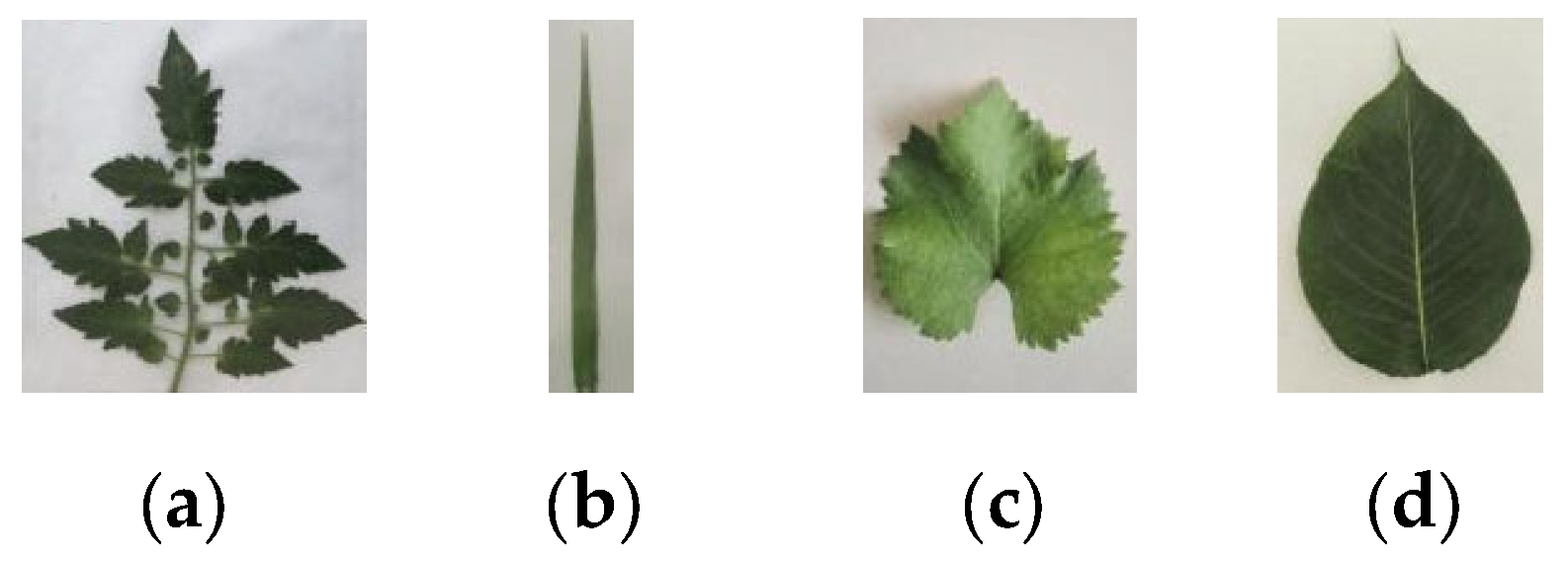
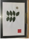
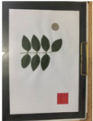
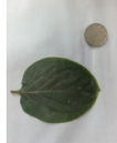
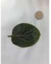
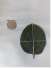
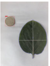
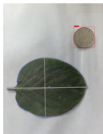
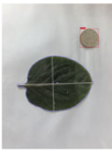
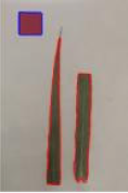
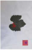
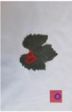
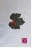
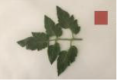
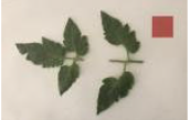
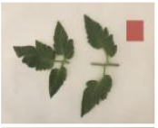
Leaf samples were collected from experimental fields at Shanxi Agricultural University (Taigu, Jinzhong, China), comprising green leaves of the same crop exhibiting varying shades due to environmental factors (light exposure duration, drought, pest/disease stress) as shown in Figure 1, along with morphologically diverse leaves from different crop species illustrated in Figure 2.

2.2. Method for Calculating Leaf Area

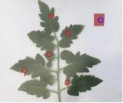
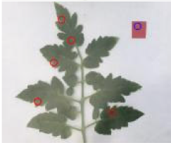
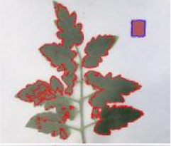
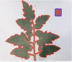
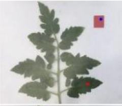
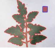
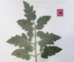
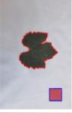
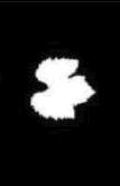
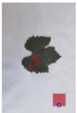
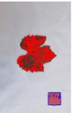
This system employs a reference marker-based approach for leaf area calculation, which involves positioning a reference marker of known area beside the target leaf. This method is consistent with techniques used in prior studies, such as Li Fangyi’s use of industrial-grade black frosted circular magnetic sheets (30 mm in diameter) to calculate the leaf area of individual rapeseed plants [9], and Guo Xiaojuan’s approach of utilizing a 1 cm black square for measuring wheat leaf area [13]. Figure 3 illustrates the integrated workflow for automated leaf area measurement. The process begins with image acquisition using a smartphone to capture pictures of a custom-designed leaf-bearing platform containing a leaf sample and a reference marker. Perspective distortion correction is then performed through Hough transform-based detection of the platform’s four interior edges, followed by a perspective transformation to rectify geometrical distortions. Prior knowledge is obtained by manually selecting 2–3 pixel points on both the leaf and reference regions in the rectified image, establishing adaptive thresholding which are then used to generate approximate contours through a thresholding method. The color image segmentation employs a probabilistic model that treats pixel colors as multivariate Gaussian distributions, formulating the segmentation as a Maximum A Posteriori (MAP) optimization problem with an energy function definition. By minimizing an energy functional using variational level set methods—auto-initialized from the approximate contours—the system achieves tri-class segmentation (leaf, reference, and background). Finally, the actual leaf area is calculated by scaling the pixel ratio between the leaf and reference regions, derived from level set evolution results, against the known physical area of the reference marker.

2.2.1. Image Acquisition

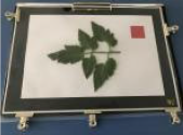
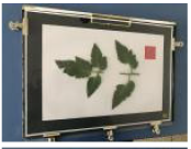
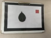
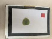
Image acquisition employs a custom-designed leaf-bearing platform featuring reference markers (Figure 4), comprising three components: a specimen mounting plate with black rectangular borders, a flexible transparent plastic cover, and a securing clip. The plate’s black borders facilitate perspective distortion correction through automated border detection, while its white rectangular substrate displays a pure red reference marker in the upper-right quadrant—exploiting red-green chromatic contrast to optimize color-based segmentation between predominantly green foliage and reference. Platform dimensions are scaled according to anticipated leaf sizes.

During image capture using digital cameras or smartphones, plant leaves must be evenly positioned within the central zone of the mounting plate under the following constraints: (1) free of foliar overlap, (2) contained entirely within the white detection area, (3) spatially isolated from the red reference marker, and (4) fully covered within the camera’s field of view. Resultant images must exhibit sharp focus without motion artifacts to ensure measurement validity.

2.2.2. Image Rectification

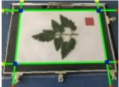
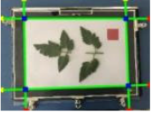
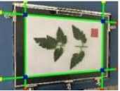
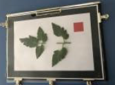
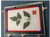
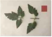
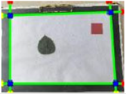
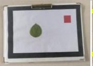
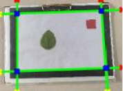
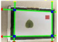
Variable camera height and imaging angle during capture introduce perspective distortion in acquired leaf images, compromising measurement accuracy. To mitigate this effect, our methodology implements a geometric rectification pipeline: (1) binarization and edge detection of raw images; (2) Hough transform-based localization of the four vertices defining the platform’s white detection area; (3) perspective transformation utilizing these vertices to correct spatial distortions, thereby enhancing area measurement precision.

1. Perspective Transformation

Perspective transformation, grounded in optical imaging principles, rectifies geometric distortions through computation of control points to derive a transformation matrix [3,14,15]. This technique fundamentally reprojects images onto a novel viewing plane, with its generalized transformation formula expressed as Equation (1):

$$\left[x^{\prime } y^{\prime } z^{\prime }\right]=\left[u v w\right] \cdot \mathrm{T}, \mathrm{T}= \left[\begin{array}{l}{a}_{11} a_{12 } a_{13}\\ a_{21} a_{22 } a_{23}\\ a_{31} a_{32 } a_{33}\end{array}\right],$$

(1)

where T denotes the perspective transformation matrix, ($u$,$v$) represent the original pixel coordinates, and $w=1$, and $a_{33}=1$. Defining the rectified pixel coordinates as ($x$,$y$) where $x=x\prime /z\prime$ and $y=y\prime /z\prime$, the perspective transformation equation is derived as Equation (2):

$$\left\{\begin{array}{l}x={\displaystyle \frac{x^{\prime }}{z^{\prime }}}={\displaystyle \frac{a_{11}u+a_{21}v+a_{31}}{a_{13}u+a_{23}v+a_{33}}}\\ y={\displaystyle \frac{y^{\prime }}{z^{\prime }}}={\displaystyle \frac{a_{12}u+a_{22}v+a_{32}}{a_{13}u+a_{23}v+a_{33}}}\end{array}\right.,$$

(2)

As evident from the derivation, four corresponding point pairs yield eight equations. Solving this system simultaneously determines the eight unknown parameters in transformation matrix T (excluding $a_{33}$). This computed matrix subsequently enables perspective warping of all pixel coordinates in the source image [14,15].

2. Hough Transform-Based Perspective Rectification

This work implements perspective correction through Hough transform-based line detection [16,17,18] and vertex computation, experimentally validating enhanced leaf area measurement accuracy. The workflow comprises four stages:

(1)

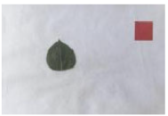
Preprocessing: Original images (Figure 5a) undergo binarization (Figure 5b) and edge detection (Figure 5c). Comparative evaluation of edge operators demonstrated the Laplacian of Gaussian (LoG) operator’s superior performance in extracting the platform’s rectangular contour.

(2)

Boundary Identification: Hough transform detects all line segments in Figure 5c, with the four longest lines corresponding to the platform’s borders (Figure 5d).

(3)

Geometric Registration:

a.

Source vertices: Intersection coordinates ($u_1,v_1$) to ($u_4,v_4$) from line equations.

b.

Target rectangle: Constructed using maximum horizontal/vertical spans with vertices ($x_1,y_1$) to $($x_4,y_4$).

(4)

Spatial Transformation:

a.

Perspective matrix derivation: Plugging source/target coordinates into Equation (2).

b.

Bicubic interpolation: Mitigates pixel loss during warping.

c.

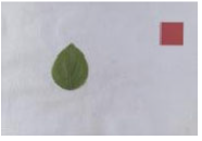
Background pruning: Extraneous regions beyond detection area removed (Figure 5e).

2.2.3. Color Image Segmentation

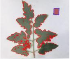
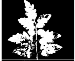
This study’s image segmentation aims to partition plant leaf, reference marker, and background into three disjoint regions, calculating actual leaf area through the pixel ratio between leaf and reference regions combined with the reference’s known physical area. We implement a region-based approach that models pixel colors via multivariate Gaussian distributions, formulates segmentation as a Maximum A Posteriori (MAP) optimization problem with an energy function definition, and minimizes this functional using variational level set method to derive curve evolution equations. This methodology fully leverages RGB color information while enabling direct segmentation visualization through level set evolution results and simultaneously extracting both leaf and reference markers.

1. Probabilistic Segmentation Model

This study models image color values as random variables with specific probability distributions, transforming image segmentation into a Maximum A Posteriori (MAP) optimization problem to construct a region-based statistical segmentation model.

Assuming the rectified image G is partitioned into three regions: leaf region M₁, reference marker region M₂, and background region M₃, we define M = {M₁, M_2, M₃}. Image segmentation is formulated as maximizing the posterior probability p(M|G) [19,20]. By Bayesian theory, assuming pixel-wise independence within each region, p(M|G) can be expressed as:

$$p(M|G)=p(\{M_i\}|G)={\displaystyle \frac{p(G|\{M_i\})}{p(G)}}p(\{M_i\})={\displaystyle \frac{{\displaystyle \prod _{s\in M_i}{p}_i(G(s))}}{p(G)}}p(\{M_i\}), i\in \{1,2,3\},$$

(3)

Since image G is given, p(G) remains constant. Defining p{M_i}) as the prior probability of pixels assigned to region M_i and assuming uniform priors (p{M_i} = 1/3), the maximum a posteriori (MAP) estimate simplifies to maximizing the likelihood term. Thus, ignoring constant and uniform factors, the energy functional E is defined as:

$$\begin{array}{l}E=\max (p(M|G))\\ =\max ({\displaystyle \prod _{s\in M_i}{p}_i(G(s))}) \\ =\max ({\displaystyle \prod _{s\in M_1}{p}_1(G(s))}{\displaystyle \prod _{s\in M_2}{p}_2(G(s))}{\displaystyle \prod _{s\in M_3}{p}_3(G(s))}) , i\in \{1,2,3\},\end{array}$$

(4)

To facilitate computation, we take the logarithm of the energy functional, transforming the above expression into:

$$\begin{array}{l}E =\max (\log ({\displaystyle \prod _{s\in M_1}{p}_1(G(s))}{\displaystyle \prod _{s\in M_2}{p}_2(G(s))}{\displaystyle \prod _{s\in M_3}{p}_3(G(s))}) )\\ =\max ({\displaystyle \sum _{s\in M_1}\log p_1(G(s))+{\displaystyle \sum _{s\in M_2}\log p_2(G(s))}}+{\displaystyle \sum _{s\in M_3}\log p_3(G(s))}) \\ =\max ({\displaystyle \sum _{i=1}^3{\displaystyle \sum _{M_i}\log p_i(G(s))}}) \\ =\max ({\displaystyle \sum _{i=1}^3{\displaystyle {\iint }_{M_i}\log p_i(G(s))}}), i\in \{1,2,3\}\end{array}$$

(5)

Here, p_i(G) denotes the probability density of a pixel value within region M_i, where each pixel contains three color components: red, green, and blue. To characterize color information and inter-channel correlations across the three regions, pixel values are assumed to follow a multivariate Gaussian distribution, whose probability density function is given by Equation (6):

$$p_i(G)={\displaystyle \frac{1}{{(2\pi )}^{d/2}|{\Sigma }_i{|}^{1/2}}}\exp (-{\displaystyle \frac{1}{2}}{(G-{\mu }_i)}^T{\Sigma }_i^{-1}(x-{\mu }_i)) i\in [1,2]$$

(6)

Here, μ_i and Σ_i denote the mean vector and covariance matrix for the i-th region, respectively, with d representing the data dimensionality. For RGB color images, d = 3.

The variational level set method seeks to minimize the energy functional. Consequently, we negate the functional defined in Equation (5), converting it to Equation (7):

$$\begin{array}{l}E =-{\displaystyle \sum _{i=1}^3{\displaystyle {\iint }_{M_i}\log (p_i(G))dxdy}}\\ =-{\displaystyle \sum _{i=1}^3{\displaystyle {\iint }_{M_i}\frac{1}{2}(G-{\mu }_i){\Sigma }_i^{-1}(G-{\mu }_i)-\frac{1}{2}\log |{\Sigma }_i|-\log {(2\pi )}^{d/2}dxdy}}\\ ={\displaystyle \sum _{i=1}^3{\displaystyle {\iint }_{M_i}\frac{1}{2}(G-{\mu }_i){\Sigma }_i^{-1}(G-{\mu }_i)+\frac{1}{2}\log |{\Sigma }_i|dxdy}}+{\displaystyle \sum _{i=1}^3{\displaystyle {\iint }_{M_i}\log {(2\pi )}^{d/2}dxdy}}\end{array}$$

(7)

Multiplying Equation (7) by 2 and discarding constant terms preserves the optimization solution. Thus, Equation (7) is reformulated as:

$$E ={\displaystyle \sum _{i=1}^3{\displaystyle {\iint }_{M_i}(G-{\mu }_i){\Sigma }_i^{-1}(G-{\mu }_i)+\log |{\Sigma }_i|dxdy}}$$

(8)

2. Level Set Curve Evolution Implementation

This work minimizes the energy functional in Equation (8) by leveraging variational level set curve evolution [21,22,23,24,25,26,27]. The implementation comprises: (1) representing image regions through level set functions, and (2) deriving the curve evolution equation via variational calculus. This drives the level set function along the steepest energy descent gradient, ultimately yielding planar closed curves that partition the image into non-overlapping regions.

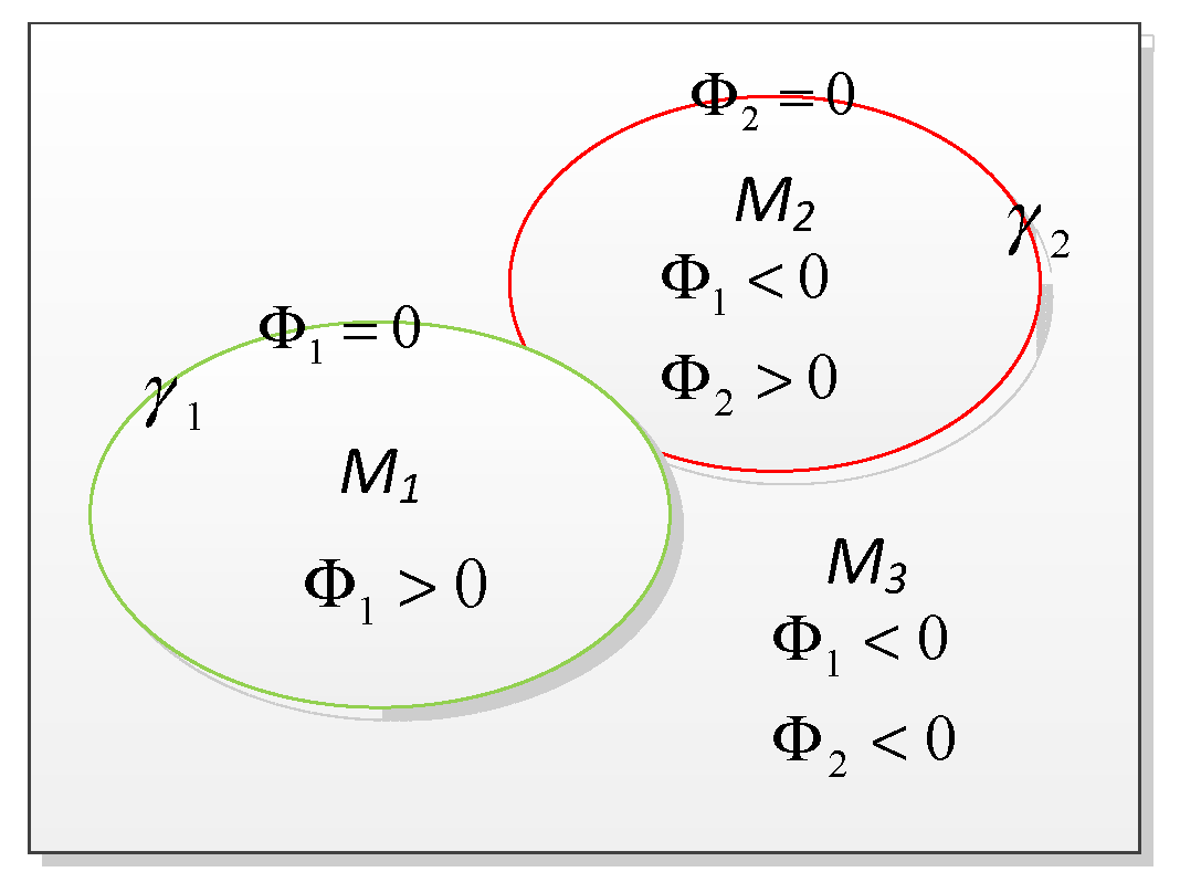
Level Set Representation of Image Regions: Let Ω denote the image domain. Two level set functions ${\mathsf{\Phi }}_1$ and ${\mathsf{\Phi }}_2$ define three mutually exclusive regions:

$$\begin{gathered} \mathrm{Leaf} \mathrm{region} M_1: M_1=M_{\mathsf{\Phi }1} \\ \mathrm{Reference} \mathrm{region} M_2: M_2=M_{\mathsf{\Phi }1}^C\cap M_{\mathsf{\Phi }2} \\ \mathrm{Background} \mathrm{region} M_3: M_3=M_{\mathsf{\Phi }1}^C\cap M_{\mathsf{\Phi }2}^C \end{gathered}$$

where the planar curve ${\gamma }_i=\{x\in \mathsf{\Omega }|{\mathsf{\Phi }}_i\left(x\right)=0,i\in \mathrm{1,2}\}$ bounds region $M_{\mathsf{\Phi }i}$ (interior: ${\left\{x\in \mathsf{\Omega }\right| \mathsf{\Phi }}_i\left(x\right)>0\}$) and $M_{\mathsf{\Phi }i}^C$ (exterior: $\{x\in \mathsf{\Omega }|{\mathsf{\Phi }}_i\left(x\right)<0\}$). Figure 6 illustrates this regional partitioning scheme.

Thus, Equation (8) can be expressed in terms of level set functions as:

$$E={\displaystyle {\iint }_{M_{\Phi 1}}{e}_1}dxdy+{\displaystyle {\iint }_{M_{\Phi 1}^C\cap M_{\Phi 2}}{e}_2}dxdy+{\displaystyle {\iint }_{M_{\Phi 1}^C\cap M_{\Phi 2}^C}{e}_3}dxdy$$

(9)

where $e_i=(G-{\mu }_i){\Sigma }_i^{-1}(G-{\mu }_i)+\log |{\Sigma }_i|$.

To obtain smooth contour evolution, we incorporate the regularization term from the Chan-Vese (C-V) model [21], reformulating Equation (10) as Equation (10):

$$E={\displaystyle {\iint }_{M_{\Phi 1}}{e}_1}dxdy+{\displaystyle {\iint }_{M_{\Phi 1}^C\cap M_{\Phi 2}}{e}_2}dxdy+{\displaystyle {\iint }_{M_{\Phi 1}^C\cap M_{\Phi 2}^C}{e}_3}dxdy+\lambda {\displaystyle \sum _{i=1}^2{\displaystyle {\oint }_{{\gamma }_i}ds}}$$

(10)

Applying shape derivative calculus [28] to Equation (9) yields the curve evolution equation through partial differentiation:

$$\left\{\begin{array}{l}{\displaystyle \frac{\partial {\Phi }_1}{\partial t}}=-(e_1-e_2{\chi }_{\{{\Phi }_2>0\}}-e_3{\chi }_{\{\Phi 2\le 0\}}+\lambda K_1)||\overrightarrow{\nabla }{\Phi }_1||\\ {\displaystyle \frac{\partial {\Phi }_2}{\partial t}}=-({\chi }_{\{{\Phi }_1\le 0\}}(e_2-e_3)+\lambda K_2)||\overrightarrow{\nabla }{\Phi }_2||\end{array}\right.$$

(11)

where $\chi ({\Phi }_i\le 0)=\left\{\begin{array}{l}1 {\Phi }_i\le 0\\ 0 {\Phi }_i>0\end{array}\right.$, $\chi ({\Phi }_i>0)=\left\{\begin{array}{l}1 {\Phi }_i>0\\ 0 {\Phi }_i\le 0\end{array}\right.$, $K_i=\nabla \cdot {\displaystyle \frac{\nabla {\Phi }_i}{|\nabla {\Phi }_i|}}$, $i\in \{1,2\}$ Experiments confirm that the curve evolution Equation (11) achieves excellent convergence and high precision, but exhibits slow computational efficiency. To enhance evolution speed, we refine this formulation by incorporating the Heaviside function and Dirac function defined in Equation (12).

$$H(z)=\left\{\begin{array}{l}1 z\ge 0\\ 0 z<0\end{array}\right., \delta (z)={\displaystyle \frac{d}{dz}}H(z)$$

(12)

Furthermore, to simultaneously streamline level set initialization and eliminate re-initialization during evolution, we integrate the internal penalty energy $P(\Phi )={\displaystyle {\iint }_{\Omega }\frac{1}{2}{(\nabla \Phi -1)}^{2}dxdy}$ proposed by Chunming Li [29]. This dual-purpose approach accelerates curve evolution and enables φ₀ to be initialized as follows:

$${\Phi }_0=\left\{\begin{array}{l}d (x,y) \mathrm{inside} \mathrm{the} \mathrm{plane} \mathrm{curve} {\gamma }_i\\ 0 (x,y) \mathrm{on} \mathrm{the} \mathrm{plane} \mathrm{curve} {\gamma }_i\\ -d (x,y) \mathrm{outside} \mathrm{the} \mathrm{plane} \mathrm{curve} {\gamma }_i \end{array}\right.$$

(13)

Therefore, Equation (10) can be expressed by heavside function and Dirac function as:

$$\begin{array}{l}E={\displaystyle {\iint }_{\Omega }{e}_{1}H({\Phi }_1)dxdy}+{\displaystyle {\iint }_{\Omega }{e}_2(1-H({\Phi }_1))H({\Phi }_2)dxdy} \\ +{\displaystyle {\iint }_{\Omega }{e}_3(1-H({\Phi }_1))(1-H({\Phi }_2))dxdy} \\ +\lambda \cdot {\displaystyle \sum _{i=1}^2{\displaystyle {\iint }_{\Omega }|\nabla H({\Phi }_i)|dxdy}}+\mu \cdot {\displaystyle \sum _{i=1}^2{\displaystyle {\iint }_{\Omega }\frac{1}{2}{(|\nabla {\Phi }_i|-1)}^{2}dxdy}}\end{array}$$

(14)

Applying variational calculus [23] to the above formulation, we derive its Euler–Lagrange equation, yielding the evolution equation shown in Equation (15):

$$\left\{\begin{array}{l}{\displaystyle \frac{\partial {\Phi }_1}{\partial t}}=-\delta ({\Phi }_1)\cdot (e_1-e_2\cdot H({\Phi }_2)-e_3\cdot (1-H({\Phi }_2)) +\lambda K_1)+\mu (\Delta {\Phi }_1-K1)\\ {\displaystyle \frac{\partial {\Phi }_2}{\partial t}}=-\delta ({\Phi }_2)\cdot ((1-H({\Phi }_1))\cdot (e_2-e_3)+\lambda K_2)+\mu (\Delta {\Phi }_2-K2)\end{array}\right.$$

(15)

where $\mathsf{\Delta }$ is Laplacian operator.

Empirical analysis confirms that the evolution equation (Equation (11)) delivers robust convergence and high segmentation accuracy but exhibits slow computational performance. In contrast, Equation (15) achieves accelerated evolution yet suffers from unstable convergence and diminished precision. To resolve this accuracy–speed tradeoff, we implement an integrative framework combining both equations, enhancing computational efficiency while maintaining segmentation fidelity.

2.2.4. Algorithm Description and System Development

1. Algorithm Description

The leaf area calculation algorithm presented in this study comprises the following steps:

(1)

Image Rectification: Acquired images undergo rectification using the method detailed in Section 2.2.2, yielding rectified images. Rectification can be performed either manually or automatically.

(2)

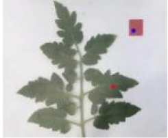
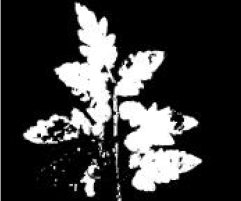
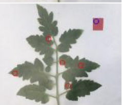
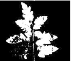
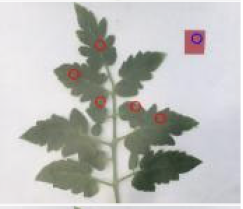
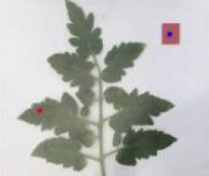
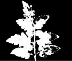
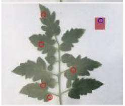
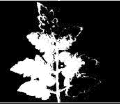
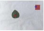
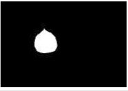
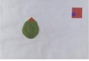
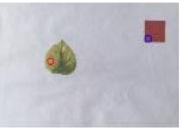
Adaptive Thresholding and Rough Segmentation: On the rectified image, manually select n₁ sample points on the leaf and n₂ points on the reference object to obtain two sets of adaptive thresholds. The RGB color values acquired from these samples are converted to the HSV color space. The minimum and maximum hue (H) values from all sampled points are then calculated to define the hue range of the leaf. This hue range is used as a threshold to segment the approximate regions of the leaf and the reference object, thereby providing a foundation for the automatic initialization of the level set initial contour.

(3)

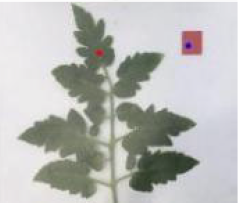
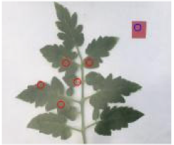
Initial Contour Definition: Within the segmented rough regions, automatically and randomly define multiple small circles as initial contours using Equation (13) (where d is the function value). Parameters include scaling factor p, circle radius r, number of initial leaf contours c₁, and number of initial reference object contours c₂.

(4)

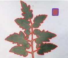
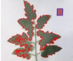
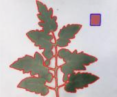
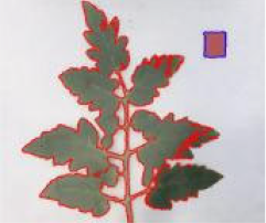
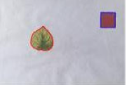
Curve Evolution: Perform curve evolution for iter₁ iterations according to Equation (15), followed by iter₂ iterations according to Equation (11) (total iterations iter = iter₁ + iter₂). This process converges with the final contours of the leaf and reference object.

(5)

Area Calculation: Extract the final contours to determine the number of pixels within the leaf region (N_leaf) and the reference object region (N_ref). Given the known true area of the reference object (A_ref), the true leaf area (A_leaf) is calculated as [30]:

$$\mathrm{A}\_\mathrm{leaf}={\displaystyle \frac{\mathrm{N}\_\mathrm{leaf}}{\mathrm{N}\_\mathrm{ref}}}\times \mathrm{A}\_\mathrm{ref}$$

(16)

2. System Development

(1)

Computational Environment

All subsequent processing and analysis were performed on a laptop computer running Windows 11. The development platform was MATLAB R2023b. The hardware configuration included an AMD Ryzen 9 6900HX CPU, 32 GB of RAM, and an NVIDIA GeForce RTX 3060 Laptop GPU.App Development.

(2)

Imaging Setup

The sample images were captured using a Huawei P40 Pro smartphone camera manufactured by Huawei Technologies Co., Ltd. in Shenzhen, China. Our methodology is specifically designed to be robust to varying shooting distances and angles through perspective correction. Therefore, the shooting height and angle were unconstrained, but the phone was positioned as close to the subject as possible to fulfill two criteria: (1) to include the entire leaf platform within the field of view, and (2) to ensure high-resolution image quality capable of revealing fine edge details of the leaves.

(3)

App Development

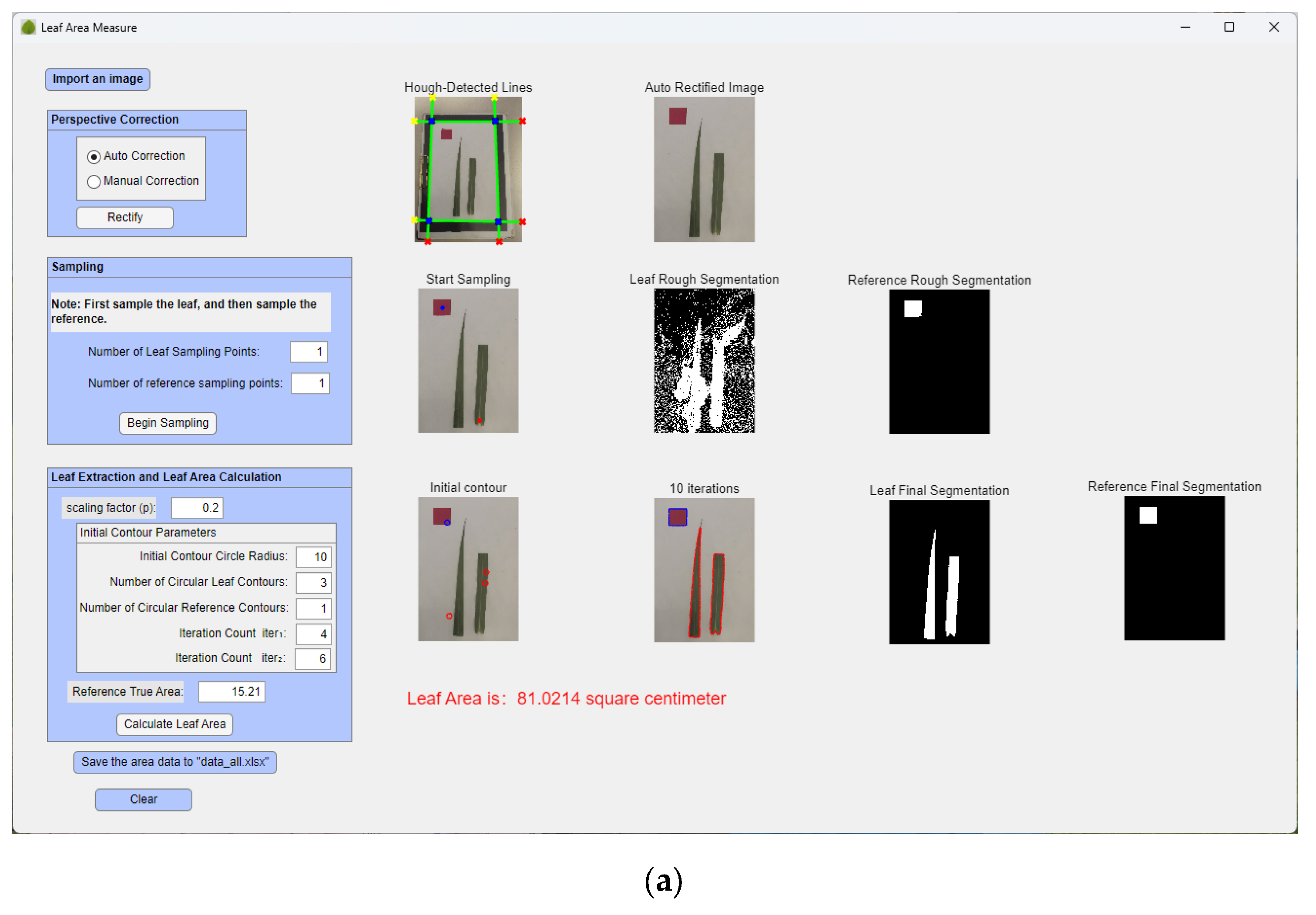
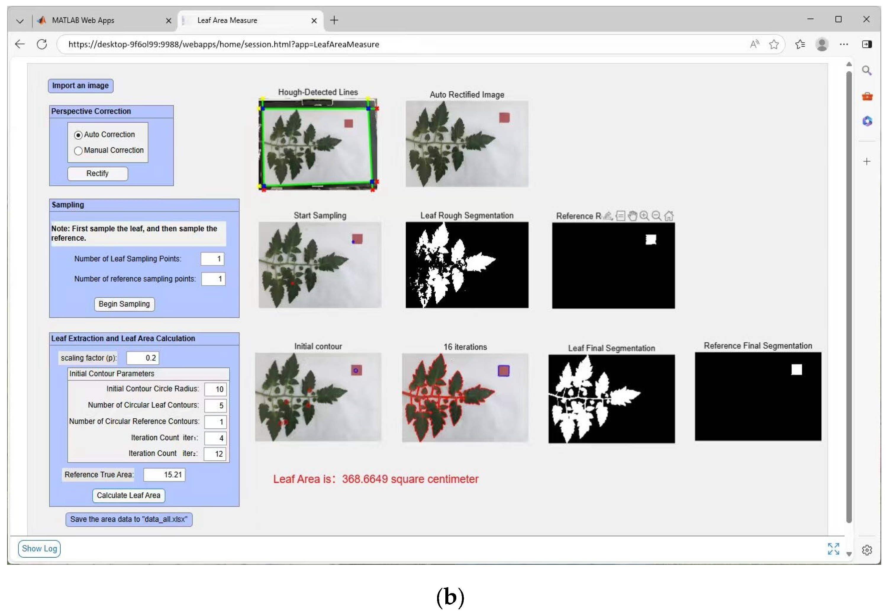
To enhance operational efficiency and practicality, the system provides two deployment options: a standalone EXE application Version 1.0 and a Web-based application Version 1.0. The EXE version requires local installation but operates independently of internet connectivity, making it suitable for environments with limited or unstable network access. However, it consumes more storage space compared to the web version. The web application, accessible via a browser without installation, offers greater accessibility and convenience for multi-user scenarios but relies on server availability and maintenance.

As shown in Figure 7a, the EXE interface enables full parameter customization—including sampling point quantity, initial contour circle settings, image scaling ratio, and iteration counts—within a localized environment. Meanwhile, Figure 7b illustrates the web interface, which provides similar functionality through a browser-based platform. In both versions, the initial contour circles are automatically generated by the algorithm, ensuring consistency and objectivity in the initialization process.

3. Results

To validate the practicality and measurement accuracy of our leaf area extraction algorithm, we designed two complementary experiments. The first experiment evaluated image rectification functionality using geometrically congruent paper specimens with contrasting colors. The second experiment assessed algorithmic performance across diverse crop species by comparing leaf area measurements derived from our method under multiple parameter configurations against ground-truth values obtained via manual photocopy-weighing technique. This comparison encompassed leaves exhibiting substantial variations in morphology and coloration.

To ensure the conciseness and readability of the tables, this study adopts the following measures. First, a summary of evaluation metrics and their mathematical definitions is provided in

Table A1. Formulas and Variable Descriptions for Key Statistical Metrics.

Metric (Abbreviation)	Formula	Variable Definitions
AE	$\mathrm{AE}=|y-\widehat{y}|$	$y$$\widehat{y}$: measured value
RE	$\mathrm{RE}={\displaystyle \frac{|y-\widehat{y}|}{y}}$
SD	$\mathrm{SD}=\sigma =\sqrt{{\displaystyle \frac{{\displaystyle \sum _{i=1}^n{(x_i-\mu )}^2}}{n-1}}}$$, \mu ={\displaystyle \frac{{\displaystyle \sum _{i=1}^n{x}_i}}{n}}$	$n$: total number of samples $x_i$: the i-th sample value $\mu$: sample mean
CV	$\mathrm{CV}={\displaystyle \frac{\sigma }{\mu }}\times 100\%$,
RMSE	$\mathrm{RMSE}=\sqrt{{\displaystyle \frac{{\displaystyle \sum _{i=1}^n{(y_i-{\widehat{y}}_i)}^2}}{n}}}$	$y_i$: the i-th true value ${\widehat{y}}_i$: the i-th measured or predicted value $n$: total number of samples
R2	${\mathrm{R}}^2=1-{\displaystyle \frac{s{s}_{res}}{s{s}_{tot}}}$$, s{s}_{res}={\displaystyle \sum _{i=1}^n{(y_i-{\widehat{y}}_i)}^2}$$, s{s}_{tot}={\displaystyle \sum _{i=1}^n{(y_i-\overline{y})}^2}$$, \overline{y}={\displaystyle \frac{{\displaystyle \sum _{i=1}^n{y}_i}}{n}}$

(Appendix A); see the Abbreviations list for acronyms of the metrics. Second, standardized abbreviations are employed consistently across the Results and Discussion section.

Table 1. Glossary of Abbreviations Used in the Study.

Abbreviation	Full Term	Abbreviation	Full Term
Orig.	Original	Fin.	Final
Rect.	Rectified	Meas.	Measured
Ref.	Reference	Prop.	Proposed Method
Seg.	Segmentation	OP.	OpenPheno
Auto-Init.	Auto-Initialized	IJ.	ImageJ
Cont.	Contours	Sh.	Shooting
Evol.	Evolution	H1–H4	Height 1–Height 4

lists these abbreviations alongside their full terms for clarity and reference. These primarily encompass key concepts in image processing terminology, measurement parameters, and method names.

3.1. Image Rectification Functionality Validation

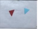
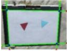
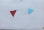
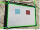
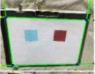
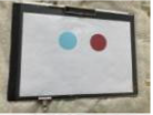
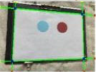
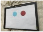
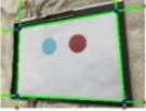
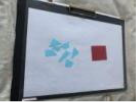
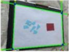
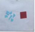
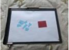
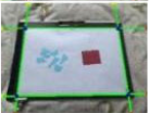
Under controlled laboratory conditions, geometrically congruent red and blue paper specimens were positioned on our reference-free Leaf Platform. Images were acquired from multiple perspectives to induce perspective distortions. The proposed method extracted specimen areas, computing red-to-blue area ratios. Ten replicate measurements for unrectified/rectified states were averaged per condition. Table 1 presents representative pre-/post-rectification ratios for diverse geometries (triangles, quadrilaterals, circles, irregular quadrilaterals).

As evidenced in

Table 2. Pre-/Post-Rectification Area Ratios.

Orig. Image	Hough Lines	Rect. Image	Ref. Ratio	Ratio (Pre)	Ratio (Post)	RE (Pre) (%)	RE (Post) (%)
			1	1.3197	1.0008	31.97	0.08
			1	1.0931	0.9923	9.31	0.77
			1	0.7118	0.9949	28.82	0.51
			1	0.9107	1.0016	8.93	0.16
			1	0.8593	1.0027	14.07	0.27
			1	1.2966	0.9976	29.66	0.24
			1	0.6668	1.0091	33.32	0.91
			1	0.9309	0.9915	6.91	0.85

, unrectified specimens exhibited substantial relative errors (RE) in area ratios (up to 33.32%). Post-rectification ratios consistently approached 1.0 with RE below 1%, confirming the effectiveness of our perspective rectification method in meeting agricultural measurement precision requirements.

3.2. Leaf Extraction Workflows for Diverse Crop Species

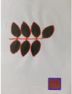
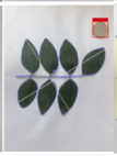
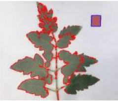
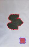
The proposed method extracted leaves from diverse crop species (Figure 1 and Figure 2) exhibiting distinct morphological and chromatic characteristics: tomato leaves with complex marginal structures, grape leaves featuring serrated edges, pear leaves showing variegated pigmentation, and broomcorn millet leaves demonstrating simple, smooth margins. Representative extraction workflows are documented in

Table 3. Leaf Extraction Workflows for Diverse Crop Species.

Orig. Image	Hough Lines	Manual Seeds	Rough Seg. (leaf)	Rough Seg. (Ref.)	Auto-Init. Cont.	Evol. Stage	Fin. Cont.	Leaf Fin. Seg.	Ref. Fin. Seg.

.

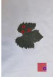
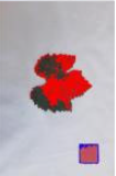
Table 3 demonstrates robust segmentation performance across diverse crops and leaf morphologies. The method successfully extracts both individual and clustered leaves (Row 6) while generating precise leaf and reference object contours (Column 8), enabling visual quality assessment. Key parameter adaptation principles include:

(1)

Size-dependent scaling: Increase initial circle radius, count, and iterations for larger leaves; decrease for smaller specimens.

(2)

Over-segmentation compensation: Elevate circle count when rough segmentation exceeds target boundaries to ensure adequate on-leaf initialization.

(3)

Algorithmic resilience: Randomized circle placement achieves accurate contours even with suboptimal initialization (e.g., broomcorn millet, Row 5: 2/5 circles overlapping leaf).

3.3. Comprehensive Leaf Area Measurements Across Crops and Parameters

Table 4. Comprehensive leaf area measurements.

Leaf Type	GT 1 Mean Area (cm2)	Meas. Mean Area (cm2)	SD (cm2)	CV (%)	RMSE (cm2)	AE (cm2)	RE (%)	Min Meas. Time (s)
Pear_1	54.32	53.91	0.98	1.82	1.82	0.41	0.75	5.23
Pear_2	79.34	79.00	0.98	1.06	1.24	0.34	0.43	5.28
Pear_3	37.18	36.84	0.90	2.44	0.96	0.34	0.91	3.40
Pear_4	26.65	26.91	0.55	2.04	0.95	0.26	0.98	3.36
Pear_5	43.03	43.24	0.94	2.18	0.96	0.21	0.49	5.93
Tomato_1	37.71	37.34	0.69	1.84	0.783	0.37	0.98	5.24
Tomato_2	77.31	77.83	0.98	1.26	1.108	0.52	0.67	4.54
Tomato_3	91.09	90.19	0.97	1.08	1.322	0.9	0.99	5.39
Tomato_4	96.42	96.40	0.99	1.03	0.991	0.02	0.02	7.47
Tomato_5	112.18	111.68	0.97	0.87	1.094	0.5	0.45	8.12
Tomato_6	136.70	137.07	1.94	1.42	1.97	0.37	0.27	9.05
B_millet_1	19.36	19.47	0.54	2.77	0.549	0.11	0.57	3.86
B_millet_2	31.43	31.41	0.90	2.86	0.896	0.02	0.06	6.80
B_millet_3	33.10	33.29	0.72	2.16	0.74	0.19	0.57	4.62
B_millet_4	34.56	34.85	0.71	2.05	0.768	0.29	0.84	6.98
B_millet_5	70.59	70.78	0.96	1.36	0.976	0.19	0.27	5.74
Grape_1	60.77	60.28	0.94	1.56	1.06	0.49	0.81	5.11
Grape_2	71.58	71.17	1.00	1.40	1.074	0.41	0.57	5.65
Grape_3	88.12	88.16	0.97	1.3	1.103	0.04	0.05	4.54
Grape_4	91.31	90.91	0.98	1.44	1.077	0.4	0.44	5.23
Grape_5	112.18	111.22	0.94	0.85	1.339	0.96	0.86	5.21

¹ GT = Ground Truth, obtained via manual photocopy-weighing technique.

presents comprehensive leaf area measurements for pear, tomato, broomcorn millet and grape under varying parameters (imaging angles and heights, sampling points, initial contours, iterations). Results include mean area (derived from ≥100 repetitions; the specific data sources and measurement repetitions for each crop are detailed in

Table 5. Data Sources under different shooting angles and heights and Measurement Repetitions for Table 3.

Leaf Type	Repetitions	Sh. 1	Sh. 2	Sh. 3	Sh. 4	Sh. 5	Sh. 6	Sh. 7	Sh. 8	Sh. 9	Sh. 10	Sh. 11	Sh. 12
Pear_1	110
Pear_2	113
Pear_3	195
Pear_4	177
Pear_5	107
Tomato_1	116
Tomato_2	156
Tomato_3	106
Tomato_4	222
Tomato_5	200
Tomato_6	313
B_millet_1	143
B_millet_2	151
B_millet_3	164
B_millet_4	174
B_millet_5	221
Grape_1	282
Grape_2	294
Grape_3	229
Grape_4	236
Grape_5	371

), standard deviation (SD), coefficient of variation (CV), and errors relative to photocopy-weighing (root mean square error RMSE, relative error RE; 10 weighing repetitions). The method demonstrates exceptional stability (SD < 1 cm²) and precision (RMSE < 2 cm²) for most images, though tomato and grape exhibit marginally higher RMSE than millet due to error amplification from complex margins in the photocopy-weighing method. Most measurements satisfy strict accuracy thresholds: absolute error (AE) < 1 cm², CV < 3%, RE < 1%. Computational efficiency is evidenced by minimum measurement times < 10 s per leaf—representing substantial efficiency gains over manual techniques. Owing to space constraints, only a subset of the measurement data for Pear_5 under different imaging angles, heights, and parameters is presented in

Table 6. Summary of Partial Measurement Data for Pear_5 under Various Imaging Parameters.

Shooting Name	Meas. Leaf Area (cm2)		Meas. Time (s)	Scaling Factor (p)		iter1	iter2	c1	c2	r
Sh. 1	44.3877		6.0915	0.2		1	3	3	1	10
Sh. 1	44.4377		8.6088	0.2		1	5	1	1	10
Sh. 1	44.7547		8.3736	0.2		1	5	3	1	10
Sh. 1	44.6804		6.6870	0.1		2	4	2	1	5
Sh. 1	44.8210		9.3218	0.2		2	4	3	1	10
Sh. 2	42.0385		9.1475	0.2		1	5	1	1	10
Sh. 2	42.1926		8.9257	0.2		1	5	3	1	10
Sh. 2	42.8226		11.5620	0.2		1	7	1	1	10
Sh. 2	42.4920		9.5679	0.2		2	4	3	1	10
Sh. 2	42.2359		15.0976	0.2		2	6	3	1	10
Sh. 3	42.1047		12.1156	0.2		1	5	1	1	10
Sh. 3	42.5355		12.8461	0.2		2	4	1	1	10
Sh. 3	43.8534		28.6916	0.3		2	4	2	1	15
Sh. 3	43.4826		7.3114	0.1		2	4	2	2	5
Sh. 3	43.5182		8.4654	0.1		2	6	2	1	5
Sh. 4	43.9285		8.4622	0.2		2	4	2	1	10
Sh. 4	43.6243		8.5215	0.2		2	4	2	1	10
Sh. 4	43.6756		8.6725	0.2		2	4	2	1	10
Sh. 4	43.9184		8.8893	0.2		2	4	2	1	10
Sh. 4	42.5147		9.1388	0.2		2	4	2	1	10
Sh. 5	43.7698		5.9310	0.1		2	4	2	1	5
Sh. 5	43.8995		6.0577	0.1		2	4	2	1	5
Sh. 5	43.9360		6.4218	0.1		2	4	2	1	5
Sh. 5	44.5514		6.4735	0.1		2	4	2	1	5
Sh. 5	43.7880		6.6547	0.1		2	4	2	1	5
Mean Area (cm2)		43.5185			RMSE (cm2)			1.0053
SD (cm2)		0.8963			CV (%)			2.06
GT Area (cm2)		43.0292			Min Measured Time(s)			5.9310

, along with its statistical summary.

3.4. Comparison with OpenPheno and ImageJ

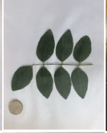
OpenPheno is an open-access, user-friendly, and smartphone-based platform designed for instant plant phenotyping [31]. Implemented as a WeChat Mini Program, it supports rapid plant trait analysis directly on mobile devices. In this study, leaf area was measured using both OpenPheno and ImageJ—a widely adopted image processing tool—and their performance was compared against the proposed method.

During the experiment, each leaf was placed on the platform described in Section 2.2.1 and remained fixed throughout the process. First, leaf area was measured with the proposed method using images captured via a smartphone. A one-yuan coin was then placed beside the leaf following OpenPheno’s scale calibration protocol, and another image was acquired for analysis with both OpenPheno and ImageJ. Comparative results of the three methods are summarized in

Table 7. Comparison of Leaf Area Measurement Results Across Different Methods and Conditions.

Description	Multi-Branch Leaf			Single-Branch Leaf			ImageJ: Different References				OpenPheno: Different Heights
	Prop.	OP.	IJ.	Prop.	OP.	IJ.	Coin		Rectangle		H11	H2	H3	H4
Original Image
Leaf Extraction
Local Zoom
Leaf Area (cm2)	86.25	82.82	84.76	54.75	49.69	52.04	87.78	85.88	89.48	91.60	53.29	52.59	47.68	51.24

.

The results indicate that all three methods successfully extracted leaf area on single-branch leaves. However, OpenPheno exhibited occasional inaccuracies in segmenting multi-branch leaves, as shown in the three column of Table 6. Measured leaf areas varied across methods.

OpenPheno yielded inconsistent results when applied to images of the same leaf captured at different heights. While it offers fully automated measurement without parameter adjustment—promoting reproducibility under consistent conditions—it lacks the flexibility for parameter tuning when extraction errors are visually detected.

ImageJ also showed variability in measured area when different reference objects were used within the same image. This inconsistency stems from its reliance on manual operations, including scale calibration, threshold adjustment, and/or manual leaf outlining. As a result, measurement accuracy is highly user-dependent, and reproducibility is limited.

In contrast, the proposed method employs a semi-automatic workflow. Although not fully automated, it allows parameter adjustment when erroneous extraction is identified, facilitating accurate leaf area measurement. This approach strikes a balance between automation and manual intervention, delivering robust and accurate results through simple and intuitive parameter settings.

4. Discussion

4.1. Impact of Manual Sampling Points

Manual sampling point selection is sensitive to lighting and viewing angle variations, generating notably different rough segmentation regions—especially for leaves—as documented in

Table 8. Experimental Results for Different Manual Sampling Points on Identical Rectified Image.

Manual Seeds	Rough Seg. (Leaf)	Auto-Init. Cont.	Evol. Stage	Fin. Cont.	Meas. Area (cm2)	Meas. Time (s)
					445.21	25.64
					446.12	24.66
					446.01	24.67
					444.17	23.91
					446.49	23.31
					445.91	25.33

. While these variations affect level set initialization contours, our method demonstrates remarkable consistency: under heterogeneous illumination, divergent sampling points yield different initial regions but ultimately produce equivalent leaf areas (SD = 0.8376 cm²) and comparable processing times (SD = 0.8674 s). With both standard deviations below 1.0, results confirm method robustness against sampling point variability.

4.2. Impact of Initial Contour Configuration

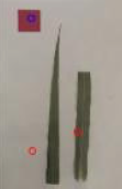
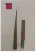
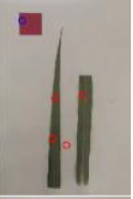
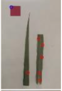
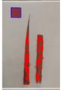
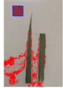
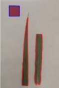
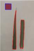
A broomcorn millet case study (rough segmentation regions shown in Figure 8) examined stochastic initial contour effects by varying target contour count (c₁) under fixed parameters (p = 0.2, r = 50p, iter₁ = 4, iter₂ = 6, c₂ = 1). As

Table 9. Extraction Results of Broomcorn Millet Under Different number of Initial Leaf Contour Configurations.

Parameter/Metric	c1 = 1	c1 = 1	c1 = 2	c1 = 2	c1 = 3	c1 = 4	c1 = 6	c1 = 10
Auto-Init. Cont.
Iter = 2
Iter = 10
Meas. area (cm2)	71.87	81.17	81.54	81.14	80.58	82.16	81.09	81.99
Meas. Time (s)	20.73	21.10	19.18	20.33	18.08	19.03	18.35	18.42

demonstrates: (1) At c₁ = 1, segmentation success depended stochastically on circle-leaf overlap (Column 2: success; Column 1: failure); (2) For c₁ ≥ 2, correct segmentation occurred consistently despite partial coverage (Columns 4–6). Method robustness was confirmed through minimal outcome variation (leaf area SD = 0.5526 cm²; processing time SD = 0.8740 s; both <1.0), validating reliability across contour initialization scenarios.

4.3. Impact of Scaling Factor Variation

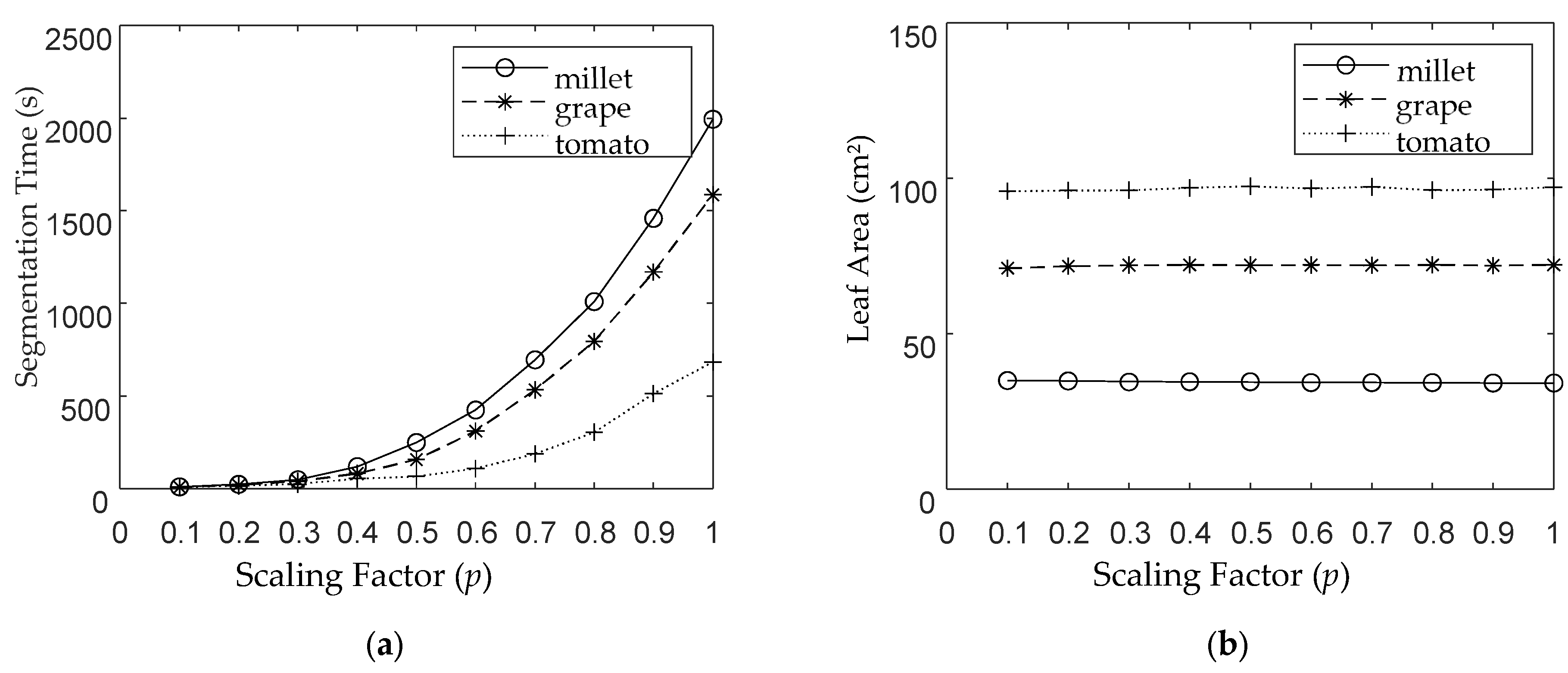
To evaluate scaling factor (p) effects, rectified images of broomcorn millet (3507 × 2358 px; smooth margins), grape (2518 × 3715 px; serrated margins), and tomato (1969 × 2879 px; serrated and lobed) were analyzed under fixed parameters (r = 50p, c₁ = 3, c₂ = 1, iter₁ = 4, iter₂ = 6) with all metrics averaged over 10 repetitions. As demonstrated in Figure 9a and

Table 10. Mean Leaf Area (cm²) and Segmentation Time (s) Across Scaling Factors (Values averaged over 10 repetitions).

Species/Morphology	Parameter	Scaling Factor (p)
		0.1	0.2	0.3	0.4	0.5	0.6	0.7	0.8	0.9	1
Broomcorn millet (Smooth margins)	Area	34.97	34.82	34.50	34.60	34.56	34.24	34.31	34.29	34.19	34.12
	Time	9.58	22.61	49.51	120.12	248.08	425.27	695.68	1010.94	1458.95	1995.62
Grape (Serrated-only margins)	Area	71.09	71.78	72.09	72.19	72.13	72.13	72.05	72.21	71.95	72.20
	Time	9.22	19.14	40.43	81.93	157.62	310.65	533.57	796.52	1169.33	1586.34
Tomato (Serrated + Lobed)	Area	95.83	96.09	96.15	96.95	97.45	96.71	97.26	96.17	96.37	97.15
	Time	8.35	15.59	24.65	55.02	66.07	109.23	188.29	304.56	513.01	684

, segmentation time scales near-exponentially with p (Coefficients of Determination R² > 0.99) and correlates with image dimensions rather than biological leaf area—evidenced by 65.7% faster tomato processing (684 s vs. 1995.62 s at p = 1) despite its 180% larger leaf area (96.61 cm² vs. 34.46 cm²). Crucially, leaf area measurements exhibit exceptional stability across scaling factors (Figure 9b), with all standard deviations <1 cm² (max SD = 0.57 cm² for tomato) and coefficients of variation <1% (

Table 11. Statistical Analysis of Measurement Stability.

Metric	Broomcorn Millet (Smooth)	Grape (Serrated)	Tomato (Serrated + Lobed)
MaxΔArea 1 (cm2)	0.85	1.12	1.62
SD (cm2)	0.28	0.34	0.57
CV (%)	0.81	0.47	0.59
GT Area (cm2)	34.56	71.58	96.42
RMSE (cm2)	0.28	0.52	0.57
Time Model R2	0.9909	0.9894	0.9915

¹ Max_ΔArea = Max Area Difference.

). Observed RMSE variations (0.28–0.57 cm²) primarily reflect reference method limitations: minimal error for smooth-margined millet (0.28 cm²), moderate for serrated-only grape (0.52 cm²), and maximal for serrated and lobed tomato (0.57 cm²), confirming the algorithm’s scaling-invariant precision while attributing discrepancies to manual measurement challenges with complex morphologies.

4.4. Impact of Iteration Counts

This study examines the impact of iteration counts iter₁ and iter₂ on segmenting grape leaf images using fixed parameters (p = 0.2, r = 50p, c₁ = 3, c₂ = 1). As summarized in

Table 12. Experimental results under different iteration counts.

Iteration Counts	Auto-Init. Cont.	iter = iter1 + iter2									Leaf Fin. Seg.	Meas. Area (cm2)	Meas. Time (s)
		2	4	6	10	20	40	60	80	100
iter1 = 0 iter2 = 100												91.41	143.17
iter1 = 100 iter2 = 0												86.67	136.58
Iter1 = 80 Iter2 = 20												91.32	127.07

, when only Equation (11) was applied (e.g., iter₁ = 0, iter₂ = 100), curve evolution was slow yet stable, requiring 80 iterations to approximate the leaf contour but yielding a leaf area consistent with manual measurements. Using only Equation (15) (e.g., iter₁ = 100, iter₂ = 0) accelerated initial contour detection achieving a rough outline within 10 iterations, but at the cost of reduced smoothness and increased area error due to poor convergence. A hybrid approach (e.g., iter₁ = 80, iter₂ = 20) balanced speed and accuracy, delivering a well-converged contour with higher precision.

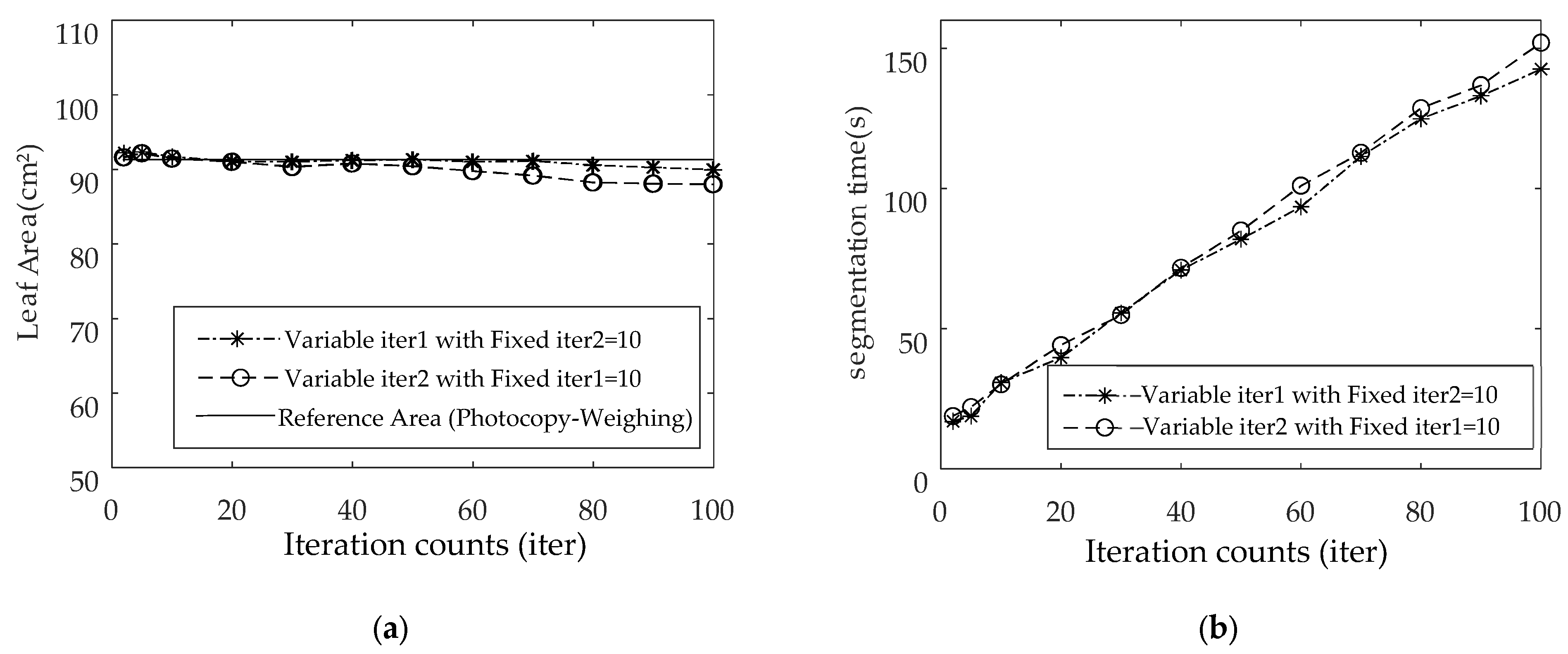
Two extended experiments were conducted: (a) iter₁ fixed at 10 with iter₂ varying from 2 to 100, and (b) iter₂ fixed at 10 with iter₁ varying similarly. Each configuration was executed 10 times to compute average leaf area and segmentation time. Results indicate that increasing either iter₁ or iter₂ independently leads to decreased estimated leaf area and linearly increased computation time (Figure 10). Optimal performance requires avoiding extreme values: insufficient iter₁ causes incomplete segmentation, while excessive iter₁ prolongs runtime without improving accuracy; insufficient iter₂ reduces contour smoothness, and too many iter₂ iterations waste computation without enhancing convergence. In practice, iter₁ should be set to allow the curve to approach the leaf margin, followed by a moderate iter₂ to ensure stable and smooth convergence.

4.5. Impact of Shooting Angle and Height

This study examines the effect of varying shooting angles and heights on tomato leaf area measurements using a fixed parameter set (p = 0.2, r = 50p, c₁ = 3, c₂ = 1, iter₁ = 4, iter₂ = 6). The same leaf was photographed from multiple angles and heights, both intact and after being cut. For each image, leaf area was computed 10 times to determine the average value, average segmentation time, and corresponding standard deviations.

As shown in

Table 13. Experimental results under different shooting angles and heights.

Orig. Image	Hough Lines	Rect. Image	Meas. Mean Area (cm2)	Meas. Mean Time(s)
			137.37	21.16
			137.61	20.94
			136.26	20.32
			136.10	19.89
			137.50	20.79

, the standard deviations for both average leaf area and segmentation time remained below 1 across all shooting conditions, demonstrating high measurement stability and consistency. These findings confirm that the method is robust to variations in both shooting angle and height and effectively measures leaf area for both intact and cut leaves.

4.6. Impact of Leaf Color Variation

This study investigates the impact of leaf color variation on segmentation performance using pear tree leaves with significant color differences as examples. All original images were of equal size, and experiments were conducted with fixed parameters: p = 0.2, r = 50p, c₁ = 3, c₂ = 1, Iter₁ = 1, Iter₂ = 5.

As shown in

Table 14. Experimental results for pear leave with different colors.

Orig. Image	Hough Lines	Rect. Image	Auto-Init. Cont.	Fin. Cont.	Leaf Fin. Seg.	Meas. Area (cm2)	Meas. Time (s)	GT 1 Area (cm2)	AE (cm2)
						54.75	9.98	54.72	0.03
						29.87	12.56	29.55	0.32
						37.19	10.30	37.33	0.14
						27.26	8.65	26.65	0.61
						42.22	8.80	43.03	0.81

¹ GT = Ground Truth, obtained via manual photocopy-weighing technique.

, leaves of different colors from the same crop species were successfully extracted with high accuracy. The measured leaf areas showed close agreement with GT areas, with all relative errors (AE) remaining below 1 cm². The segmentation time was found to be independent of original image size but correlated with the size of the corrected images after Hough transformation.

4.7. Performance Evaluation of Different Approaches

In contrast to threshold-based techniques that are sensitive to lighting and color variations, our model makes full use of color information to enhance robustness. Unlike deep learning approaches, our method requires no training, is species-agnostic, and maintains complete operational transparency. Compared to OpenPheno, which offers full automation but lacks parameter adjustability, and ImageJ, which depends heavily on manual intervention and yields operator-dependent results, our solution strikes an optimal balance by combining automation with flexible user control. By integrating automated geometric correction, intuitive interaction, and statistically driven segmentation, our system outputs both leaf and reference contours overlaid on the original image for real-time visual verification—a feature rarely supported in existing solutions.

5. Conclusions

This study presents a general leaf area measurement system and examines the influence of various parameters on measurement results. Experiments show that image rectification improves the accuracy of leaf area measurement and reduces errors. Manual sampling helps acquire prior knowledge about the leaves. The level set-based curve evolution method not only allows visual inspection of leaf extraction but also increases computational efficiency. The standard deviation of leaf area measurements remained below 1 cm² under different sampling points, initial contours, scaling factors, shooting angles, and heights, indicating high stability. The root mean square error (RMSE), using manual photocopy-weighing as the reference method, was associated with the complexity of the leaf margin—more complex edges led to larger RMSE values. Segmentation time was mainly affected by the size of the rectified image, the scaling factor, and the number of iterations. Specifically, processing time increased approximately exponentially with the scaling factor and linearly with the number of iterations. Too few iterations prevented the curve from reaching the leaf edge, while too many resulted in prolonged computation without noticeable improvement. Automating the selection of iteration counts requires further investigation and remains a limitation of the proposed method. Another drawback is the need to detach leaves for imaging; future research should explore non-destructive image acquisition techniques.

References

1. Jiang, N. A Non-Destructive Method for Toal Green Leaf Area Estimation of Individual Rice Plants. Ph.D. Dissertation, Huazhong University of Science and Technology, Wuhan, China, 2014. [Google Scholar]
2. Yin, C.; Shi, Z.; Tian, C.; Chen, C.; Li, D.; Dong, W.; Zhang, Y. Effects of Red and Blue Light on Photosynthetic Carbon Assimilation and Growth Development in Plants: A Review. Chin. J. Appl. Ecol. 2025, 36, 2246–2256. [Google Scholar] [CrossRef]
3. Shi, Y.; Xia, C. Research on Leaf Area Measurement of Variable Reference Based on Checkerboards. J. Chin. Agric. Mech. 2021, 42, 191–196. [Google Scholar] [CrossRef]
4. Zhang, F.; Li, X.; Zhao, Q.; Feng, Y.; Wu, Y. Regression Estimation on Leaf Area of Hevea Brasiliensis Clones. Trop. Agric. Sci. Technol. 2024, 47, 63–68. [Google Scholar] [CrossRef]
5. Zhang, Z.; Jia, S.; Zhao, N.; Liu, S.; Fan, F.; Nie, L. A Measurement Approach of Leaf Area Based on Digital Image Processing and Regression Equation of Leaves Area on Watermelon. China Cucurbits Veg. 2021, 34, 51–54. [Google Scholar] [CrossRef]
6. Li, Q.; Yang, M.; Yuan, P.; Xue, Y. Image Measurement Method of Leaf Area Based on Saturation Segmentation. J. For. Eng. 2021, 6, 147–152. [Google Scholar] [CrossRef]
7. Xu, Z.; Sun, L.; Li, B.; Lin, J.; Lan, W.; Zhang, S. Design of Leaf Area Measurement System Based on Android Smartphone. Exp. Technol. Manag. 2023, 40, 89–94. [Google Scholar] [CrossRef]
8. Tan, X.; Tan, L.; Yang, S. Leaf Area Measurement Method Based on Black-White Scanning Image. J. Guangxi Agric. 2022, 37, 46–52. [Google Scholar]
9. Li, F.; Li, J.; Huang, H.; Guan, M.; Guan, C. Research on Non-Destructive Measurement Methods and Strategies of Individual Rape Leaf Area in Field. Acta Laser Biol. Sin. 2021, 30, 505–517. [Google Scholar]
10. Wang, P.; Deng, H.; Guo, J.; Ji, S.; Meng, D.; Bao, J.; Zuo, P. Leaf Segmentation Using Modified YOLOv8-Seg Models. Life 2024, 14, 780. [Google Scholar] [CrossRef]
11. Huang, F.; Li, Y.; Liu, Z.; Gong, L.; Liu, C. A Method for Calculating the Leaf Area of Pak Choi Based on an Improved Mask R-CNN. Agriculture 2024, 14, 101. [Google Scholar] [CrossRef]
12. Khan, A.T.; Jensen, S.M. LEAF-Net: A Unified Framework for Leaf Extraction and Analysis in Multi-Crop Phenotyping Using YOLOv11. Agriculture 2025, 15, 196. [Google Scholar] [CrossRef]
13. Guo, X.; Cheng, J.; Wang, L. Research and Realisation the Statistics Algorithm of Wheat Leaf Area. J. Henan Inst. Sci. Technol. Sci. Ed. 2019, 47, 56–59. [Google Scholar]
14. Yang, Z.; Yang, P.; Zhang, M.; Xiao, Y.; Liu, H. Study on Correction Method of Local Geometric Distortion in Projection Phantom Imaging. Acta Photonica Sin. 2022, 51, 0311004. [Google Scholar]
15. Zhou, D.; Yang, Y.; Zhu, J.; Wang, K. Tilt Correction Method of Pointer Meter Based on Deep Learning. J. Comput.-Aided Des. Comput. Graph. 2020, 32, 1976–1984. [Google Scholar] [CrossRef]
16. Matarneh, S.; Elghaish, F.; Al-Ghraibah, A.; Abdellatef, E.; Edwards, D.J. An Automatic Image Processing Based on Hough Transform Algorithm for Pavement Crack Detection and Classification. Smart Sustain. Built Environ. 2025, 14, 1–22. [Google Scholar] [CrossRef]
17. Sasmita, W.A.; Mubarok, H.; Widiyasono, N. Agricultural Path Detection Systems Using Canny-Edge Detection and Hough Transform. IAES Int. J. Robot. Autom. 2024, 13, 247. [Google Scholar] [CrossRef]
18. Wang, P.; Liu, Z.; Ma, C.; Peng, A.; Ren, F.; Cai, M. Investigation of Fast Identification of Joint Traces Information of Rock Mass Based on Hough Detection Method and Its Application. Rock Soil Mech. 2022, 43, 2887–2897. [Google Scholar] [CrossRef]
19. Cremers, D.; Rousson, M.; Deriche, R. A Review of Statistical Approaches to Level Set Segmentation: Integrating Color, Texture, Motion and Shape. Int. J. Comput. Vis. 2007, 72, 195–215. [Google Scholar] [CrossRef]
20. Qu, H.-B.; Xiang, L.; Wang, J.-Q.; Li, B.; Tao, H.-J. Variational Bayesian Level Set for Image Segmentation. In Proceedings of the International Conference on Machine Vision, London, UK, 24 December 2013; p. 90670D. [Google Scholar]
21. Chan, T.F.; Vese, L.A. Active Contours without Edges. IEEE Trans. Image Process. 2001, 10, 266–277. [Google Scholar] [CrossRef] [PubMed]
22. Ben Ayed, I.; Hennane, N.; Mitiche, A. Unsupervised Variational Image Segmentation/Classification Using a Weibull Observation Model. IEEE Trans. Image Process. 2006, 15, 3431–3439. [Google Scholar] [CrossRef]
23. Reska, D.; Kretowski, M. GPU-Accelerated Image Segmentation Based on Level Sets and Multiple Texture Features. Multimed. Tools Appl. 2021, 80, 5087–5109. [Google Scholar] [CrossRef]
24. Han, T.; Cao, H.; Yang, Y. AS2LS: Adaptive Anatomical Structure-Based Two-Layer Level Set Framework for Medical Image Segmentation. IEEE Trans. Image Process. 2024, 33, 6393–6408. [Google Scholar] [CrossRef] [PubMed]
25. Joshi, A.; Saquib Khan, M.; Choi, K.N. Medical Image Segmentation Using Combined Level Set and Saliency Analysis. IEEE Access 2024, 12, 102016–102026. [Google Scholar] [CrossRef]
26. Li, W.; Liu, W.; Zhu, J.; Cui, M.; Hua, X.-S.; Zhang, L. Box2Mask: Box-Supervised Instance Segmentation with Level Set Evolution, Proceedings of the Computer Vision—ECCV 2022. Tel Aviv, Israel, 23–27 October 2022; Springer Nature: Cham, Switzerland, 2022; pp. 1–18. [Google Scholar]
27. Aghazadeh, N.; Moradi, P.; Castellano, G.; Noras, P. An Automatic MRI Brain Image Segmentation Technique Using Edge–Region-Based Level Set. J. Supercomput. 2023, 79, 7337–7359. [Google Scholar] [CrossRef]
28. Olfa, B.; Ziad, B.; Nozha, B. Adaptive Satellite Images Segmentation by Level Set Multiregion Competition. Inst. Natl. Rech. Inform. Autom. 1992, 37, 55–57. [Google Scholar] [CrossRef]
29. Li, C.; Xu, C.; Gui, C.; Fox, M.D. Distance Regularized Level Set Evolution and Its Application to Image Segmentation. IEEE Trans. Image Process. 2010, 19, 3243–3254. [Google Scholar] [CrossRef]
30. He, A.; Li, B.; Xu, Z.; Yang, Y.; Li, Z. Detection of Bamboo Leaf Area Based on Self-Made Colored Base Plate and Spectral Features. Res. Explor. Lab. 2024, 43, 39–44. [Google Scholar] [CrossRef]
31. Hu, T.; Shen, P.; Zhang, Y.; Zhang, J.; Li, X.; Xia, C.; Liu, P.; Lu, H.; Wu, T.; Han, Z. OpenPheno: An Open-Access, User-Friendly, and Smartphone-Based Software Platform for Instant Plant Phenotyping. Plant Methods 2025, 21, 76. [Google Scholar] [CrossRef]
Figure 1. Leaves of the same plant species exhibiting varying shades of green (specifically pear tree leaves).
Agriculture 15 02101 g001
Figure 2. Leaves of different crops exhibiting diverse morphologies: (a) Tomato leaf; (b) Broomcorn millet leaf; (c) Grape leaf; (d) Pear tree leaf.
Agriculture 15 02101 g002
Figure 3. Flowchart of leaf area calculation.
Agriculture 15 02101 g003
Figure 4. The leaf-bearing platform with a reference marker.
Agriculture 15 02101 g004
Figure 5. Image rectification process: (a) Original image; (b) Binary image; (c) Edge image; (d) Hough line detection; (e) Rectified image.
Agriculture 15 02101 g005
Figure 6. Representation of a partition, the curves in different colors represent the zero-level contours of two distinct level set functions.
Agriculture 15 02101 g006
Figure 7. Interactive Visual Application Interface: (a) EXE Application Interface; (b) Web Application Interface.
Agriculture 15 02101 g007aAgriculture 15 02101 g007b
Figure 8. Rough segmentation regions of a broomcorn millet: (a) Original Image; (b) Hough-Detected lines; (c) Manual seed points; (d) Leaf rough segmentation; (e) Reference rough segmentation.
Agriculture 15 02101 g008
Figure 9. Segmentation time and Leaf area with scaling factor (p): (a) Segmentation time with p; (b) Leaf area with p.
Agriculture 15 02101 g009
Figure 10. Leaf area measurements and Segmentation time under different iteration counts (iter): (a) Leaf area measurements with iter; (b) Segmentation time with iter.
Agriculture 15 02101 g010