Changes in Camelina sativa Yield Based on Temperature and Precipitation Using FDA

Abstract

Camelina (Camelina sativa) is an oilseed crop of increasing importance, valued not only for its adaptability to diverse environmental conditions and potential for sustainable agriculture but also for its economic advantages, including low input requirements and suitability for biofuel production and niche markets. This study examines the relationship between camelina yield and climatic variables—specifically temperature and precipitation—based on a ten-year field experiment conducted in Poland. To capture the temporal dynamics of weather conditions, Functional Data Analysis (FDA) was applied to daily temperature and precipitation data. The analysis revealed that yield variability was strongly influenced by the length of the vegetative period and specific weather patterns in April and July. Higher yields were recorded in years characterized by moderate spring temperatures, elevated temperatures in July, and evenly distributed rainfall during the early generative growth stages. The Maximal Information Coefficient ($\mathrm{M}\mathrm{I}\mathrm{C}$) confirmed the relevance of these variables, with the duration of the vegetative phase showing the strongest correlation with yield. Cluster analysis further distinguished high- and low-yield years based on functional weather profiles. The FDA-based approach provided clear, interpretable insights into climate–yield interactions and demonstrated greater effectiveness than traditional regression models in capturing complex, time-dependent relationships. These findings enhance our understanding of camelina’s response to climatic variability and support the development of predictive tools for resilient, climate-smart crop management.

1. Introduction

According to the latest data from the European Commission and Eurostat, in 2025 the crop structure in the European Union is dominated by cereals, particularly common wheat, barley, and maize, which together account for approximately 54% of the total sown area. Oilseed crops rank second, covering around 13% of the area (primarily winter rapeseed, sunflower, and soybean), followed by legumes and fodder crops (about 6%) and root crops (approximately 4%).

Although the Biodiversity Strategy for 2030 and the European Green Deal aim to promote crop diversity, statistics from Eurostat, FAO, and the World Bank indicate a serious decline in crop biodiversity across Europe over the last decades. This trend reflects the long-term intensification and specialization of agricultural production, which has led to the dominance of a limited number of crop species and the marginalization of traditional and regionally adapted varieties [1]. Despite certain challenges in coordinating or integrating biodiversity goals with other sectoral policies, a gradual expansion in the cultivation of less common crop species is now observable, particularly in organic farming systems and research-driven pilot programs.

Camelina (Camelina sativa) is an annual oilseed crop native to Eastern Europe and Asia. Historically, it was the second most cultivated oilseed in Poland until the 1950s, primarily used for food purposes. Its cultivation declined with the rise of higher-yielding crops. However, due to its exceptional adaptability to diverse soil and climatic conditions, as well as its expanding range of industrial and environmental applications, camelina has recently regained attention in European agriculture [2].

In addition to its traditional uses, camelina is now recognized as a promising non-food oilseed crop for the production of bioproducts and biofuels, including biodiesel and sustainable aviation fuel. Its oil, meal, and straw are also utilized in animal feed, functional foods, dietary supplements, biogas, ethanol, energy pellets, compost, bio-lubricants, cosmetics, and industrial chemicals [3]. Oil extraction is typically performed via cold or hot pressing, or solvent-based methods (e.g., hexane, supercritical CO₂). Seed oil content varies between 32% and 50% in spring varieties and 36% and 43% in winter varieties, depending on genotype and environmental conditions [4,5,6,7,8]. The resulting press cake contains approximately 10% fat, 45% protein, 13% fiber, 5% minerals, and notable levels of glucosinolates (13.2–36.2 μmol/g) and phytates (1–6%) [9,10,11].

Although both spring and winter forms of camelina exist, commercial cultivation is dominated by spring types, which are characterized by a short growing season and strong resistance to biotic and abiotic stressors [12,13,14,15]. Camelina is considered one of the most disease- and pest-resistant oilseed crops [16].

Due to its adaptability to low-fertility soils, camelina is a viable alternative to rapeseed on marginal lands. Seed yields range from 1.3 to 3.3 Mg dry matter per hectare, depending on genotype and site conditions [2,17,18,19]. Oil yields range from 540 to 1410 kg/ha, exceeding those of soybean and approaching those of rapeseed [20].

This study investigates how camelina yield responds to time-dependent environmental factors, mainly temperature and precipitation. Understanding these relationships is crucial for assessing the effects of climate change on crop production. Different modeling approaches often produce inconsistent results, which highlights the need for precise analysis of climate–yield interactions. Most studies use seasonal averages of temperature and precipitation. Here, we instead analyze daily weather data recorded throughout the growing period of C. sativa. By treating these variables as time-dependent functions, we capture more detailed environmental dynamics. For this purpose, we apply Functional Data Analysis (FDA), following the method proposed by [21]. In recent years, scientists have been increasingly turning to modern statistical tools that use analyses based on the conversion of discrete data into continuous data. FDA enables the representation of continuous observations—here, temperature and precipitation—over time, preserving the richness of the data’s internal structure. This leads to a more precise and realistic interpretation of dynamic phenomena. In this paper, we use FDA to assess how changes in these environmental variables over the growing season have affected camelina yield across the studied years.

Today, FDA is widely used in the analysis of time-series data across multiple disciplines, including the life sciences [22,23]. Traditionally, the influence of climate variability on crop yields at the field level has been assessed using regression-based models. While effective, these models rely on strong assumptions and can result in substantial forecasting errors. In this study, we explore an innovative application of FDA to link field-level camelina yields with daily-scale weather data. To our knowledge, this approach has not been previously applied in studies on camelina yield, and it offers a novel method for capturing the complex dynamics between climate and crop performance.

In the literature, some papers with methods based on functional data are available. Authors are increasingly turning to such methods. An example that can be cited here is the work [24] based on strawberry and tomato production on the basis of year-round cultivation. The authors applied FDA to create a model that evaluates the impact of environmental parameters on crop yield in longitudinal cultivation. The model addresses the challenge of environmental fluctuations and provides interpretable results. This information can be used to optimize growth conditions, improve resource efficiency, and support sustainable development. Moreover, in [25], the authors applied a flexible machine learning approach. They combined Functional Principal Component Analysis with Random Forest to link field-scale wheat yield to local daily climate variables. FDA is widely used to analyze, model, and forecast data presented as time series. Its usefulness is confirmed by numerous scientific studies that employ this method. Among several review papers that also discuss its application, it is worth noting the work of [26], which highlights key aspects of FDA. The authors reviewed 11 electronic databases and identified studies on FDA applications published in peer-reviewed journals between 1995 and 2010.

2. Materials and Methods

2.1. Plant Material

The Polish Camelina sativa cultivar ‘Omega’ was used as the plant material in this study. It was developed at the Department of Genetics and Plant Breeding of the Poznań University of Life Sciences (PULS) and registered in Poland in 2013.

2.2. Field Experiment

The field experiment was conducted at the Agricultural Research Station in Dłoń (Poznań University of Life Sciences, Poland; 51°41′37″ N, 17°04′06″ E) over the 2015–2024 growing seasons. The climate of Greater Poland is classified as transitional between oceanic and continental types, resulting in considerable variability in weather conditions, including irregular precipitation and large air temperature amplitudes. This region exhibits a trend of increasing average air temperatures. The average annual air temperature in Greater Poland is approximately 8.8 °C, and the annual precipitation total does not exceed 600 mm, which categorizes this area as one of the driest regions in Poland. The experimental plots were located on soils classified as Haplic Luvisols (LVh) according to the World Reference Base for Soil Resources [27]. The preceding crop was soybean.

Camelina was sown at a depth of 15 mm using a small plot drill, with a seeding rate of 5 kg/ha. The seed used had a germination rate of ≥90%. Sowing was carried out annually between 26 March and 11 April. Prior to sowing, 50 kg/ha of P₂O₅ and 40 kg/ha of K₂O were applied. Nitrogen was supplied in three doses: 30 kg/ha before sowing, 40 kg/ha at the tillering stage, and 40 kg/ha prior to flowering.

Following sowing, the herbicide Butisan Star Max 500 SE—containing Quinmerac (100 g/L), Dimethenamid-P (200 g/L), and Metazachlor (200 g/L)—was applied. All agronomic procedures, including sowing density, tillage, and harvesting, were conducted according to a consistent protocol across all seasons. No pest or disease infestations were observed during the experiments, and no plant protection treatments were necessary.

Plants remained in the field until full ripening and were harvested using a Hege 125 combine harvester once they reached full maturity, defined as the stage when more than 90% of the silicles had dried and turned brown, and the majority of seeds exhibited a reddish-brown coloration.

The dates of flowering and maturity were recorded using the BBCH scale. Yield data were collected from plots ranging from 0.5 to 2.0 hectares, which were used for seed multiplication of the ‘Omega’ cultivar.

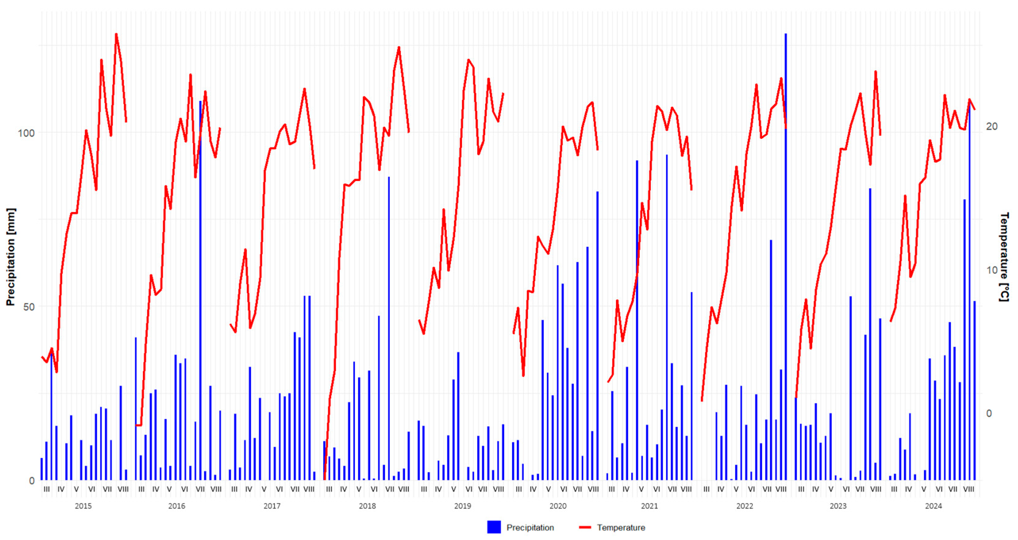
Average daily temperature and precipitation data (2005–2020) were recorded in accordance with WMO guidelines using a Vantage Vue 6357 UE 9 meteorological station (Davis Instruments, USA), located approximately 400 m from the experimental field. Atmospheric conditions, vegetation period lengths, and yield data from 2015 to 2024 are presented in Figure 1.

2.3. Statistical Analysis

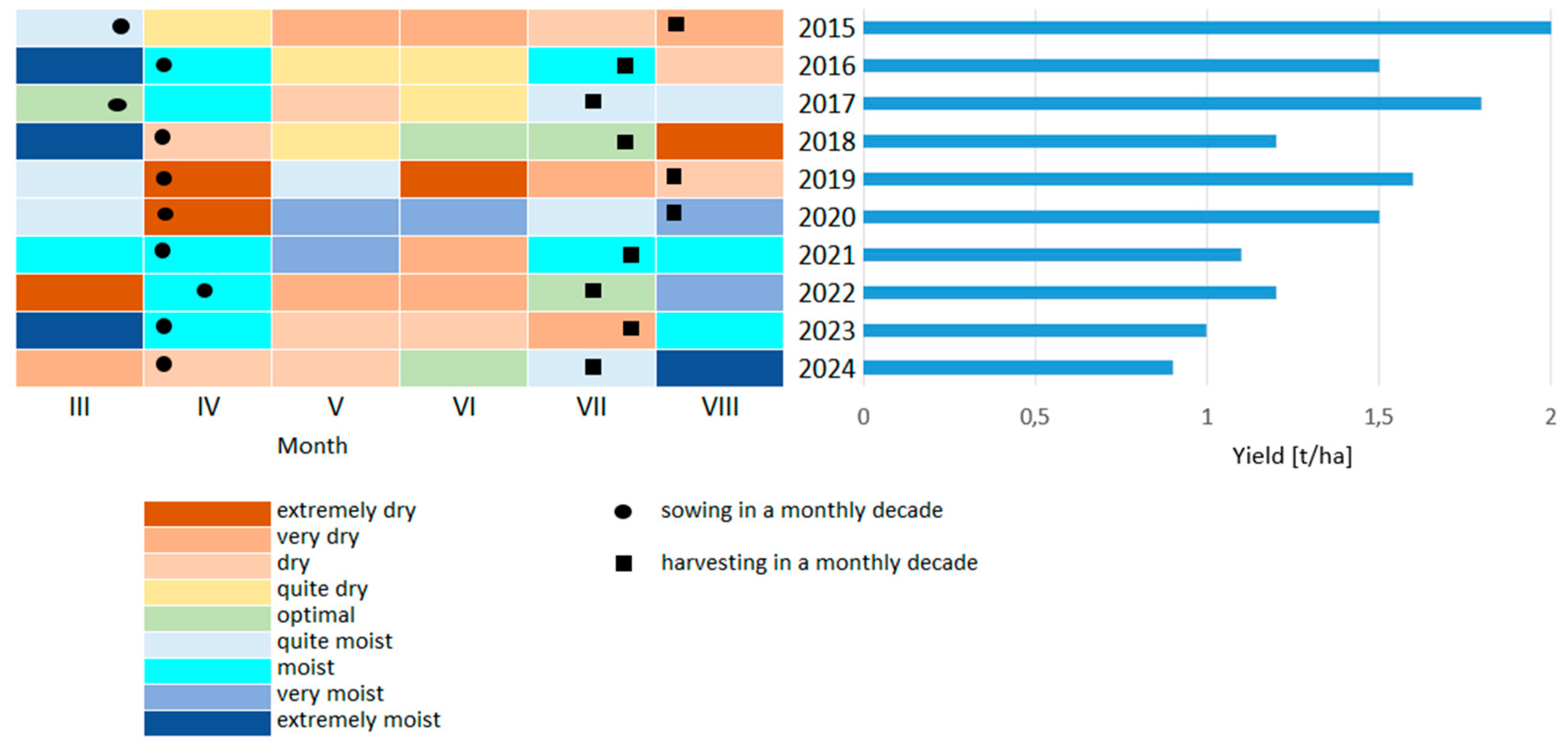
The collected data on air temperature and precipitation were used to determine the hydrothermal coefficient of Selyaninov [27,28] according to the formula $\mathrm{H}\mathrm{T}\mathrm{C}=R·10/\sum t$, where $R$ is the monthly precipitation in millimeters and $\sum t$ is the sum of daily average air temperatures in a given month in degrees Celsius. The coefficient is a measure of the effectiveness of precipitation in subsequent months of the growing season and allows for the separation of different types of plant growth and development conditions, in particular extreme and optimal conditions [29]. In order to interpret the $\mathrm{H}\mathrm{T}\mathrm{C}$ coefficient results, the following criterion was used: extremely dry $\mathrm{H}\mathrm{T}\mathrm{C}$ < 0.4, very dry $\mathrm{H}\mathrm{T}\mathrm{C}\in \left(0.4,0.7⟩\right.$, dry $\mathrm{H}\mathrm{T}\mathrm{C}\in \left(0.7,1.0⟩\right.$, quite dry $\mathrm{H}\mathrm{T}\mathrm{C}\in \left(1.0,1.3⟩\right.$, optimal $\mathrm{H}\mathrm{T}\mathrm{C}\in \left(1.3,1.6⟩\right.$, quite humid $\mathrm{H}\mathrm{T}\mathrm{C}\in \left(1.6,2.0⟩\right.$, humid $\mathrm{H}\mathrm{T}\mathrm{C}\in \left(2.0,2.5⟩\right.$, very humid $\mathrm{H}\mathrm{T}\mathrm{C}\in \left(2.5,3.0⟩\right.$, extremely humid $\mathrm{H}\mathrm{T}\mathrm{C}\ge 3.0$.

A dendrogram was employed to identify the years that exhibit the greatest similarity with respect to the studied variables, namely temperature and precipitation. It is a tree representation of data that groups objects based on their similarity, obtained by applying hierarchical clustering methods. Grouping is carried out gradually, from determining the most similar objects to combining all objects into one group. In a dendrogram, clusters at one level are combined with each other to create clusters at the next levels [30].

Functional Data Analysis (FDA) allows each unit of data to be analyzed as a continuous curve represented by a function transformed from a series of continuously recorded data [31]. Here, daily temperatures and precipitation are observed over the growing season for many years. Thus, the curves representing the time course of temperature and precipitation in each year are considered a data series. The most important idea of the FDA is to transform the data recorded as repeated measurements over time into functions for each year, and in the next step we analyze the set of functions. Let $y_{ijk}$ denotes the observed value of $k^{th}$ variable $k\in \left\{Temperature, Precipitation\right\}$ measured on $i^{th}$ statistical unit, $i=2015, 2016, \dots ,2024$, in $j^{th}$ time point, $j\in \left\{1\mathrm{I}\mathrm{I}\mathrm{I}, 2\mathrm{I}\mathrm{I}\mathrm{I},\dots ,31\mathrm{V}\mathrm{I}\mathrm{I}\mathrm{I}\right\}.$ In such a case, our data is pair $\left\{t_{ijk}, y_{ijk}\right\}, t_{ijk}\in 〈0, T〉$. However, in many cases it is more convenient to use continuous time functions $x\left(t\right), t\in 〈0, T〉.$ In such a case, we are dealing with functional data [32]. Typically, functional data consist of N independent realizations $\left\{x_{ik}\left(t\right), t\in 〈0, T〉, i=2015, 2016, \dots ,2024\right\}$ of some random process $X\left(t\right)$. In such a situation, we can convert discrete data $\left\{t_{ijk}, y_{ijk}\right\}$ to functional data $x_{ik}\left(t\right).$ Conversion from discrete data to continuous functions requires smoothing [33]. The smoothing parameter was selected using Generalized Cross-Validation (GCV) in such a way as to balance fit and smoothness. At the same time, efforts were made to prevent overfitting while preserving significant patterns in the data. For validation, RMSE was also computed across a grid of λ values, and the results confirmed consistency between both approaches. We perform the conversion process for each $i$ and $k$ separately. In the first step, we create a database of B-splines functions, which will be used to represent functional data. It is worth mentioning that for data with irregular patterns in time series related to the environment, B-spline basis functions are most commonly used. They were chosen for their flexibility and computational efficiency. This basis will later be used to approximate the functional data using a linear combination of basis functions. Then, the mean function is calculated for a set of functional data. As a result, figures show smooth curves that represent the average course of the data over time.

The Maximal Information Coefficient ($\mathrm{M}\mathrm{I}\mathrm{C}$) is a tool for finding the strongest pairwise relationships in a dataset with many variables [34,35,36,37]. The definition of MIC is based on a naive mutual information estimate ${\mathrm{I}}_{\mathrm{M}\mathrm{I}\mathrm{C}}\left\{x,y\right\}$ computed using a data-dependent binning scheme. Let $n_x$ and $n_y$, respectively, denote the number of bins imposed on the $x$ and $y$ axes. The MIC binning scheme is chosen so that the total number of bins $n_x{n}_y$ does not exceed some user-specified value B and the value of the ratio $\mathrm{M}\mathrm{I}\mathrm{C}\left\{x,y\right\}={\displaystyle \frac{{\mathrm{I}}_{\mathrm{M}\mathrm{I}\mathrm{C}}\left\{x,y\right\}}{{\mathrm{Z}}_{\mathrm{M}\mathrm{I}\mathrm{C}}}},$ where ${\mathrm{Z}}_{\mathrm{M}\mathrm{I}\mathrm{C}}={log}_2\left(min\left(n_x,n_y\right)\right)$ is maximized. $\mathrm{M}\mathrm{I}\mathrm{C}$ is useful because it gives similar scores to equally noisy relationships of different types. This property, called equitability, is important for analyzing high-dimensional datasets. $\mathrm{M}\mathrm{I}\mathrm{C}$ takes values between 0 and 1, where 0 means statistical independence and 1 means a completely noiseless relationship. $\mathrm{M}\mathrm{I}\mathrm{C}$ belongs to a larger class of Maximal Information-based Nonparametric Exploration (MINE) statistics for identifying and classifying relationships. The $\mathrm{M}\mathrm{I}\mathrm{C}$ is interpreted as the percent of a variable Y that can be explained by a variable X. $\mathrm{M}\mathrm{I}\mathrm{C}$ assigns the same score to equally noisy relationships, regardless of the type of relationship. This is important in cases when the distribution of data or the nature of relationships between variable is not determined [38,39]. We determine $\mathrm{M}\mathrm{I}\mathrm{C}$ according to the formula given in [40] and determine in the minerva package in R [41]. We compare the value of $\mathrm{M}\mathrm{I}\mathrm{C}$ with the Mutual Information (MI) coefficient [42], and we use the infotheo package in R Version R 4.5.0 to compare the results [43].

3. Results

3.1. Weather Variability and Phenological Development

During the study period, substantial interannual weather variability was observed, including extreme precipitation events and temperature fluctuations (see Figure 2). These conditions significantly influenced the phenological development and seed yield of the camelina (Camelina sativa) cultivar Omega. Although agronomic practices were standardized across all seasons, other factors, such as slight variability in sowing dates (ranging from 26 March to 11 April), the occurrence of extreme weather events (e.g., heavy rainfall or drought), and potential soil fertility carryover effects, may have contributed to yield differences.

Harvest maturity was recorded between 18 July and 8 August, with the crop cycle lasting from 99 days in 2022 to 129 days in 2015. Seed yields ranged from 0.9 t/ha (2024) to 2.0 t/ha (2015). Total precipitation during the growing season varied widely, falling below 200 mm in 2015 and 2019, and exceeding 370 mm in 2016, 2020, and 2021. Both extremely dry (e.g., 167.2 mm in 2019) and extremely wet seasons were recorded. Notable extreme events included 37.5 mm of rainfall in late March 2015, shortly after sowing, and complete absence of precipitation in March 2022, which likely affected seedling establishment.

3.2. Hydrothermal Conditions and Selyaninov Coefficient

The relationship between precipitation and temperature was assessed using the Selyaninov Hydrothermal Coefficient ($\mathrm{H}\mathrm{T}\mathrm{C}$), as shown in Figure 3$\mathrm{H}\mathrm{T}\mathrm{C}$ values revealed considerable variability throughout the camelina growing season, particularly during sowing and harvest periods. March was classified as extremely humid in 2016, 2018, and 2023, while April was wet in 2016, 2017, 2021, 2022, and 2023. In contrast, May and June were often quite dry or very dry.

April conditions are critical for germination and early vegetative growth. Excess moisture may delay emergence or promote fungal pressure, while drought can reduce stand density. July, corresponding to the seed-filling phase, is particularly sensitive to heat and water stress. Optimal conditions in July were observed only in 2018 and 2022, which coincided with higher yields, suggesting that favorable hydrothermal conditions during this period support efficient assimilate translocation and seed development.

Despite the use of a single camelina cultivar and uniform soil conditions, no clear long-term trends in $\mathrm{H}\mathrm{T}\mathrm{C}$ values were observed over the ten-year period. To better understand the influence of weather patterns, hierarchical clustering was applied to group the years based on temperature and precipitation profiles (Figure 4).

3.3. Cluster-Based Functional Analysis of Weather Patterns and Yield

Therefore, all years were divided based on hierarchical trees; see Figure 4. Here, Figure 4a illustrates the division of the studied years into two clusters based on the observed temperature values. For such a division, the average silhouette width is 0.7302. This means that the observation groups are coherent and well separated [44]. The first cluster comprises the years 2018, 2019, and 2024, while the second cluster includes the years 2015–2017, 2020, 2021, and 2023. Figure 4b shows the division of the years studied based on the observed precipitation values, and for this figure the average silhouette width equals 0.5654. Here, two clusters can be distinguished, the first covering the years 2015, 2019, 2022, and 2023, and the second covering the years 2016–2018, 2020, 2021, and 2024. In terms of temperature, four of the five years with higher yields, i.e., 2015–2017 and 2020, are in one cluster. In terms of precipitation, three of the five years with higher yields, i.e., 2016, 2017, and 2021, are in one cluster. The division into clusters resulting from hierarchical analysis is similar for both analyzed environmental features: temperature and precipitation.

The impact of the observed temperature and precipitation values shows significant heterogeneity in the analyzed period, characterized by significant differences depending on the specific year. The observed high variability made it impossible to adopt a uniform analytical model for the entire dataset. Therefore, in order to ensure greater accuracy and precision of interpretation, it was decided to divide the research data into two separate groups, corresponding to clearly different patterns of behavior over time. The results were divided into years depending on the yield obtained. The first group includes years in which the yield was above the overall average—1.5 t/ha or more—and the second group includes years in which the yield was below the average (the seed yield did not exceed 1.2 t/ha).

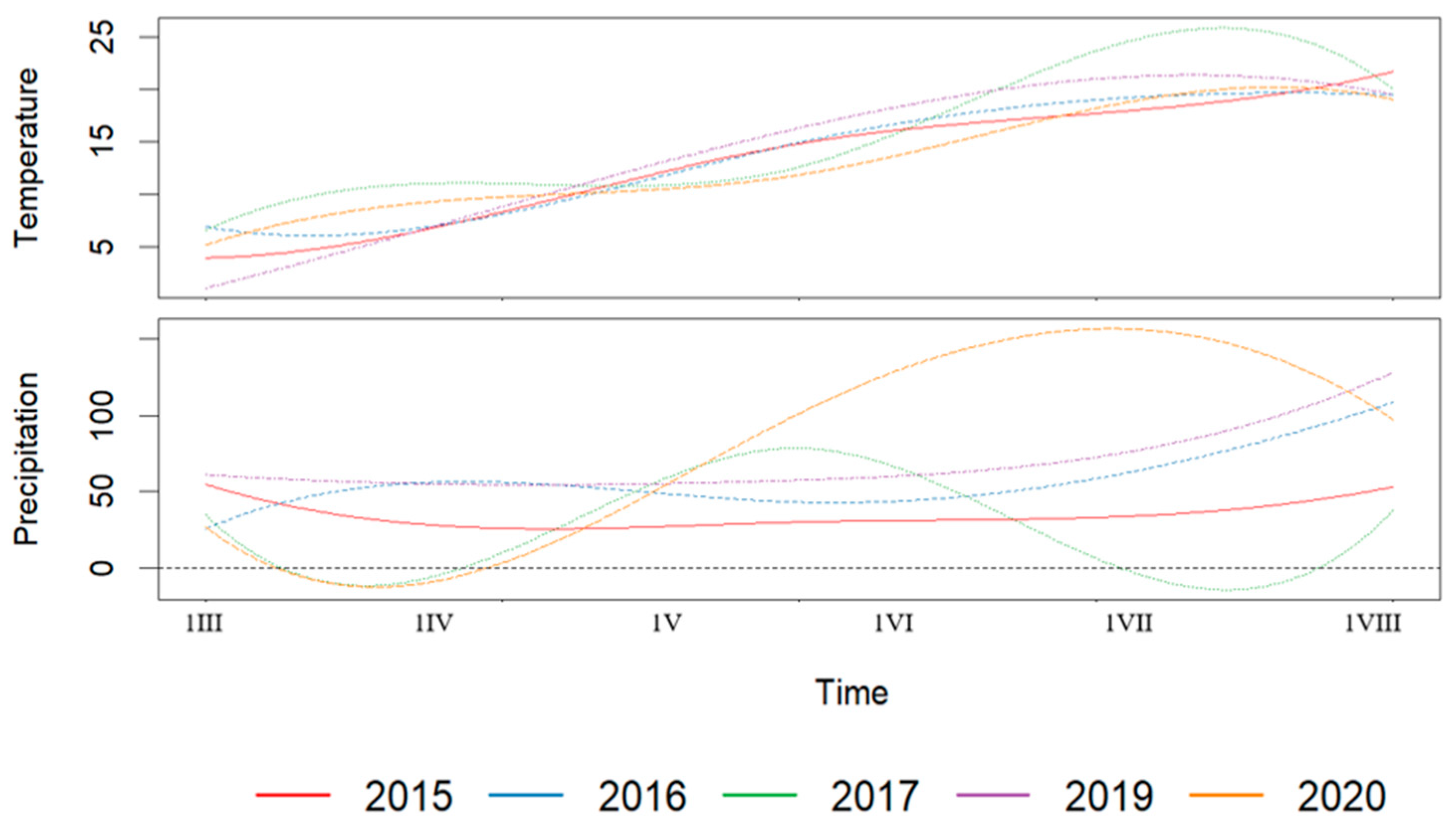
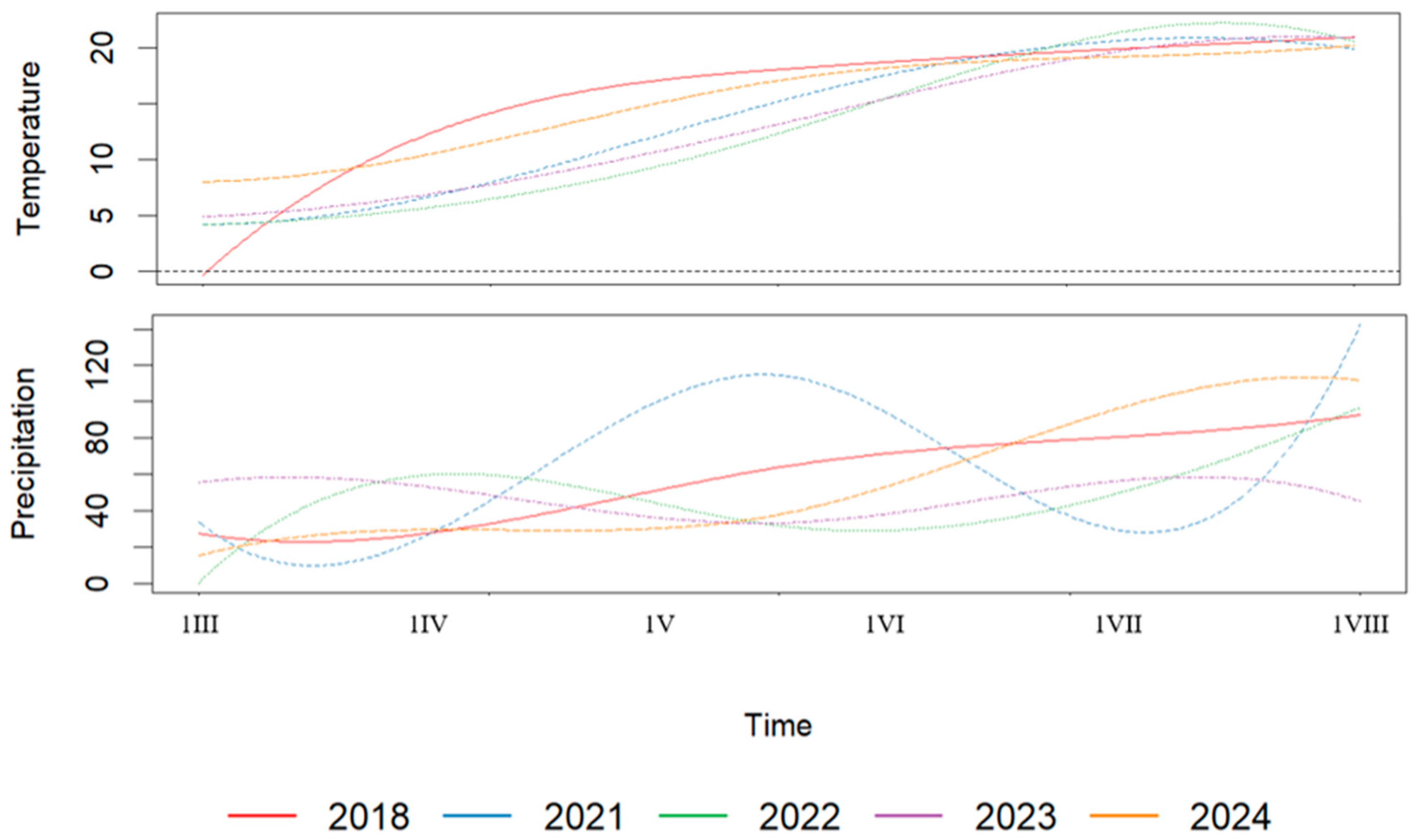
For each observed variable, i.e., temperature and precipitation, our data presented as a pair are converted to functional data [32]. This transformation was performed separately for each observed variable and for each year. The functions have been smoothed in accordance with [33], see

Table 1. The values of the smoothing parameter λ and RMSE determined for temperature (T) and precipitation (P) for high yield years (HYY) and low yield years (LYY).

	HYY	LYY
${\lambda }_T$ ${\mathrm{R}\mathrm{M}\mathrm{S}\mathrm{E}}_{\mathrm{T}}$	2.212 1.635	9.703 1.366
${\lambda }_P$ ${\mathrm{R}\mathrm{M}\mathrm{S}\mathrm{E}}_{\mathrm{P}}$	11.964 5.809	4.923 6.586

. To examine the relationship between weather conditions and seed yield, data were divided into high-yielding years (2015–2017, 2019, and 2020; mean yield = 1.68 t/ha) and low-yielding years (2018, 2021–2024; mean yield = 1.08 t/ha), based on the yield and clustering results presented in Figure 4.

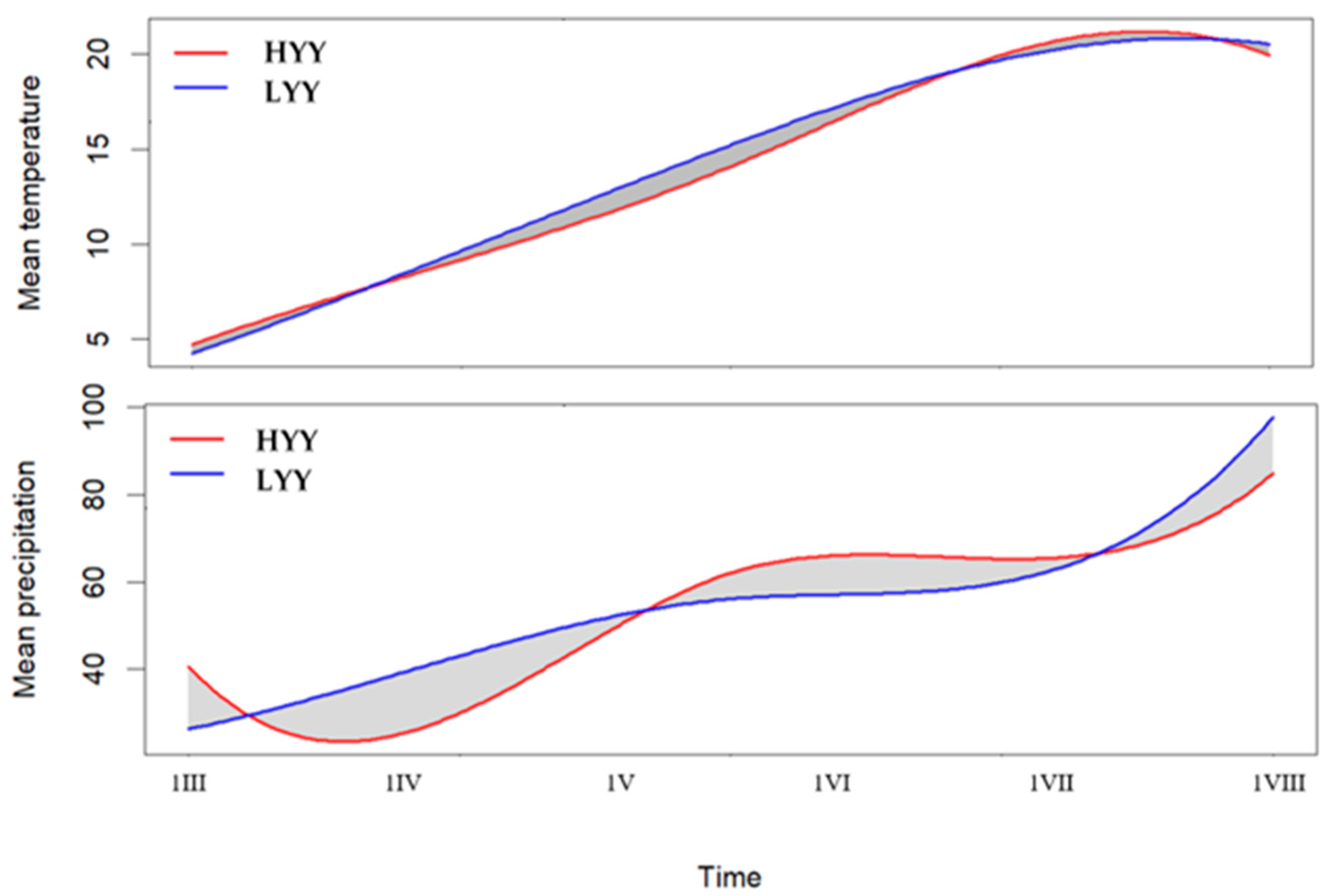
In Figures S1 and S2, the temperature functions for years 2015–2024 and the precipitation functions for years 2015–2024 are presented. Then, all years were divided based on hierarchical trees. Therefore, in Figure 5 and Figure 6, the functional data for temperature and precipitation for high- and low-yielding years, respectively, are presented. Moreover, in Figure 7 the comparisons of mean curves for temperature and precipitation determined for both yield groups are given. The resulting figures allow us to use the same graphs to identify the relationships between weather conditions in years that yielded higher or lower yields than the average. Using graphs of mean functions (Figure 7) allows us to draw more general conclusions indicating trends for the groups of years under consideration.

3.4. Environmental Stress Factors and Functional Modelling of Yield Response

Analysis of the presented graphs reveals greater variability in temperature and precipitation during years less favorable for camelina cultivation. In the graph comparing mean temperatures across years, it is evident that spring camelina yielded better when higher temperatures occurred in early March and June, while the remaining months were cooler compared to years with lower yields.

High yields were supported by rainfall preceding the sowing of the very small seeds, as well as precipitation in May and early June—during the period from the emergence of the first lateral shoots to full flowering.

In

Table 2. $\mathrm{M}\mathrm{I}\mathrm{C}$ determined for months and temperature and precipitation. NVD denotes number of vegetation days.

Yield	NDV	0.6099865
Yield	Month	Temperature	Precipitation
	March	0.2364528	0.2364528
	April	0.3958156	0.3958156
	May	0.2364528	0.2364528
	June	0.2364528	0.2364528
	July	0.3958156	0.1080315

, the Maximal Information Coefficient ($\mathrm{M}\mathrm{I}\mathrm{C}$) was calculated for individual months. $\mathrm{M}\mathrm{I}\mathrm{C}$ measures the strength of association between variables and ranges from 0 to 1, where 0 indicates statistical independence and 1 indicates a perfectly noiseless relationship. The strongest association was found between yield and the number of vegetative days, with a $\mathrm{M}\mathrm{I}\mathrm{C}$ value of 0.6099, indicating that the length of the vegetative period had the greatest impact on yield. The values of the $\mathrm{M}\mathrm{I}\mathrm{C}$ coefficient in the range of 0.3–0.6 indicate an average relationship between the variables. To verify its robustness, a comparison was made with the Mutual Information (MI) coefficient described in [41] in the infotheo package in R, and the values differed only slightly.

Comparing $\mathrm{M}\mathrm{I}\mathrm{C}$ values describing the relationship between vegetative duration, temperature, precipitation, and yield, the highest values highlight the critical role of April and July in shaping camelina seed yield (Table 2). The importance of temperature distribution in April and July, as well as precipitation in July, is further confirmed by Figure 5, Figure 6 and Figure 7. Lower temperatures in April combined with higher temperatures in July, along with increasing rainfall in April and reduced precipitation toward the end of the growing season, positively influenced the seed yield of spring camelina.

Here, a significant impact of the conditions prevailing in a given year on the manifestation of all evaluated traits was demonstrated. The authors mentioned that plant height is positively affected by precipitation during the germination–flowering period and in the 1st decade of June. Our experiment also observed a significant effect of weather conditions, but our conclusions were drawn using more advanced statistical tools. One of these was functional analysis, which is increasingly being used by scientists.

4. Discussion

It is well established that a plant’s response to drought or water stress is influenced by species, genotype, and the intensity and duration of the stress [45]. Within the Brassicaceae family, the effects of abiotic stress—particularly drought—on rapeseed yield have been extensively studied. For instance, Shekari et al. (2016) in [45] applied water deficit treatments during three successive growth stages: stem elongation, onset of flowering, and silique formation. The most pronounced yield loss, reaching up to 61% compared to the control, was observed when drought occurred during silique formation. In contrast, stress imposed during earlier developmental stages resulted in less severe effects.

Similarly, Ahmadi and Bahrani [46] reported that the most significant yield reduction in rapeseed occurred when drought coincided with the flowering to seed maturation period, with flowering identified as the most sensitive stage. Conversely, Ma et al. [47] found that a single drought event during the seedling or stem elongation phase had minimal impact on the growth and yield of Brassica napus and B. juncea. However, water deficiency during anthesis or seed filling led to reduced rapeseed yield, while mustard yield was only slightly affected.

These findings suggest that generalizing drought responses across all Brassicaceae species based solely on rapeseed studies may be misleading. Moreover, methodological differences complicate interpretation—results obtained under controlled greenhouse conditions often diverge from those observed in field trials. Under field conditions, where precipitation was limited and plants experienced increasing water deficit during generative phases, one rapeseed cultivar and mustard exhibited lower yield losses [47].

In this context, our study confirms that the yield of spring camelina (Camelina sativa) is highly sensitive to temporal variability in temperature and precipitation, particularly during key phenological stages. To capture these dynamics, we employed FDA, which models weather variables as continuous functions over time, offering a more nuanced understanding than traditional approaches based on seasonal or monthly averages.

Compared to conventional regression models—which often assume linearity and independence of predictors—FDA provides a flexible framework for capturing complex, time-dependent interactions. This advantage has been demonstrated in previous studies across various crops. For example, Bonneu et al. (2024) in [25] combined Functional Principal Component Analysis (FPCA) with machine learning to quantify the influence of climate drivers on wheat yield, showcasing FDA’s ability to handle high-dimensional, temporally structured data without strict distributional assumptions. Similarly, Montesinos-Lopez [48] pointed out the great benefits of using the functional methods to predict important agronomic traits such as grain yield and biomass on the basis of vegetation indices and results from hyperspectral cameras. Nevertheless, as in other FDA-based studies, the quality of results depends on the resolution and continuity of input data. As noted in systematic review [26], FDA requires careful selection of smoothing parameters and basis functions to avoid overfitting while preserving meaningful patterns. In our study, B-spline basis functions and GCV were used to ensure robustness, consistent with best practices in the field.

Our findings align with present studies, demonstrating that FDA not only improves model interpretability but also enhances the detection of critical time windows influencing yield. In our case, the months of April and July emerged as particularly influential, consistent with camelina’s phenological sensitivity during early vegetative growth and seed filling. The value of $\mathrm{M}\mathrm{I}\mathrm{C}$ further confirmed the strength of these associations, particularly the role of vegetative period duration—a variable difficult to model effectively using static or aggregated data. Recent methods for measuring the statistical strength of a relationship between two variables are based on information theory, employing a measure of relationship called “mutual information,” and do not favor relationships with a specific form. Reshef et al. (2011) in [34] argue that the $\mathrm{M}\mathrm{I}\mathrm{C}$ coefficient used in their work yields results similar to the coefficient of determination $R^2$ in a functional relationship, suggesting an intuitive interpretation. In certain real-world conditions (e.g., smaller samples), the $\mathrm{M}\mathrm{I}\mathrm{C}$ may be more equitably applicable than the MI, as suggested in [42].

In the literature, you can find works that analyze the impact of climate using other methods, e.g., trend test, co-linearity detection, Pearson correlation. This research includes work on investigating the impact of climate change on spring and summer maize yields in the main maize cultivation areas in China [49]. For comparison, [50] examined weather conditions and their impact on the agronomic traits of two flax varieties cultivated in northwestern Russia using analysis of variance and correlation. At the same time, you can find works in the literature that use the methodology we also employed. For example, the paper [51] presents a study on the assessment of adaptive response patterns of varieties to agricultural environments. The statistical method used involved functional PCA and cluster analysis. The methodology proved to be an effective tool for reliable classification of 24 winter wheat varieties, distinguishing groups of varieties that exhibited a uniform adaptive response to environments. It enables the identification of varieties showing broad or specific adaptation.

To investigate the environmental impact on camelina yields, we collected multi-year data on annual yields and environmental parameters. Using FDA, we quantitatively examined the relationship between environmental factors and yield, offering insights into the influence of climate variability. A key advantage of the functional data-based approach is its ability to reveal interpretable relationships between environmental conditions and crop performance, applicable to diverse data types. The presented methodology is unique in the context of climate change analysis and aligns with current research trends in functional statistics. Importantly, the statistical methods employed do not require distributional assumptions, which are often violated in agricultural data. While previous FDA applications have focused primarily on horticultural crops or cereals, this study is, to our knowledge, the first to apply FDA to Camelina sativa in a field-based, multi-year context. This expands the scope of FDA in agricultural research and demonstrates its utility in analyzing oilseed crops under variable climatic conditions. Moreover, by integrating FDA with hierarchical clustering and $\mathrm{M}\mathrm{I}\mathrm{C}$, we propose a comprehensive framework that can be adapted to other crops and environments.

In summary, this study contributes to the growing body of literature demonstrating the value of FDA in agricultural modeling. By comparing our findings with previous FDA applications, we highlight the method’s versatility and its potential to inform climate-resilient crop management strategies.

5. Conclusions

This study demonstrated that the yield of spring camelina (Camelina sativa) is highly sensitive to environmental variability, particularly to temperature and precipitation patterns during critical phenological stages. Analysis of a ten-year dataset revealed that higher yields were associated with moderate temperatures in early spring, elevated temperatures in July, and adequate rainfall during the sowing period and early generative phases.

By emphasizing the dynamic relationships between environmental variables and crop performance, the FDA-based approach presented here offers a robust framework for broader application in agricultural research involving time series data. This method supports the development of sustainable crop management strategies by enhancing our understanding of crop–climate interactions.

The use of Functional Data Analysis (FDA) enables more accurate modelling and interpretation of complex datasets with inherent temporal structure. Unlike traditional methods that focus on isolated data points, FDA captures the global patterns and dependencies across entire functions, leading to more precise and realistic insights into crop responses. This methodological advantage contributes to improved predictive accuracy and more informed decision-making in the context of climate-resilient agriculture.

Practical implications include the recommendation to monitor and optimize sowing dates and irrigation strategies, particularly ensuring sufficient moisture during early growth stages and avoiding water stress during flowering and silique formation. Limitations of the study include the use of a single cultivar (‘Omega’) and a single location, which may restrict the generalizability of the findings. Additionally, while FDA provides powerful insights, it requires high-quality, continuous data and may be sensitive to smoothing parameters. Future research should explore multi-location trials with diverse genotypes to validate the observed relationships under varying agro-climatic conditions. Integrating FDA with machine learning techniques could further enhance predictive capabilities.

References

1. Möhring, N.; Muller, A.; Schaub, S. Farmers’ Adoption of Organic Agriculture—A Systematic Global Literature Review. Eur. Rev. Agric. Econ. 2024, 51, 1012–1044. [Google Scholar] [CrossRef]
2. Zanetti, F.; Monti, A.; Berti, M. Camelina: An Ancient Oilseed Crop Actively Contributing to the Rural Renaissance in Europe. Agron. Sustain. Dev. 2021, 41, 2. [Google Scholar] [CrossRef]
3. Kurasiak-Popowska, D.; Graczyk, M.; Stuper-Szablewska, K. Winter camelina seeds as a raw material for the production of erucic acid-free oil. Food Chem. 2020, 330, 127265. [Google Scholar] [CrossRef]
4. American Society of Agronomy. Camelina: Where You Grow What You Grow. ScienceDaily. 2017. Available online: https://www.sciencedaily.com/releases/2017/05/170524131115.htm (accessed on 6 August 2025).
5. Martinez, S.; Gabriel, J.L.; Alvarez, S.; Capuano, A.; Delgado, M.d.M. Integral Assessment of Organic Fertilization on a Camelina sativa Rotation under Mediterranean Conditions. Agriculture 2019, 11, 355. [Google Scholar] [CrossRef]
6. Krzyżaniak, M.; Stolarski, M.J.; Tworkowski, J.; Puttick, D.; Eynck, C.; Załuski, D.; Kwiatkowski, J. Yield and Seed Composition of 10 Spring Camelina Genotypes Cultivated in the Temperate Climate of Central Europe. Ind. Crops Prod. 2019, 138, 111443. [Google Scholar] [CrossRef]
7. Juodka, R.; Nainienė, R.; Juškienė, V.; Juška, R.; Leikus, R.; Kadžienė, G.; Stankevičienė, D. Camelina sativa L. Crantz as Feedstuffs in Meat Type Poultry Diet: A Source of Protein and n-3 Fatty Acids. Animals 2022, 12, 295. [Google Scholar] [CrossRef] [PubMed]
8. Turina, E.L.; Pashtetsky, V.S.; Efimenko, S.G.; Prakhova, T.Y.; Kornev, A.Y.; Liksutina, A.P. Quality of Camelina Oil Cultivated in Black Sea Region. IOP Conf. Ser. Earth Environ. Sci. 2021, 640, 022015. [Google Scholar] [CrossRef]
9. Schuster, A.; Friedt, W. Glucosinolate Content and Composition as Parameters of Quality of Camelina Seed. Ind. Crops Prod. 1998, 7, 297–302. [Google Scholar] [CrossRef]
10. Matthäus, B.; Zubr, J. Variability of Specific Components in Camelina sativa Oilseed Cakes. Ind. Crops Prod. 2000, 12, 9–18. [Google Scholar] [CrossRef]
11. Kurasiak-Popowska, D.; Ryńska, B.; Stuper-Szablewska, K. Analysis of Distribution of Selected Bioactive Compounds in Camelina sativa from Seeds to Pomace and Oil. Agronomy 2019, 9, 168. [Google Scholar] [CrossRef]
12. Kurasiak-Popowska, D.; Graczyk, M.; Przybylska-Balcerek, A.; Stuper-Szablewska, K. Influence of Variety and Weather Conditions on Fatty Acid Composition of Winter and Spring Camelina sativa Varieties in Poland. Eur. Food Res. Technol. 2021, 247, 465–473. [Google Scholar] [CrossRef]
13. Zanetti, F.; Peroni, P.; Pagani, E.; von Cossel, M.; Greiner, B.E.; Krzyżaniak, M.; Monti, A. The Opportunities and Potential of Camelina in Marginal Land in Europe. Ind. Crops Prod. 2024, 211, 118224. [Google Scholar] [CrossRef]
14. Berti, M.; Gesch, R.; Eynck, C.; Anderson, J.; Cermak, S. Camelina Uses, Genetics, Genomics, Production, and Management. Ind. Crops Prod. 2016, 94, 690–710. [Google Scholar] [CrossRef]
15. Hunsaker, D.J.; French, A.N.; Clarke, T.R.; El-Shikha, D.M.; Colaizzi, P.D. Camelina Water Use and Irrigation Response in the Arid Southwestern U.S. Agric. Water Manag. 2013, 118, 92–103. [Google Scholar] [CrossRef]
16. Vollmann, J.; Eynck, C. Camelina as a Sustainable Oilseed Crop: Contributions of Plant Breeding and Genetic Engineering. Biotechnol. J. 2015, 10, 525–535. [Google Scholar] [CrossRef] [PubMed]
17. Walia, M.K.; Zanetti, F.; Gesch, R.W.; Krzyżaniak, M.; Eynck, C.; Puttick, D.; Alexopoulou, E.; Royo-Esnal, A.; Stolarski, M.J.; Isbell, T.; et al. Winter Camelina Seed Quality in Different Growing Environments across Northern America and Europe. Ind. Crops Prod. 2021, 169, 113639. [Google Scholar] [CrossRef]
18. Angelini, L.G.; Abou Chehade, L.; Foschi, L.; Tavarini, S. Performance and Potentiality of Camelina (Camelina sativa L. Crantz) Genotypes in Response to Sowing Date under Mediterranean Environment. Agronomy 2020, 10, 1929. [Google Scholar] [CrossRef]
19. Zubr, J. Dietary Fatty Acids and Amino Acids of Camelina sativa Seed. J. Food Qual. 2003, 26, 451–462. [Google Scholar] [CrossRef]
20. Moser, B.R. Camelina (Camelina sativa L.) Oil as a Biofuel Feedstock: Golden Opportunity or False Hope? Lipids 2010, 22, 270–273. [Google Scholar] [CrossRef]
21. Kokoszka, P.; Reimherr, M. Introduction to Functional Data Analysis, 1st ed.; Chapman and Hall/CRC: Boca Raton, FL, USA, 2021. [Google Scholar] [CrossRef]
22. Kayano, M.; Matsui, H.; Yamaguchi, R.; Imoto, S.; Miyano, S. Gene Set Differential Analysis of Time Course Expression Profiles via Sparse Estimation in Functional Logistic Model with Application to Time-Dependent Biomarker Detection. Biostatistics 2016, 17, 235–248. [Google Scholar] [CrossRef]
23. Sartore, L.; Rosales, A.N.; Johnson, D.M.; Spiegelman, C.H. Assessing machine leaning algorithms on crop yield forecasts using functional covariates derived from remotely sensed data. Comput. Electron. Agric. 2022, 194, 106704. [Google Scholar] [CrossRef]
24. Matsui, H.; Mochida, K. Functional Data Analysis-Based Yield Modelling in Year-Round Crop Cultivation. Hortic. Res. 2024, 11, 7. [Google Scholar] [CrossRef]
25. Bonneu, F.; Makowski, D.; Joly, J.; Allard, D. Machine Learning Based on Functional Principal Component Analysis to Quantify the Effects of the Main Drivers of Wheat Yields. Eur. J. Agron. 2024, 159, 127254. [Google Scholar] [CrossRef]
26. Ullah, S.; Finch, C.F. Applications of Functional Data Analysis: A Systematic Review. BMC Med. Res. Methodol. 2013, 13, 43. [Google Scholar] [CrossRef] [PubMed]
27. Selyaninov, G.T. About Climate Agricultural Estimation. Proc. Agric. Meteorol. 1928, 20, 165–177. [Google Scholar]
28. Chmist-Sikorska, J.; Kępińska-Kasprzak, M.; Struzik, P. Agricultural Drought Assessment on the Base of Hydro-Thermal Coefficient of Selyaninov in Poland. Ital. J. Agrometeorol. 2022, 1, 3–12. [Google Scholar] [CrossRef]
29. Samborski, A.S. Agroclimatic Characterization of Zamosc, Poland Using Hydrothermal Coefficient (HTC). J. Agrometeorol. 2024, 26, 473–476. [Google Scholar] [CrossRef]
30. Kassambara, A. Practical Guide to Cluster Analysis in R: Unsupervised Machine Learning; STHDA: North Charleston, SC, USA, 2017; Volume 1, Available online: https://books.google.pl/books/about/Practical_Guide_to_Cluster_Analysis_in_R.html?id=plEyDwAAQBAJ&redir_esc=y (accessed on 6 August 2025).
31. Ramsay, J.O.; Kokoszka, P. Functional Data Analysis; Springer: New York, NY, USA, 2005. [Google Scholar]
32. Ramsay, J.O.; Dalzell, C.J. Some Tools for Functional Data Analysis. J. R. Stat. Soc. Ser. B 1991, 53, 539–572. [Google Scholar] [CrossRef]
33. Kokoszka, P.S. Functional Data Analysis with R: Ciprian M. Crainiceanu, Jeff Goldsmith, Andrew Leroux, and Erjia Cui, Boca Raton. J. Am. Stat. Assoc. 2024, 120, 588–590. [Google Scholar] [CrossRef]
34. Reshef, D.N.; Reshef, Y.A.; Finucane, H.K.; Grossman, S.R.; McVean, G.; Turnbaugh, P.J.; Lander, E.S.; Mitzenmacher, M.; Sabeti, P.C. Detecting Novel Associations in Large Data Sets. Science 2011, 334, 1518–1524. [Google Scholar] [CrossRef]
35. Reshef, Y.A.; Reshef, D.N.; Sabeti, P.C.; Mitzenmacher, M. Equitability, Interval Estimation, and Statistical Power. arXiv 2015, arXiv:1505.02212. [Google Scholar] [CrossRef]
36. Reshef, Y.A.; Reshef, D.N.; Finucane, H.K.; Sabeti, P.C.; Mitzenmacher, M. Measuring Dependence Powerfully and Equitably. arXiv 2015, arXiv:1505.02213. [Google Scholar]
37. Lin, C.; Canhao, H.; Miller, T.; Dligach, D.; Plenge, R.; Karlson, E.; Savova, G. Maximal Information Coefficient for Feature Selection for Clinical Document Classification. In Proceedings of the ICML Workshop on Machine Learning for Clinical Data, International Conference on Machine Learning, Edinburgh, UK, 26 June–1 July 2012. [Google Scholar]
38. Kraskov, A.; Stögbauer, H.; Grassberger, P. Estimating mutual information. Phys. Rev. E 2004, 69. [Google Scholar] [CrossRef] [PubMed]
39. Lee, S.-C.; Pang, N.-N.; Tzeng, W.-J. Resolution dependence of the maximal information coefficient for noiseless relationship. Stat. Comput. 2014, 24, 845–852. [Google Scholar] [CrossRef]
40. Robidoux, B. Maximal Information Coefficient: An Introduction to Information Theory. Predictive Analytics and Futurism. Soc. Actuar. 2017. Available online: https://share.google/tZIjxunvYRbfMFayP (accessed on 6 August 2025).
41. Albanese, D.; Filosi, M.; Visintainer, R.; Riccadonna, S.; Jurman, G.; Furlanello, C. Minerva and minepy: A C engine for the MINE suite and its R, Python and MATLAB wrappers. Bioinformatics 2012, 29, 407–408. [Google Scholar] [CrossRef]
42. Kinney, J.B.; Atwal, G.S. Equitability, mutual information, and the maximal information coefficient. Proc. Natl. Acad. Sci. USA 2014, 111, 3354–3359. [Google Scholar] [CrossRef]
43. Meyer, P.E. infotheo: Information-Theoretic Measures. R Package Version 1.2.0. Available online: https://cran.r-project.org/package=infotheo (accessed on 9 September 2025).
44. Rousseeuw, P.J. Silhouettes: A graphical aid to the interpretation and validation of cluster analysis. J. Comput. Appl. Math. 1987, 20, 53–65. [Google Scholar] [CrossRef]
45. Shekari, F.; Soltaniband, V.; Javanmard, A.; Abbasi, A. The Impact of Drought Stress at Different Stages of Development on Water Relations, Stomatal Density and Quality Changes of Rapeseed (Brassica napus L.). Iran Agric. Res. 2016, 34, 81–90. [Google Scholar]
46. Ahmadi, M.; Bahrani, M.J. Yield and Yield Components of Rapeseed as Influenced by Water Stress at Different Growth Stages and Nitrogen Levels. Am.-Eurasian J. Agric. Environ. Sci. 2009, 5, 755–761. [Google Scholar]
47. Ma, Q.; Niknam, S.R.; Turner, D.W. Responses of Osmotic Adjustment and Seed Yield of Brassica napus and B. juncea to Soil Water Deficit at Different Growth Stages. Aust. J. Agric. Res. 2006, 57, 221–226. [Google Scholar] [CrossRef]
48. Montesinos-López, A.; Montesinos-López, O.A.; Cuevas, J.; Mata-López, W.A.; Burgueño, J.; Mondal, S.; Huerta, J.; Singh, R.; Autrique, E.; González-Pérez, L.; et al. Genomic Bayesian functional regression models with interactions for predicting wheat grain yield using hyper-spectral image data. Plant Methods 2017, 13, 62. [Google Scholar] [CrossRef] [PubMed]
49. Wang, T.; Li, N.; Li, Y.; Lin, H.; Yao, N.; Chen, X.; Liu, D.L.; Yu, Q.; Feng, H. Impact of climate variability on grain yields of spring and summer maize. Comput. Electron. Agric. 2022, 199, 107101. [Google Scholar] [CrossRef]
50. Pavlov, A.V.; Porokhovinova, E.A.; Slobodkina, A.A.; Matvienko, I.I.; Kishlyan, N.V.; Brutch, N.B. Influence of Weather Conditions in the Northwestern Russian Federation on Flax Fiber Characters According to the Results of a 30-Year Study. Plants 2024, 13, 762. [Google Scholar] [CrossRef] [PubMed]
51. Krzyśko, M.; Derejko, A.; Górecki, T.; Gacek, E. Principal component analysis for functional data on grain yield of winter wheat cultivars. Biom. Lett. 2013, 50, 81–94. [Google Scholar] [CrossRef]
Figure 1. Schematic workflow figure in FDA.
Agriculture 15 02051 g001
Figure 2. Rainfall and average air temperatures between March and August in the years 2015–2024, ARS Dłoń, Poland.
Agriculture 15 02051 g002
Figure 3. The hydrothermal coefficient determined between March and August, ARS Dłoń, Poland, sowing and harvesting terms in a monthly decade and yield in the years 2015–2024.
Agriculture 15 02051 g003
Figure 4. The dendrograms determined for temperature (a) and precipitation (b) in the years 2015–2024.
Agriculture 15 02051 g004
Figure 5. Functions for the temperature and precipitation for the high yield years (HYY).
Agriculture 15 02051 g005
Figure 6. Functions for the temperature and precipitation for the low yield years (LYY).
Agriculture 15 02051 g006
Figure 7. Comparison of mean functions determined for the high yield years (HYY) and low yield years (LYY) for the temperature and for the precipitation.
Agriculture 15 02051 g007