Abstract
Leaf water content is a critical metric during the growth and development of winter wheat. Rapid and efficient monitoring of leaf water content in winter wheat is essential for achieving precision irrigation and assessing crop quality. Unmanned aerial vehicle (UAV)-based hyperspectral remote sensing technology has enormous application potential in the field of crop monitoring. In this study, UAV was used as the platform to conduct six canopy hyperspectral data samplings and field-measured leaf water content (LWC) across four growth stages of winter wheat. Then, six spectral transformations were performed on the original spectral data and combined with the correlation analysis with wheat leaf water content (LWC). Multiple scattering correction (MSC), standard normal variate (SNV), and first derivative (FD) were selected as the subsequent transformation methods. Additionally, competitive adaptive reweighted sampling (CARS) and the Hilbert–Schmidt independence criterion lasso (HSICLasso) were employed for feature selection to eliminate redundant information from the spectral data. Finally, three machine learning algorithms—partial least squares regression (PLSR), support vector regression (SVR), and random forest (RF)—were combined with different data preprocessing methods, and 50 random partition datasets and model evaluation experiments were conducted to compare the accuracy of different combination models in assessing wheat LWC. The results showed that there are significant differences in the predictive performance of different combination models. By comparing the prediction accuracy on the test set, the optimal combinations of the three models are MSC + CARS + SVR (R2 = 0.713, RMSE = 0.793, RPD = 2.097), SNV + CARS + PLSR (R2 = 0.692, RMSE = 0.866, RPD = 2.053), and FD + CARS + RF (R2 = 0.689, RMSE = 0.848, RPD = 2.002). All three models can accurately and stably predict winter wheat LWC, and the CARS feature extraction method can improve the prediction accuracy and enhance the stability of the model, among which the SVR algorithm has better robustness and generalization ability.
1. Introduction
Winter wheat, as one of the world’s major grain crops, plays a crucial role in global food security due to its high yield and quality [1]. Water content serves as a critical parameter for wheat quality assessment and is indispensable during its growth and development. Effective water management in winter wheat cultivation is therefore a key factor in enhancing crop productivity [2]. Particularly with the continuous advancement of modern agricultural technologies, the accurate determination of water content using intelligent methods has become essential for ensuring the sustainable development of winter wheat production and agriculture [3]. Among all wheat tissues, leaves are the primary site for photosynthesis, so leaf water content (LWC) can reflect the degree of water deficiency in wheat [4] and is a key metric for diagnosing water stress. However, traditional crop water measurement methods, such as oven drying, Karl Fischer titration, and distillation, although accurate, are labor-intensive, time-consuming, and destructive to crops [5,6]. Therefore, research on how to quickly, nondestructively, and accurately measure the LWC of winter wheat is of great practical significance.
In recent years, unmanned aerial vehicle (UAV) remote sensing technology has important applications in intelligent agriculture, including water and fertilizer management [7], phenotypic monitoring [8], physiological index estimation [9], yield assessment [10], etc. UAV-based hyperspectral remote sensing can acquire continuous spectral band information of crops with high spectral resolution and substantial data capacity. In terms of monitoring crop physiological parameters, hyperspectral remote sensing has the advantages of non-destructive, convenient operation and low timeliness, which provides an effective and promising solution for monitoring crop water content [11,12]. Gao et al. [13] utilized the continuous wavelet transform (CWT) and the successive projections algorithm (SPA) to identify the hyperspectral sensitive bands for winter wheat canopy water content (CWC). These bands were primarily concentrated in the ranges of 545–561 nm, 746–1348 nm, 1561–1810 nm, and 2122–2430 nm. Subsequently, based on the fusion of hyperspectral and thermal imaging data, a winter wheat CWC prediction model was constructed. Dong et al. [14] established a semi-empirical model for estimating LWC and CWC based on leaf and canopy simulations to determine water-sensitive spectral characteristics. The semi-empirical model recommended using the optimal wavelet feature (OWF) with a wavelength of 1600 nm to estimate LWC and CWC. Ji et al. [15] collected hyperspectral and water content data of peach tree, apple tree, and lettuce leaves using a 900–1700 nm hyperspectral imager. Based on spectroscopy and machine learning, the leaf water content estimation model with generalization ability was constructed.
Although hyperspectral remote sensing has gained significant popularity in crop LWC detection research, most studies have primarily focused on the short-wave infrared spectral region with wavelengths exceeding 1000 nm [16]. Near-infrared spectroscopy has indeed been extensively studied and proven to have high reliability and correlation in measuring crop water content. However, the cost of hyperspectral imaging system is typically positively correlated with its spectral wavelength range, resulting in higher costs for acquiring these spectra, which to some extent hinders its widespread application [17]. In comparison, the cost of visible and near-infrared spectroscopy (VIS-NIR) is lower, and studies have demonstrated that VIS-NIR reflectance can effectively invert and estimate water content across various crop species [18,19,20]. However, compared with short-wave infrared, there are relatively few studies on the relationship between VIS-NIR and crop water requirements.
Furthermore, many studies have constructed spectral feature models for specific growth stages of a particular crop, ignoring changes in water content across different growth stages. The relationship between water content and spectral features varies across different growth stages of a crop, so models based on a single growth stage are unlikely to demonstrate generalizability across the entire crop growth cycle. For example, Sun et al. [21] used partial least squares regression (PLSR) and random forest (RF) to establish the LWC inversion model of winter wheat at the filling stage based on UAV hyperspectral. The model provided technical support for the irrigation of winter wheat at this growth stage. However, if different models are established for different growth stages, these models often need to be further validated to determine their applicability and whether they can perform well throughout the entire growth cycle [22]. Especially for crops such as winter wheat, Qiang et al. [23] monitored the water stress of wheat at different growth stages by hyperspectral remote sensing. The results demonstrated that wheat showed different water demand spectral characteristics at different growth stages. Therefore, it is of practical significance and challenge to study the LWC estimation model of winter wheat at multiple growth stages.
This study aims to develop and validate LWC assessment models for multiple growth stages of winter wheat by integrating UAV-based VIS-NIR hyperspectral remote sensing with diverse spectral transformations and machine learning algorithms. The research objectives are as follows: 1. To identify the optimal spectral transformations and feature wavelengths for winter wheat leaf water content assessment across multiple growth stages based on hyperspectral dataset. 2. To develop LWC estimation models for multiple growth stages of winter wheat by combining the characteristic wavelength reflectance and LWC value selected after spectral transformation with various machine learning algorithms. 3. To evaluate and compare the performance of different models, assessing their estimation accuracy and validating generalization capability on test datasets.
2. Materials and Methods
2.1. Experimental Area and Environment
The study area is located within the Jiangsu Agricultural Expo Park in Jurong City, Zhenjiang City, Jiangsu Province (32°1′24.25′′ N, 119°15′6.29′′ E), with sandy loam soil, as shown in Figure 1. The experimental area has a subtropical monsoon climate, with a frost-free period of 229 days per year, an annual average temperature of 15.1 °C, annual sunshine duration of 2116 h, accumulated temperature above 0 °C of 5631.4 °C, and accumulated temperature above 10 °C of 4840 °C. The wheat variety selected for this study was Yangfumai 13. It is a spring-type medium-to-late maturing wheat variety selected and bred by the Agricultural Science Research Institute of Lixiahe region in Jiangsu Province, China. The winter wheat was sown on 23 November 2023 at a planting density of 5 million plants per square meter and harvested on 7 June 2024. Throughout the growth cycle, the experimental field was irrigated with natural rainwater, with phosphorus fertilizer (P2O5) applied at a rate of 67.5 kg per hectare and base fertilizer (KCl) applied at a rate of 90 kg per hectare.
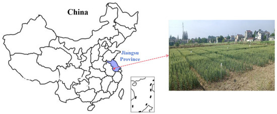
Figure 1.
Experimental site and environment.
2.2. Experimental Data Collection
The experiment utilized a DJI Martrice 300RTK® (Shenzhen DJI Technology Co., Ltd., Shenzhen City, China) quadcopter drone as the flight platform, equipped with an FS60-C® hyperspectral imager (Zhejiang CHNSpec Technology Co., Ltd., Zhejiang City, China). The FS60-C can collect information from 391.43 to 1009.56 nm across 300 spectral bands, with a spectral resolution of 2.5 nm. To facilitate distinction and sampling, the experimental field was divided into 15 experimental zones. Within the 15 experimental zones, 3 sampling zones were set up in each zone, a total of 45 sampling zones, as shown in Figure 2. The sampling zones were all selected in the middle regions of the corresponding experimental zone where the growth was uniform. The size of each sampling zone was 1.5 m by 1.5 m. Sampling took place across four growth stages of wheat, with a total of six sampling events: the jointing stage (29 March and 10 April 2024), the heading stage (18 April and 24 April 2024), the flowering stage (1 May 2024), and the grain filling stage (10 May 2024). To minimize interference from meteorological and environmental factors, all hyperspectral data were collected under conditions of sufficient sunlight and no wind or clouds. The specific collection time was between 10:00 and 14:00, with a flight altitude set at 40 m and a side overlap rate of 60%. Before each flight, the hyperspectral camera undergoes whiteboard calibration. After obtaining the hyperspectral images, the original spectral images were first corrected for reflectance using FigSpecStudio 2.0, provided by the imaging instrument manufacturer. Then, using ENVI 5.6 + IDL (Exelis Visual Information Solutions, Inc., Boulder, CO, USA), a mask was generated through the excess green index (ExG) to eliminate the influence of non-wheat pixels on the spectral data. Finally, the spectral reflectance data of each sampling area was extracted based on the ground markers, and the average was taken to obtain the spectral data of that sampling area.
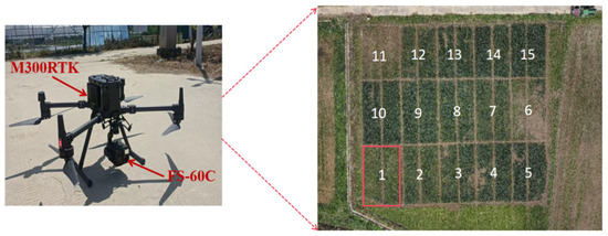
Figure 2.
DJI M300RTK UAV and the division of 15 sampling areas in the experimental zone.
In each sampling, three wheat plants were selected from 45 sampling areas to form one composite sample. During the whole experiment, a total of 270 samples were collected from 6 samplings. The plant samples were taken back to the laboratory for stem and leaf separation, and then the leaf fresh weight (W) of each sample was measured. After that, the samples were blanched for 30 min by 105 °C oven and dried to constant weight by continuous heating at 75 °C, and the dry weight (M) of each sample was measured. Finally, the absolute water content V of each sample was calculated, as shown in Formula (1). Take the average of the LWC of the three wheat samples in each sampling zone, and this average value represented the LWC of that sampling zone.
2.3. Hyperspectral Image Transformation
During outdoor remote hyperspectral sampling, interference from environmental factors such as weather and stray light may occur, which can affect the accuracy of spectral data. Specific spectral transformations can improve the signal-to-noise ratio, making the preprocessed spectral data more sensitive to wheat LWC [24]. In this study, several spectral preprocessing methods were applied to the raw spectra, resulting in six transformed spectra datasets: raw spectrum (R), multiple scattering correction (MSC), standard normal variate (SNV), Savitzky–Golay smoothing (SG), wavelet transform (WT), and first derivative (FD). MSC can effectively correct baseline drift, mitigate noise interference caused by scattering, and enhance the signal-to-noise ratio [25]. SNV can weaken the spectral baseline drift and multiplicative scattering effect caused by the physical properties of wheat, so that the spectral data are more concentrated on reflecting the chemical information of the sample and enhancing the comparability between the spectra [26]. SG smoothing can improve the accuracy and robustness of subsequent modeling by reducing noise while retaining spectral features. WT can simultaneously retain high-frequency and low-frequency spectral information, which is beneficial for eliminating outliers in hyperspectral remote sensing images. FD can highlight the varying components of spectral signals, effectively improving baseline drift issues and minimizing noise interference [27].
2.4. Extraction of Feature Band
Hyperspectral data contains a large number of spectral bands with significant redundancy and interference. Therefore, extracting feature bands relevant to wheat LWC from this vast spectral dataset is of critical importance. This study used competitive adaptive reweighted sampling (CARS) and Hilbert–Schmidt Independence Criterion Lasso (HSICLasso) algorithms as feature band extraction algorithms for wheat hyperspectral data. CARS is a feature variable selection method based on Darwin’s “survival of the fittest” principle. It combines Monte Carlo sampling and partial least squares (PLS) regression coefficients to mimic the process of natural selection, gradually eliminating redundant variables [28]. HSICLasso is a nonlinear feature selection method that effectively identifies the most relevant feature subset from high-dimensional features by combining kernel functions with L1 regularization [29].
2.5. Machine Learning Modeling
After spectral transformation and feature band extraction of hyperspectral data, three machine learning regression algorithms—partial least squares regression (PLSR), support vector regression (SVR), and random forest (RF)—were used to construct estimation models for winter wheat LWC. PLSR is a robust multivariate statistical modeling technique particularly suitable for scenarios involving numerous highly correlated predictor variables, while effectively mitigating noise interference during information extraction [30]. During training, PLSR requires continuous optimization of the number of principal components (n_components). In this study, n_components varied between 5 and 20 (number of spectral bands). SVR is a powerful regression method based on support vector machines. Its kernel trick endows SVR with strong nonlinear modeling capabilities and enhanced robustness [31]. In this study, the kernel function of the SVR model is radial basis function (RBF), and its penalty coefficient (C) is randomly sampled from a log-uniform distribution between (1 × 10⁻², 1 × 10³). RF is a robust and flexible regression modeling tool that enhances prediction stability and accuracy of a single tree by aggregating numerous randomized regression trees. In this study, the number of RF regression trees (n_estimators) ranged from 50 to 150, the maximum depth of a single regression tree (max_depth) varied between 10 and 20, the minimum number of samples per leaf node ranged from 5 to 10, and the minimum number of samples required for node splitting ranged from 10 to 15. The hyperparameters of the above machine learning methods used in this study are detailed in Table 1.

Table 1.
Details of machine learning model methods.
2.6. Machine Evaluation Methods
All models in this study were implemented using either PyTorch 1.13 or scikit-learn 1.2.2 frameworks, with the data processing and experimental procedures illustrated in Figure 3. First, the dataset was randomly split into a training set and a test set in an 8:2 ratio. Second, the spectral transformation was applied to both the training set and the test set. Third, feature selection was performed on the training set data, and the results of the feature selection were applied to the test set. Fourth, the training set data after spectral transformation and feature selection were input into the machine learning model for training, and the corresponding model was obtained. Finally, the test set data was input into the model for prediction, and the model performance was evaluated based on the prediction results. In steps two and three, the training set and test set were processed separately to prevent data leakage.
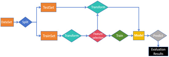
Figure 3.
The data preprocessing and experimental procedure diagram for all the model evaluation methods.
Due to the limited number of samples (270 in total), 50 experiments were conducted for each combination of spectral transformation, feature extraction, and machine learning model to minimize the results randomness caused by the small sample size. For each experiment, the dataset was randomly partitioned. Additionally, all constructed models employed cross-validation to prevent overfitting caused by small datasets.
This study employed the coefficient of determination (R2), mean absolute error (MAE), root mean square error (RMSE), and relative percent difference (RPD) as evaluation metrics to assess model performance [32]. R2 was used to measure the degree of variability of the dependent variable of the model, with values closer to 1 indicating better model fit. MAE represented the average absolute difference between the predicted value and the actual value, ranging from 0 to positive infinity, where smaller values indicate higher prediction accuracy. RMSE measured the root mean square difference between predicted values and actual values. A smaller RMSE indicated higher prediction accuracy and closer alignment with the actual values. RPD represented the ratio of the model’s prediction accuracy to the standard deviation of actual values. A larger RPD value indicated smaller model errors, with RPD > 2 suggesting excellent predictive capability [33].
The evaluation metrics were shown in Formulas (2)–(5): where n represented the sample size; y represented the true value of wheat LWC; represented the model-predicted value of wheat LWC; and represented the average true value of wheat LWC.
3. Results and Analysis
3.1. Wheat Hyperspectral Features Analysis
3.1.1. Hyperspectral Transformation Results
Figure 4 shows the raw spectral curve of winter wheat collected in this paper and the spectral curve after five spectral transformations. As evident in Figure 4A, significant variations exist in the raw reflectance among experimental samples, particularly at wavelengths beyond 700 nm, where distinct reflectance differences emerge between samples. Additionally, the spectral curves exhibit noticeable baseline shifts and jitter phenomena (the jitter phenomena were later found to potentially be related to the hyperspectral lens used for data collection). After MSC (Figure 4B) and SNV (Figure 4C) spectral transformation, a large amount of noise was effectively eliminated, and the phenomenon of baseline shift was also significantly improved. Although there was still a certain jitter in the reflectivity when the wavelength was greater than 900 nm, the reflectivity difference in some characteristic wavelengths was obviously highlighted. The spectral curve after SG smoothing (Figure 4D) significantly eliminated some spikes and noise, but the baseline shifts and slopes between spectra remained unchanged. In contrast, the spectral curve after WT transformation (Figure 4E) demonstrated negligible improvement over the raw spectra, retaining substantial noise and baseline shift. Comparatively, the FD transformation (Figure 4F) highlighted the differences in spectral variations, significantly amplifying the positions of reflectance fluctuation spectra and improving the efficiency of feature band extraction. However, some spikes and jitter phenomena still existed in the wavelength region above 900 nm in Figure 4F, attributable to the strength of the spectral signal and lens factors.
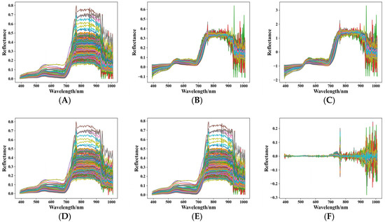
Figure 4.
The raw and transformed spectra curve of wheat. Different colors represented the spectral curves of different samples. Each figure contained 270 colored lines, displayed in a cycle of 10 colors: blue, orange, green, red, purple, brown, etc. (A) Raw spectra, (B) multiple scattering correction transformation spectra, (C) standard normal variate transformation spectra, (D) Savitzky–Golay smoothing transformation spectra, (E) wavelet transformation spectra, (F) first derivative transformation spectra.
3.1.2. Correlation Analysis of Spectral Reflectance and LWC
Based on measured data, the Pearson correlation coefficients between the reflectance of each band and LWC before and after the spectral transformation were calculated. As shown in Formula (6), where n represented the number of samples; x represented the band reflectance; y represented the true value of wheat LWC; represented the average emissivity of the band; represented the average true value of wheat LWC; and r represented the Pearson correlation coefficient. The larger the absolute value of r, the stronger the correlation.
The correlation between band reflectance and LWC before and after hyperspectral transformation is shown in Figure 5. As observed in Figure 5A, the correlation coefficients between the raw hyperspectral bands and LWC range from −0.14 to 0.10, indicating a weak correlation. After MSC (Figure 5B) and SNV (Figure 5C) processing, the MSC-r ranged from −0.47 to 0.34, and the SNV-r ranged from −0.45 to 0.34. The trends in the correlation coefficients between the bands and LWC after the two transformations were similar. The correlation coefficients fluctuated significantly around 900 nm, which better reveals the correlation. In contrast, the correlation curves after SG (Figure 5D) and WT (Figure 5E) processing exhibited no obvious fluctuations, indicating a weak correlation. After FD transformation (Figure 5F), although the fluctuation degree of the correlation coefficient was slower than that of MSC-r and SNV-r, the fluctuation degree of FD-r was obviously enlarged to between −0.63 and 0.49.
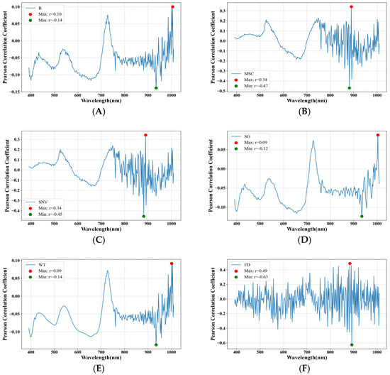
Figure 5.
Correlation analysis of wheat LWC with different transformed spectra. (A) R-r, (B) MSC-r, (C) SNV-r, (D) SG-r, (E) WT-r, (F) FD-r.
Subsequent experiments utilized R, MSC, SNV, and FD spectral data for further analysis.
3.2. Wheat LWC Estimation Models
In this study, three machine learning methods, PLSR, SVR, and RF, were used to construct the evaluation model of wheat LWC. Data from four growth stages of wheat obtained through six samplings were used as an experimental dataset (270 entries), and 80% of the data (216 entries) were randomly selected as the training set to construct the model. Due to the small sample size, to avoid the randomness associated with random sampling during model development, each model was constructed 50 times, with the training dataset being randomly resampled before each construction. Figure 6 shows the evaluation results of three machine learning models combined with different preprocessing methods, with each evaluation metric representing the average of 50 model constructions. The evaluation results of the PLSR, SVR, and RF models are represented by black, red, and blue, respectively. Figure 6A–D shows the R2, MAE, RMSE, and RPD evaluation metrics of the three models, respectively.
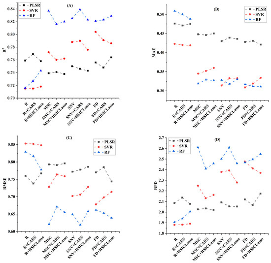
Figure 6.
Comparison of the estimation accuracy of wheat LWC by the combination of three machine learning models and different preprocessing. (A) R2, (B) MAE, (C) RMSE, (D) RPD.
For the PLSR model (black), an analysis was first conducted from the perspective of spectral transformation. When evaluating R, R + CARS, and R + HSICLasso, the PLSR model underperformed the SVR model only in the MAE metric but outperformed other models in terms of R2, RMSE, and RPD. Notably, the evaluation accuracy of the PLSR model even decreased when compared to data processed with MSC, SNV, and FD spectral transformations. Secondly, from the perspective of CARS and HSICLasso feature extraction methods, the PLSR model had no obvious change in the evaluation accuracy when evaluating the data of the same spectral transformation but different feature extraction methods. Notably, on both MSC and SNV datasets, the PLSR model showed decreased evaluation metrics after applying either feature extraction method. However, R + CARS and FD + HSICLasso demonstrated favorable sensitivity responses, with both showing improved evaluation accuracy. The best overall performance was achieved by the FD + HSICLasso + PLSR model, with R2, MAE, RMSE, and RPD metrics reaching 0.764, 0.421, 0.744, and 2.174, respectively.
For the SVR model (red), an analysis was first conducted from the perspective of spectral transformation. After processing with MSC, SNV, and FD transformations, the SVR model exhibited progressively improved evaluation accuracy, with the FD-processed data demonstrating the best performance. Additionally, the RBF kernel function of the SVR model was sensitive to high-frequency changes. As shown in Figure 4F, the spectra processed by FD exhibited high-frequency and high-gradient abrupt changes at the positions of characteristic peaks, which became significant separation points for the kernel function. Secondly, from the feature extraction perspective, application of both CARS and HSICLasso methods resulted in decreased rather than improved evaluation accuracy for the SVR model. The FD + SVR model had the best comprehensive performance, with R2, MAE, RMSE, and RPD reaching 0.804, 0.309, 0.678, and 2.476, respectively.
For the RF model (blue), an analysis was first conducted from the perspective of spectral transformation. Compared with the raw dataset, the RF model demonstrated significantly improved evaluation accuracy after MSC, SNV, and FD spectral processing. Compared with the PLSR and SVR models, the RF model showed better sensitivity to MSC, SNV, and FD spectral transformations and showed no significant differences among the three spectral transformations. Secondly, from the feature extraction perspective, the evaluation accuracy of the RF model is significantly improved after CARS and HSICLasso feature extraction of R and FD spectral transformation. However, an opposite trend was observed for MSC spectral transformation, where both feature extraction methods led to decreased model performance. The best overall performance was achieved by the SNV + CARS + RF model, with R2, MAE, RMSE, and RPD metrics reaching 0.839, 0.318, 0.619, and 2.609, respectively.
3.3. Wheat LWC Estimation Models Test
To further test the generalization and reliability of the model, the average evaluation results of the test set for each data preprocessing and model combination were calculated for 50 model constructions, as shown in Figure 7.
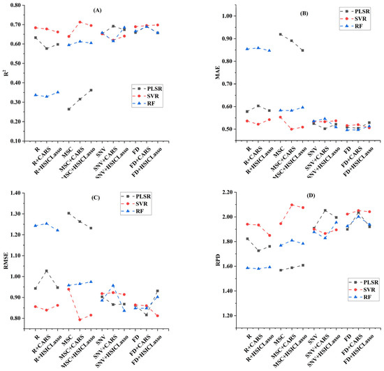
Figure 7.
Comparison of three machine learning models for wheat LWC evaluation on the test set: (A) R2, (B) MAE, (C) RMSE, (D) RPD.
For the PLSR model (black), satisfactory performance was observed on test sets processed with R, SNV, and FD spectral transformations, generally consistent with its training set evaluation results. However, on the MSC test set, the PLSR model had the lowest prediction accuracy among all models, indicating that the MSC + PLSR model combination had poor reliability and even carried certain overfitting risks. Additionally, the performance of the PLSR model on the test set after CARS and HSICLasso feature extraction was the same as that of the training set, with no significant improvement in prediction results. Among all test set evaluations, the SNV + CARS + PLSR combination model achieved the highest prediction accuracy, with R2, MAE, RMSE, and RPD metrics reaching 0.692, 0.502, 0.866, and 2.053, respectively.
The SVR model (red) had high prediction accuracy on the test set for the four spectral transformations of R, MSC, SNV, and FD. The SVR model (red) had high prediction accuracy on the test set for the four spectral transformations of R, MSC, SNV, and FD. From the performance of the test set after feature extraction, the MSC test dataset after CARS and HSICLasso feature extraction on the SVR model had been improved. The prediction accuracy brought by feature extraction had not been significantly improved on other spectral transformation datasets. Overall, the MSC + CARS + SVR combination model achieved the highest prediction accuracy across all test sets, with R2, MAE, RMSE, and RPD metrics reaching 0.713, 0.500, 0.793, and 2.097, respectively.
The RF model (blue) maintained the same trend as the training set in terms of prediction accuracy for the four spectral transformations of R, MSC, SNV, and FD on the test set. But the evaluation results showed a significant decline compared to the training set, especially on the MSC test set. Additionally, from the perspective of CARS and HSICLasso feature extraction, the prediction accuracy on the test set had not been significantly improved. Considering the performance of the RF model across all test sets, the FD + CARS + RF combination model achieved the highest prediction accuracy, with R2, MAE, RMSE, and RPD metrics reaching 0.689, 0.497, 0.848, and 2.002, respectively.
3.4. Model Performance Evaluation
By evaluating the results of the PLSR, SVR, and RF models on training and testing datasets with different spectral processing methods, it could be observed that the RF model achieved the best fitting performance on the training dataset for data after spectral transformation. However, its prediction accuracy significantly decreased on the testing dataset, indicating poorer reliability and stability compared to the PLSR and SVR models. The PLSR model showed poor fitting performance on all training datasets but demonstrated good prediction accuracy on the SNV and FD test datasets. It indicated that the SNV + PLSR and FD + PLSR models exhibited good stability. Finally, although the SVR model performed worse than the RF model on the training set, it demonstrated excellent predictive performance on all test sets. It indicated that the SVR model exhibited better robustness and generalization compared to the PLSR and RF models.
The other three models achieving optimal evaluation performance on the training set were ranked as follows: SNV + CARS + RF, FD + SVR, and FD + HSICLasso + PLSR, while the models achieving best prediction performance on the test set were ranked as follows: MSC + CARS + SVR, SNV + CARS + PLSR, and FD + CARS + RF. This comparative analysis demonstrated that incorporating the CARS feature extraction algorithm significantly enhanced both the predictive accuracy and robustness of the models. Figure 8 shows the best prediction results from the 50 experiments of the three models with the highest prediction accuracy on the test set, as well as the distribution of actual values and predicted values for all samples (54) in the test set. The best prediction results of the MSC + CARS + SVR model are shown in Figure 8A, with R2, MAE, RMSE, and RPD reaching 0.918, 0.347, 0.445, and 3.518, respectively. The best prediction results of the FD + CARS + RF model are shown in Figure 8B, with R2, MAE, RMSE, and RPD reaching 0.892, 0.380, 0.456, and 3.080, respectively. The best prediction results of the SNV + CARS + PLSR model are shown in Figure 8C, with R2, MAE, RMSE, and RPD reaching 0.882, 0.322, 0.440, and 2.937, respectively.

Figure 8.
The model with the best performance in the test set and its prediction results. Different colors represent the Gaussian kernel density estimates of the data points in the space. The redder the color, the more concentrated the data points in that area; the bluer it is, the sparser they are (A) MSC + CARS + SVR, (B) FD + CARS + RF, (C) SNV + CARS + PLSR.
4. Discussion
4.1. The Influence of Spectral Transformation and Feature Selection
Spectral transformations of raw spectral data can improve the quality of spectral data, and the appropriate selection of spectral transformations can effectively enhance the accuracy of spectral analysis results. In this study, six spectral transformations were performed on the hyperspectral data of winter wheat canopy. Based on the spectral transformations and LWC correlation analysis, it was found that neither SG nor WT transformations enhanced the characteristic changes in the reflectance of key spectral bands. In contrast, MSC, SNV, and FD transformations more effectively revealed the relationship between spectral reflectance and wheat LWC. This result was consistent with the results of Guo et al. [4] and Jing et al. [12] in their studies on transformed hyperspectral data of potato and lettuce canopy. Additionally, feature selection could efficiently extract the most representative, stable, and target-property-related set of wavelength features from high-dimensional spectral data [33,34].
The combination effect of different spectral transformations and models was also different. The PLSR model, when evaluating the data after spectral transformation, actually showed a decrease in accuracy. This may be attributed to the fundamental principle of PLSR modeling, which constructed latent variables by maximizing the covariance between spectral reflectance across all bands and LWC. While MSC, SNV, and FD preprocessing can eliminate physical interference and reduce noise, they may also disrupt critical information, thereby affecting the covariance structure and ultimately leading to a decline in the evaluation results of the PLSR model.
The SVR model showed favorable sensitivity to spectral transformations. The reason may be that the kernel function of the SVR model possessed nonlinear modeling capabilities, relying solely on the local relative distances between features. The topological structure of the samples after spectral transformation was more separable in the feature space, which improved the evaluation performance of SVR.
The RF model showed better sensitivity to spectral transformations. The reason may be that the tree splitting mechanism of the RF model directly utilized the preprocessed physical features, and ensemble learning could suppress the side effects of preprocessing, thereby enhancing robustness and maximizing the extraction of feature information from the spectra.
4.2. The Influence of Model Hyperparameter Selection
The selection of hyperparameters in the machine learning model had a great influence on the performance of the final model.
The study first examined the MSC + CARS + SVR model. In the SVR model, the hyperparameter ‘C’ was the regularization parameter, which balanced the model fitting capability and generalization ability. The larger the value of ‘C’, the greater the penalty imposed on errors by the model. The hyperparameter ‘epsilon’ defined the tolerance of the model to prediction errors. The ‘C’ and ‘epsilon’ jointly determined the fitting performance of the SVR model. Figure 9 shows the changes in the MSC + CARS + SVR model with the hyperparameters ‘C’ and ‘epsilon’, and the corresponding model evaluation metrics R2 (Figure 9A) and RPD (Figure 9B). The value of ‘C’ was [0.01, 1, 100, 10,000], and the value of ‘epsilon’ was [0.01, 0.05, 0.1, 0.2, 0.3, 0.5]. When C = 0.01, the model exhibited negative R2 values and RPD approaching 1, regardless of ‘epsilon’ variations, indicating severely poor fitting performance. The model fitting capability progressively improved with increasing C values. When C = 10,000, the model exhibited overfitting, with RPD reaching as high as 13.7 when epsilon = 0.01.
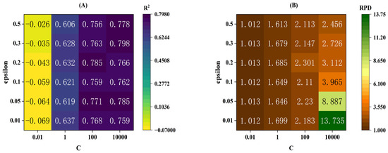
Figure 9.
The changes during the optimization process of hyperparameters C and epsilon of the MSC + CARS + SVR model. (A) R2, (B) RPD.
Next, the SNV + CARS + PLSR model was examined. The core of the number of principal components (n_components) hyperparameters in the PLSR model was to project the raw high-dimensional feature space into the low-dimensional latent variable space, reducing the dimension while retaining the information most relevant to the target variable. If the value of n_components was set too small, it might fail to capture sufficient information. Conversely, an excessively large value could increase computational costs and raise the risk of overfitting, as shown in Figure 10.
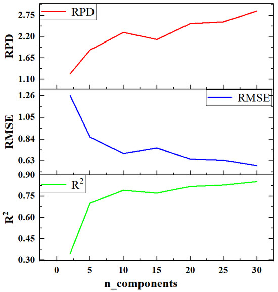
Figure 10.
The changes in R2, RMSE, and RPD during the optimization process of hyperparameters n_components of the SNV + CARS + PLSR model.
In the FD + CARS + RF model, the max_features hyperparameter was used to control the diversity among trees, while the n_estimators hyperparameter enhanced performance by increasing the number of trees. Figure 11 shows the changes in the FD + CARS + RF model with the hyperparameters max_features and n_estimators, and the corresponding model evaluation metrics R2 (Figure 11A) and RMSE (Figure 11B). The value of n_estimators was [50, 60, 70, 80, 100], and the value of max_features was [1.0, ‘sqrt’, ‘log2’], where ‘sqrt’ denoted the square root of the total number of features, and ‘log2’ denoted the logarithm of the total number of features. It could be observed that when max_features = 1, changing the hyperparameter n_estimators caused fluctuations in the evaluation metrics (R2 and RMSE), but the model performance was superior to when max_features = ‘sqrt’ or ‘log2’. However, when max_features = 1 and n_estimators = 100, the model performance showed a significant downward trend. When max_features was set to ‘log2’, the model exhibited the poorest performance on the current dataset, and the performance also showed a decreasing trend as the value of n_estimators increased.
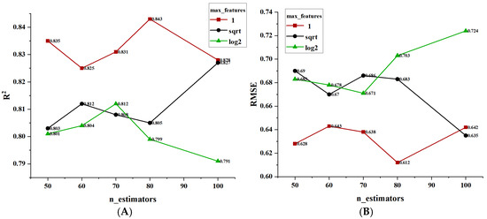
Figure 11.
The changes during the optimization process of hyperparameters max_features and n_estimators of the FD + CARS + RF model. (A) R2, (B) RMSE.
4.3. The Limitations of the Dataset
Although the sample size of this study was only 270, each sample consists of hyperspectral data (with 300 dimensions). First of all, each sample was not a single data point, but rather a complete and continuous spectral “fingerprint” composed of 300 features (spectral reflectance). Therefore, by using machine learning models to learn the patterns in these hyperspectral data, the training foundation was quite solid. Secondly, there was a clear and explainable physical mechanism between the water content of wheat leaves and their spectral reflectance. Water exhibited strong absorption peaks in certain spectral bands [35]. The higher LWC, the more obvious absorption characteristics. Therefore, the evaluation results of the model in this study were based on physical principles. Finally, these 270 samples covered four growth stages. This meant that the 270 samples effectively covered the range that LWC might take on during different growth stages. Therefore, the model in this study learned data that encompassed different growth stages, rather than a locally biased distribution. In conclusion, the dataset of this study can effectively guide the model to achieve an accurate result.
Although the model in this study achieved good evaluation results, it still had certain limitations. For instance, the dataset was collected only from one region for one quarter. The model may not be able to accurately assess the LWC of winter wheat in other regions or under different planting conditions. In the future, we will conduct data sampling of winter wheat in different regions, thereby conducting research on the general applicability of this model.
5. Conclusions
Winter wheat has different water requirements at different growth stages. Rapid measurement of LWC at different growth stages is important for understanding wheat production, formulating irrigation strategies, and field management. In this study, UAV was used as a platform to conduct six canopy hyperspectral data samplings and field measurements of LWC at four growth stages of winter wheat. To improve the quality of the spectral data, six spectral transformations were applied to the hyperspectral data, and correlation analyses were conducted between each spectral transformation and LWC. Ultimately, three transformations—MSC, SNV, and FD—were selected for subsequent research. To eliminate the interference of redundant information in the spectral data, the effects of CARS and HSICLasso feature extraction methods on the model were investigated. Finally, different data preprocessing methods and three machine learning algorithms (PLSR, SVR, RF) were combined to construct a variety of LWC estimation models, and the evaluation results of each model were compared and analyzed. This study drew the following conclusions:
- (1)
- After MSC, SNV, and FD spectral transformation of winter wheat canopy hyperspectral data, the correlation between spectral information and LWC could be significantly improved. Compared with the correlation coefficient of the raw spectral data (−0.14~0.10), the correlation coefficient after MSC, SNV, and FD transformation increased to −0.47~0.34, −0.45~0.34, and −0.63~0.49, respectively.
- (2)
- The CARS and HSICLasso feature extraction methods could effectively remove redundant information from hyperspectral data, improving the prediction accuracy and stability of the model. Notably, based on the test set predictions, the CARS method demonstrated superior performance in enhancing both prediction precision and model stability.
- (3)
- Different models were suited to different data preprocessing methods. The model combinations that performed best on the test set for the three machine learning algorithms were MSC + CARS + SVR, SNV + CARS + PLSR, and FD + CARS + RF. All three models were able to accurately and stably predict winter wheat LWC. Among them, the RF algorithm exhibited superior training data fitting performance and the SVR algorithm showed enhanced robustness and generalization ability.
Author Contributions
Conceptualization, Y.W. and Y.T.; methodology, Y.W. and Y.T.; software, J.Z.; investigation, Y.W.; resources, Y.T.; writing—original draft preparation, Y.W. and L.T.; writing—review and editing, Y.W., S.Y. and L.T.; supervision, S.Y. and Y.T.; project administration, S.Y. and Y.T.; funding acquisition, L.T. All authors have read and agreed to the published version of the manuscript.
Funding
This work was supported by the National Key Research and Development Program of China, grant number 2023YFD1900704.
Institutional Review Board Statement
Not applicable.
Data Availability Statement
The datasets used and/or analyzed during the current study are available from the corresponding author on reasonable request.
Conflicts of Interest
The authors declare no conflicts of interest.
References
- Zhao, H.; Zhang, L.; Kirkham, M.B.; Welch Stephen, M.; Nielsen Gammon John, W.; Bai, G.; Luo, J.; Andresen Daniel, A.; Rice Charles, W.; Wan, N.; et al. U.S. winter wheat yield loss attributed to compound hot-dry-windy events. Nat. Commun. 2022, 131, 7233. [Google Scholar] [CrossRef]
- Wu, Z.; Luo, J.; Rao, K.; Lin, H.; Song, X. Estimation of wheat kernel moisture content based on hyperspectral reflectance and satellite multispectral imagery. Int. J. Appl. Earth Obs. Geoinf. 2024, 126, 103597. [Google Scholar] [CrossRef]
- Zhai, W.; Cheng, Q.; Duan, F.; Huang, X.; Chen, Z. Remote sensing-based analysis of yield and water-fertilizer use efficiency in winter wheat management. Agric. Water Manag. 2025, 311, 109390. [Google Scholar] [CrossRef]
- Guo, F.; Feng, Q.; Yang, S.; Yang, W. Estimation of potato canopy leaf water content in various growth stages using UAV hyperspectral remote sensing and machine learning. Front. Plant Sci. 2024, 15, 1458589. [Google Scholar] [CrossRef]
- Sun, D.; Zhang, L.; Li, H.; Lan, W.; Tu, K.; Liu, J.; Pan, L. Non-destructive prediction of the moisture content of individual wheat kernels combining hyperspectral imaging and WGAN data augmentation algorithm. Food Res. Int. 2025, 212, 116498. [Google Scholar] [CrossRef]
- Katsoulas, N.; Elvanidi, A.; Ferentinos, P.K.; Kacira, M.; Bartzanas, T.; Kittas, C. Crop reflectance monitoring as a tool for water stress detection in greenhouses: A review. Biosyst. Eng. 2016, 151, 374–398. [Google Scholar] [CrossRef]
- Qian, C.; Fan, D.; Honggang, X.; Guo, S.; Li, Z.; Chen, Z. Quantifying corn LAI using machine learning and UAV multispectral imaging. Precis. Agric. 2024, 254, 1777–1799. [Google Scholar] [CrossRef]
- Adak, A.; DeSalvio, J.A.; Murray, C.S. A computational framework for modeling and predicting maize senescence: Integrating UAV phenotyping, logistic growth, and genomics. Comput. Electron. Agric. 2025, 237, 110471. [Google Scholar] [CrossRef]
- Gu, Q.; Huang, F.; Lou, W.; Zhu, Y.; Hu, H.; Zhao, Y. Unmanned aerial vehicle-based assessment of rice leaf chlorophyll content dynamics across genotypes. Comput. Electron. Agric. 2024, 221, 108939. [Google Scholar] [CrossRef]
- Kang, Y.; Wang, Y.; Fan, Y.; Wu, H.; Zhang, Y.; Yuan, B. Wheat Yield Estimation Based on Unmanned Aerial Vehicle Multispectral Images and Texture Feature Indices. Agriculture 2024, 14, 167. [Google Scholar] [CrossRef]
- Yang, N.; Zhang, Z.; Zhang, J.; Yang, X.; Liu, H.; Chen, J. Accurate estimation of winter-wheat leaf water content using continuous wavelet transform-based hyperspectral combined with thermal infrared on a UAV platform. Eur. J. Agron. 2025, 168, 127624. [Google Scholar] [CrossRef]
- Jing, Z.; Hong, L.; Chao, C.; Pang, Y.; Zhu, X. Detection of Water Content in Lettuce Canopies Based on Hyperspectral Imaging Technology under Outdoor Conditions. Agriculture 2022, 12, 1796. [Google Scholar] [CrossRef]
- Gao, C.; Liu, S.; Wu, P.; Wu, P.; Wang, Y.; Wu, K.; Li, L. Estimation of Canopy Water Content by Integrating Hyperspectral and Thermal Imagery in Winter Wheat Fields. Agronomy 2024, 14, 2569. [Google Scholar] [CrossRef]
- Dong, L.; Weiguo, Y.; Hengbiao, Z.; Guo, C.; Xia, Y.; Yan, Z. Towards practical semi-empirical models for the estimation of leaf and canopy water contents from hyperspectral reflectance. Comput. Electron. Agric. 2023, 214, 108309. [Google Scholar] [CrossRef]
- Ji, J.; Lu, X.; Ma, H.; Jin, X.; Jiang, S.; Cui, H. Estimation of plant leaf water content based on spectroscopy. Front. Plant Sci. 2025, 16, 1609650. [Google Scholar] [CrossRef]
- Junttila, S.; Hölttä, T.; Saarinen, N.; Kankare, V.; Yrttimaa, T.; Hyyppä, J.; Vastaranta, M. Close-range hyperspectral spectroscopy reveals leaf water content dynamics. Remote Sens. Environ. 2022, 277, 113071. [Google Scholar] [CrossRef]
- Li, R.; Yao, F.; Xu, Y.; Bai, S.; Jia, Z.; Lin, Q. Optimizing the Charge Carrier Dynamics of Thermal Evaporated TexSe1-x Films for High-Performance Short-Wavelength Infrared Photodetection. Adv. Funct. Mater. 2023, 34, 2307005. [Google Scholar] [CrossRef]
- Raj, R.; Walker, J.P.; Vinod, V.; Pingale, R.; Naik, B.; Jagarlapudi, A. Leaf water content estimation using top-of-canopy airborne hyperspectral data. Int. J. Appl. Earth Obs. Geoinf. 2021, 102, 102393. [Google Scholar] [CrossRef]
- Kovar, M.; Brestic, M.; Sytar, O.; Barek, V.; Hauptvogel, P.; Zivcak, M. Evaluation of Hyperspectral Reflectance Parameters to Assess the Leaf Water Content in Soybean. Water 2019, 11, 443. [Google Scholar] [CrossRef]
- Clevers, J.G.; Kooistra, L.; Schaepman, M.E. Estimating canopy water content using hyperspectral remote sensing data. Int. J. Appl. Earth Obs. Geoinf. 2010, 12, 119–125. [Google Scholar] [CrossRef]
- Sun, X.; Zhang, B.; Dai, M.; Jing, C.; Ma, K.; Tang, B. Accurate irrigation decision-making of winter wheat at the filling stage based on UAV hyperspectral inversion of leaf water content. Agric. Water Manag. 2024, 306, 109171. [Google Scholar] [CrossRef]
- Zhou, L.; Lin, J.; Wu, J.; Du, R.; Chen, M.; Zhao, B.; Yang, R. Assessing the potential of red solar-induced chlorophyll fluorescence for drought monitoring in different growth stages of winter wheat. Ecol. Metr. 2024, 161, 111960. [Google Scholar] [CrossRef]
- Li, Q.; Gao, M.; Li, Z.L. Ground Hyper-Spectral Remote-Sensing Monitoring of Wheat Water Stress during Different Growing Stages. Agronomy 2022, 12, 2267. [Google Scholar] [CrossRef]
- Yang, C.; Xu, J.; Feng, M.; Bai, J.; Sun, H.; Song, L. Evaluation of Hyperspectral Monitoring Model for Aboveground Dry Biomass of Winter Wheat by Using Multiple Factors. Agronomy 2023, 13, 983. [Google Scholar] [CrossRef]
- Ruiyan, C.; JunMeng, L.; Yan, W.; Shiyan, F.; Keqiang, Y.; Yanru, Z. Hyperspectral imaging coupled with Dual-channel convolutional neural network for early detection of apple valsa canker. Comput. Electron. Agric. 2022, 202, 107411. [Google Scholar] [CrossRef]
- Qi, H.; Chen, A.; Yang, X.; Xing, X. Estimation of crude protein content in natural pasture grass using unmanned aerial vehicle hyperspectral data. Comput. Electron. Agric. 2025, 229, 109714. [Google Scholar] [CrossRef]
- Chen, X.; Li, F.; Chang, Q.; Miao, Y.; Yu, K. Improving winter wheat plant nitrogen concentration prediction by combining proximal hyperspectral sensing and weather information with machine learning. Comput. Electron. Agric. 2025, 232, 110072. [Google Scholar] [CrossRef]
- Wang, C.; Fu, X.; Zhou, Y.; Fu, F. Deoxynivalenol Detection beyond the Limit in Wheat Flour Based on the Fluorescence Hyperspectral Imaging Technique. Foods 2024, 13, 897. [Google Scholar] [CrossRef] [PubMed]
- Mingzhu, T.; Yutao, C.; Huawei, W.; Qi, Z.; Wen, L.; Victor, S.; Jiabiao, Y. Cost-Sensitive Extremely Randomized Trees Algorithm for Online Fault Detection of Wind Turbine Generators. Front. Energy Res. 2021, 9, 2307005. [Google Scholar] [CrossRef]
- Adesokan, M.; Alamu, O.E.; Otegbayo, B.; Asfaw, A.; Afolabi, M.O.; Fawole, S. Rapid analysis of starch, sugar, and amylose in fresh yam tubers and boiled yam texture using near-infrared hyperspectral imaging and chemometrics. J. Food Compos. Anal. 2025, 142, 107425. [Google Scholar] [CrossRef]
- Shu, M.; Zhu, J.; Yang, X.; Gu, X.; Li, B.; Ma, Y. A spectral decomposition method for estimating the leaf nitrogen status of maize by UAV-based hyperspectral imaging. Comput. Electron. Agric. 2023, 212, 108100. [Google Scholar] [CrossRef]
- Wali, K.; Khan, A.H.; Sica, P.; Henten, E.; Meers, E.; Brunn, S. Application of fourier transform infrared photoacoustic spectroscopy for quantification of nutrient contents and their plant availability in manure and digestate. Heliyon 2024, 10, e28487. [Google Scholar] [CrossRef]
- Wang, X.; Xu, H.; Zhou, J.; Fang, X.; Shuai, S.; Yang, X. Analysis of Vegetation Canopy Spectral Features and Species Discrimination in Reclamation Mining Area Using In Situ Hyperspectral Data. Remote Sens. 2024, 16, 2372. [Google Scholar] [CrossRef]
- Hou, K.; Bai, T.; Li, X.; Shi, Z.; Li, S. Inversion Study of Nitrogen Content of Hyperspectral Apple Canopy Leaves Using Optimized Least Squares Support Vector Machine Approach. Forests 2024, 15, 268. [Google Scholar] [CrossRef]
- Crusiol, L.G.T.; Nanni, M.R.; Furlanetto, R.H.; Sibaldelli, R.N.R.; Sun, L.; Gonçalves, S.L.; Foloni, J.S.S.; Mertz-Henning, L.M.; Nepomuceno, A.L.; Neumaier, N.; et al. Assessing the sensitive spectral bands for soybean water status monitoring and soil moisture prediction using leaf-based hyperspectral reflectance. Agric. Water Manag. 2023, 277, 108089. [Google Scholar] [CrossRef]
Disclaimer/Publisher’s Note: The statements, opinions and data contained in all publications are solely those of the individual author(s) and contributor(s) and not of MDPI and/or the editor(s). MDPI and/or the editor(s) disclaim responsibility for any injury to people or property resulting from any ideas, methods, instructions or products referred to in the content. |
© 2025 by the authors. Licensee MDPI, Basel, Switzerland. This article is an open access article distributed under the terms and conditions of the Creative Commons Attribution (CC BY) license (https://creativecommons.org/licenses/by/4.0/).