Article

Analyzing Spatiotemporal Variations and Influencing Factors in Low-Carbon Green Agriculture Development: Empirical Evidence from 30 Chinese Districts

1
College of Agriculture, Guangxi University, Nanning 530004, China
2
College of Economics and Management, Fujian Agriculture and Forestry University, Fuzhou 350002, China
*
Author to whom correspondence should be addressed.
Agriculture 2025, 15(17), 1853; https://doi.org/10.3390/agriculture15171853 (registering DOI)
Submission received: 27 July 2025 / Revised: 28 August 2025 / Accepted: 28 August 2025 / Published: 30 August 2025
(This article belongs to the Section Agricultural Economics, Policies and Rural Management)

Abstract

Agriculture is fundamental to food security and environmental sustainability. Advancing its holistic ecological transformation can stimulate socioeconomic progress while fostering human–nature harmony. Utilizing provincial data from mainland China (2013–2022), this research establishes a multidimensional evaluation framework across four pillars: agricultural ecology, low-carbon practices, modernization, and productivity enhancement. Through comprehensive assessment, we quantify China’s low-carbon green agriculture (LGA) development trajectory and conduct comparative regional analysis across eastern, central, and western zones. As for methods, this study employs multiple econometric approaches: LGA was quantified using the TOPSIS entropy weight method at the first step. Moreover, multidimensional spatial–temporal patterns were characterized through ArcGIS spatial analysis, Dagum Gini coefficient decomposition, Kernel density estimation, and Markov chain techniques, revealing regional disparities, evolutionary trajectories, and state transition dynamics. Last but not least, Tobit regression modeling identified driving mechanisms, informing improvement strategies derived from empirical evidence. The key findings reveal the following: 1. From 2013 to 2022, LGA in China fluctuated significantly. However, the current growth rate is basically maintained between 0% and 10%. Meanwhile, LGA in the vast majority of provinces exceeds 0.3705, indicating that LGA in China is currently in a stable growth period. 2. After 2016, the growth momentum in the central and western regions continued. The growth rate peaked in 2020, with some provinces having a growth rate exceeding 20%. Then the growth rate slowed down, and the intra-regional differences in all regions remained stable at around 0.11. 3. Inter-regional differences are the main factor causing the differences in national LGA, with contribution rates ranging from 67.14% to 74.86%. 4. LGA has the characteristic of polarization. Some regions have developed rapidly, while others have lagged behind. At the end of our ten-year study period, LGA in Yunnan, Guizhou and Shanxi was still below 0.2430, remaining in the low-level range. 5. In the long term, the possibility of improvement in LGA in various regions of China is relatively high, but there is a possibility of maintaining the status quo or “deteriorating”. Even provinces with a high level of LGA may be downgraded, with possibilities ranging from 1.69% to 4.55%. 6. The analysis of driving factors indicates that the level of economic development has a significant positive impact on the level of urban development, while the influences of urbanization, agricultural scale operation, technological input, and industrialization level on the level of urban development show significant regional heterogeneity. In summary, during the period from 2013 to 2022, although China’s LGA showed polarization and experienced ups and downs, it generally entered a period of stable growth. Among them, the inter-regional differences were the main cause of the unbalanced development across the country, but there was also a risk of stagnation and decline. Economic development was the general driving force, while other driving factors showed significant regional heterogeneity. Finally, suggestions such as differentiated development strategies, regional cooperation and resource sharing, and coordinated policy allocation were put forward for the development of LGA. This research is conducive to providing references for future LGA, offering policy inspirations for LGA in other countries and regions, and also providing new empirical results for the academic community.

1. Introduction

Climate–environmental degradation jeopardizes human–nature coexistence. Since the 1987 formalization of sustainable development, carbon reduction and green transition have gained global priority. FAO data indicates agricultural activities and land-use changes contribute ≈25% to anthropogenic emissions, solidifying low-carbon green agriculture (LGA) as an international imperative [1]. China’s agricultural sector constitutes a vital economic pillar, and it is one of the largest developing economies. Its prolonged dependence on high-input, high-output production models, however, undermines agricultural sustainability [2]. In this context, advancing LGA constitutes an imperative developmental pathway for China and the world. Defined as an agricultural system characterized by minimal emissions, energy efficiency, and high productivity, LGA pursues sustainable agriculture through concurrent emissions reduction, energy conservation, and livelihood enhancement [3,4,5,6]. Similarly to most developing countries, China experiences regional developmental disparities due to divergent economic conditions and resource distribution.
Leveraging 2013–2022 provincial data from mainland China, this study constructs an objective comprehensive evaluation system, and systematically analyzes the dynamic spatial–temporal evolution, regional differences, sources, and driving factors of China’s LGA by using a variety of measurement methods. Initial phase: Integrating the ecological civilization framework and Rural Revitalization Strategy backdrop, we examine contemporary development patterns using foundational theories. Provincial panel datasets (2013–2022) are analyzed through the TOPSIS entropy weighting method to quantify LGA performance levels. Spatial assessment phase: ArcGIS-based cartographic visualization stratifies evaluation outcomes across eastern, central, and western macro-regions. Regional disparity structures are quantified via Dagum Gini coefficient decomposition, capturing intra/inter-regional differentials. Dynamic analysis phase: Nationwide and region-specific LGA evolution trajectories are characterized through non-parametric Kernel density estimation; spatial autocorrelation diagnostics coupled with Markov chain probability modeling project transitional tendencies. Final phase: Multivariate drivers are investigated using censored Tobit regression modeling.
Under such a major premise, the purposes of conducting this study are as follows:
  • To construct a comprehensive evaluation framework for low-carbon green agriculture (LGA) that captures both spatial heterogeneity and temporal dynamics, addressing gaps in existing methodologies;
  • To empirically examine the spatiotemporal evolution of LGA development across 30 representative districts in China, providing replicable analytical pathways for similar developing economies;
  • To identify and quantify the key socioeconomic and environmental drivers influencing LGA disparities, thereby advancing theoretical understandings of LGA’s transitions in resource-constrained contexts.
This investigation centers on decadal (2013–2022) agricultural green–low-carbon development trajectories across China’s 30 provincial units, with the primary objective of formulating a multidimensional, scientifically rigorous, and operationally adaptable LGA assessment framework specifically designed for resource-constrained developing economies. The resultant benchmarking system provides critical methodological reference points for quantitatively evaluating agroecological modernization processes. Concurrently, the study addresses persistent methodological gaps in the extant literature through enhanced data contemporaneity and expanded geographical granularity, thereby furnishing the academic community with temporally comprehensive and spatially exhaustive empirical evidence. Secondly, this research’s results can serve as an important information tool for monitoring LGA, and this evaluation system conducts comprehensive evaluations from four dimensions: greening, low-carbon, modernization, and high efficiency. It helps identify problems in the process of agricultural development and provides a scientific theoretical basis for governments at all levels to formulate agricultural development plans, ecological environment protection, and human settlement environment improvement policies. According to the empirical results of the overall level and driving factors, we will comprehensively grasp the current situation of LGA in China, propose differentiated policy recommendations for regions with different development levels, promote the development of LGA, achieve sustainable agricultural development, and provide development ideas and experience for other countries and regions in the world.

2. Literature Review and Technical Route

2.1. Literature Review

Low-carbon green agriculture (LGA) is a new agricultural production concept that balances ecology and economy. It is the advanced stage of agricultural development, closely related to regional development, relying on the support of the social economy, emphasizing air and environmental health as well as the efficient use of land resources to promote sustainable and intensive development [7,8,9]. As an emergent conceptual paradigm, this approach was originally conceptualized within the taxonomic frameworks of sustainable agriculture and organic farming systems. It constitutes an integrated context-sensitive production framework that prioritizes the implementation of locally adapted management protocols to holistically enhance the structural and functional integrity of agroecosystems, while sustainable agriculture is an agricultural system that can promote and enhance agricultural efficiency, agricultural ecosystems, and local communities (and their development) [10]. With the proposal of a low-carbon economy, People are paying more and more attention to LGA, a production concept that is more in line with the modern social economy [11]. In recent years, reports on LGA have mainly focused on the influence mechanisms of other objective factors on LGA and the interaction mechanisms between the two. One study constructed a three-party game model and found that appropriate carbon trading prices and subsidies can promote farmers to engage in green planting, and that consumers’ green consumption behavior is related to the utility obtained from purchasing green agricultural products [12]. The entropy method was applied to measure the level of development of green and low-carbon agriculture, and combined with the Spatial Error Model (SEM) and Mediation Effect Model, it was concluded that digital inclusive finance not only promotes the development of green and low-carbon agriculture in China, but also has spatial spillover effects [13]. In another study, the conclusion was drawn that green and low-carbon agricultural production in ethnic minority areas can promote household income, based on data obtained through field investigations and analyzed using the OLS (Ordinary Least Squares) regression method [14]. Scientists have used the Super SBM Undesirable Model combined with logit regression to conclude that cooperative management enhances the ecological efficiency of farmland utilization by increasing farmers’ willingness for green development. The stronger the willingness for green development, the more likely farmers are to adopt green innovation [15]. In China’s greenhouse gas emissions, the greenhouse gas intensity of wheat and corn is higher in the north, while that of rice is higher in the southeast [16]. The digital economy is strongly correlated with the green development of agriculture and has a significant nonlinear trend [17,18]. In Chengdu, China, the green development of agriculture is highly coupled with the development of park cities, and the degree of coupling between the two sides has a strong positive spatial correlation [19]; the application of the two-way fixed effects model has empirically tested that the protection of agricultural heritage sites positively promotes green agricultural development and has heterogeneity [20]. In terms of the evaluation system, researchers tends to evaluate LGA from multiple perspectives such as environmental ecology [13], agricultural policy [21] and low-carbon agriculture [22]. At the same time, the selection of research methods is also very diverse: researchers have studied related low-carbon and green agriculture using super slacks-based measure (SBM) models [23,24], and similar DEA models [25,26], while life cycle assessment (LCA) [27], the entropy weight method [28], TOPSIS models [29], the CRITIC entropy approach [30], and analytic hierarchy process also play roles in this field [31]. In addition, some studies combine multiple research methods. For instance, by establishing a comprehensive assessment model and combining the entropy method with the gray relational degree, the overall effect of regional low-carbon development can be accurately evaluated [32,33]. By integrating the difference-in-differences (DID) econometric framework with the spatial Durbin model in a unified analytical design, researchers have rigorously evaluated both the realized effectiveness and the spatially mediated ripple effects of low-carbon development policies, thereby illuminating the conspicuous disparities in green and low-carbon advancement levels across diverse geographical units and offering an in-depth exploration of the underlying determinants that may account for such heterogeneous outcomes [34]. Meanwhile, The Isomap algorithm, Ant Colony Optimization algorithm—commonly abbreviated as ACO—as well as Extremely Randomized Trees regressor, known as ET, have been adopted to optimize the predictive ability of evaluation models [35], while GIS as well as life cycle inventory methodology were employed in the domain of LGA [36]. Even though there are many reports related to LGA at present, in terms of constructing the evaluation index system, scientists have mainly focused on one aspect of LGA, namely its ecological friendliness, low emissions, and low cost. For the other aspect of LGA, the attention to high efficiency, such as the mechanization that should be included in agricultural modernization, is not comprehensive enough, and should also consider the energy consumption of diesel, carbon emissions, and agricultural machinery power simultaneously and comprehensively. In addition, the agricultural, forestry, animal husbandry, and fishery service industries, which integrate technology, logistics, finance, and ecological resources, are important parts of the modernization of LGA, but the existing evaluation systems rarely take them into consideration [37,38,39]. Some have a relatively narrow scope [19,40], and others focus on the impact and mechanisms of LGA and other influencing factors, with insufficient attention paid to the sources, evolutionary trends, and future development of LGA differences [41,42,43]. The contribution of this paper lies in first providing a new paradigm for the evaluation of LGA, second offering new empirical data for LGA research, and third offering more appropriate development suggestions based on the research results.

2.2. Technical Route

This study focuses on LGA in China, systematically exploring its current level, evolution trajectory, influencing factors, and optimization paths under the background of ecological civilization construction and the “dual carbon” strategy. The research follows the logic of “development–evolution–attribution–countermeasures”, and constructs a progressive framework of “macro evaluation–spatiotemporal characterization–mechanism identification–path design”, aiming to clarify the historical position, stage characteristics, spatial pattern, and future trends of China’s LGA, and provide targeted, operational and strategic policy references for China’s LGA and its modernization and agricultural quality across nations (Figure 1). The specific procedures are as follows:
  • Elaborate on the urgency and significance of this research under global climate governance and the “dual carbon” goals and review the research progress, debates, and practices of LGA, pointing out the deficiencies in the spatiotemporal scale, mechanism identification, and policy integration of existing studies. Make the research objectives, ideas, and methods clear (TOPSIS entropy weighting method, Dagum Gini coefficient, Kernel density estimation calculation, spatial autocorrelation analysis, Markov chains, and Tobit regression model).
  • Development Level Quantification Framework: Methodologically formulated around the core tenets of “ecological sustainability, carbon mitigation, operational efficiency, and production modernization,” a multidimensional assessment architecture is constructed. This framework encompasses four pivotal advancement domains—agroecological resilience, agricultural decarbonization pathways, modernization of farming systems, and productivity enhancement mechanisms—operationalized through 15 granular metrics.
  • Empirical Implementation: Leveraging longitudinal provincial datasets (2013–2022) spanning 30 Chinese administrative divisions, comprehensive indices are algorithmically derived via the TOPSIS entropy weighting protocol. This computationally rigorous approach delineates the macroevolutionary trajectory of China’s LGA development paradigm.
  • Spatiotemporal Dynamics Investigation: Geospatial patterning is cartographically determined through ArcGIS geostatistical modeling; regional disparity causality is quantitatively decomposed using the Dagum Gini coefficient decomposition technique; distributional evolutionary properties are non-parametrically characterized via Kernel density estimation methodologies. By rigorously constructing and precisely calibrating Markov chains whose transition probabilities are estimated from current empirical data, this study forecasts the probabilistic trajectories of future evolutionary trends and derives the long-run steady-state distributions that these stochastic processes converge toward. Simultaneously, it analyzes the intricate spatial correlations—quantified through carefully designed distance-weighted matrices—among regions situated at distinct hierarchical levels within the LGA framework, thereby furnishing a nuanced and evidence-rich basis upon which targeted, zone-specific policy implementations can be strategically grounded.
  • Research on Driving Factors: Based on the experiences of predecessors and the internal conditions and external environment of LGA, influencing factors are selected from dimensions including economic development, urbanization processes, scale of the agricultural industry, operation, industrial scale, technological development, and industrialization. We analyze the heterogeneity mechanism of each factor in the overall, upper, middle, and lower subsamples, providing evidence for precise policy-making.
  • Enhancement Paths and Policy Recommendations: Starting from “low carbon, environmental protection, and high efficiency”, combined with the results of empirical analysis, and following the logic of “goal–path–policy”, recommendations are made for improving LGA under different conditions.
In conclusion, the key value of this study is in accurately grasping the definition of LGA, constructing a new system for evaluating it, scientifically assessing LGA in China through the TOPSIS entropy weight method, impersonally revealing its actual characteristics, and conducting a visual dynamic empirical analysis from the perspective of the coupling of time and space. Moreover, considering the sensitivity of different regions to different influencing factors, the internal mechanism is analyzed, hoping to maximize the efficiency of policy and resource allocation.

3. Materials and Methods

3.1. Research Object and Data Source

Drawing upon an unbroken, decade-long panel dataset that spans precisely thirty provincial-level administrative units situated across the Chinese mainland and that covers every calendar year from 2013 through 2022, the present investigation—so as to safeguard both the internal consistency of the analytical outputs and the longitudinal comparability of the derived findings—adopts the official regional classification schema promulgated by the National Bureau of Statistics of China. This authoritative schema, which meticulously synthesizes geographical proximity, macroeconomic performance, and socio-demographic characteristics into a coherent tripartite partition, leads to the delineation of three macro-regional analytical domains, each subsequently subjected to rigorous comparative scrutiny: the eastern macro-region, the central macro-region, and the western macro-region [44]. Within this three-tier regional architecture, the eastern macro-region is explicitly constituted by the eleven provincial-level jurisdictions of Beijing, Tianjin, Hebei, Liaoning, Shanghai, Jiangsu, Zhejiang, Fujian, Shandong, Guangdong, and Hainan, each of which is situated along or proximate to the nation’s coast and is characterized by advanced industrial structures and high degrees of openness. The central macro-region, serving as a transitional belt between the prosperous east and the developing west, comprises nine administrative units—namely, Shanxi, Inner Mongolia, Jilin, Heilongjiang, Anhui, Jiangxi, Henan, Hubei, and Hunan—whose geographical centrality, resource endowments, and evolving manufacturing bases collectively define their intermediate developmental status. The western macro-region, by contrast, encompasses ten provincial-level entities—Guangxi, Chongqing, Sichuan, Guizhou, Yunnan, Shaanxi, Gansu, Qinghai, Ningxia, and Xinjiang—spanning vast land areas marked by complex topography, significant ethnic diversity, and strategic importance for national ecological security and resource supply.
To safeguard the scientific integrity, empirical robustness, and policy applicability of the ensuing analyses, every stage of data selection and processing is executed under a stringent quality-control protocol that systematically screens for missing observations, harmonizes indicator definitions, and reconciles temporal discrepancies. The primary quantitative sources feeding this protocol are the complete historical editions—covering the identical 2013–2022 timeframe—of four flagship annual compendiums issued by the National Bureau of Statistics of China [45] and its specialized affiliates—the China Statistical Yearbook [46], the China Population and Employment Statistical Yearbook [47], the China Rural Statistical Yearbook [48], and the China Science and Technology Statistical Yearbook [49]—and individual provincial statistical yearbooks and related datasets like Wind Information [50].

3.2. LGA Evaluation Index System Construction

LGA includes low-carbon and green agriculture. Low-carbon refers to lower direct greenhouse gas emissions, while green emphasizes ecological friendliness and less pollution from external materials and chemicals [51,52]. LGA, as a modern agricultural model, emphasizes carbon emissions from the production process, organic and recyclable yet pollution-free production materials, and highly efficient production methods [53]. Based on this, this study takes the principles of scientific nature, systematic nature, and operability as its foundation; fully refers to the achievements of predecessors; and comprehensively considers factors such as depletion of resources, carbon emissions, efficient use of resources, and ecological environment protection [1,38,39,54,55]. From the perspectives of ecological sustainability and economic efficiency, it takes the four dimensions of agricultural greening, agricultural low-carbonization, agricultural modernization, and agricultural efficiency as the first-level indicators in order to constitute the quadruple core of LGA. Fifteen indicators are regarded as secondary indicators. The meanings, attributes (“+” stands for positive nature, while “−” stands for passive nature), and weights of the indicators are shown below (Table 1). It is worth noting that agricultural carbon emissions may lead to deviations in results due to different calculation methods [56]. Moreover, considering the non-exclusivity of agriculture, we decided to select a regional agricultural carbon emission scale. The two secondary indicators are agricultural carbon emission density and agricultural carbon emission intensity. In addition, in order to solve the problem that the existing LGA evaluation system does not focus on the agriculture, forestry, animal husbandry, and fishery service industries, the socialization of agricultural production was selected as an indicator. The sources of the remaining indicators are detailed in Table 1.
In order to verify the statistical dependence of each index in the LGA evaluation system, this paper uses the Spearman rank correlation coefficient to test the correlation among each index [64]. The results show (Table S1) that the secondary indicators “Agricultural carbon emission density”, “Agricultural carbon emission intensity”, “Agricultural output level”, and “Socialization of agricultural production” are relevant. Except for the two pairs of indicators, the Spearman rank correlation coefficients among the other indicators were all lower than 0.8, and there was no high correlation. However, in order to ensure the accurate calculation of agricultural carbon emissions and take into account the irreplaceable agricultural, forestry, animal husbandry, and fishery services of modern LGA. Therefore, this study decided to remove the respective strongly correlated indicators to verify its robustness, with a total of four groups in pairs. We recalculated and conducted the Spearman rank correlation coefficient test on the calculated rankings and scores to ensure the robustness of the measurement results. The results show (Table S2) that the Spearman coefficients of the calculation results and rankings before and after removal are all beyond 0.8, and at the 1% level, it proves that although there is a correlation in some individual indicators, this has little impact on the final evaluation result. In addition, the weight size changes little (as shown in Tables S3–S6). This proves the robustness of the calculation results.

3.3. Methods

3.3.1. TOPSIS Entropy Weight Method

Given that the entropy weighting methodology inherently determines objective weighting coefficients commensurate with the relative informational value extracted from indicator variability in observed data, it functionally mitigates potential distortions attributable to subjective determinants inherent in conventional expert-based approaches [65]. The technique for order preference by similarity to ideal solution—commonly abbreviated as the TOPSIS model—stands as a widely embraced, matrix-driven decision-making instrument within the discipline of systems engineering; by quantifying the geometric distances that separate each alternative from both the positive-ideal solution and the negative-ideal solution, the method orchestrates a rigorous, stepwise ranking of alternatives according to their relative proximity to the optimal benchmark, thereby endowing the subsequent analytical conclusions with a demonstrably higher degree of objectivity, transparency, and reproducibility [26]. Therefore, this paper adopts the entropy-augmented TOPSIS methodology to precisely gauge and evaluate LGA across China. The explicit procedural sequence unfolds as follows:
Step 1: Matrix construction: On the basis of every secondary indicator within the established evaluation index system, the original evaluation matrix for LGA in China is defined as
X = x 11 x 12 x 1 n x 21 x 22 x 2 n x m 1 x m 2 x m n
Step 2: Comprehensive standardization of the evaluation matrix. To neutralize the disparate units, scales, and directionalities inherent in the raw data indicators, each element of the initial evaluation matrix is subjected to a rigorous standardization protocol that yields a dimensionally homogeneous intermediate matrix; this intermediate matrix is subsequently refined through a meticulous normalization procedure that rescales every entry into a strictly comparable 0–1 interval. The fully processed, standardized matrix—now purged of any magnitude or polarity distortions—emerges as
R = y 11 y 12 y 1 n y 21 y 22 y 2 n y m 1 y m 2 y m n
Within this context, X denotes the original evaluation matrix whose generic element x m n records the pristine, pre-processed magnitude observed for the i-th indicator when evaluated across the j-th provincial unit, whereas y m n symbolizes the corresponding post-standardization value that has been rigorously transformed into a strictly comparable, dimension-free scale.
Proceeding to Step 3, the information entropy E i for each individual indicator i is systematically derived by applying Shannon’s entropy formula to the normalized data, thereby quantifying the intrinsic degree of informational uncertainty embedded in that indicator’s distributional pattern across all provinces.
E i = ln ( n ) 1 i = 1 n p i j ln p i j
If p i j equals 0, then it is defined as l i m p i j = 0 p i j ln p i j = 0 p i j = Y i j / i = 1 n Y i j .
Step 4: Comprehensive weighting quantification for constituent indicators: The relative importance coefficients corresponding to each individual evaluation metric are methodologically derived through a systematic computational procedure (Formula (4)).
w i = 1 E i K E i i = 1,2 , , k
Step 5: To enhance the objectivity of LGA measurement, a weighted method is employed for constructing the post-standard evaluation matrix. Here, the operation formula is
V = v 11 v 12 v 1 n v 21 v 22 v 2 n v m 1 v m 2 v m n
After weighting, it is
V = y 11 · w 1 y 12 · w 1 y 1 n · w 1 y 21 · w 2 y 22 · w 2 y 2 n · w 2 y m 1 · w m y m 2 · w m y m n · w m
Step 6: Determining the positive and complex ideal values. Let V + denote the maximal weighted value attained by the i-th indicator in province j, thereby embodying the positive ideal solution. Conversely, let V represent the minimal weighted value recorded by the i-th indicator in province j, thereby forming the negative ideal solution. The exact formulas for computing these province-specific, indicator-specific extremes are presented as follows:
V + = m a x 1 i m v i y i = 1,2 , , m = V 1 + , V 2 + , , V m +
V = m i n 1 i m v i y i = 1,2 , , m = V 1 + , V 2 + , , V m +
Step 7: Computational derivation of multidimensional solution proximity metrics: Within the established evaluation framework, the Euclidean distance separating the normalized positive ideal solution ( V + ) from its negative counterpart ( V ) is systematically computed. Specifically, the proximity metric D j + represents the calculated spatial interval between the j-th-dimensional indicator vector and the theoretically optimal reference point V + , while the divergence measure D j quantifies the corresponding displacement magnitude relative to the anti-ideal benchmark solution V . Their calculation formulas are, respectively,
D j + = i = 1 m v i + v i j 2
D j = i = 1 m v i v i j 2
Within this framework, v i j denotes the post-normalization standard score corresponding to the i-th indicator within the j-th province, while v i + and v i , respectively, designate the supremum and infimum values extracted from the complete set of weighted scores achieved by the i-th indicator across all j provinces, thereby serving as the positive and negative ideal benchmarks.
Step 8: Calculate the intimacy score T j for each province, ranging from 0 to 1. The closer the value is to 1, the higher the LGA level is, with 1 being the best. A value close to 0 indicates a lower level, and 0 indicates the worst [66]. Here, T j refers to the degree to which the j-th province is away from the maximum value of LGA. The specific process is as follows:
T j = D j D j + D j

3.3.2. Dagum Gini Coefficient

To delve more deeply into the developmental disparities that exist across China’s provincial landscape, the study invokes the Dagum Gini coefficient—an inequality metric renowned for its capacity to decompose overall divergence into intra-regional, inter-regional, and trans-regional components—to perform a rigorous regional-difference analysis of LGA among all provinces [67]. For the purpose of subsequent quantitative treatment, the entire territory of China is stratified into three macro-regional compartments—the eastern, the central, and the western regions—after which the requisite computational procedure is executed. The detailed algorithmic formulation is presented as follows:
G = 1 2 n 2 y ¯ j = 1 k h = 1 k i = 1 n j r = 1 n k | y j i y h r |
G j j = 1 2 n j 2 y ¯ i = 1 n j r = 1 n j | y j i y h r |
G j h = 1 n j n h y ¯ j + y ¯ h i = 1 n j r = 1 n j | y j i y h r |
G w = j = 1 k G j j p j s j
G n b = j = 2 k h = 1 j 1 G j h p j s h D j h
G t = j = 2 k h = 1 j 1 G j h p j s h 1 D j h
Among these notational conventions, the symbol G stands for the aggregate Gini coefficient capturing overall inequality, while G j j denotes the intra-regional Gini coefficients computed separately for each individual region, and G j h signifies the pairwise inter-regional Gini coefficients spanning any two distinct regions. Moreover, the total Gini coefficient can be analytically decomposed into three mutually exclusive constituents: G w , which quantifies the dispersion of LGA across the various provinces located inside each single region; G n b , which gauges the differential in LGA between any given pair of regions; and G t , which measures the intensity of overlap—or the interactive influence—stemming from the intersecting development levels of those two regions.

3.3.3. Spatial Autocorrelation Analysis

Global spatial autocorrelation analysis quantitatively studies the spatial correlations within a domain by integrating the attribute values and spatial coordinates of geographical units (such as regions and points). This procedure quantifies the magnitude of spatial association by leveraging the global Moran Index, thereby discerning whether the examined variables exhibit pronounced spatial clustering—manifested as homogeneous aggregation—display a purely stochastic spatial pattern, or present a clearly discrete layout marked by heterogeneous separation [40]. The algebraic specification used to compute Moran’s Index is expressed as follows:
I = n i = 1 n j = 1 , j i n w i j x i x ¯ x j x ¯ i = 1 n j = 1 , j i n w i j i = 1 n x i x ¯ 2
In the equation, n denotes the complete count of spatial entities under consideration; x i and x j , respectively, signify the observed attribute magnitudes attached to the i-th and j-th spatial entities, while x ¯ represents the arithmetic mean of all such magnitudes across the entire spatial domain. The element w i j , housed within the spatial weight matrix, quantifies the intensity of spatial linkage that exists between the entity indexed i and the entity indexed j. Moran’s I itself is confined to the bounded interval [−1, 1]: a strictly positive value (I > 0) indicates the presence of positive spatial autocorrelation, implying that similar attribute values cluster together in space; a strictly negative value (I < 0) signals negative spatial autocorrelation, revealing that similar attribute values are spatially separated; and an index that converges to zero (I = 0) denotes a spatially random pattern in which no statistically significant spatial correlation can be detected.
The local Moran statistic, also known as LISA (Local Indicator of Spatial Association), explicitly uncovers the nuanced spatial dependency signatures that characterize individual spatial units and their immediate neighbors; by decomposing the global pattern into location-specific contributions, it exposes clusters of similarity, pockets of dissimilarity, and spatial outliers. The precise algebraic expression governing its computation is given as follows:
I i = x i x ¯ x j x ¯ 2 / n j 1 n ω i j x j x ¯
In Equation (19), the local Moran Index metric is formally denoted by the operator I i . The scalar n designates the cardinality of provincial administrative jurisdictions under spatial analysis. The topological adjacency matrix element ω i j quantifies binarized spatial contiguity relationships through a 0 or 1 matrix encoded geographic proximity weighting schema. The scalar variable x i captures the LGA measurement value for the i-th provincial entity, while x j analogously represents the corresponding value of LGA in the j-th jurisdiction. The parameter x ¯ corresponds to the arithmetic mean of the spatially distributed attribute manifestations.

3.3.4. Kernel Density Estimation (KDE)

By applying the Kernel density estimation, this study vividly portrays the absolute gaps, evolving trajectories, future spread potential, and polarization tendencies of LGA across China as a whole and within its three major regions [68]. Suppose the density function of its development level is
f x = 1 n h i = 1 n k x x i h
k u = 1 2 π exp u 2 2
Among them, n denotes the cardinality of the complete observation dataset, while x signifies an individual data point exhibiting statistical independence and uniformity in distribution characteristics. Concurrently, x i corresponds to the arithmetic mean value derived from the aggregate of all observational units, with k u formally representing the non-parametric smoothing Kernel density function employed for probability density estimation.

3.3.5. Markov Chain

A Markov chain is a discrete-time, discrete-state stochastic process whose analytical procedure slices the continuous data spectrum into k mutually exclusive, exhaustive states and then, by repeatedly estimating the transition probabilities between these states, captures both the probability distribution at any moment and the dynamic path along which the distribution evolves, thereby clearly portraying the developmental trajectory of the research object [69]. Accordingly, this study employs the Markov chain framework to trace the dynamic evolution of LGA across China. Guided by the principle of discrete equal-interval partitioning, the continuum of coordinated development is first sliced into four contiguous yet non-overlapping strata—namely, the low tier, the medium-low tier, the medium-high tier, and the high tier. The detailed parameter settings governing the construction are laid out as follows:
P   = P { X t + 1   =   j | X t   = i , X t 1   = i t 1 , X t 2   = i t 2 , , X 0   = i 0 }   =   P { X t + 1   = j | X t =   i }
P i j = n i j n i
In this expression, the symbol P i j captures the one-step transition probability that a region’s LGA shifts from state i during period t to state j during the immediately subsequent period t + 1 ; the integer n i records the total number of provinces whose LGA falls into category i at time t , while the integer n i j tallies exactly how many of those same provinces move into category j at time t + 1 . The traditional Markov transition probability matrix, constructed from P i j values, characterizes the dynamic evolution pattern of China’s LGA.
Spatial Markov chains enrich the classical Markov framework by embedding spatial-lag conditions directly into the transition probability matrix, thereby allowing each provincial future LGA state to be influenced not only by its own current state but also by the contemporaneous LGA status of its geographical neighbors. This condition characterizes the spatial dependence at the neighborhood level (i.e., the spatial weighted value of LGA in adjacent regions). Based on this, Formula (23) is deconstructed into n conditional probability transition matrices to analyze the transition evolution law of LGA under different spatial lag scenarios.
L a g = i = 1 n x i w i j

3.3.6. Tobit Regression Model

The Tobit model, originating from James Tobin’s seminal 1958 econometric contribution, constitutes a specialized limited-dependent-variable modeling architecture engineered to accommodate censored-response scenarios and range-restricted datasets where conventional Ordinary Least Squares estimators exhibit fundamental inferential inadequacies [70]. Dataset truncation mechanisms fundamentally bifurcate into two distinct operational modalities: lower-tail censoring and upper-tail censoring. The lower-tail censoring paradigm manifests when regress and observations reside subjacent to a predetermined critical threshold, necessitating either truncation or outlier classification. Conversely, upper-tail censoring materializes when dependent variable realizations surpass a defined critical bound, mandating analogous truncation or anomalous data treatment. In regression architectures with discretized endogenous measurements, Ordinary Least Squares (OLS) estimators potentially induce asymptotic bias in parametric inference due to violation of continuity assumptions. To circumvent such inferential distortions, the Tobit latent variable framework provides a statistically consistent alternative, employing truncated maximum likelihood estimation to derive asymptotically unbiased association metrics for bounded-response data-generating processes. Consequently, this investigation methodologically justifies the deployment of the Tobit regression apparatus to elucidate the structural interdependencies between China’s provincial LGA manifestations and their determinant covariates. The formal econometric specification is articulated as follows:
y = y i t = α + β x i t + u i + ε i t ,   y i t > 0 0 ,   y i t 0
In this specification, the symbol y i t captures the censored dependent variable whose values are only partly observed, x i t lists the full set of explanatory variables measured for province i at time t, β marks the intercept term, the regression parameter is embodied by u i , ε i t absorbs the idiosyncratic individual effect, and an additional stochastic disturbance term is appended to account for the random error.

4. Empirical Analysis and Results

4.1. China’s LGA Score

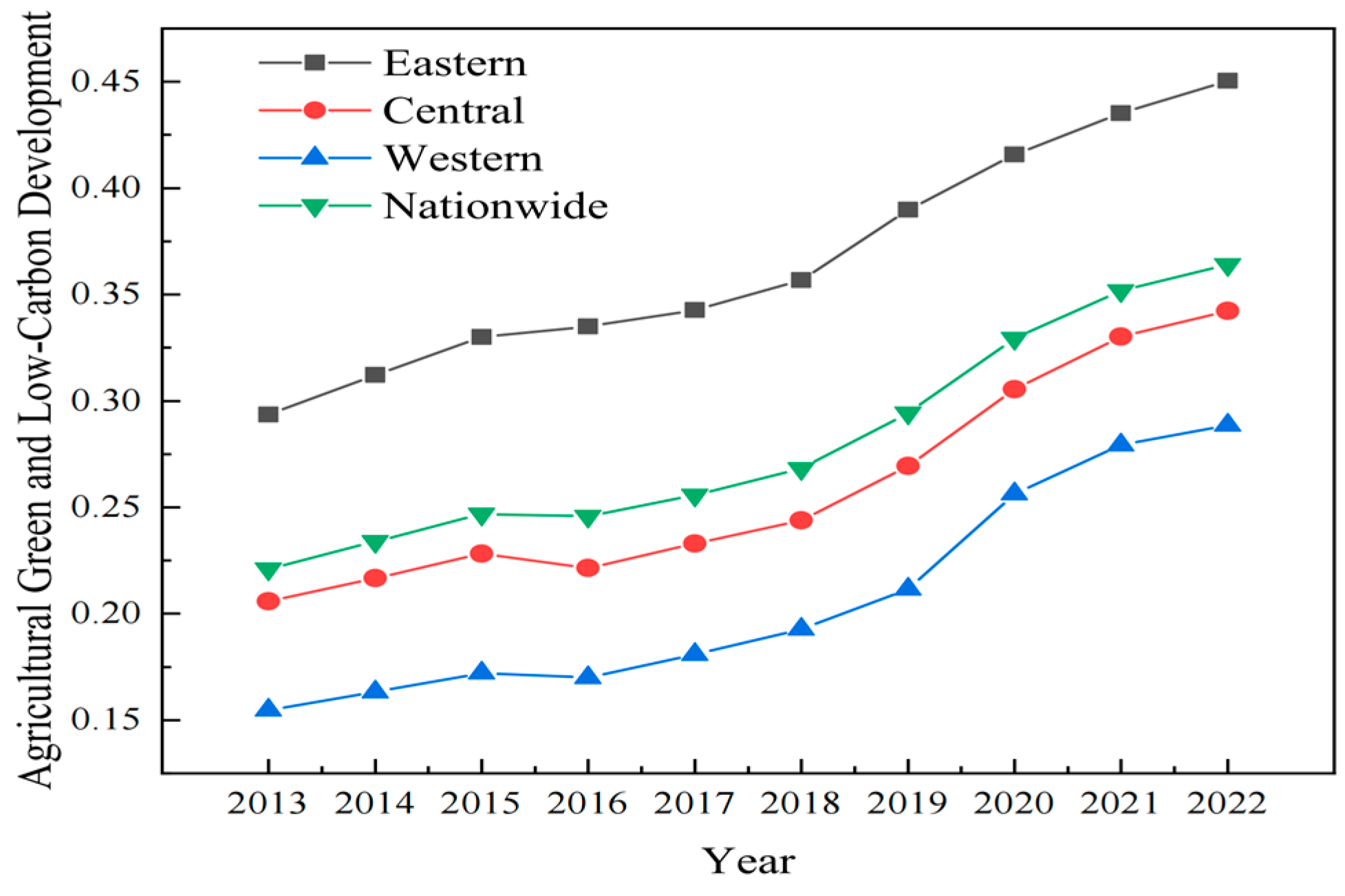
This study established a comprehensive evaluation system for LGA, adopted the TOPSIS entropy weight method to determine the index weights, and conducted a quantitative comparative analysis of the LGA levels in China from 2013 to 2022. Figure 2 reveals the differentiated temporal evolution patterns and regional characteristics of the LGA evaluation results. In addition, the overall evaluation results of LGA (Figure 3) and its spatial distribution characteristics (2013, 2016, 2019, 2022) were visualized through ArcGIS 10.8.2 software to analyze the spatial distribution pattern of LGA.
Table 2 presents the regional assessment results. During the sample period, provincial LGA scores ranged from 0.1070 to 0.6153, reflecting significant developmental differences. The indicators in most provinces show a gradual upward trend, indicating that LGA in all regions is continuously improving. However, after ten years of development, more than half of the provinces are still below the national average of 0.3641. Fujian Province leads with a ten-year average LGA score of 0.4631, followed by Beijing (0.4447), Tianjin (0.4329), and Hainan (0.4115), all from the eastern region. On the contrary, the national average score of Yunnan in the southwestern border area was the lowest at 0.1551. The LGA scores of Gansu (0.1681), Guizhou (0.1822), and Chongqing (0.1876) were also very low. All of them are located in the western region, highlighting the obvious regional east–west disparity.
To visualize national LGA dynamics, the Origin 2021 software was used to illustrate the time trend (Figure 2). National LGA has generally increased over the past decade, although it slightly declined in most regions from 2015 to 2016, except for the eastern region, where LGA rose from 0.3300 to 0.3350. After 2018, the economy resumed significant growth, which might be attributed to strengthened policy support, accelerated adoption of green technologies and improved implementation efficiency. The west achieved the highest growth rate (49.82%). The average ranking of LGA during the sample period is eastern (0.3661) > nationwide (0.2811) > central (0.2596) > western (0.2069), while the growth rate ranking is the opposite: western (86.62%) > central (66.25%) > nationwide (64.75%) > eastern (53.44%). This indicates that the east has maintained its leading position through superior infrastructure, policy advantages, and resource allocation, while the central and western regions have narrowed the development gap by leveraging the Rural Revitalization Strategy and modern agricultural technologies. Overall, the growth in the eastern region has slowed down, the central region has developed steadily, and the western region has entered a stage of rapid expansion.
Figure 3 visually depicts the trends of provinces through ArcGIS 10.8.2. In 2013, China’s LGA baseline exceeded 0.1 nationwide, indicating that early on, China had already recognized the significance of low-carbon and environmental protection, made efforts, and achieved certain results. However, the scores of the central and western provinces were below 0.3, while those of some eastern coastal provinces exceeded this threshold, indicating regional imbalance. By 2016, most provinces had shown steady improvement (mainly 0.1–0.3), and LGA in eastern developed provinces such as Fujian and Beijing exceeded 0.4. In 2019, the significant increase kept the LGA of most provinces between 0.2 and 0.4. Although Shanxi, Yunnan, and Gansu, which come from the central and western regions, remained below 0.2, Fujian and Beijing, which come from the east, exceeded 0.5, highlighting the polarization. By 2022, most central and western provinces had reached 0.2 to 0.4, while eastern provinces generally exceeded 0.4. Hainan performed outstandingly, surpassing Fujian and Beijing and breaking past 0.6 for the first time. However, the central and western provinces of Jiangxi, Shanxi, Gansu and Yunnan were still below 0.3, and there were still regional disparities.
In conclusion, the government’s emphasis and the continuous implementation of rural policies have steadily increased LGA, promoting the deep integration of the green development concept and the modernization of low-carbon agriculture. This progress has reduced carbon emissions and enhanced economic benefits, laying a solid foundation for rural revitalization and high-quality development. However, regional imbalance still exists: the east maintains a clear advantage, while the west, despite having recently shown a strong growth momentum driven by precise policy implementation and technological efficiency, remains relatively underdeveloped due to economic and technological constraints. The central region has demonstrated a stable development momentum, leveraging the advantages of major agricultural provinces (such as Henan Province) and aligning with the national food security strategy to maintain their growth momentum. It is worth noting Hainan’s extraordinary rise—in 2019, its LGA was still lower than that of the developed eastern provinces Beijing and Fujian, but by 2022, it had become the only province with an LGA score above 0.6. This is attributed to its eminent industrial access restrictions, land use control, carbon energy management, and significant environmental investment.
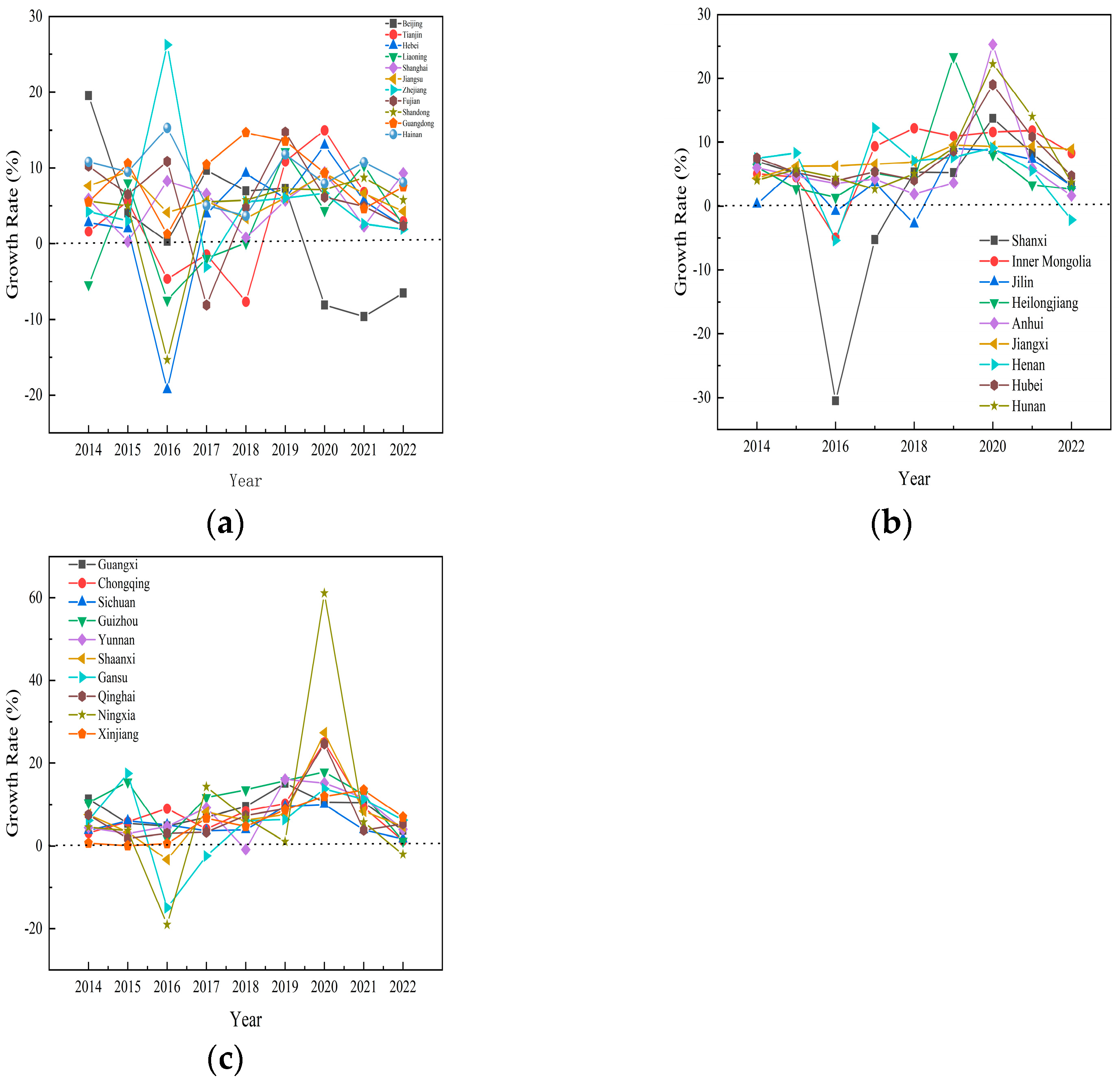
In terms of growth rate, the growth of each province fluctuated during the sample period, but ultimately the LGA growth rate of most provinces remained within the range of 0–10%, indicating that China’s LGA has entered a period of steady growth (Figure 4). In 2016, the growth rates in Shandong, Hebei, Shanxi, Ningxia, and Gansu dropped significantly, while in Zhejiang, the growth rate reached 26.23% during the same period. This is because both Shandong and Hebei are traditional major agricultural provinces and are facing the pain of transformation. Meanwhile, Zhejiang may have promoted the demonstration application of related environmental governance and green technologies by taking advantage of the G20 Summit held in Hangzhou. By 2020, the growth rate of LGA in all provinces generally rose. This was because 2020 was the final year of the national-level “National Agricultural Modernization Plan (2016–2020)” and the COVID-19 pandemic highlighted the importance of food security. All provinces attached greater importance to the necessity of developing agriculture. In 2022, the negative growth that Beijing, Ningxia, and Henan experienced might be due to Beijing gradually removing its non-capital function, while the results in Ningxia and Henan were because of their underdeveloped economies and the insufficient quality of universities within their provinces, making it difficult to retain relevant talents.
Drawing on Chen et al., this study uses natural breaks (Jenks) as the segmentation method to classify LGA into three major types: low, medium, and High [71]. Among them, [0, 0.2430] is defined as the low level, (0.2430, 0.3705] is defined as the medium level, and (0.3705, 0.6153] is defined as the high level (Table 3). Overall, after ten years of development, LGA in most provinces of China is at a medium to advanced level. Especially in 2021, when China achieved a moderately prosperous society in all respects, the number of provinces reaching a high level exceeded 10 for the first time, which also confirms that LGA in China has entered a period of steady development, as mentioned earlier.

4.2. Regional Disparities of LGA in China

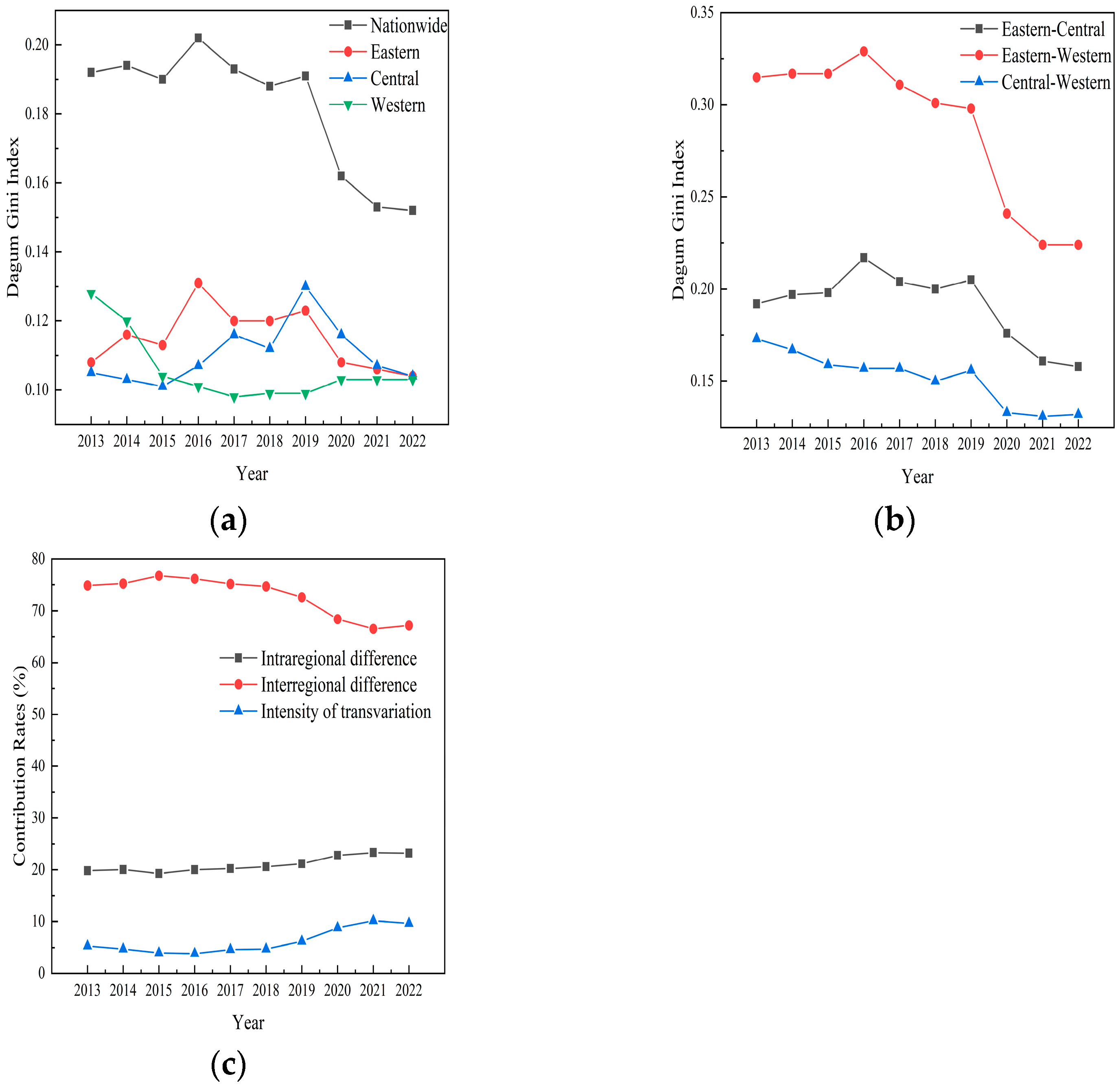
To gain a clearer understanding of the spatial development disparities of LGA in China, their temporal evolution, and the underlying sources of these disparities, this study categorizes China into three regions: eastern, central, and western. The Dagum Gini coefficient was used to measure intra-regional differences, inter-regional differences, and their respective contribution rates to the overall disparity in China’s LGA, with relevant results presented in Figure 5.

4.2.1. Inter-Region Disparities

What Figure 5a shows is the overall Dagum Gini coefficient dropped from 0.192 to 0.152 during the decade, indicating that policy support and investment in environmental technology have achieved remarkable results. However, notable fluctuations occurred, specifically in 2013, 2015, and 2018. These fluctuations can be attributed to major policy shifts: In 2013, the Chinese government formally introduced the concept of “The family farm”, promoting land transfer for intensive management, encouraging urban capital investment in rural areas, and increasing agricultural investment to construct high-standard farmland. These initiatives were initially adopted more readily by more developed regions, widening the gap with less developed areas. A similar internal driver was observed in 2015 with the strong national push for agricultural e-commerce. The 2018 policy emphasis on supply-side structural reform also contributed to the fluctuation. The substantial decline in 2019–2020 may be partially attributed to reduced economic activity during the COVID-19 pandemic narrowing disparities. Furthermore, the average Dagum Gini coefficient values across the decade ranked the regions as follows, indicating a higher degree of imbalance in the eastern region: eastern (0.1149) > central (0.1101) > western (0.1058). Overall, while intra-regional disparities fluctuated over the decade within each of the three regions, they remained relatively stable overall. Comparatively, the west showed a larger decline, dropping from 0.128 in 2013 to 0.1058 in 2022. Ultimately, intra-regional differences converged and stabilized around 0.11 across all regions. In summary, China’s LGA regional disparities significantly narrowed from 2013 to 2022, demonstrating the positive impact of policies and measures in coordinating regional development. However, achieving more balanced development requires continued focus on supporting lower-performing regions and strengthening inter-regional coordination and cooperation.

4.2.2. Inter-Regional Differences

Regarding inter-regional disparities (Figure 5b), differences between all three regional pairs decreased substantially. The reductions between eastern and central and central and western were similar in magnitude. The disparity between eastern and western reached its peak in 2016 (coefficient: 0.329) and exhibited the largest overall decrease over the decade (28.89%). Benefiting from optimized resource allocation, policy support, and economic assistance, the west significantly improved its LGA level in recent years. Its disparity with the central region stabilized around 0.132 in the last three years of the sample period. However, the gap with the eastern region remained pronounced, with the Dagum Gini coefficient still at 0.224 in 2022, highlighting the persistence of LGA imbalance as a major challenge requiring long-term efforts. In terms of trends, the central–western disparity declined steadily, with only a minor rebound in 2018. In contrast, both eastern–central and eastern–western disparities exhibited an “inverted M-shaped” pattern. This suggests that the western region, bolstered by national policy support, is catching up to the central region, narrowing their gap. As for the eastern region, it has fully utilized its advantages in education, technology and finance and has significantly outpaced the central and western regions in LGA. This trend also reflects the greater similarity in economic structure between the central and western regions.

4.2.3. Sources and Contributions of Disparities

Inter-regional disparity remains the primary contributor to China’s overall LGA inequality (Figure 5c). Although its contribution rate decreased from 74.86% to 67.14%, indicating the positive effect of policy adjustments and optimized resource allocation in reducing regional LGA gaps, it remains the dominant factor. This also implies that disparities at lower administrative levels (e.g., cities, counties) within regions are relatively less significant.

4.3. Analyzing Results from Spatial Autocorrelation Tests

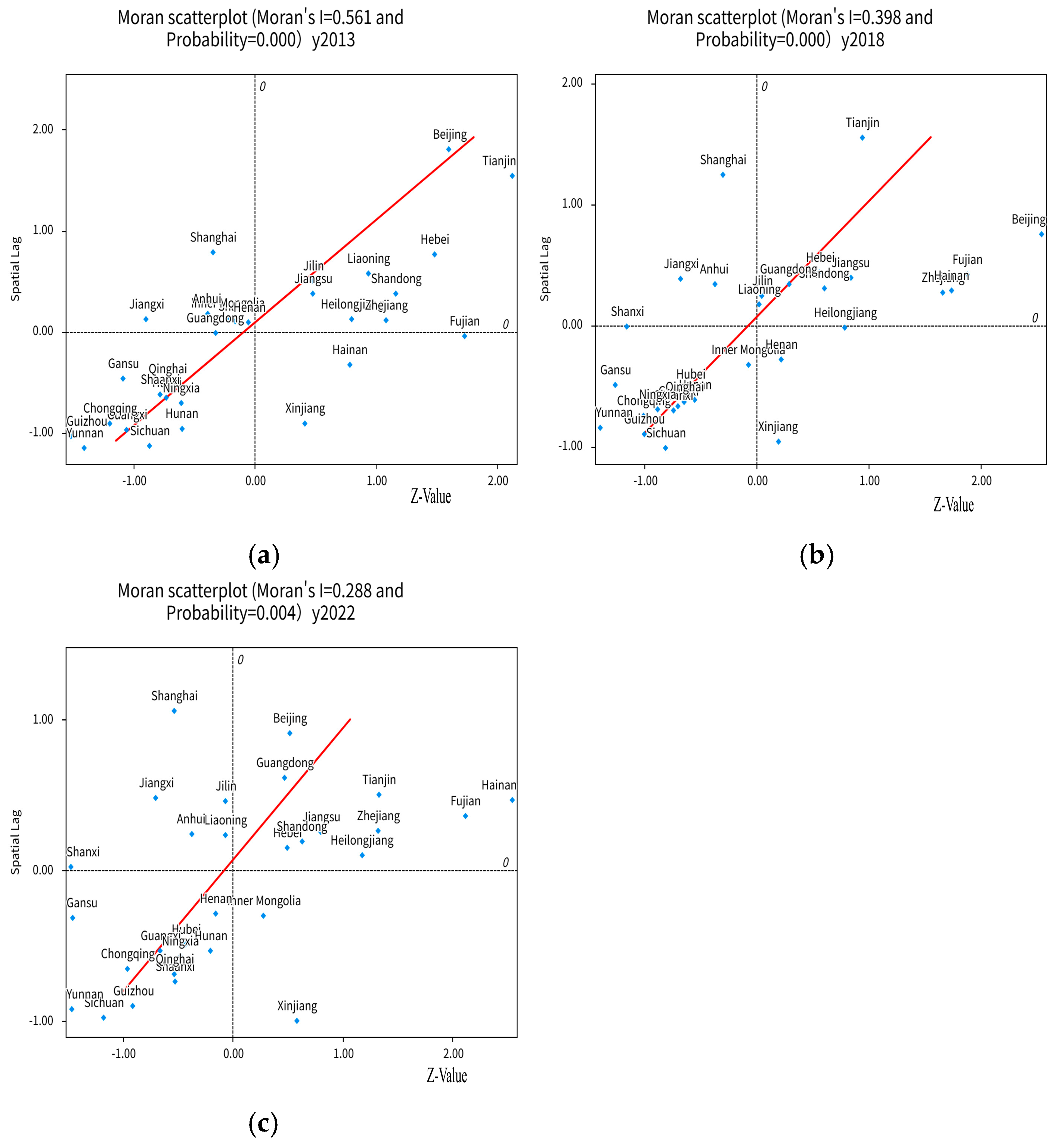
Under tremendous environmental pressure, the strategies adopted by local governments to deal with external shocks have shifted from high-end competition to imitation and reference. This transformation, through a demonstration effect, has pushed the LGA of developed provinces to catch up with the level of neighboring provinces; that is to say, it has promoted the improvement of the overall development level. The first law of geography states that spatial proximity strengthens the connection between subjects. LGA consists of three core elements: technology, optimized management, and efficient resource utilization. Innovative cooperation and geographical connections between adjacent provinces have further promoted the dissemination of technical knowledge, exerting a positive impact on LGA. Therefore, to verify the spatial correlation of LGA, this study evaluated the spatial agglomeration state of LGA through global Moran’s I and the 0–1 spatial weight matrix. To conduct a more in-depth analysis of its spatial distribution pattern, the study selected three key nodes, namely 2013, 2018, and 2022 (with a five-year interval), to carry out an in-depth analysis of the local spatial pattern. Figure 6 shows the relevant local Moran radiation diagram.
Based on Table 4, China’s LGA Moran’s Index remained consistently positive and statistically significant across the decade. This not only confirms the positive impact of geographical linkages on LGA but also lays the foundation for subsequent spatial dynamic evolution analysis. Notably, global Moran’s Index exhibited a continuous downward trend, with a particularly pronounced decline in 2015—dropping from 0.539 to 0.411, a reduction of 23.75%. This indicates that while spatial positive correlation persists, its influence on LGA is gradually weakening. Overall, LGA in China demonstrates significant spatial clustering: provinces with advanced LGA tend to be surrounded by similarly developed provinces, while less developed provinces are clustered with other underperforming regions. The weakening spatial autocorrelation over time may suggest increasing heterogeneity in the spatial distribution of key factors or variables.
Figure 6 displays the spatial distribution of LGA, covering three key time points (2013, 2018, and 2022). Most provinces are classified into the first and third groups, representing the positive-value group (developed provinces surrounded by developed neighboring provinces) and the negative-value group (underdeveloped provinces adjacent to underdeveloped regions), respectively. Further analysis shows that high-value agglomeration areas are mainly concentrated in eastern provinces such as Beijing, Tianjin, Hebei, Jiangsu, Zhejiang, and Guangdong. In contrast, western provinces like Gansu, Yunnan, and Guizhou primarily exhibit low–low clustering. Provinces in the second quadrant (low–high outliers) include Anhui, Shanghai, and Jiangxi, each with distinct underlying causes. Jiangxi—surrounded by economically advanced provinces like Fujian and Guangdong—experiences policy implementation lags (e.g., urban capital supporting rural areas, rural tourism development) due to funding shortages and limited urban population. Despite Shanghai’s economic strength, its scarcity of arable land compared to Jiangsu and Zhejiang constrains LGA development. Anhui’s status stems from both its lower economic development relative to Jiangsu/Zhejiang and adjacency to agricultural provinces like Henan and Shandong. The absence of low–high clusters in the west relates to the remote geography and harsh natural conditions. Notably, Xinjiang in the fourth quadrant (high–low outlier) stands apart from its neighbors due to its vast territory and thriving tourism industry, despite its remote northwestern location. Collectively, these findings underscore the strong spatial interdependence of China’s LGA and highlight the critical importance of spatial attributes in advancing LGA development.

4.4. Dynamic Changes in LGA

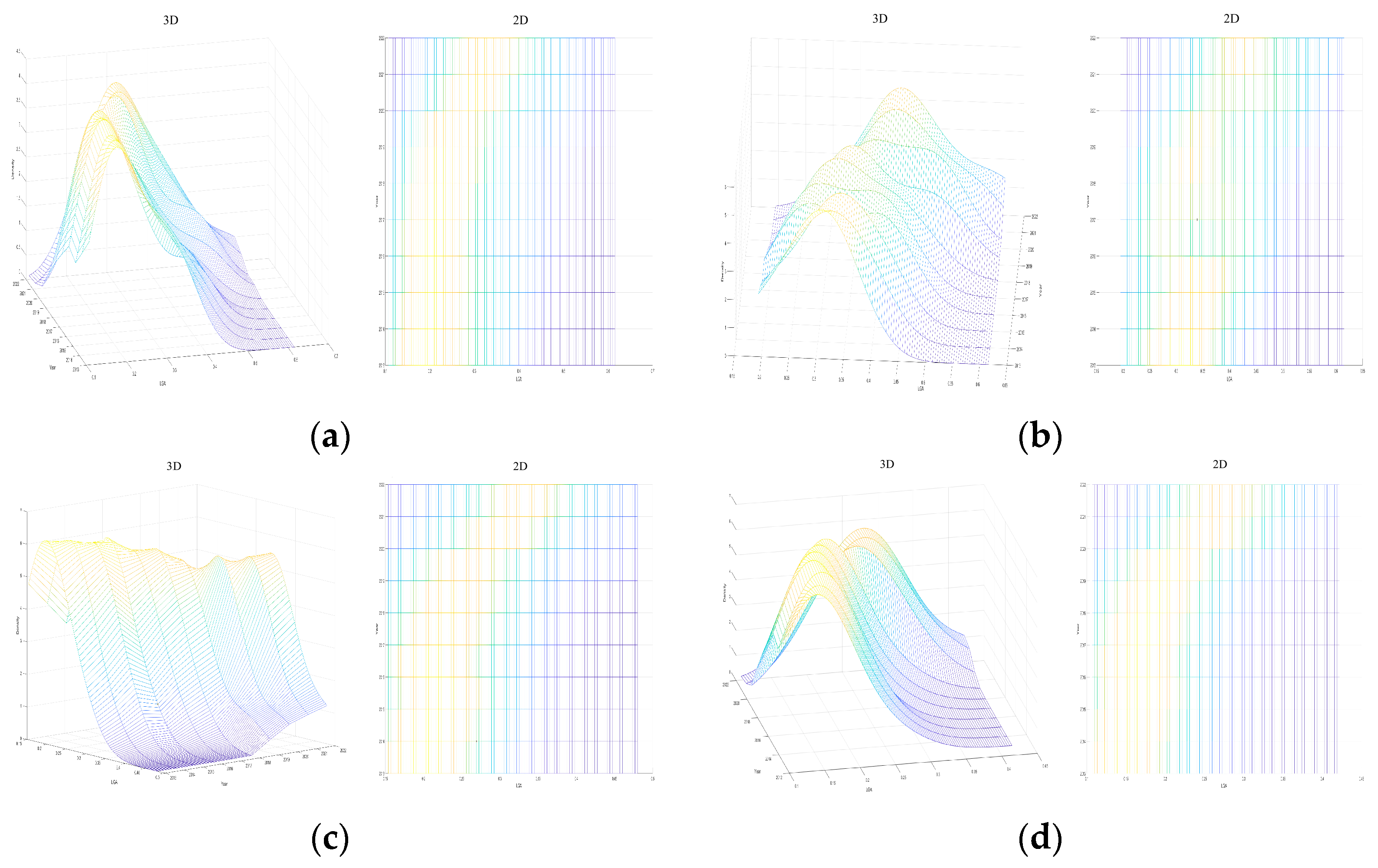
During this study period, we explored the dynamic evolution of national LGA through Kernel density estimation analysis (Figure 7). Figure 7a reveals that the Kernel density curve of the national LGA distribution from 2013 to 2022 has shifted to the right, which is consistent with the previous result of the annual increase in the national LGA. The initial evolution of the density curve in the eastern region presented the characteristics of “single peak–double peak–single peak”, indicating that there was a two-level differentiation phenomenon in China’s LGA during the sample period, but this phenomenon disappeared in 2022. The peak range has expanded and a “right tail” has emerged, indicating that the LGA levels in provinces such as Hainan and Fujian are relatively high.
The density curve in the eastern region generally shows a right-shifting trend (Figure 7b). The evolution trend of the curve in this area is “single peak–double peak–single peak”, indicating that there was once a two-level difference phenomenon in the eastern region. Subsequently, this phenomenon disappeared, and the internal differences tended to fuse, resulting in a right-tail phenomenon. The overall LGA is on the rise, but some provinces in Hainan, Fujian, and other places still maintain a relatively high LGA level.
In the central region (Figure 7c), the curve generally shifts to the right, with the peak height first decreasing and then rising again after 2019. In addition, since 2019, the “right tail” phenomenon has become increasingly prominent year by year, indicating that LGA in the central region increased year by year during the sample period. In 2019, due to the impact of the novel coronavirus pneumonia, the demand for grain increased, and LGA in Henan, Hubei, and other places was affected. Inner Mongolia and Heilongjiang, as major agricultural provinces, are located in the central region, but they are far from Hubei Province. This has widened the gap between them and other regions, leading to polarization. On the contrary, the growth rate in central regions such as Henan is relatively slow, resulting in the coexistence of convergence and polarization of internal differences, which is consistent with the calculation results of the Dagum Gini coefficient.
Finally, the curve in the western region has shifted to the right as a whole (Figure 7d), and there is a “right shift” phenomenon. This indicates that it is possible for it to transform into an efficient domain. In conclusion, LGA in China is on the rise, and there is polarization in various regions. Reasonable resource allocation and policy support are the keys to breaking the current predicament.

4.4.1. The Future Development Trend of LGA

Due to the limitations of KDE in predicting future development and changes—specifically its inability to quantify transition models or forecast future evolution—this study adopts the interquartile method to categorize China’s LGA into four levels from low to high: Type I (low, below 25%), Type II (medium-low, 25–50%), Type III (medium-high, 50–75%), and Type IV (high, above 75%). It examines the dynamic changes in China’s LGA over 1-to-4-year lag periods and predicts future trends.
In the Markov probability matrix (shown in Table 5), diagonal elements represent the probability that a region’s LGA level remains unchanged after T years, reflecting the stability of LGA in that region; non-diagonal elements indicate the likelihood of LGA shifting between different levels. With a one-year lag, diagonal probabilities stand at 80.00% (Type I), 74.29% (Type II), 74.24% (Type III), and 98.31% (Type IV), showing strong stability. A “club convergence effect” is evident: all regions have a higher probability of moving up than declining, and even low-level regions have a chance to rise to the medium-high level.
With a two-year lag, diagonal probabilities remain relatively high, but positive transition probabilities at the medium-low and medium-high levels increase significantly to 46.88% and 47.37% respectively—far exceeding their reverse transition probabilities. Meanwhile, low-level regions have a 62.67% probability of remaining unchanged, higher than their positive transition probability, indicating that breakthrough growth is more challenging for them compared to other regions.
The three-year lag scenario is similar to the two-year one, with a key difference: positive transition probabilities at the medium-low and medium-high levels surpass their stability probabilities, and medium-low regions even have the potential to leap two levels.
With a four-year lag, all regions except high-level ones have higher positive transition probabilities than stability probabilities, though all regions face a risk of reverse transition.
From the above, we can draw the following conclusions:
  • Currently, LGA in all Chinese regions is in a stable growth period with steady increases, though the growth rate has slowed—suggesting that China’s LGA has reached a certain developmental stage, consistent with previous findings.
  • Plagued by economic underdevelopment and harsh natural conditions, low-level regions face greater obstacles in moving up. However, once they overcome bottlenecks, they may achieve upgrades far beyond their current level.
  • Long-term accumulation can significantly boost the positive transition probabilities of all regions, which may stem from policy effectiveness lags.
  • High-level regions face an increasing risk of downgrading over time, and all regions are at risk of reverse transition. Thus, LGA development plans must be implemented steadily with long-term improvement measures.

4.4.2. The Results of Spatial Markov Chain Analysis

Given the strong spatial correlation revealed by the previous LGA spatial autocorrelation analysis, and the fact that the Traditional Markov Chain merely captures the transition probability of LGA while neglecting spatial correlation—thereby restricting its capacity to fully reflect regional dynamics—a spatial lag condition was incorporated into the traditional Markov transition probability matrix to explore the probability transition of LGA across China. Specific results are presented in Table 6 below.
First, the four transition probability matrices under different spatial lag types all differ from one another. This indicates that when neighboring provinces exhibit differences in LGA, the likelihood of the local province’s LGA being affected and undergoing a transition varies accordingly. Second, under different spatial lag types, the diagonal elements of the transition probability matrix are not strictly greater than the non-diagonal elements. This suggests that the probability of LGA “grade lock-in” has diminished under spatial spillover effects, a phenomenon that is particularly pronounced under Class III lag conditions. As for lag I, at both sides of the diagonal, for both low-level and high-level lag types, the values to the left of the diagonal are 0, meaning there is no negative impact on provinces at any level. Among these, except for medium-high-level provinces adjacent to low-level provinces and high-level provinces adjacent to high-level ones, the impact is positive. For medium-low-level and medium-high-level lag types, non-zero elements appear on both sides of the diagonal, indicating instability in provincial LGA when neighboring provinces are at medium-low or medium-high levels. While upward transitions can be achieved ideally, there is also a certain risk of downward transitions. Additionally, only transitions between adjacent grades occur, except for low-level areas near the medium level, making cross-grade leaps difficult to accomplish. Furthermore, different lag types exert varying influences on the same level. For example, the probability of an are with low-level LGA transitioning to medium-low level under a medium-high-level lag type is 66.67%, significantly higher than the transition probability under a medium-low-level lag type. Finally, the same lag type affects different grades differently. Under medium-high-level lag conditions, the probabilities of low-level, medium-low-level, and medium-high-level LGA achieving a one-grade upward transition are 66.67%, 28.57%, and 28.13%, respectively, showing a sequential decreasing trend. This indicates that transition probabilities are influenced not only by lag types but also by the initial LGA level.
When combined with the calculation results of the Traditional Markov Chain, it is evident that most provinces in China currently struggle to achieve upward leaps in the short term, with maintaining the status quo being more likely. Even if an upward leap is achieved, the risk of a downward transition must be guarded against. This stems from the inability of the current economic and industrial structure to adapt to the existing LGA development model. An exception is low-level provinces adjacent to medium-high-level provinces. Due to the significant grade gap between them and the low investment costs in low-level provinces—coupled with the fact that the industrial structure and scale of medium-high-level provinces are insufficient to generate a strong siphon effect—low-level provinces have, on the one hand, fully absorbed green agricultural technologies from medium-high-level provinces by leveraging the demonstration–imitation mechanism and geographical proximity. This has created a gradient potential for factor flow, driving human capital transfer and green capital injection, and indirectly fostering regional integrated governance such as joint environmental protection prevention and control and ecological compensation mechanisms in terms of policy allocation. In contrast, medium-low-level provinces lack the advantage of low investment costs and thus cannot attract higher-quality populations or green capital. Even when adjacent to high-level provinces, they may see their green production factors absorbed due to the siphon effect of high-level provinces.

4.5. Influencing Factors of LGA

To better explain in depth how LGA is affected, this study uses the Tobit regression model to analyze and explain the driving factors of LGA. Based on relevant research results [7,72,73,74,75,76], this study uses LGA to represent the level of low-carbon and green development in agriculture as the dependent variable, defined by the TOPSIS entropy weight method. Before conducting the regression analysis, this paper introduces the Variance Inflation Factor (VIF) to verify the model’s multicollinearity, thereby enhancing the stability of the model. The results show that the average value of the VIF is 3.29 (Table S7), and the VIF values of all influencing factors are less than 10, with no multicollinearity [77]. Eco represents the level of economic development and is defined by per capita GDP. Urb represents the level of urbanization and is defined by the urbanization rate. Als stands for agricultural large scale, defined by the ratio of sown area to the number of agricultural practitioners. Idu stands for the scale of the agricultural industry, which is defined by the ratio of the gross agricultural product to the area of cultivated land. Tec stands for expenditure on technology investment, which is defined by the ratio of research and development (R&D) funds to the total GDP. Ind represents the level of industrialization and is defined by the ratio of the added value of the secondary industry to the total GDP. Except for LGA as the dependent variable, all other indicators mentioned above are explanatory variables. α represents the undetermined coefficient and ε represents the random error term.
D i t = α 0 + α 1 ln E c o i t + α 2 U r b i t + α 3 A l s i t + α 4 I d u i t + α 5 T e c i t + α 6 I n d i t + ε i t
To fully understand the data characteristics of the main influencing factors during the research period, it is necessary to conduct descriptive statistical analysis on the relevant data to provide important reference basis for the subsequent regression model. The specific variables and data are shown in Table 7.
Based on the analysis results above, it is evident that there are significant regional disparities in China’s LGA in terms of spatial distribution. These disparities are likely closely linked to factors such as regional economic development levels, agricultural structures, resource endowments, and policy implementation effects. To more accurately identify the factors influencing LGA across different regions, this study conducted Tobit regression model analyses for the entire country, as well as the eastern, central, and western regions separately.
According to the regression results, the LR statistic for the national sample in China is 525.56 with a p-value less than 0.001, strongly rejecting the null hypothesis (i.e., no significant relationship between variables). For the eastern region, the LR statistic is 167.47 and the p-value is also less than 0.001, leading to the rejection of the null hypothesis. In the central region, the LR statistic stands at 75.41 with a p-value less than 0.001, similarly rejecting the null hypothesis. Finally, in the western region, the LR statistic is 148.45 and the p-value is less than 0.001, further confirming the significant influence of variables within the region. Therefore, this paper adopts a Tobit model with random effects to perform regression analyses on relevant variables, with specific results shown in Table 8. It is evident that China’s LGA progress is jointly influenced by multiple factors, including economic development level, urbanization progress, the scale of large-scale agriculture, agricultural industry scale, science and technology investment, and industrialization level. Regression results indicate that these factors exert varying degrees of influence across different regions and levels, indirectly reflecting the complex impact of regional disparities on LGA (Table 8).
It is evident that China’s LGA progress is jointly shaped by multiple factors, including economic development level, urbanization process, scale of large-scale agriculture, agricultural industry scale, science and technology investment, and industrialization degree. Regression analysis results reveal that these factors exert varying degrees of influence across different regions and levels, indirectly reflecting the complex impact of regional disparities on LGA (as shown in Table 8).
Firstly, during the study period, the economic development level has an influence coefficient of 0.0066 on national LGA, significant at the 1% level. Its impact coefficients on the eastern, central, and western regions are 0.0080 (1% significance), 0.0097 (10% significance), and 0.0121 (1% significance), respectively. This is because economic development not only drives capital input and infrastructure construction but also facilitates the application of more green technologies and sustainable agricultural models. Moreover, as economic levels improve, agricultural production gradually shifts toward energy conservation and environmental protection, thereby advancing agricultural green and low-carbon transformation.
Secondly, urbanization shows an impact coefficient of 0.2795 on national LGA during the study period, significant at the 1% level. Its regional coefficients are 0.2809 (eastern, 10% significance), −0.0508 (central, non-significant), and 0.2592 (western, 1% significance). The western region, with relatively low urbanization, can strengthen infrastructure through urbanization, promoting agricultural modernization and the adoption of green technologies. In the central region, where infrastructure is already relatively complete, further urbanization may squeeze the space for low-carbon agriculture, requiring additional policy support and financial investment. In the eastern region, with near-saturated urban populations and high urban–rural integration, suburban and modern green agriculture have taken shape, driving rural non-agricultural development and bringing more funds to rural areas. Thus, urbanization has optimized resource allocation and boosted LGA.
Thirdly, agricultural scale has an impact coefficient of 0.1067 on national LGA during the study period, significant at the 1% level. The corresponding coefficients for the eastern, central, and western regions are 0.0175 (non-significant), 0.1326 (1% significance), and 0.1635 (1% significance). In the central and western regions, the relatively low level of agricultural scale has resulted in higher production costs, while the scale of the agricultural industry’s operations has promoted farmer cooperation, formed green and low-carbon production models, and accelerated regional agricultural green development. In the eastern region, however, large-scale agriculture is already commonplace, so further expansion yields little benefit.
Furthermore, the scale of agricultural industry has an influence coefficient of 0.0115 on China’s LGA during the study period, significant at the 1% level. Its regional coefficients are 0.0124 (eastern, 1% significance), 0.0043 (central, non-significant), and 0.0078 (western, 1% significance). In the western region, which has a relatively low overall development level in terms of the scale of the agricultural industry, agricultural industries are more likely to foster local leading enterprises that drive LGA. In the central region, where a considerable number of leading enterprises already exist, transforming small-scale agricultural industries into large-scale agricultural industry does not directly benefit LGA, and further expanding the industrial scale has limited direct effects. The eastern region, with more resources and technical support, can leverage agricultural industry scale expansion to create economies of scale, facilitating green and low-carbon transformation and LGA improvement.
Also, science and technology expenditure show an impact coefficient of −0.2465 on China’s overall LGA during the study period (non-significant). Its regional coefficients are −0.6789 (eastern, non-significant), 5.1214 (central, 1% significance), and −3.7339 (western, 1% significance). The western region, still in an industry-driven economic stage, mainly supplies science and technology for “high pollution–high output” industries, with weak awareness of low-carbon and green development, leading to resource misallocation. In the central region, high industrialization has caused severe environmental degradation from high-carbon-emission industries, increasing the cost of the original production model. This has triggered a surge in environmental awareness and demand for low-carbon production, shifting science and technology supply toward “low pollution–high output” and prompting traditional agriculture to adopt green production technologies for low-carbon and green transformation. In the eastern region, where technology application is widespread and infrastructure is relatively complete, excessive technology investment may lead to inefficient resource allocation and even hinder agricultural green and low-carbon transformation, affecting overall development. Therefore, science and technology expenditure allocation should be precisely adjusted based on regional characteristics to maximize its promotional effect.
Finally, the industrialization process has an influence coefficient of 0.1311 on China’s LGA during the study period, significant at the 1% level. Its regional coefficients are −0.0633 (eastern, non-significant), 0.1151 (central, non-significant), and 0.1690 (western, 1% significance). In the western region, high-carbon-emission industries are a major source of total carbon emissions, highlighting the low carbon emissions of agriculture. In the central region, although environmental protection concepts are deeply rooted and all industries are undergoing green transformation, the lingering impact of high industrial carbon emissions results in a positive but non-significant effect. In the eastern region, industrialization is nearly saturated, and the service industry has gradually become the mainstay of the economy. With deindustrialization for service industry development as the main theme, promoting industrialization at this stage would not only occupy agricultural space but also increase rural carbon emissions.

5. Discussions, Conclusions, Suggestions, and Limitations

5.1. Discussions

From 2013 to 2022, the development of China’s LGA has experienced significant ups and downs, but overall, it has made progress and has now entered a period of steady growth. Heterogeneity analysis revealed that LGA was the highest in the eastern region and the lowest in the western region. The level in the eastern region was significantly higher than that in the central and western regions, which is similar to the research results of Cheng et al. [78], while the difference is that this study captured significant fluctuations of LGA in the starting and ending years of the “National Agricultural Modernization Plan (2016–2020)”, which indirectly reflects the effectiveness of this policy. Southeastern provinces such as Jiangsu, Zhejiang, and Fujian have made great progress and show a trend of gradually replacing the traditional major agricultural provinces in the north such as Beijing, Tianjin, Hebei, and Shandong. This is similar to the research results of Zhou & Wen [37], but the difference is that this article captures the progress of LGA in Hainan, which is a typical example of China’s deindustrialization, while emphasizing that Xinjiang, a western province, maintains its high LGA value due to its developed animal husbandry and tourism. In terms of differences, the coefficient of difference across the country dropped from 0.192 to 0.152. The coefficient of difference between the eastern, central, and western regions changed little. The difference was the greatest between the eastern and western regions, and the smallest between the western and central regions. However, since 2019, the coefficient of difference among various regions has gradually decreased. The main contribution to the source of differences in China’s LGA is the inter-regional differences. During the sample period, the overall level rose, but there was a “right trailing” phenomenon, indicating the existence of polarization. China’s LGA has significant spatial correlation, and most provinces are located in the first and third quadrants. Among them, the developed eastern regions such as Jiangsu and Zhejiang belong to the positive-value group, while the backward western provinces such as Gansu mainly belong to the negative-value group. This is similar to the research results of Zhou & Wen [39]. However, in terms of the sources of differences, this study holds that intra-group differences are the second largest source of differences, with a contribution rate of approximately 21.05%, acknowledging the LGA differences brought about by the formation of different standards and policy supplies in cities of different levels within the region (such as regional big cities, provincial capitals, etc.). In the short term, there will be a “club synergy” effect in the future. However, although it is difficult for low-level regions to break through, they have huge potential for upgrading, while high-level regions face the risk of downgrading. This is consistent with the calculation results of Yan et al. [38]. Meanwhile, Yan et al. believe that being adjacent to low-level provinces increases the difficulty of ascending, and vice versa is easier. On the contrary, this study holds that the stability is the poorest when adjacent to medium-low and medium-high level provinces. Of course, this also depends on the initial state of the province, which reflects the siphon effect of medium-high-level provinces on low-carbon and green production resources.
Through the analysis of the influencing factors, it is found that economic development significantly promotes LGA in all regions, indicating that economic growth provides crucial support for agricultural green and low-carbon transformation, which is consistent with Li et al. [53]; Urbanization benefits LGA in underdeveloped and highly developed regions but is less applicable to more developed regions undergoing industrial transformation which is similar to Hao & Liu [23]. Meanwhile, agricultural large scale can promote LGA in most regions but have little impact on highly developed areas. The agricultural industry scale promotes LGA in all regions except the central region, benefiting both underdeveloped and highly developed regions but not more developed regions undergoing industrial transformation. This result is almost the same as the research of Hu et al. [79]. Technology spending promotes LGA in more developed regions undergoing industrial structure transformation; inappropriate technology investment may lead to inefficient resource allocation. Cheng et al. also believed that technological progress does not always promote LGA [78]. Industrialization has a certain promotional effect on regions in the “high cost–high output” production mode but suppresses LGA after transformation, which is similar to that argued by Hao & Liu [23]. In conclusion, the results of this study align with the Environmental Kuznets Curve (EKC) [80]. Despite improvements in recent years, China is still in a “high cost–high output” production mode. Science and technology supply is gradually shifting toward low-carbon orientation, and high-pollution industries will soon be phased out, laying the groundwork for green industrial structure transformation.

5.2. Conclusions

Based on the theoretical framework of green and low-carbon agricultural development, this paper constructs an evaluation system covering agricultural greening, low-carbonization, modernization, and high efficiency. It measures the development levels of 30 Chinese provinces from 2013 to 2022 using the TOPSIS entropy method, analyzes their spatiotemporal characteristics with tools such as ArcGIS, Dagum Gini coefficient, Kernel density estimation, and Markov chain, and finally identifies the main influencing factors by combining with the Tobit regression model. The specific research contents are as follows.
China’s LGA shows significant regional differences and an unbalanced pattern. There is a marked gap in development levels among provinces: Hainan and Fujian, benefiting from effective policy implementation, technology promotion, and resource optimization, have LGA significantly higher than the national average. In contrast, regions with weak infrastructure, such as Gansu and Yunnan, lag in their transformation process and urgently need more policy support and resource input to accelerate development. Driven by both policies and technologies, China’s overall LGA has shown an annual growth trend. However, due to differences in resource endowments and policy implementation effects, the growth rates of various provinces are inconsistent.
Although LGA has generally increased across provinces, its spatial distribution is highly uneven, with prominent inter-provincial disparities—particularly between the eastern and western regions. Regional differences are the main source of such disparities, making narrowing regional gaps a key priority for the future. Dynamic development analysis shows that while LGA continues to rise nationwide and across regions, the peak height decreases and the width expands, reflecting the expansion of absolute differences and polarization. In terms of spatial correlation, LGA exhibits a strong spatial correlation: most provinces are surrounded by neighboring areas with similar development levels, and only few significant differences from their surroundings due to unique economic, policy, or natural conditions.
Future trend predictions indicate that LGA is currently in a period of slow growth, and most regions are expected to stabilize in the short term. In the long run, most regions have the potential to leap to higher levels—if low-level and medium-low-level regions can break through bottlenecks, they are expected to achieve cross-level leaps. Although high-level regions are likely to maintain their status quo, the risk of downgrading increases over time, and they should be wary of being surpassed. Moreover, regions at all development levels face the possibility of downgrading. The study also found that neighborhood characteristics have a significant impact: provinces adjacent to low-level or high-level areas face no downgrading risk; provinces adjacent to medium-low or medium-high level areas are at risk of downgrading; and those adjacent to medium-high-level areas cannot achieve cross-level leaps. Meanwhile, the spatial spillover effect and the province’s own LGA level jointly determine its evolutionary trajectory.
The key factors affecting China’s LGA include economic development, urbanization, agricultural large scale, agricultural industry scale, and industrialization. Economic development significantly promotes LGA in all regions, providing basic support for green transformation. Urbanization has a positive impact on regions other than the central region, but it also reflects the contradiction between industrial transformation and urban expansion. Large-scale agriculture has achieved significant results in regions other than the eastern region, improving efficiency and promoting the application of green technologies; however, in the eastern region, where large-scale agricultural industry operations are already widespread and the economy is service-oriented, continuing to promote the scale of the agricultural industry, operations has limited significance. The agricultural industry scale drives LGA in regions other than the central region, facilitating resource integration and sustainable development; in areas where leading enterprises have already formed at scale, the focus should be on encouraging more farmers to participate rather than simply expanding the scale. Technology expenditure is beneficial to regions other than the eastern region but shows a suppressive effect in the eastern region, highlighting regional differences in its effectiveness. Industrialization has a significant impact on LGA nationwide and in the western region but has little impact on the central and eastern regions, indicating that industry plays an economic driving role in the early stages of industrialization, while people pay more attention to environmental issues as industrialization advances.
In summary, promoting China’s LGA development requires coordinating multiple factors and flexibly adjusting policies and resource allocation based on regional differences. In the future, efforts should focus on strengthening technical support and policy funding to lay a solid foundation for agricultural green and low-carbon transformation.

5.3. Suggestions

First of all, a differentiated development strategy should be formulated to optimize resource allocation. At the national level, it is essential to roll out economic development policies with an environmental protection orientation, encourage the establishment of high-quality, organic, and eco-friendly agricultural leading enterprises in various regions, boost economic growth, advance urbanization, and drive the development of suburban agriculture and agricultural non-agriculturalization. Farmers should be encouraged to join agricultural cooperatives to expand and accelerate agricultural scaling. For the eastern regions, efforts should focus on reducing industrial emissions, phasing out outdated agricultural equipment and related agrochemicals, promoting the development of green agricultural technologies, and implementing the Internet of Things, drones, new energy agricultural tools, and intelligent dynamic agricultural detection systems. Rural science and technology service stations should be set up to facilitate the promotion of key technologies and the expansion of agricultural production scale. Additionally, leading agricultural enterprises should be supported to expand into other industries, achieve the integration of the primary, secondary, and tertiary industries, and complete urban–rural integration. For the central region, priority should be given to developing rural tourism and urban–rural service industries, gradually shifting the economic focus to the tertiary industry, fostering low-pollution primary and secondary industries, and promoting the scaling and integration of agricultural production. For the western regions, developing the economy and accelerating urbanization are crucial. They can leverage local resources such as tourism, energy, and mineral resources to develop characteristic industries based on local conditions, establish feedback policies to support agricultural development, and offer more preferential subsidy policies to attract talents and financial capital, thereby contributing to rural revitalization.
Secondly, inter-regional cooperation should be strengthened to achieve resource sharing. All regions need to enhance collaboration to share technologies and resources, build an integrated information exchange platform, enable leading enterprises in the central region to radiate their influence to the western region, and allow the western region to attract consumption from the central region through its high-quality tourism resources. This will facilitate multidirectional interactions of information flow, technology flow, and capital flow. Personalized green technology guidance and integrated agricultural solutions should be provided to farmers in green and low-carbon technologies such as soil improvement, organic substitution, and water–fertilizer integration, creating a fast track for the transformation of scientific research achievements into agricultural applications.
Finally, a region-wide coordinated policy system for green agriculture should be established to remove barriers to regional development. Government should, based on the development gradients and resource endowments of each district, establish a comprehensive institutional framework for agricultural low-carbon transformation covering the entire region, and eliminate regional disparities and technological gaps through unified policy benchmarks. Specific implementation paths include the following: In terms of policy incentives, a special guiding fund for green production should be set up, with gradient subsidies implemented for intelligent irrigation systems, substitution of biological agricultural supplies, organic farming models, and waste recycling projects. A dual mechanism of income tax reduction and equipment purchase subsidies should be promoted to drive the concentration of production factors in low-carbon projects. A transformation acceleration fund should be established for counties with weak technological capabilities to target breakthroughs in ecological transformation bottlenecks. In terms of technology penetration, a “three-in-one” technology diffusion network (digital service platform + science and technology commissioner system + professional farmer training) should be built, and a precise technology sinking project should be implemented. Technology adaptation transfer should be achieved through “field classrooms” and “expert village stays”, and a technology adoption tracking and evaluation mechanism should be established to increase the penetration and retention rates of low-carbon agronomy. Through the dual tracks of institutional guarantees and capacity building, a comprehensive and coordinated agricultural green transformation ecosystem should be formed, laying the governance foundation for a fair development pattern of low-carbon agriculture.
In a word, policy-makers should adopt differentiated strategies. In the high-level eastern regions, policies should focus on technological deepening and carbon market mechanisms (such as agricultural carbon sink trading), while in the low-level western regions, efforts should be made to enhance infrastructure construction and provide subsidies for green production technologies. Precise intervention: Given that regional differences are the main source, the central government should establish a cross-regional ecological compensation fund to encourage high-level regions to provide technical and financial assistance to low-income regions. Monitoring and assessment: It is suggested that the core indicators of LGA be incorporated into the performance appraisal system for local officials to encourage their long-term commitment. For farmers, although adopting low-carbon agricultural technologies increases investment in the short term, in the medium and long term, it can enhance the net income of the farm by improving soil quality, reducing the purchasing power of chemical fertilizers and the potential carbon sink benefits. Strengthening the role of cooperatives to establish a green agricultural product certification and traceability system enables farmers practicing low-carbon agriculture to sell their products at higher prices, creating a positive market incentive. In addition, the development of rural tourism also has the potential to drive the growth of LGA and increase revenue.

5.4. Limitations and Prospects

The primary deficiencies of the study: 1. It only analyzes the macro results and fails to conduct an analysis from a micro perspective (such as farmers’ behavior and cooperative relations); 2. Only the spatial correlation was proved, but no deeper research on LGA was conducted from the perspective of spatial metrology. 3. Only the external macro-environmental factors were analyzed, without conducting targeted research on influencing factors (such as the intensity of agricultural environmental support or science and technology investment, etc.). Later research can conduct in-depth analysis from a microscopic perspective in combination with more appropriate indicators in the future. 4. Although the TOPSIS entropy weight adopted in the study is objective, its weighting is completely dependent on the degree of data dispersion and may not fully reflect the absolute importance of certain indicators in theory. Future research can conduct robustness tests by combining subjective weighting methods such as the AHP (Analytic Hierarchy Process). In terms of data, the research is based on provincial panel data and cannot reveal the distribution differences within the province. Subsequent research can adopt data from municipal and county levels for more specific exploration. In addition, this article mainly reveals the correlation rather than the strict causal relationship. Although we attempted to control some variables, there might be a bias of omitted variables. Future research can adopt quasi-experimental methods (such as difference-in-differences) to more accurately identify policy effects. 5. In terms of the selection of system indicators, other related studies have paid more attention to the living standards of rural residents and the quality of life of farmers, such as Engel’s coefficient and forest coverage area. However, this study has limitations in this regard, mainly focusing on agricultural production itself and the carbon emissions it generates. 6. While this study provides a comprehensive analysis of LGA in China, it is crucial to acknowledge the contextual boundaries of our findings. The Chinese political and social system, characterized by a strong state capacity for policy implementation, a specific land tenure system, and a unique digital governance model, provides a distinct institutional environment for LGA. These specific characteristics are fundamental to the mechanisms observed in our study and may limit the direct extrapolation of our conclusions to other countries with markedly different socio-political frameworks. In the future, LGA from other backgrounds can be analyzed.

Supplementary Materials

The following supporting information can be downloaded at: https://www.mdpi.com/article/10.3390/agriculture15171853/s1, Table S1. The calculation results of the Spearman rank correlation coefficient among respective indicators; Table S2. The Spearman coefficients of the calculation results and rankings before and after removal; Table S3. Indicator Framework for Assessing China’s Low-carbon Green Agriculture Development Level (LGA) after removing B23, B41; Table S4. Indicator Framework for Assessing China’s Low-carbon Green Agriculture Development Level (LGA) after removing B23, B33; Table S5. Indicator Framework for Assessing China’s Low-carbon Green Agriculture Development Level (LGA) after removing B22, B41; Table S6. Indicator Framework for Assessing China’s Low-carbon Green Agriculture Development Level (LGA) after removing B22, B33; Table S7. Results of multicollinearity test.

Author Contributions

Writing—original draft, Z.M.; writing—review and editing, J.W. and P.Z.; data curation, Y.H. All authors have read and agreed to the published version of the manuscript.

Funding

General Report on the Preliminary Research of the 15th Five-Year Plan for Agricultural and Rural Development in Guangxi (Grant NO: GXZC2024-C3-O05884-JZZB); Research on Rural Construction and Governance and the Construction of Target index System for Rural Development during the 15th Five-Year Plan Period (Grant NO: GXZC2024-C3-005884-JZZB).

Institutional Review Board Statement

Not applicable.

Data Availability Statement

The raw data supporting the conclusions of this article will be made available by the authors on request.

Acknowledgments

The authors are grateful to the editors and the anonymous referees for their constructive and thorough comments, which contributed to the improvement of this study.

Conflicts of Interest

The authors declare no conflicts of interest.

References

  1. Wu, H.; Yang, Y.; Shen, Y. Agricultural Carbon Emissions in China: Estimation, Influencing Factors, and Projection of Peak Emissions. Pol. J. Environ. Stud. 2024, 33, 4791–4806. [Google Scholar] [CrossRef] [PubMed]
  2. Zhan, L.; Huang, X.; Xu, Z.; Huang, Z. Assessing the Coordination Development Level of Agricultural Economy and Ecology in China: Regional Disparities, Dynamics, and Barriers. Agriculture 2025, 15, 176. [Google Scholar] [CrossRef]
  3. Drinkwater, L.E.; Snapp, S.S. Nutrients in Agroecosystems: Rethinking the Management Paradigm. Adv. Agron. 2007, 92, 163–186. [Google Scholar]
  4. Norse, D. Low carbon agriculture: Objectives and policy pathways. Environ. Dev. 2012, 1, 25–39. [Google Scholar] [CrossRef]
  5. Liu, C.; Zheng, H. How social capital affects willingness of farmers to accept low-carbon agricultural technology (LAT)? A case study of Jiangsu, China. Int. J. Clim. Chang. Strateg. Manag. 2021, 13, 286–301. [Google Scholar] [CrossRef]
  6. Hou, J.; Hou, B. Farmers’ Adoption of Low-Carbon Agriculture in China: An Extended Theory of the Planned Behavior Model. Sustainability 2019, 11, 1399. [Google Scholar] [CrossRef]
  7. Cai, J.; Zheng, P.; Xie, Y.; Du, Z.; Li, X. Research on the impact of climate change on green and low-carbon development in agriculture. Ecol. Indic. 2025, 170, 113090. [Google Scholar] [CrossRef]
  8. Li, W.; Zeng, Y.; Zhang, Y.; Yi, K. The Coupling Coordination Relationship between Green Low-Carbon Agriculture and Socio-Economic Systems: Based on the Empirical Analysis of 31 Provinces in China. Pol. J. Environ. Stud. 2025, 34, 1641–1652. [Google Scholar] [CrossRef]
  9. Lu, Y.; Norse, D.; Powlson, D. Agriculture Green Development in China and the UK: Common objectives and converging policy pathways. Front. Agric. Sci. Eng. 2020, 7, 98–105. [Google Scholar] [CrossRef]
  10. Alotaibi, B.M. Riyadh Extension Agents’ Perceptions Regarding Organic Agriculture and Implications for Training. Ph.D. Thesis, The Pennsylvania State University, University Park, PA, USA, 26 March 2018. [Google Scholar]
  11. Paper, E.W.; Paper, E.W. Our Energy Future—Creating a Low Carbon Economy; White Paper; UK Department of Trade and Industry: London, UK, 2003. [Google Scholar]
  12. Luo, J.; Huang, M.; Bai, Y. Promoting green development of agriculture based on low-carbon policies and green preferences: An evolutionary game analysis. Environ. Dev. Sustain. 2024, 26, 6443–6470. [Google Scholar] [CrossRef]
  13. Liu, Y.; Deng, Y.; Peng, B. The Impact of Digital Financial Inclusion on Green and Low-Carbon Agricultural Development. Agriculture 2023, 13, 1748. [Google Scholar] [CrossRef]
  14. Liang, Y.; Pan, T.; Cai, Y.; Yu, J.; Choun, L. The impact of green and low carbon agricultural production on farmers’ income in minority areas: A case study of Y Town, Zhijin County, Guizhou Province. Front. Sustain. Food Syst. 2024, 8, 1358471. [Google Scholar] [CrossRef]
  15. Ran, G.; Wang, G.; Du, H.; Lv, M. Relationship of Cooperative Management and Green and Low-Carbon Transition of Agriculture and Its Impacts: A Case Study of the Western Tarim River Basin. Sustainability 2023, 15, 8900. [Google Scholar] [CrossRef]
  16. Wang, W.; Guo, L.; Li, Y.; Su, M.; Lin, Y.; de Perthuis, C.; Ju, X.; Lin, E.; Moran, D. Greenhouse gas intensity of three main crops and implications for low-carbon agriculture in China. Clim. Change 2015, 128, 57–70. [Google Scholar] [CrossRef]
  17. Jiang, Q.; Li, J.; Si, H.; Su, Y. The Impact of the Digital Economy on Agricultural Green Development: Evidence from China. Agriculture 2022, 12, 1107. [Google Scholar] [CrossRef]
  18. Qi, Z.; You, Y. The Impact of the Rural Digital Economy on Agricultural Green Development and Its Mechanism: Empirical Evidence from China. Sustainability 2024, 16, 3594. [Google Scholar] [CrossRef]
  19. Dai, X.; Li, Y.; Qi, Y.; Chen, Y.; Yan, D.; Xia, K.; He, S.; He, Y. Coupling Agricultural Green Development and Park City Development: An Empirical Analysis from Chengdu, China. Agriculture 2025, 15, 248. [Google Scholar] [CrossRef]
  20. Mo, L.; Chen, S.; Wan, S.; Zhou, L.; Wang, S. How Can the Protection of Important Agricultural Heritage Sites Contribute to the Green Development of Agriculture: Evidence from China. Agriculture 2025, 15, 166. [Google Scholar] [CrossRef]
  21. Li, R.; Cui, W. Spatial–Temporal Evolution and Influencing Factors of Arable Land Green and Low-Carbon Utilization in the Yangtze River Delta from the Perspective of Carbon Neutrality. Sustainability 2024, 16, 6889. [Google Scholar] [CrossRef]
  22. Li, Z.; Zhao, D.; Yan, H. Evaluation and dynamic mechanism of green low-carbon transformation of agriculture in Yangtze River Delta region. Int. J. Low-Carbon Technol. 2024, 19, 2431–2445. [Google Scholar] [CrossRef]
  23. Hao, D.; Liu, W. Will structural adjustment and financial support affect low-carbon agricultural production in the Yellow River Basin? Environ. Sci. Pollut. Res. 2024, 31, 47330–47349. [Google Scholar] [CrossRef] [PubMed]
  24. He, P.; Zhang, J.; Li, W. The role of agricultural green production technologies in improving low-carbon efficiency in China: Necessary but not effective. J. Environ. Manag. 2021, 293, 112837. [Google Scholar] [CrossRef] [PubMed]
  25. Lu, H.; Chen, Y.; Luo, J. Development of green and low-carbon agriculture through grain production agglomeration and agricultural environmental efficiency improvement in China. J. Environ. Manag. 2024, 442, 141128. [Google Scholar] [CrossRef]
  26. Fred, A.O.; Anthony, M.K. Modeling assessment of groundwater vulnerability to contamination risk in a typical basement terrain using TOPSIS-entropy developed vulnerability data mining technique. Heliyon 2023, 9, e18371. [Google Scholar] [CrossRef]
  27. Li, J.; Zheng, Z.; Xu, Y.; Hang, S.; Gong, H. Optimization of coupling crop and livestock production system’s eco-efficiency in northern China based on a life cycle assessment and data envelopment analysis method. Sci. Total Environ. 2024, 921, 170852. [Google Scholar] [CrossRef]
  28. Chen, C.; Zhang, H. Evaluation of Green Development Level of Mianyang Agriculture, Based on the Entropy Weight Method. Sustainability 2023, 15, 7589. [Google Scholar] [CrossRef]
  29. Wang, L.; Li, N.; Xie, Q. Dynamic evolution and obstacle factor analysis of green development in China’s agriculture and rural areas based on entropy-based TOPSIS model. Heliyon 2024, 10, e27248. [Google Scholar] [CrossRef]
  30. Xingcun, F.; Yang, Y.; WeiChiao, H. The impact of green taxation on green low-carbon development in Yangtze River Delta region of China-based on mediating effect model and spatial Durbin model. Environ. Sci. Pollut. Res. 2023, 30, 103674–103689. [Google Scholar]
  31. Abadi, M.; Moore, D.R. Selection of Circular Proposals in Building Projects: An MCDM Model for Lifecycle Circularity Assessments Using AHP. Buildings 2022, 12, 1110. [Google Scholar] [CrossRef]
  32. Weijun, W.; Hongshan, Z. Evaluation of Low Carbon Economy Development in China’s Provinces: Based on Entropy-OWA Algorithm and Grey Correlation Improvement TOPSIS. IOP Conf. Ser. Earth Environ. Sci. 2019, 371, 032028. [Google Scholar]
  33. Ye, M.; Deng, F.; Yang, L.; Liang, X. Evaluation of regional low-carbon circular economy development: A case study in Sichuan province, China. Int. J. Clim. Chang. Strateg. Manag. 2022, 14, 54–77. [Google Scholar] [CrossRef]
  34. Zhou, J.; Xu, N.; Zhang, W.; Ning, X. Can agricultural low-carbon development benefit from urbanization?-Empirical evidence from China’s new-type urbanization pilot policy. J. Environ. Manag. 2024, 435, 140388. [Google Scholar] [CrossRef]
  35. Yanwei, Q.; Huailiang, L.; Jianbo, Z. Prediction model and demonstration of regional agricultural carbon emissions based on Isomap–ACO–ET: A case study of Guangdong Province, China. Sci. Rep. 2023, 13, 12688. [Google Scholar]
  36. Martindale, W.; Saeidan, A.; Javazm, F.; ÆHollands, T.; Duong, L.; Jagtap, S. Mapping the path to decarbonised agri-food products: A hybrid geographic information system and life cycle inventory methodology for assessing sustainable agriculture. Int. J. Food Sci. Technol. 2024, 59, 6078–6086. [Google Scholar] [CrossRef]
  37. Zhou, F.; Wen, C. Research on the Evolution of the Spatial Association Network Structure and Driving Factors of China’s Agricultural Green Development. Agriculture 2024, 14, 683. [Google Scholar] [CrossRef]
  38. Yan, J.; Tang, Z.; Guan, Y.; Xie, M.; Huang, Y. Analysis of Measurement, Regional Differences, Convergence and Dynamic Evolutionary Trends of the Green Production Level in Chinese Agriculture. Agriculture 2023, 13, 2016. [Google Scholar] [CrossRef]
  39. Zhou, F.; Wen, C. Research on the Level of Agricultural Green Development, Regional Disparities, and Dynamic Distribution Evolution in China from the Perspective of Sustainable Development. Agriculture 2023, 13, 1441. [Google Scholar] [CrossRef]
  40. Liu, F.; Wang, L.; Gao, J.; Liu, Y. Study on the Coupling Coordination Relationship Between Rural Tourism and Agricultural Green Development Level: A Case Study of Jiangxi Province. Agriculture 2025, 15, 874. [Google Scholar] [CrossRef]
  41. He, Y.; Fang, G.; Qi, C.; Gu, Y. Research on the Spatial Correlation Network and Driving Mechanism of Agricultural Green Development in China. Agriculture 2025, 15, 693. [Google Scholar] [CrossRef]
  42. Liu, J. How Does Agricultural Green Transformation Improve Residents’ Health? Empirical Evidence from China. Agriculture 2024, 14, 1085. [Google Scholar] [CrossRef]
  43. Chi, Y.; Liu, D.H.; Zhang, M.X. Island carrying capacity for three development types: Ecological resource, agricultural production, and urban construction. Heliyon 2022, 8, e12232. [Google Scholar] [CrossRef]
  44. Nong, W.; Wen, J.; He, J. Spatial-Temporal Variations and Driving Factors of the Coupling and Coordination Level of the Digital Economy and Sustainable Rural Development: A Case Study of China. Agriculture 2024, 14, 849. [Google Scholar] [CrossRef]
  45. National Bureau of Statistics of China. National Data Center. Available online: http://data.stats.gov.cn/ (accessed on 18 June 2025).
  46. National Bureau of Statistics of China. China Statistical Yearbook; China Statistics Press: Beijing, China, 2023.
  47. National Bureau of Statistics of China; Department of Population and Employment Statistics. China Population and Employment Statistical Yearbook; China Statistics Press: Beijing, China, 2023.
  48. National Bureau of Statistics of China; Department of Rural Socioeconomic Survey. China Rural Statistical Yearbook; China Statistics Press: Beijing, China, 2023.
  49. National Bureau of Statistics of China; Ministry of Science and Technology of China. China Statistical Yearbook on Science and Technology; China Statistics Press: Beijing, China, 2023.
  50. Wind Economic Database. Available online: https://www.wind.com.cn/portal/zh/EDB/index.html (accessed on 18 June 2025).
  51. de Moraes Sa, J.C.; Lal, R.; Cerri, C.C.; Lorenz, K.; Hungria, M.; de Faccio Carvalho, P.C. Low-carbon agriculture in South America to mitigate global climate change and advance food security. Environ. Int. 2017, 98, 102–112. [Google Scholar] [CrossRef] [PubMed]
  52. Li, Y.; Fan, Z.; Jiang, G.; Quan, Z. Addressing the Differences in Farmers’ Willingness and Behavior Regarding Developing Green Agriculture-A Case Study in Xichuan County, China. Land 2021, 10, 316. [Google Scholar] [CrossRef]
  53. Li, Z.; Jin, M.; Cheng, J. Economic growth of green agriculture and its influencing factors in china: Based on emergy theory and spatial econometric model. Environ. Dev. Sustain. 2021, 23, 15494–15512. [Google Scholar] [CrossRef]
  54. Wang, W.; Li, K.; Liu, Y.; Lian, J.; Hong, S. A system dynamics model analysis for policy impacts on green agriculture development: A case of the Sichuan Tibetan Area. J. Environ. Manag. 2022, 371, 133562. [Google Scholar] [CrossRef]
  55. Bai, Y.; Deng, X.; Jiang, S.; Zhao, Z.; Miao, Y. Relationship between climate change and low-carbon agricultural production: A case study in Hebei Province, China. Ecol. Indic. 2019, 105, 438–447. [Google Scholar] [CrossRef]
  56. Liu, D.; Zhu, X.; Wang, Y. China’s agricultural green total factor productivity based on carbon emission: An analysis of evolution trend and influencing factors. J. Environ. Manag. 2021, 278, 123692. [Google Scholar] [CrossRef]
  57. Zhaoyan, L.; Hongmei, L. Coordination Development of” Water-Energy-Food” System in China’s Agriculture and Its Influencing Factors. Econ. Geogr. 2024, 44, 177–186. [Google Scholar]
  58. Hu, C.; Fan, J.; Chen, J. Spatial and Temporal Characteristics and Drivers of Agricultural Carbon Emissions in Jiangsu Province, China. Int. J. Environ. Res. Public Health 2022, 19, 12463. [Google Scholar] [CrossRef]
  59. Zhang, Z.; Li, Y.; Elahi, E.; Wang, Y. Comprehensive Evaluation of Agricultural Modernization Levels. Sustainability 2022, 14, 5069. [Google Scholar] [CrossRef]
  60. Huang, K.; Tang, W.; Zhou, F. Agricultural Productive Services and Ecological Efficiency of Cultivated Land Use: Evidence from Hunan Province, China. Pol. J. Environ. Stud. 2024, 33, 5127–5140. [Google Scholar] [CrossRef]
  61. Wang, Y.; Zhou, Q. Evaluation of development of agricultural modernization in central China. IERI Procedia 2013, 4, 417–424. [Google Scholar] [CrossRef]
  62. Li, Y.; You, X.; Sun, X.; Chen, J. Dynamic assessment and pathway optimization of agricultural modernization in China under the sustainability framework: An empirical study based on dynamic QCA analysis. J. Environ. Manag. 2024, 479, 144072. [Google Scholar] [CrossRef]
  63. Peng, H.; Yang, F.; Yue, O. How Rural Industry Revitalization Affects Farmers’ Incomes in China. Sustainability 2024, 16, 9182. [Google Scholar] [CrossRef]
  64. Wang, J.; Zhao, Y.; Li, X.; Zhou, Y.; Zhao, K.; Wang, H.; Shakweer, W.M.E.S. Multimodal fusion-based detection method of estrus cows using multisource data inspired by hidden Markov model algorithms. Comput. Electron. Agric. 2025, 235, 110391. [Google Scholar] [CrossRef]
  65. Luo, L.; Nie, Q.; Jiang, Y.; Luo, F.; Wei, J.; Cui, Y. Spatiotemporal Dynamics and Spatial Spillover Effects of Resilience in China’s Agricultural Economy. Agriculture 2024, 14, 1522. [Google Scholar] [CrossRef]
  66. Zhu, Q.; Chen, J.; Rui, H.; Hamoud, Y.A.; Algarawi, A.M.; Okla, M.K.; Zhu, L.; Shaghaleh, H. Collaborative management measures of subsurface drainage and bio-organic fertilizer application for coastal sunflower (Helianthus annuus L.) based on TOPSIS entropy weight method. PLoS ONE 2025, 20, e0318571. [Google Scholar] [CrossRef]
  67. Zhao, X.; Wang, Z.; Xia, W.; Hu, B.; Vasa, L.; Nassani, A.A. Unlocking energy efficiency: Exploring the dynamic evolution and regional correlations in the Huaihe Eco-economic Belt. Gondwana Res. 2025, 145, 57–70. [Google Scholar] [CrossRef]
  68. Zhou, Y.; Lu, H.; Wan, X.; Wen, D.; Xie, X. KDE-DE: A kernel density estimation-based differential entropy method for EEG feature extraction in spatial cognitive evaluation. Biomed. Signal Process. Control 2025, 110, 108209. [Google Scholar] [CrossRef]
  69. Huu, T.; Lokuge, W.; Karunasena, W.; Setunge, S. Markov-based deterioration prediction and asset management of floodway structures. Sustain. Resil. Infrastruct. 2022, 7, 789–802. [Google Scholar]
  70. Liu, J.; Fang, Y.; Ma, Y.; Chi, Y. Digital economy, industrial agglomeration, and green innovation efficiency: Empirical analysis based on Chinese data. J. Appl. Econ. 2024, 27, 2289723. [Google Scholar] [CrossRef]
  71. Chen, J.; Yang, S.T.; Li, H.W.; Zhang, B.; Lv, J.R. Research on Geographical Environment Unit Division Based on the Method of Natural Breaks (Jenks). ISPRS—Int. Arch. Photogramm. Remote Sens. Spat. Inf. Sci. 2013, 40, 47–50. [Google Scholar] [CrossRef]
  72. Dong, D.; Wang, J. Air pollution as a substantial threat to the improvement of agricultural total factor productivity: Global evidence. Environ. Int. 2023, 173, 107842. [Google Scholar] [CrossRef]
  73. Song, Y.; Zhang, B.; Wang, J.; Kwek, K. The impact of climate change on China’s agricultural green total factor. Technol. Forecast. Soc. Chang. 2022, 185, 122054. [Google Scholar] [CrossRef]
  74. Gao, Y.; Zhang, M.; Wang, K.; Wen, F.; Liu, F. The Carbon Emissions Reduction Effect of Green Agricultural Subsidy Policy: A Quasi-Natural Experiment. Sustainability 2024, 16, 5210. [Google Scholar] [CrossRef]
  75. Lu, F.; Meng, J.; Cheng, B. How does improving agricultural mechanization affect the green development of agriculture? Evidence from China. J. Environ. Manag. 2024, 472, 143298. [Google Scholar] [CrossRef]
  76. Xu, J.; Zha, T. Chinese Urbanisation and Food Security. Oxid. Commun. 2016, 39, 2159–2170. [Google Scholar]
  77. Hu, J.; Zhang, X.; Wang, T. Spatial Spillover Effects of Resource Misallocation on the Green Total Factor Productivity in Chinese Agriculture. Int. J. Environ. Res. Public Health 2022, 19, 15718. [Google Scholar] [CrossRef]
  78. Cheng, L.; Gao, Y.; Dai, X. Spatio-temporal comprehensive measurement of China’s agricultural green development level and associated influencing factors. PLoS ONE 2023, 18, e0288599. [Google Scholar] [CrossRef] [PubMed]
  79. Hu, Y.; Li, B.; Zhang, Z.; Wang, J. Farm size and agricultural technology progress: Evidence from China. J. Rural Stud. 2022, 93, 417–429. [Google Scholar] [CrossRef]
  80. Dinda, S. Environmental Kuznets Curve Hypothesis: A Survey. Ecol. Econ. 2004, 49, 431–455. [Google Scholar] [CrossRef]
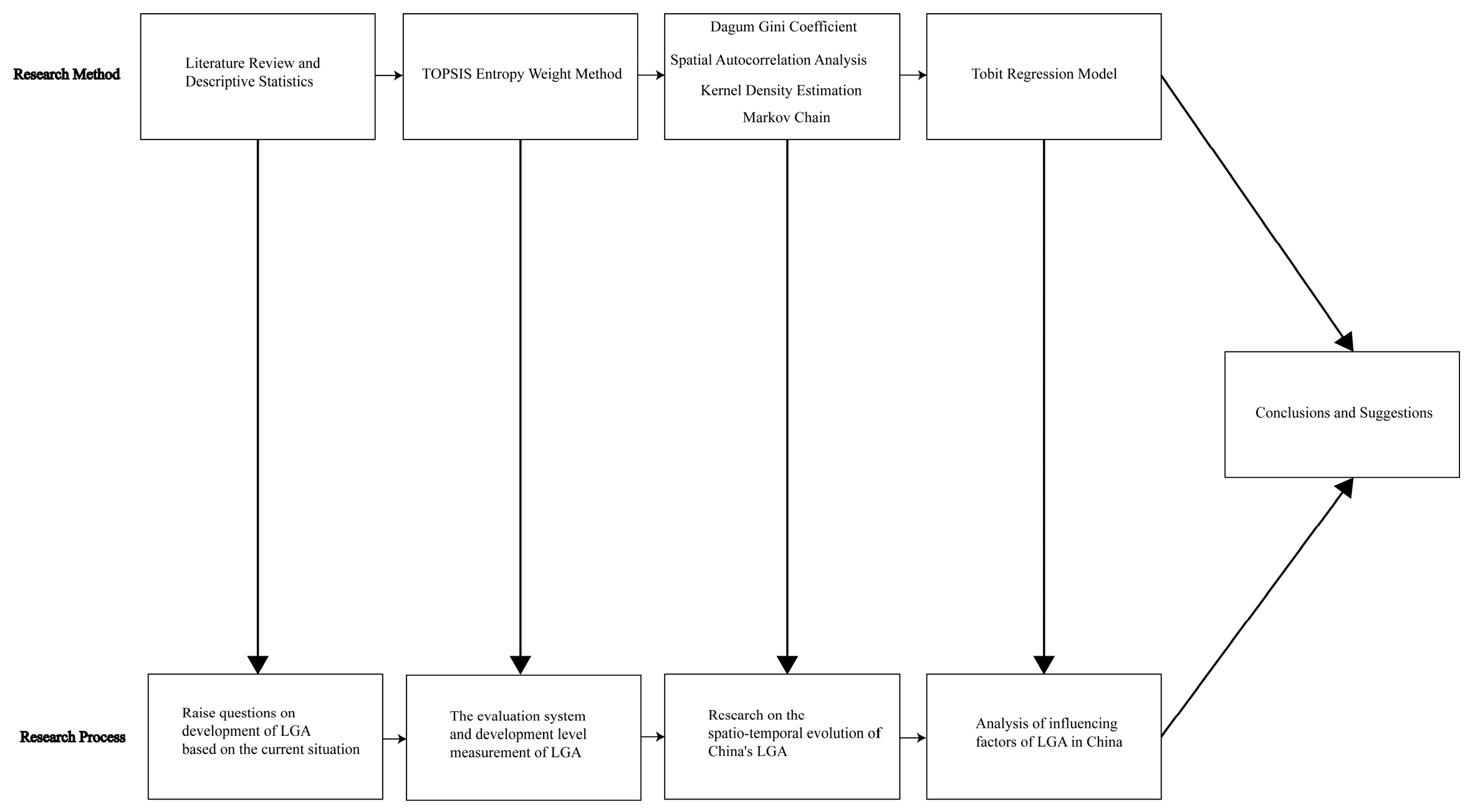
Figure 1. Technical route.
Agriculture 15 01853 g001
Figure 2. China’s regional LGA (2013–2022).
Agriculture 15 01853 g002
Figure 3. (a) LGA in China in 2013. (b) LGA in China in 2016. (c) LGA in China in 2019. (d) LGA in China in 2022.
Agriculture 15 01853 g003
Figure 4. (a) The growth rate of the eastern LGA. (b) The growth rate of the central LGA. (c) The growth rate of the western LGA.
Agriculture 15 01853 g004
Figure 5. (a) the intra-regional development differences in LGA in China from 2013 to 2022. (b) The inter-regional development differences in LGA in China from 2013 to 2022. (c) The main factors of the uneven LGA in China from 2013 to 2022.
Agriculture 15 01853 g005
Figure 6. (a) Local Moran scatter plots (2013). (b) Local Moran scatter plots (2018). (c) Local Moran scatter plots (2022).
Agriculture 15 01853 g006
Figure 7. (a) The 3D and 2D KDE of LGA in China (2013–2022). (b) The 3D and 2D KDE of LGA in the east (2013–2022). (c) The 3D and 2D KDE of LGA in the central region (2013–2022). (d) The 3D and 2D KDE of LGA in the west (2013–2022).
Agriculture 15 01853 g007
Table 1. Indicator framework for assessing China’s low-carbon green agriculture development level (LGA).
Main IndexFirst-Tier IndexesSecond-Tier IndexesExplanationNature of IndicatorsWeight
B11 Application intensity of agricultural chemical fertilizersFertilizer application rate/sown area [38]0.0287
B12 Intensity of pesticide applicationPesticide application rate/sown area [38]0.0110
A1 Agricultural greeningB13 Usage strength of agricultural plastic filmPlastic film usage/sown area [38]0.0148
B14 Diesel energy consumption intensityAgricultural diesel usage/cultivated area by machinery [57]0.0130
B21 Regional agricultural carbon emission scaleTotal agricultural carbon emissions/regional administrative area0.0131
LGA in ChinaA2 Low-carbonization of agricultureB22 Agricultural carbon emission densityTotal agricultural carbon emissions/sown area [58]0.0081
B23 Agricultural carbon emission intensityTotal agricultural carbon emissions/
gross agricultural product [37]
0.0172
A3 Agricultural modernizationB31 Level of agricultural mechanizationTotal power of agricultural machinery/
sown area [59]
+0.0881
B32 Irrigation efficiencyEffective irrigation/
sown area [39]
+0.0903
B33 Socialization of agricultural productionOutput value of agriculture, forestry, animal husbandry, and fishery services/sown area [60]+0.1727
B34 Total power of agricultural machinery per capitaTotal power of agricultural machinery/agricultural practitioners [61]+0.1253
A4 Agricultural efficiency improvementB41 Agricultural output levelAgricultural output value/sown area [38]+0.1197
B42 Grain production levelGrain output/sown area [38]+0.0846
B43 Agricultural labor efficiencyAgricultural output value/
agricultural workforce [37,59]
+0.0961
B44 Per capita total output value of agriculture, forestry, animal husbandry, and fisheryTotal output value of agriculture, forestry, animal husbandry, and fishery/rural practitioners [62,63]+0.1173
Table 2. The results of LGA in China.
Province/Year2013201420152016201720182019202020212022
Beijing0.34070.40720.42370.42490.46610.49850.53490.49160.44440.4154
Tianjin0.37940.38550.40710.38820.38270.35340.39180.45050.48120.4955
Hebei0.33180.34100.34780.28070.29170.31880.33780.38160.40320.4125
Shanxi0.20850.22310.23450.16300.15440.16260.17110.19460.21070.2174
Inner Mongolia0.20380.21410.22380.21280.23270.26110.28970.32330.36160.3916
Liaoning0.29060.27490.29710.27500.26970.26990.30270.31600.34870.3571
Jilin0.25650.25730.27230.27000.27990.27210.29670.32250.34610.3571
Heilongjiang0.28060.29770.30590.31010.32600.33950.41900.45280.46800.4802
Shanghai0.19480.20630.20680.22390.23860.24050.25420.27820.28460.3111
Jiangsu0.25680.27640.30270.31520.33290.34400.36490.39880.42520.4434
Zhejiang0.30180.31460.32410.40910.39660.41840.44360.47300.48540.4948
Anhui0.19150.20300.21250.22010.22940.23370.24220.30350.32140.3266
Fujian0.35000.38590.41090.45550.41860.43860.50320.53410.56040.5736
Jiangxi0.15380.16050.17050.18120.19310.20640.22610.24720.27030.2943
Shandong0.30800.32530.34160.28920.30510.32260.34590.37050.40290.4261
Henan0.21700.23330.25270.23910.26830.28740.30940.33760.35630.3486
Hubei0.16600.17850.18790.19530.20580.21420.23270.27690.30690.3214
Hunan0.17570.18280.19330.20190.20720.21770.23750.29040.33110.3434
Guangdong0.19640.20720.22910.23200.25620.29380.33350.36470.38160.4102
Guangxi0.14170.15780.16640.17440.18650.20430.23520.26010.28740.2982
Hainan0.27940.30960.33900.39090.41060.42570.47590.51380.56910.6153
Chongqing0.13120.13530.14320.15610.16250.17620.19430.24300.26560.2690
Sichuan0.15570.16150.17130.18000.18660.19390.21250.23380.24290.2470
Guizhou0.10700.11820.13650.13900.15530.17640.20420.24070.27060.2739
Yunnan0.11530.12040.12400.12980.14180.14060.16320.18800.20990.2183
Shaanxi0.16220.17450.18030.17430.18860.20040.21560.27460.29770.3117
Gansu0.13940.14800.17390.14790.14430.15310.16290.18540.20640.2193
Qinghai0.16710.17960.18290.18850.19480.20910.22790.28420.29500.3108
Ningxia0.17520.18310.18990.15370.17570.18760.18960.30550.32300.3164
Xinjiang0.25190.25370.25390.25540.27250.28540.31030.34750.39450.4219
Average0.22100.23390.24690.24590.25580.26820.29430.32950.35170.3641
Table 3. Classification of the number of provinces with LGA at different levels from 2013 to 2022.
Classes/Year2013201420152016201720182019202020212022
Low18181718161514543
Medium11910791110171515
High133554681112
Table 4. Global Moran’s I Index of LGA in China from 2013 to 2022.
YearIndexProbabilityValue of Z
20130.561 ***0.0004.856
20140.550 ***0.0004.766
20150.539 ***0.0004.674
20160.411 ***0.0003.632
20170.426 ***0.0003.758
20180.398 ***0.0003.529
20190.372 ***0.0003.316
20200.342 ***0.0013.073
20210.281 ***0.0052.571
20220.288 ***0.0042.629
Note: *** indicates significance at the 1% levels.
Table 5. Traditional Markov transition probability matrix for LGA in China from 2013 to 2022.
PeriodLag TypeIIIIIIIVObserved Value
T1I0.80000.18670.01330.000075
II0.01430.74290.24290.000070
III0.00000.03030.74240.227366
IV0.00000.00000.01690.983159
T2I0.62670.34670.02670.000075
II0.03120.50000.46880.000064
III0.00000.03510.49120.473757
IV0.00000.00000.02270.977344
T3I0.47220.44440.08330.000072
II0.05080.32200.55930.067859
III0.00000.04350.30430.652246
IV0.00000.00000.03030.969733
T4I0.34330.50750.14930.000067
II0.06120.16330.59180.183749
III0.00000.05130.23080.717939
IV0.00000.00000.04000.960025
Table 6. Spatial Markov transition probability matrix for LGA in China from 2013 to 2022.
Lag Typet/(t + 1)IIIIIIIVObserved Value
II0.87760.12240.00000.000049
II0.00000.85710.14290.00007
III0.00000.00001.00000.00002
IV0.00000.00000.00000.00000
III0.75000.20000.05000.000020
II0.02380.73810.23810.000042
III0.00000.03850.80770.153826
IV0.00000.00000.00001.00007
IIII0.33330.66670.00000.00006
II0.00000.71430.28570.000014
III0.00000.03130.68750.281332
IV0.00000.00000.04550.954522
IVI0.00000.00000.00000.00000
II0.00000.71430.28570.00007
III0.00000.00000.66670.33336
IV0.00000.00000.00001.000030
Table 7. The descriptive statistical analysis of variables.
VariableNMeanSDMinMax
LGA3000.28110.10270.10700.6153
Eco3006.19163.21480.600019.0000
Urb3000.61030.11380.38200.8960
Als3000.81060.41850.20902.9362
Idu3006.41204.22631.282124.9968
Tec3000.01840.01160.00450.0683
Ind3000.39630.07700.15870.5576
Table 8. The results of the Tobit model.
VariableNationwideEasternCentralWestern
Eco0.0066 ***
(0.0015)
0.0080 ***
(0.0024)
0.0097 *
(0.0050)
0.0121 ***
(0.0034)
Urb0.2795 ***
(0.0585)
0.2809 *
(0.1536)
−0.0508
(0.1810)
0.2592 ***
(0.0856)
Als0.1067 ***
(0.0093)
0.0175
(0.0274)
0.1326 ***
(0.0101)
0.1635 ***
(0.0148)
Idu0.0115 ***
(0.0008)
0.0124 ***
(0.0011)
0.0043
(0.0028)
0.0078 ***
(0.0013)
Tec−0.2465
(0.6004)
−0.6789
(0.9474)
5.1214 ***
(1.2240)
−3.7339 ***
(0.9585)
Ind0.1311 ***
(0.0505)
−0.0633
(0.1401)
0.1151
(0.0773)
0.1690 ***
(0.0582)
_cons−0.1377 ***
(0.0435)
0.0121
(0.1354)
−0.0505
(0.1055)
−0.1615 ***
(0.0508)
sigma_u0.0664 ***
(0.0088)
0.0866 ***
(0.0206)
0.0308 ***
(0.0077)
0.0365 ***
(0.0085)
sigma_e0.0211 ***
(0.0009)
0.0254 ***
(0.0018)
0.0167 ***
(0.0013)
0.0113 ***
(0.0008)
N30011090100
Note: * and *** indicate significance at the 10% and 1% levels, respectively.
Disclaimer/Publisher’s Note: The statements, opinions and data contained in all publications are solely those of the individual author(s) and contributor(s) and not of MDPI and/or the editor(s). MDPI and/or the editor(s) disclaim responsibility for any injury to people or property resulting from any ideas, methods, instructions or products referred to in the content.