High-Accuracy Cotton Field Mapping and Spatiotemporal Evolution Analysis of Continuous Cropping Using Multi-Source Remote Sensing Feature Fusion and Advanced Deep Learning

Abstract

Cotton is a globally strategic crop that plays a crucial role in sustaining national economies and livelihoods. To address the challenges of accurate cotton field extraction in the complex planting environments of Xinjiang’s Alaer reclamation area, a cotton field identification model was developed that integrates multi-source satellite remote sensing data with machine learning methods. Using imagery from Sentinel-2, GF-1, and Landsat 8, we performed feature fusion using principal component, Gram–Schmidt (GS), and neural network techniques. Analyses of spectral, vegetation, and texture features revealed that the GS-fused blue bands of Sentinel-2 and Landsat 8 exhibited optimal performance, with a mean value of 16,725, a standard deviation of 2290, and an information entropy of 8.55. These metrics improved by 10,529, 168, and 0.28, respectively, compared with the original Landsat 8 data. In comparative classification experiments, the endmember-based random forest classifier (RFC) achieved the best traditional classification performance, with a kappa value of 0.963 and an overall accuracy (OA) of 97.22% based on 250 samples, resulting in a cotton-field extraction error of 38.58 km². By enhancing the deep learning model, we proposed a U-Net architecture that incorporated a Convolutional Block Attention Module and Atrous Spatial Pyramid Pooling. Using the GS-fused blue band data, the model achieved significantly improved accuracy, with a kappa coefficient of 0.988 and an OA of 98.56%. This advancement reduced the area estimation error to 25.42 km², representing a 34.1% decrease compared with that of the RFC. Based on the optimal model, we constructed a digital map of continuous cotton cropping from 2021 to 2023, which revealed a consistent decline in cotton acreage within the reclaimed areas. This finding underscores the effectiveness of crop rotation policies in mitigating the adverse effects of large-scale monoculture practices. This study confirms that the synergistic integration of multi-source satellite feature fusion and deep learning significantly improves crop identification accuracy, providing reliable technical support for agricultural policy formulation and sustainable farmland management.

1. Introduction

Cotton, a globally significant strategic resource, plays a crucial role in sustaining national economies and livelihoods [1]. Currently, the cotton industry faces challenges, such as high labor and material costs, particularly in large-scale cotton field management and water resource allocation [2]. Traditional methods for gathering information about cotton fields rely on manual sampling surveys, which are inefficient, prone to errors and omissions, inadequate for meeting the demands of rapid and accurate data collection [3], and time-consuming. Annual data on cotton planting areas at the regional level primarily depend on remote sensing estimates and sampling surveys, which involve temporal delays and limit their applicability in production decision-making. Therefore, accurate and rapid monitoring of cotton-planting areas is essential to ensure robust, large-scale, and sustainable production [4,5].

The rapid advancement of satellite remote sensing technology has enabled innovative solutions for the precise extraction of regional crop information by providing high-frequency, multi-dimensional observational data [6]. This technology effectively covers extensive crop cultivation areas and provides timely and dynamic crop-planting information, thus facilitating the development of precise and smart agricultural systems. When combined with machine learning algorithms, the spectral characteristics of multispectral data can improve the accuracy of the model [7]. Maruf et al. [8] utilized the extensive spectral imagery provided by Sentinel-2 for land cover mapping, achieving an accuracy of 74% using the maximum likelihood classification (MLC) method. They also assessed flood damage across various land categories, resulting in an overall accuracy (OA) of 89.06%. Wu et al. [9] used gradient-boosting decision trees (GBDT) to develop a model correlating brightness temperature with associated surface parameters. Their findings indicated that the GBDT model achieved a correlation coefficient of 67.9% and demonstrated greater effectiveness during summer and in regions characterized by complex land cover. Guo et al. [10] applied partial least squares regression (PLSR) to estimate soil organic carbon using various spectral bands and the normalized difference vegetation index (NDVI) from multiple satellite imagery datasets. Their results demonstrated that machine learning techniques outperformed traditional regression models in terms of predictive capability.

Previous studies have shown that individual satellites equipped with multispectral sensors face challenges in simultaneously achieving extensive coverage and high-precision imagery [11]. Then, researchers have looked to fuse images from satellites equipped with various sensors to improve the accuracy of satellite-based monitoring. Zhang et al. [12] used Landsat and Sentinel-2 images combined with logistic regression models to evaluate the effectiveness of the Enhanced Vegetation Index (EVI), NDVI, and Land Surface Water Index (LSWI) in assessing the annual start of season (SOS). Zhou et al. [13] used images from Landsat-5, Landsat-7, Landsat-8, Sentinel-2, and Gaofen-1 satellites, demonstrating that the Plastic-Mulched Citrus Index (PMCI) performed exceptionally well in extracting plastic-mulched citrus (PMC) across various observation dates, with an OA exceeding 0.91 for both intra-annual and inter-annual PMC detection. Kang et al. [14] integrated spectral, Synthetic Aperture Radar (SAR), topographic, and textural features using the Google Earth Engine (GEE) platform. Their findings demonstrated that incorporating SAR data along with topographic and textural features improved both user and producer accuracies for tea plantation classification, increasing from 89.3% and 85.9% to 95.8% and 91.7%, respectively. Li et al. [15] used multi-temporal Landsat 8 Operational Land Imager (OLI) images, combined with spectral angle mapping and decision tree classification, to extract the major crop distributions in the Eastern Xinrong District of Datong City. They compared their results with those obtained using the MLC. However, research on cotton field area extraction using multi-source remote sensing data remains limited, with only a few studies successfully mapping cotton fields using high-resolution imagery. Zhang et al. [16] extracted cotton field maps in Northern Xinjiang using Sentinel-1/2 remote sensing data, combined with a random forest classifier (RFC) and multi-scale image segmentation, achieving an OA of 0.932 and a kappa coefficient of 0.813.

With the rapid advancement of deep learning, its applications in semantic segmentation and object detection in remote sensing imagery have become increasingly widespread [17,18,19,20]. Li et al. [21] conducted a comparative study using Gaofen-1 satellite imagery of Zhengzhou City to evaluate four different deep-learning network models for automated land cover classification in high-resolution images. Their results demonstrated that the MS-EfficientUNet method achieved optimal performance in classifying land cover in Zhengzhou with an OA of 0.7981. Cultivated land yielded the highest intersection over union (IoU) and F1-Score values of 0.7801 and 0.8764, respectively. Zhong et al. [22] developed two types of deep learning models, long short-term memory (LSTM) and 1D convolutional neural networks (NNs), for summer crop classification. Their study revealed that the Conv1D-based model achieved the highest accuracy of 85.54% and an F1-score of 0.73. Seydi et al. [23] proposed a novel framework that integrates deep convolutional neural networks (CNNs) with dual attention modules (DAM) using Sentinel-2 time-series datasets to generate accurate and timely crop-type maps. This approach achieved exceptional performance, with an OA of 98.54% and a kappa coefficient of 0.981.

In summary, although numerous studies have utilized multi-source satellite image fusion for land-cover area estimation, studies specifically focusing on cotton field extraction remain limited. Although multi-source remote sensing data fusion has demonstrated improved classification accuracy for certain crops, the effectiveness of modeling varies significantly depending on the fusion methodologies and feature band selection approaches used. Furthermore, the development of training datasets is constrained by regional geographical characteristics, climatic conditions, and spatiotemporal spectral variations in observational parameters, which collectively restrict the spatial transferability of the existing cotton field mapping techniques. The Alar Reclamation Zone in Xinjiang, China, with its extensive cotton cultivation area, offers a wealth of annotated data for cotton field extraction. This presents a critical opportunity to develop high-precision, cost-effective models for cotton field mapping and acreage estimation by integrating satellite remote sensing with deep-learning technologies. The development of such models is particularly urgent to address the current agricultural needs.

This study focused on cotton cultivation areas in Alar City, Xinjiang, using a comprehensive methodological framework to address the existing research gaps. Multi-temporal satellite imagery was collected from GF-1, Landsat 8, and Sentinel-2, implementing three distinct fusion approaches, principal component (PC), Gram–Schmidt (GS), and NN, to integrate spectral, vegetation, and texture features through pairwise image fusion. The optimal feature bands for cotton field extraction were systematically selected through quantitative evaluation using three key metrics: the mean value, standard deviation, and information entropy. A confusion matrix analysis was conducted to comparatively assess the performance of various machine-learning classifiers in cotton field extraction, using optimally fused imagery. Furthermore, the U-Net architecture was improved by incorporating both a Convolutional Block Attention Module (CBAM) and an Atrous Spatial Pyramid Pooling (ASPP) module to improve mapping accuracy. This study evaluated the estimates of cotton cultivation areas derived from various classifiers, using multi-dimensional assessment criteria. This study provides scientifically robust data support and decision-making support for multispectral remote sensing methodologies in cotton field extraction, particularly for addressing the challenges of precision agriculture in arid regions.

2. Materials and Methods

2.1. Overview of the Study Area

The Alar Reclamation Zone occupies a unique geographical position (80°30′ E–81°58′ E, 40°22′ N–40°57′ N), serving as an ecological transition area between the Taklimakan Desert and the southern foothills of the Tianshan Mountains, with a total area of 6923.4 km² [24], as shown in Figure 1. The soil exhibits a distinct northwest-to-southeast inclination bordered by the Aksu, Tailan, and Tarim Rivers. Arar City has a warm temperate extreme continental arid desert climate, with an extreme maximum temperature of 35 °C and an extreme minimum temperature of −28 °C. The average annual precipitation is 40.1–82.5 mm, and the average annual evaporation is 1876.6–2558.9 mm. In 2022, the agricultural output value reached 28.6 billion yuan, with cotton plantations covering 247,000 mu (approximately 164,667 hectares). After the implementation of crop rotation policies, cultivated areas decreased by 42,000 mu (approximately 28,000 hectares), resulting in 205,000 mu (approximately 136,667 hectares) of cotton fields in 2023 [25]. In addition to cotton, the Alar Reclamation Zone also cultivates other crops such as wheat and corn. According to regional agricultural statistics, in 2023, the planting area of corn was about 68,000 mu (45,333 hectares), while the planting area of wheat was about 53,000 mu (35,333 hectares). The phenological period of cotton in this area usually includes emergence (from late April to early May), budding (from late May to mid-June), flowering (from July to August), and bolling (from September) These stages are very consistent with the date of satellite image acquisition, ensuring the best spectral separability in the process of feature extraction.

2.2. Remote Sensing Data Acquisition

GF-1 satellite data were acquired from the U.S. Geological Survey’s (USGS) Earth Explorer platform. The GF-1 satellite is equipped with two primary sensors: a Panchromatic and Multispectral Sensor (PMS) and a Wide Field View (WFV) Sensor. The PMS includes two panchromatic multispectral imaging systems capable of capturing panchromatic images at 2 m resolution and multispectral images at 8 m resolution [26]. The WFV sensor integrates four multispectral cameras, delivering data at a 16 m resolution across four spectral bands: blue, green, red, and near-infrared (NIR). Sentinel-2A, operating at an altitude of 786 km, is a high-resolution multispectral imaging mission that provides comprehensive land-cover information, including data on vegetation, water bodies, and soil characteristics. The satellite has a swath width of 290 km and covers 13 spectral bands with ground sampling distances of 10, 20, and 60 m, featuring a 5-day revisit cycle [27,28]. For this study, 10 m resolution bands (blue, green, red, and NIR) were used, along with three red-edge bands from a Multispectral Instrument (MSI). Landsat 8 OLI data were used, specifically the 30 m resolution bands (blue, green, red, and NIR), with detailed spectral characteristics (

Table 1. Satellite image band parameters.

GF-1				Sentinel-2				Landsat 8
Name	Band	Resolution	Wavelength Range	Name	Band	Resolution	Wavelength Range	Name	Band	Resolution	Wavelength Range
Blue	Band2	16 m	150–520 nm	Blue	Band2	10 m	490–560 nm	Blue	Band2	30 m	450–515 nm
Green	Band3	16 m	520–590 nm	Green	Band3	10 m	560–590 nm	Green	Band3	30 m	525–600 nm
Red	Band4	16 m	630–690 nm	Red	Band4	10 m	665–680 nm	Red	Band4	30 m	630–680 nm
NIR	Band5	16 m	770–890 nm	VegetationRedEdge	Band5	20 m	705–740 nm	NIR	Band5	30 m	845–885 nm
				VegetationRedEdge	Band6	20 m	733–753 nm
				VegetationRedEdge	Band7	20 m	773–793 nm
				NIR	Band8	10 m	842–865 nm

). Image acquisition was timed to coincide with the key cotton phenological stages (budding and boll-opening phases) under cloud-free conditions: GF-1 (12 May and 12 September 2023), Sentinel-2 (26 May and 6 September 2023), and Landsat 8 (23 April 2023 and 14 September 2023).

2.3. Data Processing

2.3.1. Multi-Source Remote-Sensing Image Fusion

For the GF-1 imagery, geometric correction was performed using a polynomial transformation with Ground Control Points (GCPs) to accurately align the images with geospatial coordinates. The radiometric calibration converted the Digital Number (DN) values to reflectance values, which were then subjected to atmospheric correction using the FLAASH module. Manual removal of clouds and their shadows was performed, followed by histogram equalization to improve visual quality. Sentinel-2 Level-2A atmospherically corrected data were pre-processed using SNAP 9.0.0 software for resampling, mosaicking, and vector-based clipping. Linear stretching was applied to improve contrast. The Sen2Res tool was used for super-resolution synthesis, which improved six spectral bands with resolutions of 20–10 m. Landsat 8 data, which had already undergone terrain and geometric correction, were subjected to radiometric calibration using the “Radiometric Correction” tool to convert the DNs into radiance. The Quick Atmospheric Correction (QUAC) algorithm was applied to derive the surface reflectance and minimize atmospheric scattering effects using geometric parameters extracted from Landsat 8 metadata. After correction, the “Layer Stacking” tool generated false-color composites to improve spatial detail. Finally, all corrected satellite images were clipped using the Alar Reclamation Zone boundary vector file.

This study expanded the reference feature set for high-resolution image fusion by incorporating spectral characteristics, vegetation indices, and textural features. The spectral features included distinctive vegetation signatures such as the “red edge,” “green edge,” and “blue edge,” characterized by spectral parameters, including absorption position, intensity, bandwidth, and amplitude [29]. Different types of vegetation exhibit unique spectral signatures that facilitate discrimination between cotton fields and other types of vegetation. Vegetation indices were derived from linear or nonlinear combinations of plant reflectance across various spectral bands, providing quantitative indicators for monitoring vegetation growth. Healthy cotton plants exhibited distinct spectral responses, characterized by lower reflectance in the red band and higher reflectance in the NIR band, compared to non-vegetated surfaces. The conventional NDVI was improved by substituting the NIR band with red-edge bands, resulting in Red-Edge NDVI (RENDVI), which offers more sensitive detection of vegetation health and growth status [30]. Three RENDVI feature maps were computed and incorporated into the fusion analysis. These maps characterized the spatial arrangement of pixel intensities and represented intrinsic surface properties independent of brightness or color variations. The cotton fields exhibited distinctive rectangular textural patterns in the satellite imagery. This study utilized Haralick’s gray-level co-occurrence matrix (GLCM) method developed in the 1970s [31] to extract five textural parameters: mean, contrast, entropy, variance, and homogeneity. For GF-1 and Landsat 8 four-band imagery, this approach generated 20 textural features, whereas Sentinel-2’s seven bands produced 35 features using a 3 × 3 moving window. The Minimum Noise Fraction (MNF) transformation further extracted textural information by selecting the two components with the highest signal-to-noise ratios after orthogonal transformation. The characteristics of the sensor data after fusion are shown in

Table 2. Characteristics of the sensor data after fusion.

Image Fusion	Features		Description
GF-1 fuses Landsat8 characteristics	Spectral characteristics	Band2	Blue
		Band3	Green
		Band4	Red
		Band5	Near infrared
	Vegetation index	NDVI	NDVI = (NIR − Red)/(NIR + Red)
	Texture features	Grayscale symbiosis matrix	TEXTURE1
		MNF transform	TEXTURE2
Sentinel-2 fuses Landsat8 characteristics	Spectral characteristics	Band2	Blue
		Band3	Green
		Band4	Red
		Band5	Red edge 1
		Band6	Red edge 2
		Band7	Red edge 3
		Band8	Near infrared
	Vegetation index	NDVI	NDVI = (NIR − Red)/(NIR + Red)
		RENDVI1	RENDVI1 = (Band8 − Band5)/(Band8 + Band5)
		RENDVI1	RENDVI2 = (Band8 − Band6)/(Band8 + Band6)
		RENDVI1	RENDVI3 = (Band8 − Band7)/(Band8 + Band7)
	Texture features	Grayscale symbiosis matrix	TEXTURE1
		MNF transform	TEXTURE2

.

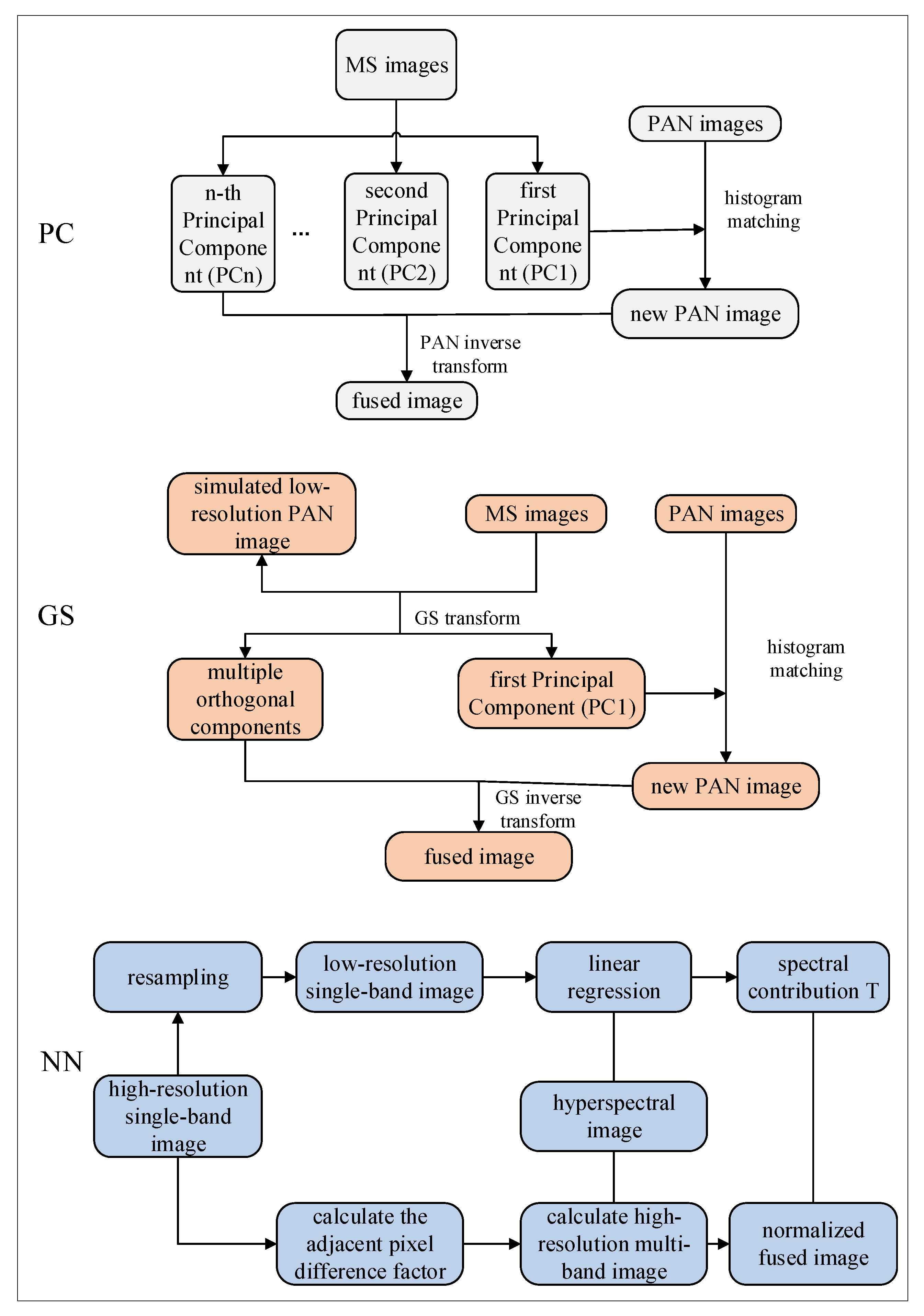
The PC fusion method improves multispectral images using high-resolution band-sharpening [32]. This procedure involves performing PC analysis on multispectral data from Landsat 8, GF-1, and Sentinel-2, followed by replacing the first PC with a high-resolution band [33]. After nearest-neighbor resampling, the inverse PC transformation was applied to achieve high-resolution pixel dimensions. The fusion image was obtained in the color space by applying a transformation using the eigenvector matrix of the covariance matrix, where the panchromatic image replaced the first component before the inverse transformation. GS fusion is a transformation-based method based on Schmidt orthogonalization [34]. Similar to the PC transformation, GS preserves the orthogonal relationships between components while minimizing information loss. During the GS transformation, the first component remained unchanged, facilitating interband inverse transformation through these orthogonal relationships. The NN fusion method, specifically the NN Diffuse Pan Sharpening technique proposed in 2014 [35], utilizes trained NNs to learn the transformation patterns between multispectral and panchromatic images. This approach generates high-resolution multispectral images that are then integrated with the original high-resolution panchromatic images. The NN method demonstrated exceptional flexibility and broad applicability across a wide range of image fusion tasks. The flowchart of the PC, GS, and NN algorithm is shown in Figure A1.

2.3.2. Sample Data Production

Training samples were systematically distributed across the study area. During the flowering period, numerous pure cotton and mixed pixels were observed along the field boundaries. After the MNF transformation, the Pixel Purity Index (PPI) was calculated to identify pure cotton pixels. Through iterative threshold optimization during model training, an optimal purity threshold of 5.6 was determined after 1000 iterations. Using high-resolution Google Earth imagery as a reference, 900 pure cotton pixels and 700 pure pixels from other crops were selected as the endmember training samples. Vegetated areas were identified by applying an NDVI threshold > 0.2. Cotton fields exhibited a distinctly dark green coloration compared with other croplands. Repeated visual verification and data processing produced regionally representative training samples that corresponded to the endmember quantities. The Jeffries–Matusita (J-M) distance was used to evaluate sample separability, offering advantages such as relaxed assumptions about data distribution and effective normalization for zero-mean data [36]. The selected samples exhibited high separability, with J-M distances ranging from 1.968 to 1.972, thereby meeting the criteria for accurate cotton field classification, as shown in

Table 3. Separability of cotton fields and other samples.

Number of Trials	Sample Endmembers	Regional Samples
1	1.971	1.969
2	1.972	1.968
3	1.971	1.968

.

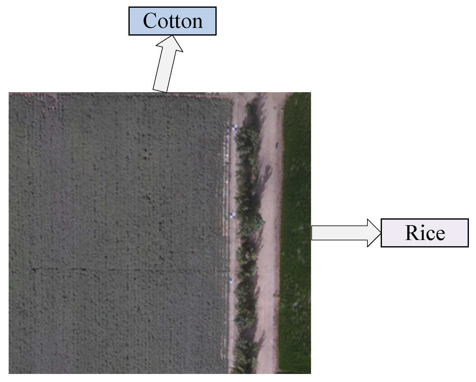
The quality of the sample dataset directly influences the performance of deep learning classifiers and, consequently, affects the classification accuracy. The required training sample set varied depending on the specific classification requirements. To maintain consistency with traditional supervised learning methods in data processing, this study adopted a customized approach for constructing the sample dataset, which primarily involved two key steps: (1) pre-processing the training images and (2) generating labeled datasets. During the training image pre-processing stage, Landsat 8 satellite imagery and fused images were segmented into 256 × 256-pixel patches to ensure a comprehensive representation of various land cover types across the study area. These image patches were systematically stored in two separate directories. An automatic labeling method based on empirical thresholds was implemented to generate labeled datasets while minimizing the annotation workload. The initial identification of the cotton fields was performed using an NDVI threshold of 0.5. Considering the potential interference of urban green spaces and other crops, manual corrections were applied to the initial results. Using ArcGIS 10.5 software, the raster data were converted into point vector data to facilitate subsequent editing operations, including the removal of misclassified points and the addition of omitted classification points. This process ensured the complete and accurate labeling of cotton fields [37]. The corrected point vector data were then converted into label-ready raster data using point-to-raster conversion tools. Using Python 3.6.4 scripting, the labeled images were cropped to dimensions of 256 × 256 pixels and saved in a dedicated label directory, thereby completing the construction of the labeled dataset. The dataset contained original images with four spectral bands (blue, red, green, and NIR), whereas the corresponding label images were single-channel grayscale maps with cotton fields marked as 1 and other areas as 0. The final dataset consisted of 729 training images and 683 prediction images in TIFF format. The processed imagery of the study area measured 1026 rows × 1062 columns covering approximately 108.96 km². Sample Set Creation is shown in Figure 2. The color difference between cotton and other crops (rice) is shown in Figure A2.

2.4. Model-Building Methods

2.4.1. GBDT Model

GBDT is a widely used machine learning algorithm that falls under the category of ensemble learning [38]. It improves the prediction accuracy by combining the outputs of multiple decision tree models. GBDT exhibits exceptional performance in addressing regression, classification, and various other tasks, particularly when dealing with complex, nonlinear datasets. The computational equation is given in Equation (1).

$$FT\left(x\right)=F_0\left(x\right)+\eta {\sum }_{t=1}^T{\sum }_{j=1}^{Jt}{\gamma }_{jt}I(x\in R_{jt})$$

(1)

where $FT\left(x\right)$ represents the model after the T-th iteration; $F_0\left(x\right)$ denotes the initial model; η indicates the learning rate; T signifies the number of iterations; $Jt$ is the number of leaf nodes in the t-th decision tree; ${\gamma }_{jt}$ refers to the weight of the j-th leaf node in the t-th decision tree; $R_{jt}$ represents the sample region corresponding to the j-th leaf node of the t-th decision tree, and $I(x\in R_{jt})$ is an indicator function that equals 1 when sample x falls within the region $R_{jt}$ and 0 otherwise.

2.4.2. MLC Model

The MLC emphasizes the statistical characteristics of the cluster distribution. Based on Bayesian principles, classification decisions rely on discriminant functions derived from the multivariate normal distributions for each category. The maximum likelihood estimation method achieves classification by constructing discriminant functions across all the image bands [39]. For each pixel to be classified, the probability of belonging to each known category is computed, and the pixel is assigned to the category with the highest probability. However, this method imposes stringent requirements on sample selection. If the population probability distribution of the selected samples deviates from a multivariate normal distribution, the accuracy of land-cover classification in remote sensing imagery may be adversely affected. The computational equation is given in Equation (2).

$${ g}_k(x_i)=-{\displaystyle \frac{1}{2}}ln(\sum k)-{\displaystyle \frac{1}{2}}{(x_i-m_k)}^T{(\sum k)}^{-1}(x_i-m_k)$$

(2)

where $g_k(x_i)$ denotes the discriminant function value for a pixel $x_i$ belonging to the k-th class; $\sum k$ represents the covariance matrix of the k-th class; $m_k$ indicates the mean vector of the k-th class; $x_i$ stands for the pixel vector to be classified, and T signifies matrix transposition.

2.4.3. RFC Model

An RFC performs classification or regression analysis by constructing multiple decision trees. This technique uses bootstrap sampling to extract numerous subsets from an original dataset. In the RFC, each subset serves as the basis for feature selection during the splitting process of individual subtrees. At each node split, a random subset of features is selected, and the optimal feature for splitting is determined from this subset. Subsequently, each tree is trained using the selected features. Ultimately, ensemble predictions are obtained by aggregating the outputs of all decision trees, either by majority voting or by averaging the predictions of individual trees [40].

2.4.4. PLSR Model

PLSR is a statistical method used to simultaneously model the relationships between the predictor variables (X) and response variables (Y). It is particularly useful in situations where the number of predictors exceeds the number of observations or when multicollinearity is present [41]. PLSR identifies latent relationships between predictors and responses, making it particularly popular in chemometrics, economics, and environmental sciences, particularly for analyzing spectral and high-dimensional datasets. The computational equation is as follows:

$$\widehat{Y}=({\displaystyle \frac{X-\mu x}{\sigma x}})W{(P\prime W)}^{-1}Q\prime +{\mu }_Y$$

(3)

where $\widehat{Y}$ is the predicted response variable matrix; $X$ represents the input predictor variable matrix; $\mu x$ denotes the mean vector of $X$; $\sigma x$ represents the standard deviation vector of $X$; $W$ is the weight matrix; $P$ and $Q$ are the loading matrices for the $X$-space and $Y$-space, respectively, and ${\mu }_Y$ signifies the mean vector of $Y$. This equation describes the prediction of response variables by multiplying the standardized predictor variables by a series of transformation matrices.

2.4.5. CBAM-ASPP-U-Net Model

U-Net represents an architectural paradigm distinct from Fully Convolutional Networks (FCNs), and demonstrates exceptional performance in image segmentation tasks, particularly in accurately delineating boundaries in cotton fields. Its structure maintains robust performance even with limited annotated data, making it particularly suitable for agricultural applications where data acquisition poses challenges [42]. The incorporation of skip connections facilitates the effective integration of deep and shallow features, thereby enhancing the model’s ability to discriminate features specific to cotton fields. The architectural innovation of U-Net lies in its encoder–decoder framework, which uses convolutional layers instead of traditional fully connected layers. This design provides flexibility in processing input images of varying sizes without the need for dimensional standardization, thereby significantly improving its practical applicability [43]. The ASPP module uses dilated convolutions with different sampling rates to capture multi-scale image information. This capability is particularly valuable for detecting cotton fields in remote sensing imagery, where the target objects exhibit considerable size and morphological variations. This enables better differentiation between cotton fields and other types of vegetation and land cover [44]. Dilated convolutions significantly expand the receptive field without incurring additional computational cost. The ASPP architecture addresses the information loss that often occurs during successive downsampling operations, which is a common limitation in traditional convolutional networks, using a synergistic combination of dilated convolutions and global average pooling. This approach effectively preserves essential spatial information [45]. CBAM improves the discriminative power of a network through dual-dimensional (channel and spatial) feature-weight optimization. Initially, the module spatially compresses the input feature maps to create two one-dimensional feature representations, which were then processed using a network structure consisting of hidden layers and multilayer perceptrons [46]. This process facilitates element-wise feature-map weighting and fusion, followed by the application of an activation function. By simultaneously considering both channel and spatial information for feature refinement, CBAM achieves a more effective resource reallocation with minimal computational and parametric overheads, thereby extracting more discriminative features. Its structural design facilitates focused attention on critical data dimensions, including depth, width, height, orientation, and positional relationships, which substantially improve the interpretative and analytical capabilities of this model. The software version used in the model is Pytorch 1.9.0 and CUDA10.2. The architecture of the CBAM-ASPP-U-Net network is illustrated in Figure 3.

2.5. Evaluation Indicators

2.5.1. Evaluation Index of Image Fusion

Image fusion quality assessment utilizes objective evaluation methods. These quantitative approaches use numerical metrics to characterize and evaluate the properties of fused images, offering advantages such as objectivity, precision, and automation. This methodology demonstrates fusion performance while minimizing the subjective biases that may result from the interpreter’s experience and external environmental factors in human evaluations. Three metrics were selected for assessment: the mean value (representing the average gray level of the image), standard deviation (indicating the variability of gray levels), and information entropy (reflecting the complexity of image information).

$$\mu ={\displaystyle \frac{{\sum }_{i=1}^M{\sum }_{j=1}^{N}F\left(i,j\right)}{M\times N}}$$

(4)

where $\mu$ represents the grayscale mean of the image; $F\left(i,j\right)$ denotes the grayscale value at the position $\left(i,j\right)$; M indicates the number of rows in the image, and N stands for the number of columns in the image.

$$std=\sqrt{{\displaystyle \frac{{\sum }_{m=1}^M{\sum }_{n=1}^N{(F\left(m,n\right)-\mu )}^2}{M\times N}}}$$

(5)

where std represents the grayscale standard deviation of the image; $F\left(m,n\right)$ denotes the grayscale value at the position $\left(m,n\right)$; $\mu$ is the grayscale mean of the image; M is the number of rows in the image, and N is the number of columns in the image.

$$H\left(x\right)=-{\sum }_{m=1}^M{p}_{i}ln{p}_i$$

(6)

where $H\left(x\right)$ is the information entropy of the image; $p_i$ is the probability of the occurrence of pixels with gray value i in the image, and m is the number of possible gray levels of the image.

2.5.2. Evaluation Index of Classification Model

The confusion matrix, also known as the error matrix, provides a standardized format for assessing accuracy using an n × n square matrix. The diagonal elements represent the number of correctly classified pixels. Four metrics were utilized: the kappa coefficient (classification accuracy), OA, user accuracy (UA), and producer accuracy (PA), all of which ranged from 0 to 1, with values > 0.8 indicating satisfactory extraction performance [47]. In this study, OA and kappa were used to evaluate the overall classification accuracy of cotton fields, whereas UA and PA quantified the commission and omission errors, respectively. The Mean Intersection over Union (MIoU) measures the model’s average degree of overlap, with higher values indicating superior performance. The mAP@0.5 assessed the overall performance of the model at this specified threshold.

$$K_{hat}={\displaystyle \frac{N{\sum }_{i=1}^r{x}_{ii-}{\sum }_{i=1}^r(x_{i+}{x}_{+i})}{N^2-{\sum }_{i=1}^r(x_{i+}{x}_{+i})}}$$

(7)

where $K_{hat}$ denotes the kappa coefficient; N represents the total number of samples; r indicates the number of classification categories; ${\chi }_{ii}$ refers to the element values on the main diagonal of the confusion matrix; $x_{i+}$ stands for the sum of the ith row in the confusion matrix, and $x_{+i}$ represents the sum of the ith column in the confusion matrix.

$$P_C=\sum _{k=1}^q{p}_{kk}/p$$

(8)

where $P_C$ represents the OA; $p_{kk}$ denotes the element values on the main diagonal of the confusion matrix; p indicates the total number of samples, and q stands for the number of classification categories.

$$p_{ui}=p_{ii}/p_{i+}$$

(9)

where $p_{ui}$ represents the user’s accuracy; $p_{ii}$ denotes the element value on the main diagonal of the confusion matrix, and $p_{i+}$ indicates the sum of the ith row in the confusion matrix.

$$PA={\displaystyle \frac{\sum _{i=1}^{n}T{P}_j+T{N}_j}{\sum _{i=1}^{n}T{P}_j+F{P}_j+F{N}_j+T{N}_j+F{N}_j}}$$

(10)

where PA represents the producer’s accuracy; $T{P}_j$ denotes the true positive count for class j; $T{N}_j$ indicates the true negative count for class j; $F{P}_j$ stands for the false positive count for class j; $F{N}_j$ refers to the false negative count for class j, and n represents the number of classification categories.

$$MIoU={\displaystyle \frac{1}{N}}\sum _{j=1}^n{\displaystyle \frac{\sum _{i=1}^{n}T{P}_j+T{N}_j}{T{P}_j+F{P}_j+F{N}_j}}$$

(11)

$MIoU$ represents the Mean Intersection over Union; N denotes the number of classes; $T{P}_j$ indicates the true positive count for class j; $T{N}_j$ refers to the true negative count for class j; FP_j represents the false positive count for class j; $F{N}_j$ stands for the false negative count for class j, and n signifies the number of classification categories.

$$mAP@0.5={\displaystyle \frac{1}{N}}\sum _{j=1}^{n}A{P}_j$$

(12)

where mAP@0.5 represents the mean average precision at an IoU threshold of 0.5; N denotes the number of categories; $A{P}_j$ indicates the average precision for the i-th class, and n stands for the total number of classification categories.

3. Results

3.1. Fusion Image Results Analysis

In this study, multi-feature fusion of GF-1, Sentinel-2, and Landsat 8 imagery was performed using a two-step process. Initially, the panchromatic band from Landsat 8’s OLI sensor was fused with its 30 m resolution multispectral bands to improve spatial resolution while preserving spectral information. Subsequently, three fusion methods (PC, GS, and NN) were compared, enabling a clear differentiation from the original single-sensor images. A quantitative evaluation was conducted using objective metrics, including mean value, standard deviation, and information entropy, to identify the optimal fusion performance.

3.1.1. Multi-Feature-Based Fusion Image Evaluation

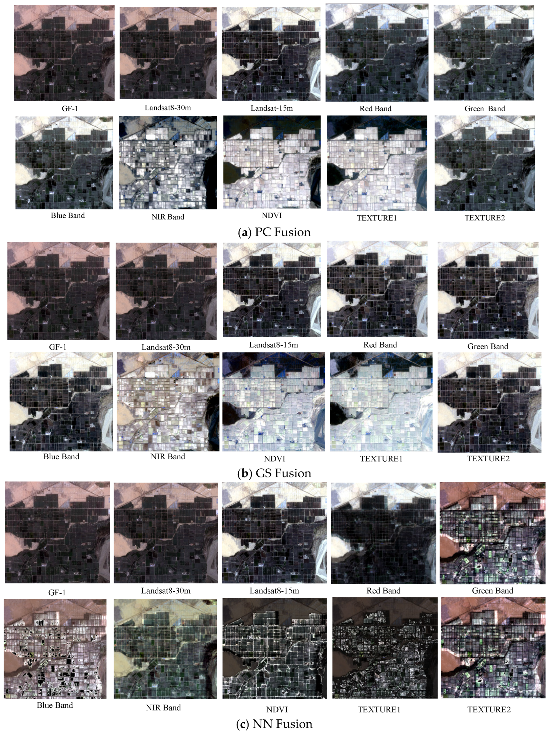
Figure A3 illustrates the feature fusion mapping results of the seven combinations using GF-1 and Landsat 8 imagery. Both the original GF-1 and Landsat 8 (30 m) images exhibited relatively dark tones with indistinct field boundaries, whereas the pan-sharpened Landsat 8 imagery exhibited a significant quality improvement. Specifically, the GS-fused blue, green, red, and TEXTURE2 bands incorporated additional spectral information from Landsat 8’s panchromatic band compared with the original GF-1 imagery, resulting in improved information richness. Compared with the two original Landsat 8 images, the fused products exhibited improved texture representation of field boundaries and better contrast for small plots, therefore enabling a more accurate extraction of cotton fields. In terms of fusion methods, both PC and GS outperformed the NN in terms of overall performance. For the PC and GS methods, the blue, green, and red bands retained information that was comparable to that of the original imagery, exhibiting minimal visual differences. In contrast, the NIR band exhibited color inconsistencies in cotton fields, appearing grayish–white and exhibiting significant spectral distortions. NDVI imagery effectively suppressed non-vegetated targets while enhancing spectral variations in vegetation, thus highlighting cultivated areas. The results from TEXTURE1 were similar to those of NDVI, but exhibited color distortion, which hindered the identification of cotton fields. This issue was attributed to the similar 16 m resolution of the GF-1 and Landsat 8 sensors, which resulted in insufficient interpixel variation for effective NN-based linear regression. A detailed comparison indicated that GS fusion offered superior spatial and color representation with clearer inter-feature textures than PC fusion, thereby facilitating a more intuitive visual interpretation. However, despite the clear delineation of field boundaries, the GS-fused NIR band exhibited spectral distortions that could result in omission errors during cotton field extraction. Both GS-NDVI and TEXTURE1 overemphasized vegetation by producing a homogeneous tonal representation, which increased the risk of commission errors in identifying cotton fields.

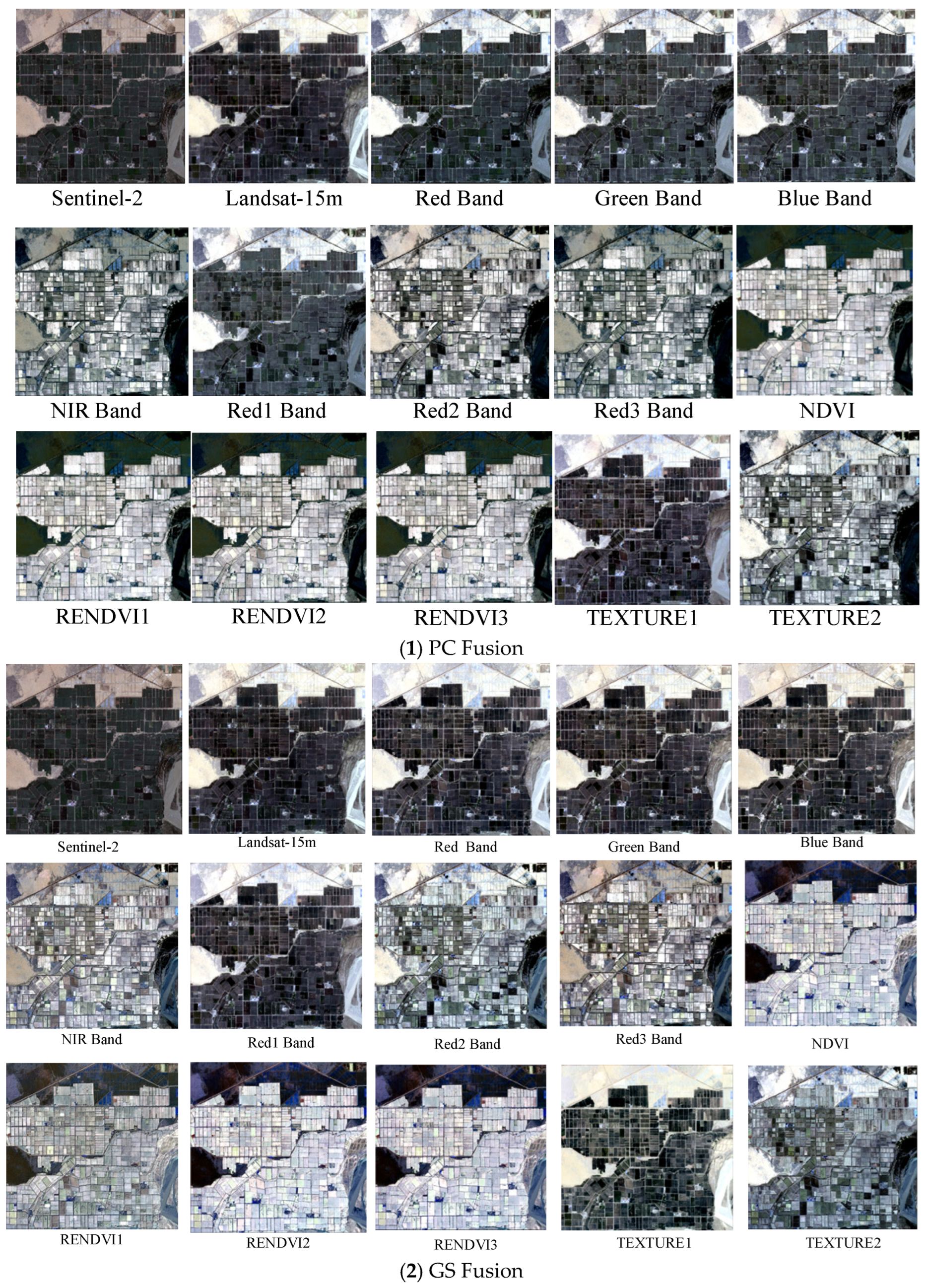
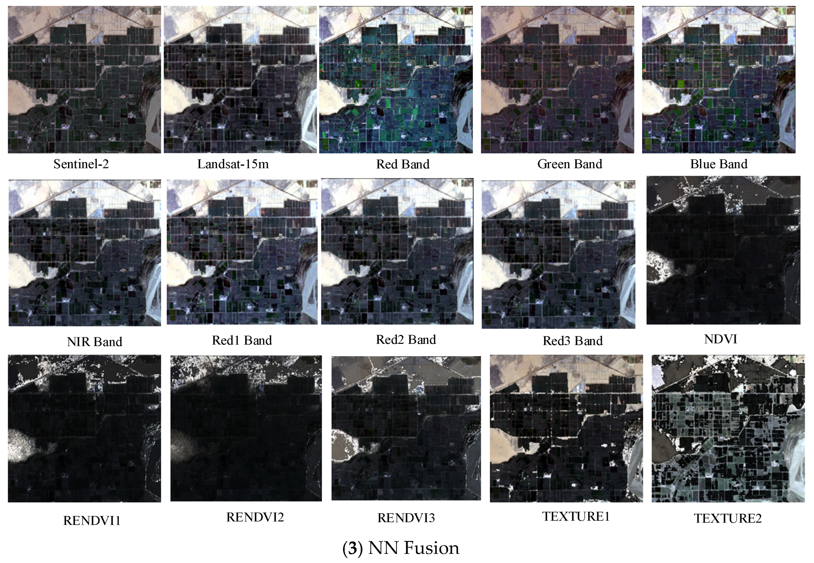
As illustrated in Figure A4, the fusion of Sentinel-2 and Landsat 8 exhibited spectral distortion. The subjective evaluation ranked the fusion performance as follows: NN (7) > PC (5) > GS (4), where the numbers represent the number of features (out of 13 fused features) that closely resemble the original images. The NN method effectively integrated the spectral characteristics of Sentinel-2 and Landsat 8 data, producing seven-band images that were rich in spatial information and distinct textural features. However, the two texture feature images exhibited spectral distortion, and the four vegetation indices exhibited improved salt-and-pepper noise. Both the PC and GS methods successfully fused the Sentinel-2 blue, green, red, and red-edge 1 bands with the Landsat 8 data. In contrast, the red edge 2, red edge 3, and NIR bands, along with four vegetation index features, exhibited fusion qualities similar to those observed in the GF-1 results, resulting in either color loss or blurred textures. The PC-TEXTURE1 fusion achieved an image quality close to the original, whereas the other three texture features exhibited color loss. Remarkably, TEXTURE1 consistently outperformed TEXTURE2 across all three fusion methods, which can be attributed to the MNF transformation concentrating more information on TEXTURE1. Given the substantial number of well-fused band features in Sentinel-2 and Landsat 8 combinations, as well as the challenges associated with visual differentiation, the optimal fusion method was selected through an objective quantitative evaluation.

Table 4. Objective evaluation of fusion results.

Satellite Fusion	Quantitative Evaluation	Mean			Standard Deviation			Information Entropy
	Fusion Bands	PC	GS	NN	PC	GS	NN	PC	GS	NN
GF-1 fused with Landsat8 features	Blue band	6286	6278	31,371	2126	2297	19,786	8.51	8.52	8.57
	Green band	6285	6277	25,526	2128	2290	13,566	8.51	8.54	8.64
	Red band	6283	6289	6305	2131	2294	3370	8.46	8.5	8.45
	NIR band	6207	6282	6312	1832	1630	1980	8.15	8.46	8.39
	NDVI	6318	6285	15,806	2116	1782	13,015	8.34	8.47	8.6
	TEXTURE1	6288	6285	13,587	2124	1866	15,000	8.28	8.46	8.51
	TEXTURE2	6285	6285	25,527	2128	2284	13,567	8.51	8.54	8.64
Sentinel-2 fused with Landsat8 features	Blue band	6287	16,725	14,720	2117	2290	4764	8.53	8.55	8.59
	Green band	6288	6276	13,464	2119	2286	4230	8.51	8.54	8.56
	Red band	6283	6278	12,628	2126	2297	4438	8.46	8.51	8.57
	Red edge 1 band	6286	6276	10,324	2118	2263	3147	8.45	8.62	8.45
	Red edge 2 band	6356	6283	7058	1905	1729	2420	8.3	8.48	8.39
	Red edge 3 band	6353	6280	7050	1922	1634	2485	8.28	8.49	8.39
	NIR band	6354	6281	6928	1930	1653	2453	8.31	8.55	8.48
	NDVI	6295	6284	8684	2104	1745	11,590	8.36	8.51	8.49
	RENDVI1	6295	6289	11,642	2103	1818	17,125	8.37	8.62	8.61
	RENDVI2	6294	6284	8922	2107	1739	13,683	8.4	8.52	8.51
	RENDVI3	9293	6284	8052	2109	1745	9121	8.4	8.5	8.47
	TEXTURE1	6281	6296	7486	2122	2343	6237	8.47	8.34	8.21
	TEXTURE2	6353	6298	3079	1913	1745	2263	8.3	8.5	8.27

presents the objective evaluation results, in which the mean value represents the image brightness, whereas the standard deviation and information entropy characterize the spatial information. The highest mean value recorded was 31,371 for the NN-blue band fusion using GF-1, whereas the lowest value was 3079 for the NN-TEXTURE2 fusion using Sentinel-2. After excluding these extreme values, the mean values ranged from 6207 to 25,527. Further elimination of subjectively identified anomalous images revealed that GS-blue band fusion with Sentinel-2 exhibited the highest mean value of 16,725, indicating optimal brightness characteristics. Regarding spatial information (post-extreme-value removal and subjective filtering), Sentinel-2’s NN method demonstrated superior performance across the seven spectral bands, achieving the highest standard deviation of 4764 (NN-blue band), which reflects rich tonal variation and improved spatial information. The PC fusion demonstrated a stable contrast performance, with standard deviations ranging from 1913 to 2128; however, these values were generally lower than those observed with the NN method. Remarkably, all three fusion methods maintained consistent information entropy values (ranging from 8.15 to 8.62) for both GF-1 and Sentinel-2 images when fused with Landsat 8, confirming the methodological robustness of the image fusion. Comprehensive subjective and objective evaluations indicated that the optimal image fusion method in this study was GS-blue band fusion between Sentinel-2 and Landsat 8, which yielded a mean value of 16,725, standard deviation of 2290, and information entropy of 8.55. The GS-blue band-fused imagery exhibited high brightness, distinct textural features, and exceptional spatial details. The significant spectral differences between the cotton fields and other crop areas in the fused images facilitated their preliminary identification.

3.1.2. Comparative Analysis of Optimal Fusion and Single-Source Image Quality

Table 5. Objective evaluation of GS-blue wave segment and single-source image.

Data	Resolution	Mean	Standard Deviation	Information Entropy
GF-1	16	7076	2070	7.61
Sentinel-2	10	9226	2244	8.13
Landsat8 raw data	30	6196	2122	8.27
Landsat8 full color	15	6284	2154	8.51
GS-blue band	10	16,725	2290	8.55

presents a comparative analysis of the single-sensor imagery and the optimal fusion of the GS-blue bands from Sentinel-2 and Landsat 8. The results indicated that pan-sharpened Landsat 8 imagery exhibited marginal improvements in mean value, standard deviation, and information entropy, with increases of 88, 32, and 0, respectively. In contrast, the GS-blue band fusion achieved significant improvements over the original Landsat 8 imagery, with improvements of 10,529, 168, and 0.28, respectively. Compared with Sentinel-2, the fusion resulted in increases of 7499, 46, and 0.42, whereas relative to the GF-1 WFV imagery, the improvements reached 9649, 220, and 0.94, respectively. The GS-blue band fusion effectively integrated the advantages of both Sentinel-2 and Landsat 8, demonstrating significant improvements in brightness information and moderate improvements in spatial resolution. This establishes a theoretical foundation for the subsequent extraction and classification of cotton fields.

3.2. Identification Results and Analysis of Cotton Fields Based on Region and Endmember Sample Selection Method

The classification accuracy was significantly influenced by the number of training samples. Studies have shown that the optimal sample size typically ranges from 24 to 30 times the number of selected image bands. However, the required training sample size also depends on the extent of the study area, the complexity of land cover types, and the classification methods used. To verify the stability of the experimental results, stratified random sampling was implemented by selecting subsets of 50, 100, 150, 200, 250, and 300 cotton samples from both endmember and regional sample libraries. These subsets were used to test five supervised classifiers for cotton-field extraction in the Alar Reclamation zone. Three independent trials were conducted for each sample size to mitigate the bias caused by sample randomness, resulting in 324 classified images across all the classifiers. Finally, the classification results were statistically evaluated using validation sample sets.

3.2.1. Single-Factor Model Construction

(1)

Positional accuracy and classification error analyses

As shown in

Table 6. Comparison of model accuracy under different algorithms and samples.

Algorithmic Model	Sample Size	UA (%)		PA (%)		OA (%)		KAPPA (%)
		Sample Endmembers	Regional Samples	Sample Endmembers	Regional Samples	Sample Endmembers	Regional Samples	Sample Endmembers	Regional Samples
GBDT	50	85.05	84.99	93.04	93.04	83.69	83.43	0.881	0.895
	100	84.69	84.63	90.99	90.99	87.13	86.87	0.917	0.931
	150	84.63	84.57	94.59	94.59	88.51	88.25	0.921	0.935
	200	84.46	84.4	94.55	94.55	89.40	89.14	0.927	0.941
	250	84.49	84.43	94.57	94.57	88.34	88.08	0.919	0.933
	300	84.65	84.59	94.59	94.59	93.50	93.24	0.927	0.941
MLC	50	91.15	94.08	95.05	96.51	94.88	97.12	0.907	0.951
	100	90.02	94.05	95.02	96.66	94.38	97.02	0.897	0.949
	150	93.79	94.06	95.63	96.64	96.28	97.02	0.935	0.949
	200	93.98	94.27	95.59	96.66	96.38	97.12	0.937	0.951
	250	93.37	94.13	95.09	95.76	96.38	97.12	0.937	0.951
	300	94.76	94.28	94.91	96.68	96.58	97.02	0.941	0.949
RFC	50	90.24	95.63	93.11	91.68	94.38	94.62	0.907	0.91
	100	90.03	96.02	96.22	92.66	94.28	95.12	0.905	0.916
	150	95.13	95.83	95.31	92.92	96.98	95.22	0.959	0.929
	200	97.13	97.12	96.89	92.91	97.28	95.32	0.961	0.951
	250	96.23	95.25	97.11	96.57	97.08	97.12	0.961	0.963
	300	95.43	95.44	95.29	97.09	97.08	97.22	0.961	0.963
PLSR	50	88.20	88.15	92.17	92.26	86.78	86.65	0.917	0.921
	100	87.70	87.65	91.04	91.13	86.48	86.29	0.894	0.899
	150	89.60	89.55	94.81	94.89	86.38	86.23	0.919	0.921
	200	89.70	89.65	95.01	95.09	86.32	86.06	0.929	0.931
	250	89.70	89.65	94.39	94.48	86.38	86.09	0.932	0.937
	300	89.90	89.85	95.78	95.87	86.98	86.25	0.932	0.937
U-Net	50	89.19	87.04	92.57	94.13	84.67	84.41	0.856	0.834
	100	88.79	89.14	90.47	92.03	83.54	83.28	0.898	0.876
	150	89.79	89.94	94.12	95.68	87.31	87.05	0.884	0.892
	200	90.19	90.44	93.96	95.71	87.50	87.24	0.894	0.902
	250	89.89	90.84	94.05	95.74	86.89	86.63	0.892	0.890
	300	90.69	92.64	94.09	95.83	88.28	88.22	0.908	0.906

, the maximum kappa value for the endmember samples was 0.963, with an OA of 97.22%. In contrast, the highest kappa value for the regional samples was 0.961, with an OA of 97.18%, indicating minimal differences between the two types of samples. For the endmember samples, the performance ranges of the GBDT, MLC, RFC, PLSR, and U-Net were 0.881–0.927, 0.907–0.951, 0.905–0.963, 0.894–0.932, and 0.856–0.948, respectively. GBDT was less affected by sample size, whereas the RFC was highly sensitive. In regional samples, the ranges for GBDT, MLC, RFC, PLSR, and U-Net were 0.895–0.941, 0.949–0.951, 0.912–0.961, 0.907–0.945, and 0.834–0.946, respectively. The MLC and U-Net models were less affected by sample size, whereas the RFC remained highly sensitive. Among all classifiers, RFC achieved the best performance with endmember sample sizes of 250 and 300, yielding a kappa coefficient of 0.963 and an OA of 97.22%. The training process for RFC is complex and requires a substantial number of samples to achieve optimal performance, particularly for sample sizes of 200, 250, and 300. The RFC selects candidate features for subtree splitting during the construction of the subset datasets. Combined with the extensive cotton cultivation area in the Aral reclamation zone and the unique spectral characteristics of cotton during the boll-opening period, RFC achieved optimal classification accuracy with an adequate number of samples. In the endmember samples, the RFC demonstrated the highest UA curve, peaking at 97.13% (with a sample size of 200) and reaching a minimum of 90.03% (with a sample size of 100). UA of the RFC increased significantly with larger sample sizes, which was consistent with its inherent characteristics. In contrast to RFC and U-Net, the other classifiers demonstrated stable performance curves with minimal sensitivity to sample size. For regional samples, the UA ranged from 84.4% to 97.12%. Compared with the endmember samples, the misclassification of cotton fields was more pronounced under mixed-pixel conditions. In the endmember samples, the PA ranged from 88.51% to 97.09%, with the RFC achieving the highest value of 97.09% using 300 training samples. For the regional samples, the PA ranged from 90.99% to 97.11%. The PA values for the regional samples were higher than those for the endmember samples because pure pixels failed to capture some pest-affected cotton, and unharvested cotton was overlooked during the feature calculation. By contrast, mixed pixels contain multiple reference factors that effectively reduce the number of misclassified pixels. Comparative analysis revealed that RFC exhibited lower misclassification rates in both endmember and regional samples, outperforming the other classifiers. Although the RFC exhibited minimal misclassifications in the endmember samples, its performance declined with smaller regional sample sizes and improved only after exceeding 250 samples.

(2)

Accuracy analysis of total number of regions

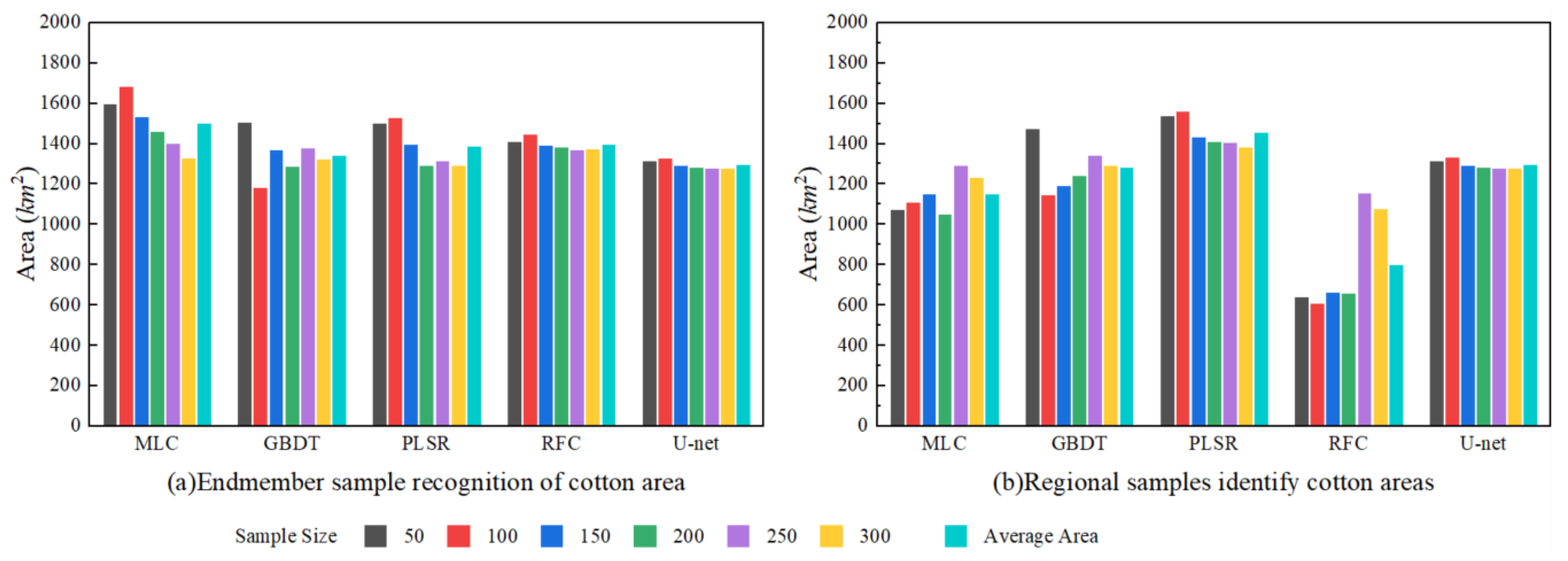
As illustrated in Figure 4, the cotton field area in the endmember samples ranged from 686.24 to 1779.38 km², with a mean value between 780.65 and 1726.62 km². In contrast, the regional samples ranged from 679.89 to 1819.11 km², with a mean between 731.79 and 1673.1 km², indicating a close agreement between the two sample types. This study revealed significant discrepancies in cotton field extraction across various classifiers. With a regional sample size of 50, RFC extracted 679.89 km², whereas MLC extracted 1819.11 km², resulting in a substantial difference of 1139.55 km². For the same classifier with different sample sizes, the RFC estimated a cotton field area of 1401.45 km² using 200 endmember samples, which was closest to the actual cotton field area in the Aral reclamation zone (2.05 million mu, or 1366.67 km²). This value differed by 63.49 km² from the 1424.94 km² obtained using 100 endmember samples, indicating that the RFC exhibited the largest deviation at 12–25 times the band count, while performing closest to the actual value at 12–75 times the band count. Using the same classifier and sample size, a comparison between endmember and regional samples revealed that the mean RFC extraction in endmember samples (1375.3 km²) was significantly higher than that in regional samples (787.6 km²). This discrepancy indicates a poor performance in mixed-pixel environments and difficulties in extracting precise information from homogeneous regions. In contrast, PLSR yielded a mean area of 1395.63 km² in the regional samples, which was lower than the 1551.32 km² observed in the endmember samples; however, its values across different sample sizes remained close to the actual area. Comparative analysis demonstrated that the five classifiers exhibited distinct characteristics for the extraction of cotton fields. RFC was performed accurately on the endmember samples, demonstrating consistent extraction at sample sizes of 200, 250, and 300. Nevertheless, in practice, highly pure pixels are rare, and intercropping within cotton fields is common. Therefore, deep learning methods for multi-scale feature extraction can significantly improve the accuracy of cotton field mapping.

3.2.2. Multi-Factor Model Construction Based on CBAM-ASPP-U-Net

As illustrated in Figure 5, a comparison of the three deep learning methods using identical training approaches revealed that CBAM-ASPP-U-Net achieved the highest mAP@0.5 value of 0.973 and the highest MIoU of 0.983. This demonstrates its superior average accuracy and effectiveness for extracting cotton fields. The ASPP-U-Net achieved maximum values of 0.947 for mAP@0.5 and 0.961 for MIoU, representing improvements of 0.026 and 0.022, respectively, compared with the CBAM-enhanced model. The integration of various modules significantly improved the average accuracy of the U-Net, confirming its enhanced applicability to cotton field extraction tasks.

As shown in

Table 7. Comparison of the accuracy of ASPP-U-Net and CBAM-ASPP-U-Net under different samples.

Algorithmic Model	Sample Size	UA (%)		PA (%)		OA (%)		KAPPA(%)
		Sample Endmembers	Regional Samples	Sample Endmembers	Regional Samples	Sample Endmembers	Regional Samples	Sample Endmembers	Regional Samples
ASPP-U-Net	50	86.13	84.99	93.04	89.42	83.69	83.43	0.881	0.895
	100	85.77	84.63	90.99	87.73	87.13	86.87	0.917	0.931
	150	85.71	84.57	94.59	91.37	88.51	88.25	0.921	0.935
	200	85.54	84.4	94.55	91.21	89.40	89.14	0.927	0.941
	250	85.57	84.43	94.57	92.61	88.34	88.08	0.919	0.933
	300	85.73	84.59	94.59	93.26	93.50	93.24	0.927	0.941
CBAM-ASPP-U-Net	50	91.15	94.08	95.05	96.51	94.88	97.12	0.907	0.951
	100	90.02	94.05	95.02	96.66	94.38	97.02	0.897	0.949
	150	93.79	94.06	95.63	96.64	96.28	97.02	0.935	0.949
	200	93.98	94.27	95.59	96.66	96.38	97.12	0.937	0.951
	250	93.37	94.13	95.09	95.76	96.38	97.12	0.937	0.951
	300	94.76	94.28	94.91	96.68	96.58	97.02	0.941	0.949

, CBAM-ASPP-U-Net achieved a kappa coefficient of 0.963 and an OA of 97.22% for the endmember samples. In comparison, the maximum kappa and OA values for the regional samples were 0.961 and 97.18%, respectively, indicating minimal differences between the two sample types. Similarly, ASPP-U-Net achieved a kappa of 0.963 and an OA of 97.22% for the endmember samples, with regional samples reaching maximum values of 0.961 (kappa) and 97.18% (OA), again demonstrating negligible variation between the sample types. CBAM-ASPP-U-Net predicted a cotton field area of 1341.25 km², which was slightly lower than the actual area of 1366.67 km². In contrast, RFC overestimated the area by 38.58 km² (1405.25 km² vs. 1366.67 km²). This discrepancy arises because the RFC has difficulty distinguishing cotton fields from intercropped regions, often misclassifying other crops as cotton, leading to overgeneralization. Although traditional machine learning methods demonstrate inferior evaluation metrics compared with deep learning, their spatial mapping results show only minor differences. Deep learning, with its distinctive sample training configuration, is particularly well-suited for multi-temporal analyses and scenarios that require fine-scale extraction of cotton fields.

3.2.3. Comparison of the Estimation Accuracy of Different Modeling Methods

(1)

Mapping and analysis of the spatial distribution of fused images

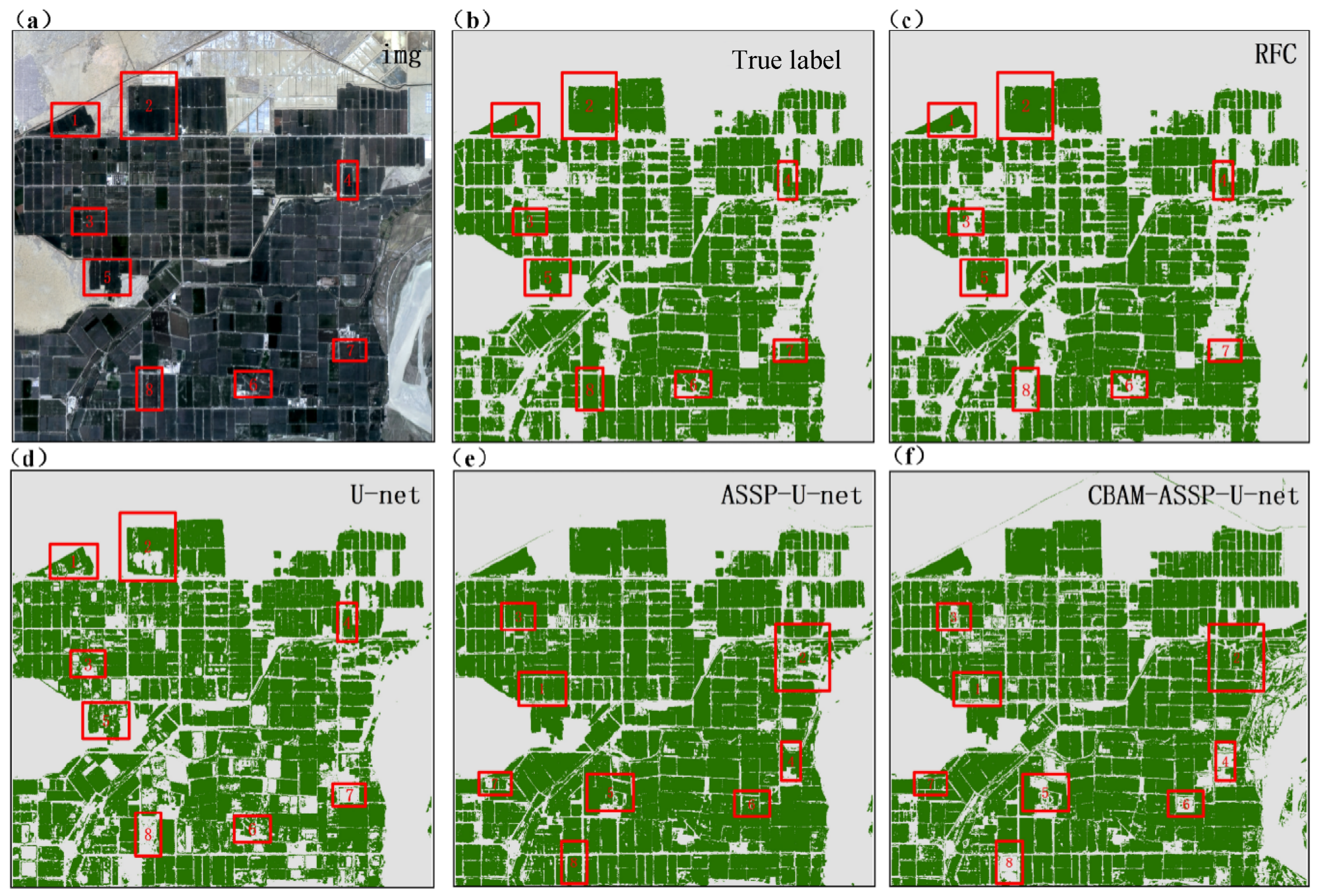
Figure 6 presents a comparative analysis of the cotton field extraction results obtained from various models using original Landsat 8 imagery. The ASPP model generated more complete cotton field parcels, whereas the U-Net output generated more blank regions. Through the visual interpretation of Google Earth imagery in complex cotton cultivation areas (regions 2, 7, and 8), the U-Net exhibited significant omission errors. These regions represent mixed cultivation areas, where cotton is grown alongside other crops. Although the ASPP model classified all three regions as cotton fields, some inaccuracies were present. Although cotton was predominant in these areas, it was accurately represented by dotted or linear patterns. In marked regions 1, 3, 5, and 6 (experimental fields under various disease stresses), the U-Net produced more fragmented, dotted-linear outputs than ASPP. Multi-source image fusion utilized satellite imagery captured during the cotton boll-opening period when diseased fields exhibited significant defoliation. Consequently, these areas remained cotton fields that the U-Net failed to fully extract, demonstrating its inferior interpretative capability compared with ASPP. Marked region 4, representing cotton fields surrounded by other crops, was successfully extracted using both the U-Net and ASPP models.

Figure 7 presents an analysis of cotton field extraction using the GS blue band. Both CBAM-ASPP-U-Net and ASPP-U-Net demonstrated a strong ability to extract information, producing results that accurately represent the spatial distribution of cotton fields. However, in regions 1, 3, and 5, the ASPP model exhibited misclassification. A comparison with Google Earth imagery revealed that these areas contained intercropped fields where cotton was grown alongside other crops. The interwoven planting patterns and similar spectral reflectance characteristics among different crops, coupled with the indistinct features of mixed cotton fields in 10 m resolution imagery, contribute to the misclassifications observed with the ASPP model. The ASPP model exhibited omission errors in Regions 2 and 7. Visual interpretation of Google Earth imagery indicated that these areas were affected by Verticillium wilt, which caused leaf drop and abnormal boll opening, resulting in loss of the most typical image features. In contrast, the dual attention mechanism of the CBAM model can automatically acquire and integrate advanced features to learn detailed image information, demonstrating superior performance in cotton field extraction compared with the ASPP model.

(2)

Accuracy analysis of the total amount in the region

As shown in

Table 8. Comparison of results from multiple algorithms.

		Kappa	OA (%)	UA (%)	PA (%)	Area (km2)	Office Area (km2)
RFC	GF-1	0.862	86.6	86.17	86.41	561.20	1366.67
	Landsat 8–30 m	0.865	89.77	89.56	89.56	645.12
	Sentinel-2	0.914	92.21	91.02	91.41	1530.94
	Landsat 8–15 m	0.911	91.86	86.74	85.98	1174.84
	GS-blue band	0.963	97.22	97.13	97.09	1405.25
ASPP-U-Net	Landsat 8–15 m	0.922	81.11	85.96	83.55	1565.45
	GS-blue band	0.976	97.36	96.99	97.88	1381.20
CBAM-ASPP-U-Net	Landsat 8–15 m	0.932	82.11	86.96	85.55	1620.66
	GS-blue band	0.988	98.56	98.99	100	1341.25

, the fused GS-blue band imagery from Sentinel-2 and Landsat 8 demonstrated outstanding performance, yielding a kappa value of 0.963, OA of 97.22%, UA of 97.13%, PA of 97.09%, and a cotton field extraction area of 1405.25 km². All of these metrics exceeded those obtained from single-source imagery. Although the GS-blue band exhibited results comparable to those of Sentinel-2 alone, it demonstrated significant improvements over Landsat 8 imagery, with increases of 0.098, 7.45%, 7.57%, and 7.53% for kappa, OA, UA, and PA, respectively. The GS-blue band significantly improved the accuracy of cotton field classification in traditional supervised learning approaches, demonstrating a marked improvement in data quality compared with the original datasets.

3.3. CBAM-ASPP-U-Net with RFC Mapping Analysis of Cotton Fields in Alar

The spatial mapping of cotton-field extraction using the optimal deep learning and machine learning methods is illustrated in Figure 8. A comparative analysis between the RFC and CBAM-ASPP-U-Net models revealed that the latter outperformed the former, achieving superior performance metrics (kappa = 0.988, OA = 98.56%, UA = 98.99%, and PA = 100%) compared with RFC. However, visual examination of the spatial maps indicated that both methods demonstrated comparable classification quality, with each exhibiting adequate spatial information representation and clear boundary delineation. The mapping results effectively illustrated the distribution of cotton fields throughout the Alar Reclamation in all cardinal directions, providing decision-makers with reliable spatial references for cultivation planning and management.

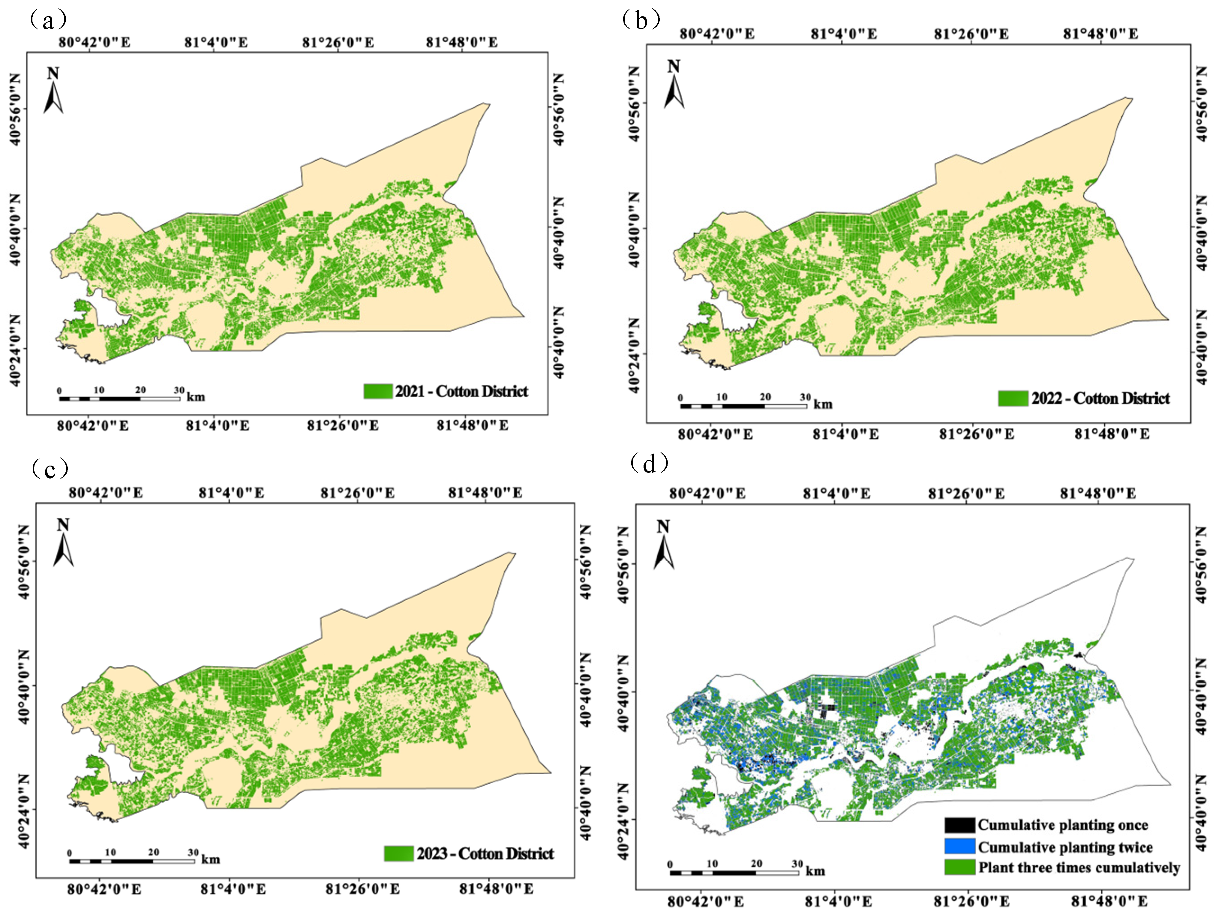
Satellite-derived mapping of the Alar Reclamation zone for 2021 and 2022 demonstrated consistent performance in cotton field extraction throughout the two-year study period (Figure 9), with no significant spatial distortions observed. The maps revealed consistent spatial patterns, showing the highest density of cotton fields in the mid-western Tarim River region, with progressively sparser cultivation in the eastern areas. Interannual variations in the spatial distribution patterns were minimal, showing no discernible differences in the mapped outputs.

To comprehensively analyze the interannual variations in cotton fields within the reclamation zone, we calculated and compared the predicted and observed cotton field areas over three consecutive years (Figure 10). The results demonstrated a close agreement between the predicted and actual areas in 2023, with a discrepancy of 25.42 km². In contrast, a larger deviation of 154.08 km² was observed in 2022. Although multiple factors, including cultivation practices, could account for the discrepancy in 2022, this study specifically attributed the variation to sample selection strategies and the potential influences from different deep-learning parameter configurations. The superimposition of optimal algorithm-derived cotton field maps from 2021 to 2023 revealed three distinct cultivation patterns: (1) the majority of fields exhibited continuous cultivation for ≥3 years; (2) two-year consecutive cultivation was concentrated in the central–western regions; and (3) minimal areas, which were spatially dispersed, were cultivated for only one year. A quantitative analysis of three years of continuous cultivation revealed field sizes ranging from 0.1 km² (n = 33,654 fields) to 12 km² (n = 112 fields), with the largest continuous cultivation area observed in central Alar.

4. Discussion

In agricultural remote sensing applications, multi-satellite data fusion technology offers comprehensive and accurate information and plays a significant role in crop monitoring and yield prediction. In this study, GF-1 and Sentinel-2 data were selected for fusion with the Landsat 8 imagery. Three fusion methods (PC, GS, and NN) were used to fuse the spectral characteristics, vegetation indices, and texture features of single-source satellite imagery. Fused imagery combining the GS-blue band of Sentinel-2 with that of Landsat 8 demonstrated superior performance in terms of both color representation and information content. In particular, spectral feature fusion significantly improved the clarity and color contrast of cotton-field images compared with the other methods. During the fusion of Sentinel-2 and Landsat 8, significant improvements were observed in mean, standard deviation, and information entropy. The fused imagery demonstrated clear advantages over single-source images for the accurate extraction of cotton fields. The results of this study demonstrated that the fusion of two satellite datasets yielded better outcomes than single-satellite data, which is consistent with the findings of Ram [48], who reported superior vegetation mapping results in Japan using fused Sentinel-2 and Landsat 8 data compared with single-satellite approaches. Li et al. [49] found that using advanced remote sensing algorithms and various fusion data for growing stock volume estimation, the fusion image data based on GF-2 and Sentinel-2 can effectively couple the advantages of the two and significantly improve the estimation performance of growing stock volume.

The endmember- and region-based sample extraction methods significantly improved the classification accuracy of machine learning classifiers. The four machine learning models exhibited minimal differences in kappa and OA values between the two sample types. Among all classifiers, RFC demonstrated optimal performance with endmember sample sizes of 250 and 300, achieving a kappa value of 0.963 and an OA of 97.22% (0.961 and 97.18%, respectively, for the regional samples). UA and PA metrics for the RFC model with 250 samples were 97.13% and 97.09%, respectively, successfully extracting a cotton field area of 1405.25 km². Although Hu [16] achieved 89.4% OA in cotton classification within the framework of multi-crops, we improved the accuracy to 97.22% by optimizing the key methods of sample selection. The improvement of 7.82% showed that the crop-specific sample strategies (endmember/region) are better than general random sampling. When the purity of the sample is ensured, RF becomes very important. These results underscore the importance of high-quality samples in enhancing the accuracy of cotton identification.

To enhance the U-Net model, this study incorporated the CBAM and ASPP modules, resulting in the CBAM-ASPP-U-Net model. When applied to cotton identification using GS-blue band images fused from Sentinel-2 and Landsat 8 data, this improved model demonstrated superior performance compared with the original U-Net, achieving higher values for kappa (0.988), OA (98.56%), UA (98.99%), and PA (100%). CBAM-ASPP-U-Net achieved 98.56% OA in cotton mapping, surpassing Seydi et al.’s [23] time-series CNN (95.2%). Our spatial attention method performs well in the case of mixed pixels (PA = 100% versus 92.8%), which proves that GS band fusion is superior to time features in small field of view recognition. The OA gain highlights the advantages of ASPP in precision agriculture applications compared with sequential attention. The model demonstrated improved effectiveness in identifying cotton fields that were intercropped with other crops. These results indicate that the CBAM-ASPP-U-Net model can learn spatial features more effectively, thus improving its ability to recognize detailed ground objects. This study addressed the challenge of mixed-pixel extraction in small cotton fields using intercropping systems and significantly improved the accuracy of cotton field extraction. The findings of the CBAM-ASPP-U-Net model used in this study are consistent with those of Ai et al. [50], who developed an SCA-UNet model by integrating CBAM and the Squeeze-and-Excitation Network (SE) into the U-Net algorithm for rice field levee extraction from remote sensing imagery, achieving better results than conventional U-Net and other models. Liu et al. [51] added ASPP and CBAM dual attention mechanisms to the U-Net model to form the backbone network of the model, which enhanced the model’s ability to extract features from winter wheat information, and its results were better than FCN, U-Net, DeepLabv3, SegNet, ResUNet, and UNet, which once again proved the excellent performance of the ASPP-CBAM-U-Net model.

Table 9. The performance of the proposed method compared to other deep learning methods.

Reference	OA (%)	Method
Seydi et al. [23]	98.54	Deep learning
Ai et al. [50]	92.12	Deep learning
Liu et al. [51]	96.52	Deep learning
Wei et al. [52]	85	Deep learning
Zhong et al. [22]	85.54	Deep learning
Proposed	98.56	Deep learning

shows the performance of the proposed method compared to other deep learning methods.

This study focused on selecting optimal fused imagery and identifying the most suitable cotton field classification samples and classifiers for the Aral reclamation area while acknowledging several limitations. Images from May to September were used to represent the critical periods of cotton growth. Future studies should incorporate multi-temporal imagery that covers the entire growth cycle. Although the current study distinguished cotton from other land cover types, future research could involve simultaneous analysis of multiple crop types to better address practical requirements. Although this study utilized satellite remote sensing imagery, incorporating UAV imagery into future fusion processes could improve the modeling accuracy and the economic benefits of cotton farming. Future research could explore more effective classification algorithms (e.g., deep learning models) and more representative training sample selection methods to improve the accuracy of cotton field recognition in a complex environment. In addition, the integration of field investigation and agricultural management data is helpful to verify the practical applicability of classification results and evaluate its potential to improve the economic benefits in precision cotton planting (e.g., optimizing irrigation and fertilization decisions.

5. Conclusions

This study investigated the identification of cotton fields in the Alar Reclamation Zone of Xinjiang and evaluated the effectiveness of multi-source remote sensing data fusion and classification algorithms for monitoring cotton cultivation. A comparative analysis of GS fusion revealed that the fusion of Sentinel-2 and Landsat 8 data in the blue band provided the most effective feature representation, significantly outperforming the fusion results of GF-1 and Landsat 8. In evaluating sampling strategies, endmember selection proved to be more effective than regional sampling, with the number of samples showing a significant positive correlation with the classification accuracy. Utilizing the GS-blue band fused imagery, the RFC achieved peak performance (kappa = 0.963, OA = 97.22%, UA = 97.13%, PA = 97.11%) for 250 endmember samples. However, it exhibited considerable error in area estimation. The CBAM-ASPP-U-Net model delivered exceptional cotton field identification using GS-blue band-fused Sentinel-2/Landsat 8 data (kappa = 0.988, OA = 98.56%, UA = 98.99%, PA = 100%), with an area estimation accuracy of 1341.25 km² (a deviation of 25.42 km² from the actual cultivation area). Digital mapping of continuous cotton cropping from 2021 to 2023, based on the optimal model, revealed a progressive reduction in cultivated area, confirming the effectiveness of crop rotation policies in mitigating monoculture practices. The developed “multi-source data fusion–deep feature optimization” framework successfully achieved high-precision cotton field interpretation in Alar, providing an innovative solution for crop monitoring in arid regions. These results not only validate the application value of attention mechanisms and multi-scale feature extraction in agricultural remote sensing but also establish reliable technical support for dynamic cotton acreage monitoring, yield estimation, and precision farm management in the future.

References

1. Iqbal, A.; Niu, J.; Dong, Q.; Wang, X.; Gui, H.; Zhang, H.; Pang, N.; Zhang, X.; Song, M. Physiological Characteristics of Cotton Subtending Leaf Are Associated with Yield in Contrasting Nitrogen-Efficient Cotton Genotypes. Front. Plant Sci. 2022, 13, 825116. [Google Scholar] [CrossRef]
2. Wang, X.; Xin, L.; Du, J.; Li, M. Simulation of Cotton Growth and Yield under Film Drip Irrigation Condition Based on DSSAT Model in Southern Xinjiang. Trans. Chin. Soc. Agric. Mach. 2022, 53, 314–321. [Google Scholar] [CrossRef]
3. Stavi, I.; Thevs, N.; Priori, S. Soil Salinity and Sodicity in Drylands: A Review of Causes, Effects, Monitoring, and Restoration Measures. Front. Environ. Sci. 2021, 9, 712831. [Google Scholar] [CrossRef]
4. Garofalo, S.P.; Modugno, A.F.; De Carolis, G.; Sanitate, N.; Negash Tesemma, M.; Scarascia-Mugnozza, G.; Tekle Tegegne, Y.; Campi, P. Explainable Artificial Intelligence to Predict the Water Status of Cotton (Gossypium hirsutum L., 1763) from Sentinel-2 Images in the Mediterranean Area. Plants 2024, 13, 3325. [Google Scholar] [CrossRef] [PubMed]
5. Xun, L.; Zhang, J.; Cao, D.; Wang, J.; Zhang, S.; Yao, F. Mapping Cotton Cultivated Area Combining Remote Sensing with a Fused Representation-Based Classification Algorithm. Comput. Electron. Agric. 2021, 181, 105940. [Google Scholar] [CrossRef]
6. Chen, X.; Wen, H.; Zhang, W.; Pan, F.; Zhao, Y. Advances and Progress of Agricultural Machinery and Sensing Technology Fusion. Smart Agric. 2020, 2, 1–16. [Google Scholar] [CrossRef]
7. Zhao, Y.; Zhang, X.; Feng, W.; Xu, J. Deep Learning Classification by ResNet-18 Based on the Real Spectral Dataset from Multispectral Remote Sensing Images. Remote Sens. 2022, 14, 4883. [Google Scholar] [CrossRef]
8. Billah, M.; Islam, A.S.; Mamoon, W.B.; Rahman, M.R. Random Forest Classifications for Landuse Mapping to Assess Rapid Flood Damage Using Sentinel-1 and Sentinel-2 Data. Remote Sens. Appl. Soc. Environ. 2023, 30, 100947. [Google Scholar] [CrossRef]
9. Wu, Y.; Jiang, N.; Xu, Y.; Yeh, T.-K.; Xu, T.; Wang, Y.; Su, W. Improving the Capability of Water Vapor Retrieval from Landsat 8 Using Ensemble Machine Learning. Int. J. Appl. Earth Obs. Geoinf. 2023, 122, 103407. [Google Scholar] [CrossRef]
10. Guo, L.; Fu, P.; Shi, T.; Chen, Y.; Zeng, C.; Zhang, H.; Wang, S. Exploring Influence Factors in Mapping Soil Organic Carbon on Low-Relief Agricultural Lands Using Time Series of Remote Sensing Data. Soil. Tillage Res. 2021, 210, 104982. [Google Scholar] [CrossRef]
11. Saidi, S.; Idbraim, S.; Karmoude, Y.; Masse, A.; Arbelo, M. Deep-Learning for Change Detection Using Multi-Modal Fusion of Remote Sensing Images: A Review. Remote Sens. 2024, 16, 3852. [Google Scholar] [CrossRef]
12. Zhang, Y.; Li, M. A New Method for Monitoring Start of Season (SOS) of Forest Based on Multisource Remote Sensing. Int. J. Appl. Earth Obs. Geoinf. 2021, 104, 102556. [Google Scholar] [CrossRef]
13. Zhou, W.; Wei, H.; Chen, Y.; Zhang, X.; Hu, J.; Cai, Z.; Yang, J.; Hu, Q.; Xiong, H.; Yin, G.; et al. Monitoring intra-annual and interannual variability in spatial distribution of plastic-mulched citrus in cloudy and rainy areas using multisource remote sensing data. Eur. J. Agron. 2023, 151, 126981. [Google Scholar] [CrossRef]
14. Kang, Y.; Chen, Z.; Li, L.; Zhang, Q. Construction of Multidimensional Features to Identify Tea Plantations Using Multisource Remote Sensing Data: A Case Study of Hangzhou City, China. Ecol. Inform. 2023, 77, 102185. [Google Scholar] [CrossRef]
15. Li, X.; Wang, H.; Li, X.; Chi, D.; Tang, Z.; Han, C. Study on Crops Remote Sensing Classification based on Multi-temporal Landsat 8 OLI Images. Remote Sens. Technol. Appl. 2019, 34, 389–397. [Google Scholar] [CrossRef]
16. Hu, T.; Hu, Y.; Dong, J.; Qiu, S.; Peng, J. Integrating Sentinel-1/2 Data and Machine Learning to Map Cotton Fields in Northern Xinjiang, China. Remote Sens. 2021, 13, 4819. [Google Scholar] [CrossRef]
17. Zhao, H.; Duan, S.; Liu, J.; Sun, L.; Reymondin, L. Evaluation of Five Deep Learning Models for Crop Type Mapping Using Sentinel-2 Time Series Images with Missing Information. Remote Sens. 2021, 13, 2790. [Google Scholar] [CrossRef]
18. Adrian, J.; Sagan, V.; Maimaitijiang, M. Sentinel SAR-Optical Fusion for Crop Type Mapping Using Deep Learning and Google Earth Engine. ISPRS J. Photogramm. Remote Sens. 2021, 175, 215–235. [Google Scholar] [CrossRef]
19. Tang, P.; Chanussot, J.; Guo, S.; Zhang, W.; Qie, L.; Zhang, P.; Fang, H.; Du, P. Deep Learning with Multi-Scale Temporal Hybrid Structure for Robust Crop Mapping. ISPRS J. Photogramm. Remote Sens. 2024, 209, 117–132. [Google Scholar] [CrossRef]
20. Cherif, E.; Hell, M.; Brandmeier, M. DeepForest: Novel Deep Learning Models for Land Use and Land Cover Classification Using Multi-Temporal and -Modal Sentinel Data of the Amazon Basin. Remote Sens. 2022, 14, 5000. [Google Scholar] [CrossRef]
21. Li, G.; Bai, Y.; Yang, X.; Chen, Z.; Yu, H. Automatic Deep Learning Land Cover Classification Methods of High-resolution Remotely Sensed Images. J. Geo-Inf. Sci. 2021, 23, 1690–1704. [Google Scholar] [CrossRef]
22. Zhong, L.; Hu, L.; Zhou, H. Deep Learning Based Multi-Temporal Crop Classification. Remote Sens. Environ. 2019, 221, 430–443. [Google Scholar] [CrossRef]
23. Seydi, S.T.; Amani, M.; Ghorbanian, A. A Dual Attention Convolutional Neural Network for Crop Classification Using Time-Series Sentinel-2 Imagery. Remote Sens. 2022, 14, 498. [Google Scholar] [CrossRef]
24. Fei, H.; Fan, Z.; Wang, C.; Zhang, N.; Wang, T.; Chen, R.; Bai, T. Cotton Classification Method at the County Scale Based on Multi-Features and Random Forest Feature Selection Algorithm and Classifier. Remote Sens. 2022, 14, 829. [Google Scholar] [CrossRef]
25. Zhou, Y.; Li, F.; Xin, Q.; Li, Y.; Lin, Z. Historical Variability of Cotton Yield and Response to Climate and Agronomic Management in Xinjiang, China. Sci. Total Environ. 2024, 912, 169327. [Google Scholar] [CrossRef] [PubMed]
26. Gao, Y.; Fang, M.; Xu, H.; Liu, Y. Comparative Analysis of Multispectral Data between GF-1 WFV4 and GF-6 WFV Sensors. Int. J. Remote Sens. 2024, 45, 5443–5463. [Google Scholar] [CrossRef]
27. Feng, S.; Cook, J.M.; Onuma, Y.; Naegeli, K.; Tan, W.; Anesio, A.M.; Benning, L.G.; Tranter, M. Remote Sensing of Ice Albedo Using Harmonized Landsat and Sentinel 2 Datasets: Validation. Int. J. Remote Sens. 2024, 45, 7724–7752. [Google Scholar] [CrossRef]
28. Tripathi, A.K.; Kumar, S.; Jat, M.K. Geospatial Assessment of Water Quality in the Ganga River: Leveraging Landsat-8 and GIS. J. Earth Syst. Sci. 2025, 134, 69. [Google Scholar] [CrossRef]
29. Yang, F.; Liu, S.; Zhu, Y.; Li, S. Identification and Level Discrimination of Waterlogging Stress in Winter Wheat Using Hyperspectral Remote Sensing. Smart Agric. 2021, 3, 35–44. [Google Scholar] [CrossRef]
30. Yan, J.; Zhang, G.; Ling, H.; Han, F. Comparison of Time-Integrated NDVI and Annual Maximum NDVI for Assessing Grassland Dynamics. Ecol. Indic. 2022, 136, 108611. [Google Scholar] [CrossRef]
31. Ma, Y.; Huang, X.-D.; Yang, X.-L.; Li, Y.-X.; Wang, Y.-L.; Liang, T.-G. Mapping Snow Depth Distribution from 1980 to 2020 on the Tibetan Plateau Using Multi-Source Remote Sensing Data and Downscaling Techniques. ISPRS J. Photogramm. Remote Sens. 2023, 205, 246–262. [Google Scholar] [CrossRef]
32. Liu, L.; Dong, Y.; Huang, W.; Du, X.; Ren, B.; Huang, L.; Zheng, Q.; Ma, H. A Disease Index for Efficiently Detecting Wheat Fusarium Head Blight Using Sentinel-2 Multispectral Imagery. IEEE Access 2020, 8, 52181–52191. [Google Scholar] [CrossRef]
33. Ruan, C.; Dong, Y.; Huang, W.; Huang, L.; Ye, H.; Ma, H.; Guo, A.; Ren, Y. Prediction of Wheat Stripe Rust Occurrence with Time Series Sentinel-2 Images. Agriculture 2021, 11, 1079. [Google Scholar] [CrossRef]
34. Ren, J.; Shao, Y.; Wan, H.; Xie, Y.; Campos, A. A Two-Step Mapping of Irrigated Corn with Multi-Temporal MODIS and Landsat Analysis Ready Data. ISPRS J. Photogramm. Remote Sens. 2021, 176, 69–82. [Google Scholar] [CrossRef]
35. Qi, Y.; Yang, Z.; Lu, X.; Li, S.; Ma, Y. A Multi-Channel Neural Network Model for Multi-Focus Image Fusion. Expert. Syst. Appl. 2024, 247, 123244. [Google Scholar] [CrossRef]
36. Dang, K.B.; Nguyen, M.H.; Nguyen, D.A.; Phan, T.T.H.; Giang, T.L.; Pham, H.H.; Nguyen, T.N.; Tran, T.T.V.; Bui, D.T. Coastal Wetland Classification with Deep U-Net Convolutional Networks and Sentinel-2 Imagery: A Case Study at the Tien Yen Estuary of Vietnam. Remote Sens. 2020, 12, 3270. [Google Scholar] [CrossRef]
37. Li, S.; Goldberg, M.D.; Sjoberg, W.; Zhou, L.; Nandi, S.; Chowdhury, N.; Straka, W., III; Yang, T.; Sun, D. Assessment of the Catastrophic Asia Floods and Potentially Affected Population in Summer 2020 Using VIIRS Flood Products. Remote Sens. 2020, 12, 3176. [Google Scholar] [CrossRef]
38. Li, S.; Sun, L.; Tian, Y.; Lu, X.; Fu, Z.; Lv, G.; Zhang, L.; Xu, Y.; Che, W. Research on Non-Destructive Identification Technology of Rice Varieties Based on HSI and GBDT. Infrared Phys. Technol. 2024, 142, 105511. [Google Scholar] [CrossRef]
39. Abeysinghe, T.; Simic Milas, A.; Arend, K.; Hohman, B.; Reil, P.; Gregory, A.; Vázquez-Ortega, A. Mapping Invasive Phragmites australis in the Old Woman Creek Estuary Using UAV Remote Sensing and Machine Learning Classifiers. Remote Sens. 2019, 11, 1380. [Google Scholar] [CrossRef]
40. Mantas, C.J.; Castellano, J.G.; Moral-García, S.; Abellán, J. A Comparison of Random Forest Based Algorithms: Random Credal Random Forest versus Oblique Random Forest. Soft Comput. 2019, 23, 10739–10754. [Google Scholar] [CrossRef]
41. Zhu, J.; Jin, Y.; Zhu, W.; Lee, D.K. VIS-NIR Spectroscopy and Environmental Factors Coupled with PLSR Models to Predict Soil Organic Carbon and Nitrogen. Int. Soil. Water Conserv. Res. 2024, 12, 844–854. [Google Scholar] [CrossRef]
42. Yadavendra; Chand, S. Semantic Segmentation of Human Cell Nucleus Using Deep U-Net and Other Versions of U-Net Models. Netw. Comput. Neural Syst. 2022, 33, 167–186. [Google Scholar] [CrossRef] [PubMed]
43. Beeche, C.; Singh, J.P.; Leader, J.K.; Gezer, N.S.; Oruwari, A.P.; Dansingani, K.K.; Chhablani, J.; Pu, J. Super U-Net: A Modularized Generalizable Architecture. Pattern Recognit. 2022, 128, 108669. [Google Scholar] [CrossRef]
44. Cai, B.; Xu, Q.; Yang, C.; Lu, Y.; Ge, C.; Wang, Z.; Liu, K.; Qiu, X.; Chang, S. Spine MRI Image Segmentation Method Based on ASPP and U-Net Network. Math. Biosci. Eng. 2023, 20, 15999–16014. [Google Scholar] [CrossRef]
45. Marjani, M.; Mahdianpari, M.; Ahmadi, S.A.; Hemmati, E.; Mohammadimanesh, F.; Mesgari, M.S. Application of Explainable Artificial Intelligence in Predicting Wildfire Spread: An ASPP-Enabled CNN Approach. IEEE Geosci. Remote Sens. Lett. 2024, 21, 2504005. [Google Scholar] [CrossRef]
46. Zhang, N.; Zhang, X.; Bai, T.; Shang, P.; Wang, W.; Li, L. Identification Method of Cotton Leaf Pests and Diseases in Natural Environment Based on CBAM-YOLO v7. Trans. Chin. Soc. Agric. Mach. 2023, 54, 239–244. [Google Scholar] [CrossRef]
47. Sharma, N.; Gupta, S.; Koundal, D.; Alyami, S.; Alshahrani, H.; Asiri, Y.; Shaikh, A. U-Net Model with Transfer Learning Model as a Backbone for Segmentation of Gastrointestinal Tract. Bioengineering 2023, 10, 119. [Google Scholar] [CrossRef]
48. Sharma, R.C.; Hara, K.; Tateishi, R. High-Resolution Vegetation Mapping in Japan by Combining Sentinel-2 and Landsat 8 Based Multi-Temporal Datasets through Machine Learning and Cross-Validation Approach. Land 2017, 6, 50. [Google Scholar] [CrossRef]
49. Li, X.; Long, J.; Zhang, M.; Liu, Z.; Lin, H. Coniferous Plantations Growing Stock Volume Estimation Using Advanced Remote Sensing Algorithms and Various Fused Data. Remote Sens. 2021, 13, 3468. [Google Scholar] [CrossRef]
50. Ai, H.; Zhu, X.; Han, Y.; Ma, S.; Wang, Y.; Ma, Y.; Qin, C.; Han, X.; Yang, Y.; Zhang, X. Extraction of Levees from Paddy Fields Based on the SE-CBAM UNet Model and Remote Sensing Images. Remote Sens. 2025, 17, 1871. [Google Scholar] [CrossRef]
51. Liu, J.; Wang, H.; Zhang, Y.; Zhao, X.; Qu, T.; Tian, H.; Lu, Y.; Su, J.; Luo, D.; Yang, Y. A Spatial Distribution Extraction Method for Winter Wheat Based on Improved U-Net. Remote Sens. 2023, 15, 3711. [Google Scholar] [CrossRef]
52. Wei, S.; Zhang, H.; Wang, C.; Wang, Y.; Xu, L. Multi-temporal SAR data large-scale crop mapping based on U-Net model. Remote Sens. 2019, 11, 68. [Google Scholar] [CrossRef]
Figure 1. Map of geographical location. (a) The map of China; (b) The map of Xinjiang; (c) The map of Alar.
Agriculture 15 01814 g001
Figure 2. Sample Set Creation.
Agriculture 15 01814 g002
Figure 3. Network structure of CBAM-ASPP-U-Net.
Agriculture 15 01814 g003
Figure 4. Cotton area under different algorithms and samples.
Agriculture 15 01814 g004
Figure 5. Three deep learning methods mAP@0.5 and MIoU evaluation. (a) Comparison of mAP@0.5; (b) Comparison of MIoU.
Agriculture 15 01814 g005
Figure 6. Comparison of ASP-U-Net and U-Net cotton field classification recognition based on Landsat 8. (a) Landsat 8 imagery; (b) True label; (c) RFC algorithm; (d) U-Net algorithm; (e) ASSP-U-Net algorithm; (f) CBAM-ASSP-U-Net algorithm.
Agriculture 15 01814 g006
Figure 7. Comparison of cotton field extraction based on GS-blue wave segment. (a) Imagery; (b) True label; (c) RFC algorithm; (d) U-Net algorithm; (e) ASSP-U-Net algo-rithm; (f) CBAM-ASSP-U-Net algorithm.
Agriculture 15 01814 g007
Figure 8. RFC classification extraction and CBAM-ASPP-U-Net algorithm classification extraction of cotton fields in Alar area in 2023. (a) GS-blue classification results; (b) CBAM-ASPP-U-Net classification results.
Agriculture 15 01814 g008
Figure 9. Changes in cotton area and continuous cropping from 2021 to 2023. (a) Cotton district in 2021; (b) Cotton district in 2022; (c) Cotton district in 2023; (d) A 2021–2023 overlay map of cotton fields in Arar reclamation area.
Agriculture 15 01814 g009
Figure 10. Extraction of RFC classification and CBAM-ASP-U-Net algorithm for classifying cotton fields in Aral Reclamation area is scheduled for 2021–2023. (a) Statistics on the area of cotton fields in Arar reclamation area from 2021 to 2023; (b) The number and proportion of cotton fields cultivated for more than three years in Arar reclamation area.
Agriculture 15 01814 g010