Article

Intelligent Optimization-Based Decision-Making Framework for Crop Planting Strategy with Total Profit Prediction

1
Jiangxi Provincial Key Laboratory of Multidimensional Intelligent Perception and Control, Ganzhou 341000, China
2
College of Information Engineering, Jiangxi University of Science and Technology, Ganzhou 341000, China
3
College of Resources and Environmental Engineering, Jiangxi University of Science and Technology, Ganzhou 341000, China
4
College of Computer Science and Technology, Xi’an University of Science and Technology, Xi’an 710054, China
*
Author to whom correspondence should be addressed.
Agriculture 2025, 15(16), 1736; https://doi.org/10.3390/agriculture15161736
Submission received: 25 June 2025 / Revised: 4 August 2025 / Accepted: 10 August 2025 / Published: 12 August 2025
(This article belongs to the Special Issue Strategies for Resilient and Sustainable Agri-Food Systems)

Abstract

Optimizing agricultural structure serves as a crucial pathway to promote sustainable rural economic development. This study focuses on a representative village in the mountainous region of North China, where agricultural production is constrained by perennial low-temperature conditions, resulting in widespread adoption of single-cropping systems. There exists an urgent need to enhance both economic returns and risk resilience of limited arable land through refined cultivation planning. However, traditional planting strategies face difficulties in synergistically optimizing long-term benefits from multi-crop combinations, while remaining vulnerable to climate fluctuations, market volatility, and complex inter-crop relationships. These limitations lead to constrained land productivity and inadequate economic resilience. To address these challenges, we propose an integrated decision-making approach combining stochastic programming, robust optimization, and data-driven modeling. The methodology unfolds in three phases: First, we construct a stochastic programming model targeting seven-year total profit maximization, which quantitatively analyzes relationships between decision variables (crop planting areas) and stochastic variables (climate/market factors), with optimal planting solutions derived through robust optimization algorithms. Second, to address natural uncertainties, we develop an integer programming model for ideal scenarios, obtaining deterministic optimization solutions via genetic algorithms. Furthermore, this study conducts correlation analyses between expected sales volumes and cost/unit price for three crop categories (staples, vegetables, and edible fungi), establishing both linear and nonlinear regression models to quantify how crop complementarity–substitution effects influence profitability. Experimental results demonstrate that the optimized strategy significantly improves land-use efficiency, achieving a 16.93% increase in projected total revenue. Moreover, the multi-scenario collaborative optimization enhances production system resilience, effectively mitigating market and environmental risks. Our proposal provides a replicable decision-making framework for sustainable intensification of agriculture in cold-region rural areas.

1. Introduction

The optimization of agricultural structure stands as a pivotal issue in advancing the rural economy and the sustainable development of agriculture [1,2]. Specifically, modern intelligent optimization algorithms are applied to devise crop planting patterns systematically and meticulously by taking into account the local geographical environment, natural climate, and economic development of rural regions [3,4,5], which innovate the traditional inflexible planting patterns to promote the sustainable development of the rural economy [6,7]. The design of crop planting patterns mainly includes the scientific choices of crop varieties that are highly adaptable to the local natural environment and the systematic optimization of planting layouts and farming patterns that enhances the overall output efficiency and economic benefits of land resources [8,9]. Furthermore, scientific crop planting optimization strategies contribute to establishing a resilient agricultural production system, which can effectively mitigate uncertain natural factors such as extreme weather events and pest outbreaks [10], as well as negative market factors like market price fluctuations and policy adjustments. This system, in turn, provides a solid guarantee for the long-term stability of agricultural production and virtuous cycle of the rural economy.
In recent years, intelligent planting optimization strategies [11,12,13,14] have been widely discussed to tackle the irrational problems of the current agricultural planting structure in China. The existing monoculture agricultural patterns in China do not meet the consumption trends driven by urbanization, which demand high-quality and specialized agricultural products [15,16]. In addition, the shortages of rural labor and the fragmentation of farming lands impede the large-scale crop production under traditional agriculture systems [17]. These studies indicate that traditional crop planting methods can no longer adapt to the development and progress of Chinese agriculture in terms of economic, ecological, and social benefits. This has emerged as a pressing problem about how to utilize modern economic theory and mathematical models to optimize the crop planting patterns and agricultural land use [18]. Jianqiang Li et al. developed a spatial optimization strategy for crop planting structure that considers factors such as crop prices, yields, comparative advantages, and economic benefits [19,20]. Xiaolin Wang et al. utilized the yield comparative advantage index, scale comparative advantage index, and comprehensive comparative advantage index to evaluate major agricultural products in Yunnan province, China, thereby determining priority crops in planting patterns [21]. To accurately formulate the constrained optimization problems of crop planting structure in mathematical terms, the integer programming model (IPM) and the stochastic programming model (SPM) have been employed. However, the discreteness of IPM’s feasible solution domains renders common algorithms designed for continuous domains inapplicable [22]. Instead, specialized methodologies are necessitated to derive solutions, and we propose a genetic algorithm (GA)-based approach to solve integer programming problems. Our proposal can quickly obtain the global optimal solution or a close approximation to the optimal solution. Besides, the solution of traditional SPM is prone to misprediction [23]. To enhance the reliability of predicted outcomes, we employ the robust optimization algorithm (ROA) [23] for SPM. By introducing a novel metric to quantify the error between the true distribution and the predicted distribution, the algorithm generates predictions that are nearly optimal, effectively addressing the limitations of misprediction in traditional stochastic programming.
Climate change has exerted more pronounced impacts on crop growth and agricultural production with the escalation of the global warming trend [24]. Climate characteristics, including rising temperatures [25], modified precipitation patterns [26], and extreme weather events [27], have severely influenced the growth, development, yield, and quality of crops [28]. To tackle these challenges, planting strategies should be scientifically formulated based on meteorological forecast information. Firstly, climate change may disrupt the growth cycles of crops [29], thereby altering their planting times. Hence, sowing has to be advanced or postponed to avoid extreme temperatures or drought periods [30]. On the other hand, it makes the selection of crop varieties particularly crucial as well. Crop varieties with heat tolerance, drought resistance, and disease resistance will be more adaptable to the post-climate change environment. Furthermore, optimizing ecological agriculture models such as crop rotation and intercropping [31,32], can both enhance land use efficiency and improve the stability of agricultural systems. This can alleviate the adverse impacts of climate change on agricultural production [33].
In this paper, we aim to optimize the crop planting strategy to fully utilize limited farmland resources and enhance agricultural economic resilience with the impacts of climate change considered. Specifically, we aim to forecast the village’s total revenue over the next seven years by given natural factors such as the future expected sales volume, planting cost, yield, fluctuated sales price, and the varieties of different crops. We formulate the stochastic programming mathematical model with the constraints of decision variables and random variables from natural factors, and then employ a robust optimization algorithm to maximize the economic benefits of crop cultivation. However, considering the high computational complexity of the SP model and the inherent uncertainty of natural factors, we attempt to optimize planting strategies under simplified conditions. It is assumed that the future expected sales volume, planting cost, yield, and sales price of various crops remain stable each season, and that the crops with yields beyond expectations each season are either wasted or sold at half of sales price. Accordingly, we formulate the integer programming mathematical model with many fewer variables and employ the genetic algorithm to find the optimal solution of the model. Furthermore, this study systematically examines the substitution–complementarity effects among various crops, which indicate their correlation patterns between expected sales volume, sales prices, and planting costs. To refine the modeling framework, we generate correlation heatmaps quantifying the association strength between expected sales volume and planting costs or sales prices for three crop categories. Additionally, we construct both linear regression models and nonlinear multivariate regression models relating total profits to planting costs and unit sales prices across crop varieties, thereby deriving superior planting solutions. Taking the real-world region in North China as a case study, we validate the effectiveness of the proposed optimization strategy for crop planting under the local geography, climate, and economic conditions. The specific objectives are as follows:
(1) Optimal crop planting scheme with multi-factor constraints: the profit-maximizing problem is formulated using the stochastic programming model and solved through the application of robust optimization algorithms.
(2) Optimal crop planting scheme with simplified constraints: the feasible optimization is formulated as the integer programming model and solved using the genetic algorithm-based approach.
(3) Optimal planting scheme considering crop substitution–complementarity effects: an empirical optimization method incorporating correlation analysis (heatmaps) and regression modeling (linear/polynomial) is employed, with model selection guided by the strength of linear relationship accessed through scatter plots.

2. Data and Methods

2.1. Data and Preprocessing

All data were collected from a rural region in North China in 2023, encompassing information on cultivated land plots and greenhouses in rural areas, crop types with their diverse preferences, cultivated areas, yields, costs, and prices.

2.1.1. Data on Cultivated Land Plots and Greenhouses in Rural Areas

The village encompasses 1201 acres of open cultivated land, which is scattered into 34 plots of varying sizes. These plots can be categorized into four types: flat and dry land, terraced land, hillside land, and irrigated land. Flat dry land, terraces, and hillside land support the cultivation of one crop per year, while irrigated land allows for either one or two crops annually. Additionally, there are 9.6 acres of conventional greenhouses and 2.4 acres of smart greenhouses. Greenhouses provide a certain level of thermal insulation, enabling the planting of two crops per year. Smart greenhouses primarily utilize solar energy to automatically regulate internal temperatures during winter, ensuring optimal conditions for crop growth. The plots of land are systematically numbered as follows: flat dry land (A1–A6), terraced fields (B1–B14), hillside land (C1–C6), irrigated land (D1–D8), conventional greenhouses (E1–E16), and smart greenhouses (F1–F4). A visual representation of the proportion occupied by different types of cultivated land area in the village is provided in Figure 1.

2.1.2. Data on the Types of Crops with Diverse Preferences

The crops cultivated in this village can be categorized into three main groups: grains, vegetables, and edible fungi. Specifically, there are 16 types of grains, which are further classified into legume grains and non-legume grains. The legume grains include soybeans, black beans, red beans, mung beans, and cowpeas. Non-legume grains consist of wheat, corn, millet, sorghum, foxtail millet, buckwheat, pumpkin, sweet potato, oat, barley, and rice. All grain crops except rice can be grown in dry flatlands, terraced fields, and hillside areas, while rice is best suited for cultivation in irrigated fields.
There are a total of 21 types of vegetables, also divided into leguminous and non-leguminous categories. Leguminous vegetables include cowpeas, sword beans, and kidney beans. Non-leguminous vegetables comprise potatoes, tomatoes, eggplants, spinach, green peppers, cauliflower, cabbage, lettuce, bok choy, cucumbers, chili peppers, water spinach, yellow heart cabbage, celery, napa cabbage, white radish, and red radish. Among these vegetables, napa cabbage, white radish, and red radish require cultivation in irrigated fields during the second growing season, whereas the remaining vegetables can be grown in irrigated fields during the first growing season, traditional greenhouses during the first growing season, and smart greenhouses during both growing seasons.
Edible fungi, with only four varieties—elm mushrooms, shiitake mushrooms, white mushrooms, and morels—are adapted to lower temperatures and suitable humidity conditions. As such, they can only be cultivated in ordinary greenhouses during the autumn and winter months. It is important to note that the first growing season in irrigated fields typically occurs from March to June annually, while the second growing season spans from July to October. In ordinary greenhouses, the first growing season usually lasts from May to September, and the second growing season extends from September to the following April. The first growing season in smart greenhouses typically spans from March to July, while the second season extends from August to the following February. Furthermore, food items are categorized and numbered sequentially from 1 to 16 according to established rules. Vegetables are similarly classified and numbered from 17 to 37, whereas edible fungi are assigned numbers sequentially as 38, 39, 40, and 41.

2.1.3. Data on the Cultivated Areas in 2023

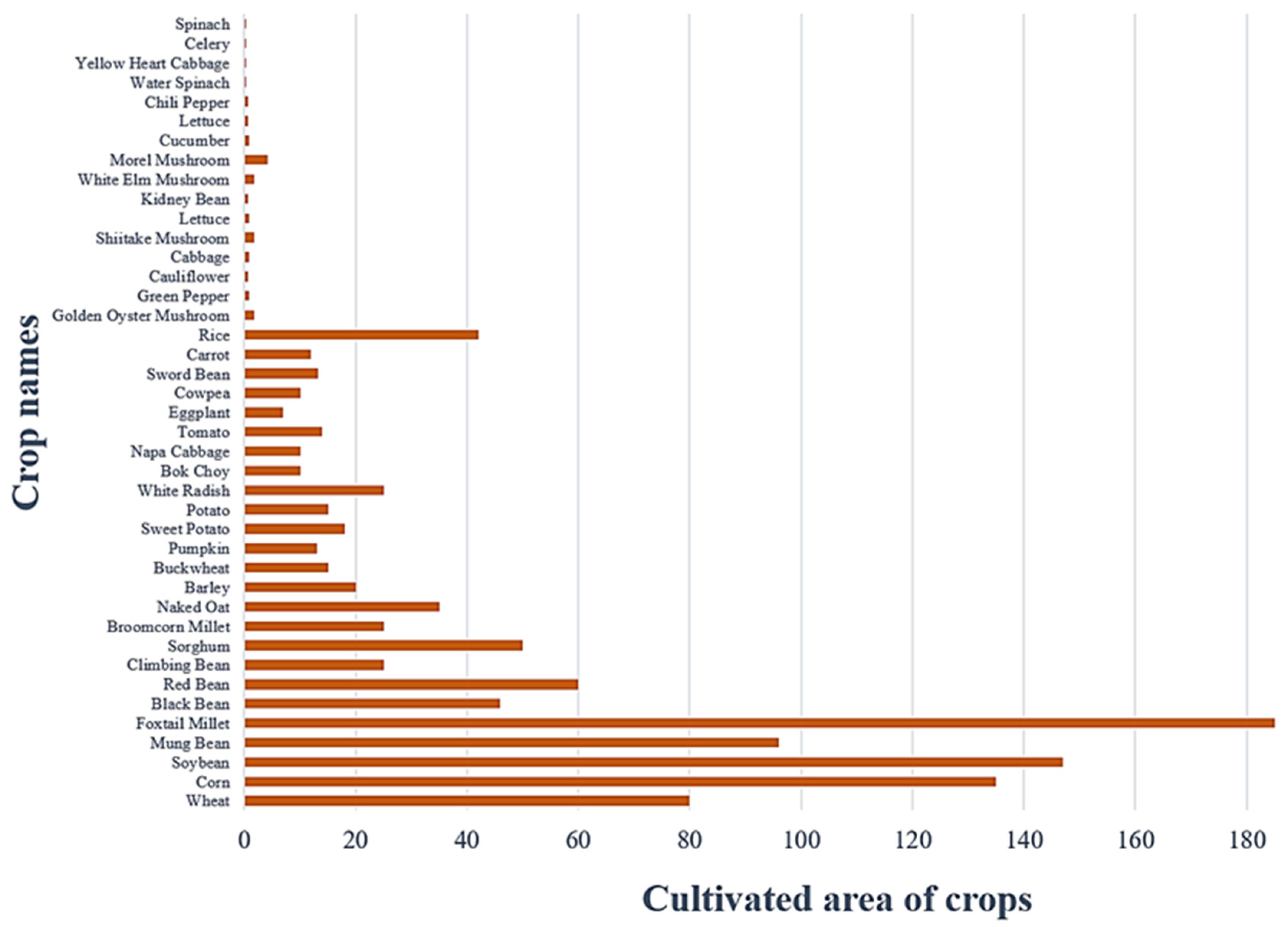
The largest cultivated area is allocated to grain crops, with millet occupying the largest portion and pumpkin the smallest. Subsequently, vegetable cultivation areas are described, where potatoes and white radishes have the largest cultivated areas, whereas lettuce, oilseed lettuce, water spinach, yellow heart cabbage, green peppers, tomatoes, cauliflower, cabbage, eggplant, cucumbers, small bok choy, celery, and spinach have the smallest areas, each covering only 0.05 acres. Lastly, the edible fungi cultivation area is outlined, with all four types of edible fungi having a cultivation area of 0.1 acres. The specific planting areas for each crop are illustrated in Figure 2.

2.1.4. Data on the Yields, Costs, and Prices in 2023

Overall, in terms of crop yield per acre, grain crops exhibit the highest productivity, followed by vegetable crops, with edible fungi yielding the least. Regarding planting costs, edible fungi generally incur higher expenses compared to vegetable crops, while grain crops remain the most cost effective. In terms of average unit selling price, edible fungi command the highest prices, whereas grain and vegetable crops are comparably priced. According to available data, weather conditions in North China during 2023 were largely favorable, promoting corn growth and maturation. Specifically, from July onward, abundant rainfall significantly alleviated drought conditions, thereby enhancing the growth of various crops. Based on these observations, no significant market surplus or supply shortages for agricultural products were identified in North China in 2023. Consequently, this study considers the 2023 crop yields as projected future sales volumes. The anticipated sales figures for selected crops are presented in Table 1.

2.2. Problems and Methods

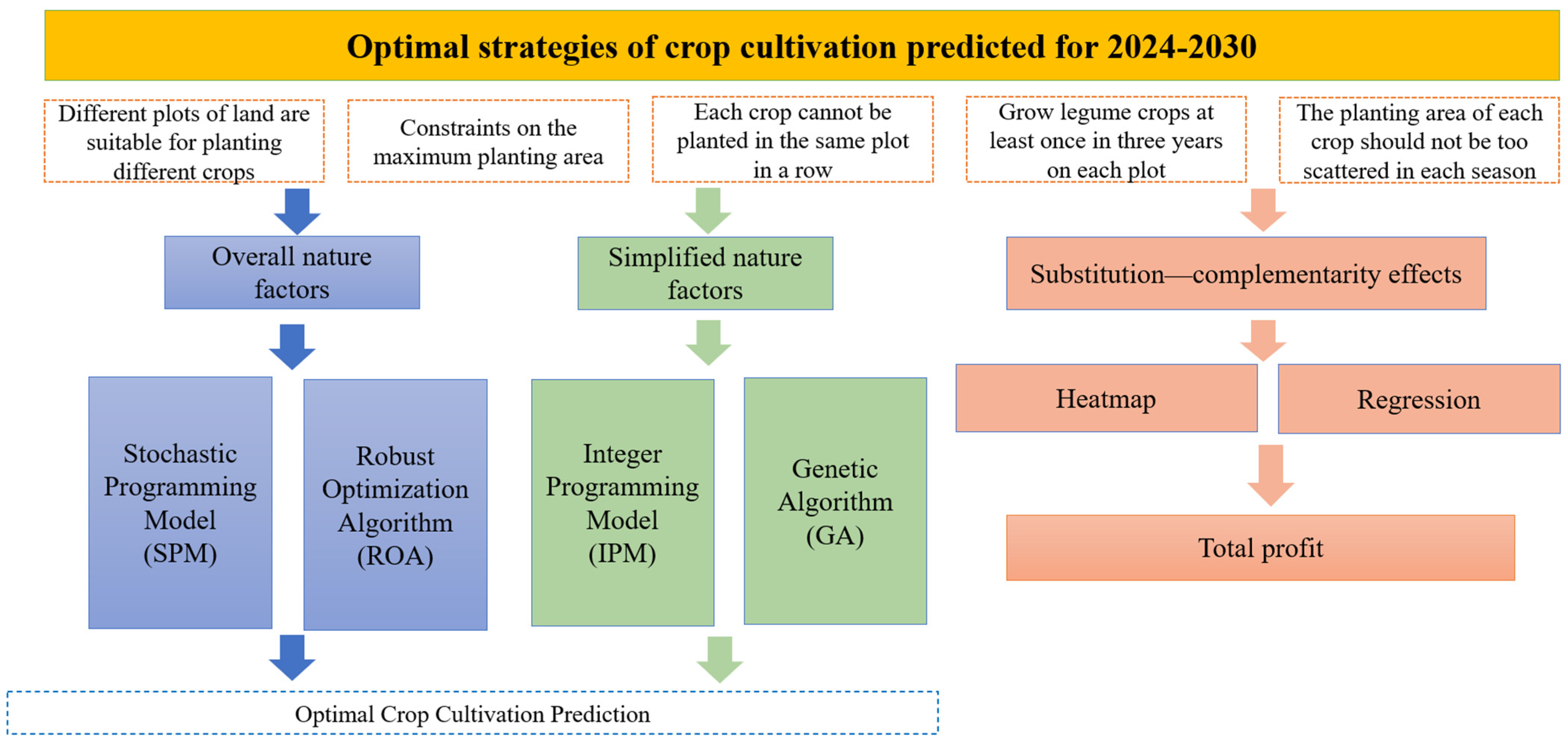
This study introduces an integrated framework for optimizing crop planting patterns that synergistically combines planning models with robust optimization algorithms (ROAs) and genetic algorithms (GAs) in Figure 3. The methodology addresses the problems of crop planting optimization through three interconnected components:
(1) Under primary constraints and accounting for uncertainties in crop sales volume, planting costs, yield per unit area, and selling prices, a stochastic programming model (SPM) is constructed. This model is solved using ROA to estimate total agricultural revenue for 2024–2030.
(2) With identical constraints and assuming all parameters (sales volume, costs, yield, prices) remain constant at 2023 levels, an integer programming model (IPM) is formulated. The solution is obtained via genetic algorithms, providing projected total crop cultivation revenue for 2024–2030.
(3) Under consistent constraints while comprehensively considering uncertainties and the substitutability–complementarity effects, relationships are visualized through heatmaps, and regression models are developed to generate optimized total profit projections for 2024–2030.
Figure 3. Workflow diagram: three interrelated components to solve the problem of crop cultivation optimization.
Agriculture 15 01736 g003

2.2.1. Optimized Planting Strategy with Overall Nature Factors

Wheat and corn sales grow 5–10% yearly; other crops vary slightly (±5%). Yields could shift ±10% due to weather. Planting costs rise ~5% annually. Grain prices stay stable, vegetables gain ~5% yearly, while fungi (especially truffles) drop 1–5% per year. Given these uncertainties, it is essential to develop an SPM optimization model incorporating multiple random variables to address the problem effectively.
By modeling fluctuating parameters such as per acre yield, sales price, expected sales volume, and planting costs as random variables, the objective function is defined to maximize the total revenue from 2024 to 2030. The key constraint conditions include the following: (1) different plots of land are suitable for specific crops; (2) limitations on the maximum planting area; (3) prohibition of consecutive planting of the same crop on the same plot (requiring crop rotation); (4) each plot must be planted with leguminous crops at least once every three years; and (5) the planting area for each crop in a single season should not be overly dispersed, and the planting area on any single plot should not be excessively small. A stochastic optimization model incorporating multiple random variables is established.

2.2.2. Optimized Planting Strategy with Restricted Natural Factors

Under the assumption that the expected sales volume, planting costs, per unit area yield, and sales price of various crops remain stable compared to 2023, the optimal planting plan for agricultural crops from 2024 to 2030 is to be determined under two distinct sales scenarios. In the first scenario, a portion of the produce remains unsold, leading to waste. In the second scenario, any excess production is sold at a discounted price equivalent to 50% of the 2023 sales price. Clearly, the objective is to maximize total revenue from 2024 to 2030 while satisfying all constraint conditions. The primary constraints are consistent with those outlined in Section 2.2.1, and the optimization process becomes significantly more complex under these conditions. A key challenge lies in formulating the constraint conditions and integrating them into the model as criteria for identifying the optimal solution. Even when considering only the constraint that leguminous plants must be grown at least once every three years, it is necessary to evaluate the optimal planting plan over a three-year cycle rather than focusing on a single year. Consequently, addressing multiple constraint conditions simultaneously presents a significant challenge. To tackle this issue, an integer programming model is constructed where decision variables represent the crop types planted on each plot during various seasons, and the objective function represents the total profit accumulated over a seven-year period. The main challenge of this model is the large number of variables, as each plot, season, and crop type requires a corresponding decision variable, resulting in tens of thousands of variables. To streamline the solution process, advanced heuristic algorithms such as genetic algorithms can be employed.

2.2.3. Correlation Analysis and Multi-Objective Optimization

In practical agricultural operations, different crops may exhibit certain substitutability and complementarity, which indicates the expected sales volume, sales price, and planting costs are interrelated. To formulate the optimal crop planting strategy for the period of 2024 to 2030, it is crucial to comprehensively consider these correlated factors. This requires the capability to construct a sophisticated optimization model that accounts for the interrelationships among various crops as well as the relationships among sales volume, price, and cost. Consequently, the following treatments have been conducted. Correlation analysis and multi-objective optimization models are employed to balance planting strategies across different crops, followed by data simulation and solution derivation. In analyzing these factors, two key aspects can be considered: (1) the substitutability and complementarity among crops—such as the potential for corn and wheat to serve as substitutes for each other under specific conditions; and (2) the interdependencies among sales volume, price, and cost—for example, whether an increase in sales volume may lead to changes in pricing or influence cost fluctuations. These relationships can be quantitatively assessed using techniques such as correlation coefficient matrices and regression analysis.

3. Models and Algorithms

3.1. Research Problem Overview

Based on the constraint of limited arable land resources in rural areas and adaptation to local conditions, this study focuses on developing the organic cultivation industry for sustainable development of the rural economy. To optimize field management, enhance production efficiency, and mitigate cultivation risks, we integrate a multi-model framework with optimization algorithms to generate a precise seven-year planting forecast. The specific objectives are as follows:
(1) Under multiple uncertainties across land, climate, and market factors, we employ SPM and ROA to both maximize profitability and design optimal cultivated strategies that balance profitability and robustness.
(2) Under simplified constraints, we combine IPM with GA to optimize crop cultivation for efficiency enhancement objectives, deriving optimal solutions for resource allocation and crop mix configuration.
(3) Considering the substitution–complementarity effects of crops, we synthesize correlation analysis (heatmaps) and regression modeling (linear/polynomial) to empirically optimize planting strategies. Model selection is determined by the strength of linear relationships via scatter plots, thereby enhancing agricultural outcomes.
The nomenclature mentioned in our models are summarized in Table 2.

3.2. Construction of the Crop Planning Prediction Model

3.2.1. Stochastic Programming Model (SPM)

Based on the aforementioned analysis, we take into account two primary factors that are climatic uncertainty and market fluctuation. Climatic uncertainty affects the expected sales volume of crops and the yield per acre, while market fluctuation affects the planting cost and sales price of crops.
The expected annual growth rate of crop sales volume, the annual change rate in yield per acre, the annual fluctuation in planting cost, and the annual change rate of sales price are modeled as random variables. The decision variable is defined as X t i j , representing the area allocated for planting the j-th type of crop on the i-th plot of land in the t-th year. SPM is constructed to establish the relationship between the decision variables and the total planting profit over seven years. The planning prediction that maximizes the total profit is identified as the optimal cropping strategy for the village from 2024 to 2030. In this study, it is assumed that both the annual growth rate of crop planting costs and the annual growth rate of vegetable crop sales are 5%.
For wheat and maize, the average annual growth rate of their projected future sales volumes is expected to range from 5% to 10%. The projected sales volume for year t (t > 2023) is given by
W 1 t j = W 1 t j ( 1 + ω 1 ) t 2023         j = 6,7  
Here, W 1 t j represents the projected sales volume (equivalent to production volume) of wheat and maize in 2023, and ω 1   denotes the average annual growth rate of their future projected sales volumes.
For other crops, the projected annual sales volumes relative to 2023 levels fluctuate within a range of −5% to 5%. The projected sales volume for year t (t > 2023) of these crops is given by
W 2 t j = W 2 t j ( 1 + ω 2 ) t 2023 j = 1 , 2 , , 41
Here, W 2 t j   denotes the projected sales volume (equivalent to production volume) of other crops excluding wheat and maize in 2023, and ω 2   represents the average annual fluctuation rate of their future projected sales volumes.
The annual fluctuation rate of crop yield per acre ranges from −10% to 10%. Therefore, the yield per acre for crops in year t (t > 2023) is given by
L j = L j ( 1 + l ) t 2023   j = 1 , 2 , , 41
Here, L j   represents the yield of each crop in 2023, and l denotes the annual variation rate of the yield per mu for crops.
Under the influence of market conditions, the annual growth rate of cultivation costs for each crop fluctuates around 5%. Therefore, the cultivation cost for crops in year t (t > 2023) is given by
W 2 t j = W 2 t j ( 1 + ω 2 ) t 2023 j = 1 , 2 , , 41 ,
Here, C j   denotes the cultivation cost of crops in 2023.
Under the influence of market economy dynamics, the sales price of vegetable crops increases annually, with a growth rate fluctuating around 5%. The sales price for vegetable crops in year t (t > 2023) is given by
Q 1 j = Q 1 j ( 1 + 5 % ) t 2023 j = 1 , 2 , , 41
Here, Q 1 j   denotes the sales price of vegetable crops in 2023.
Under the influence of the market economy, the sales prices of edible fungi crops exhibit a stable yet declining trend, with an annual decrease of approximately 1% to 5%. Notably, the sales price of morel mushrooms declines by 5% annually. Therefore, the sales price of edible fungi crops in year t (t > 2023) is given by
Q 2 j = Q 2 j ( 1 + q 2 ) t 2023 + Q 241 ( 1 + 5 % ) t 2023 j = 1 , 2 , 3 , , 41
Here, Q 2 j   denotes the sales price of edible fungi crops in 2023, and q 2 represents the annual decline rate for edible fungi.
The annual yield of planted crops is given by
P t i j = X t i j L j
The annual cultivation cost of planted crops is given by
Y t i j = X t i j C j
Total profit is given by
Z = i = 1 54 j = 1 41 P t i j ( Q 3 j + Q 1 j + Q 2 j ) i = 1 54 j = 1 41 Y t i j
Here, Q 3 j   denotes the sales price of grain crops.
For the scenario where crop production exceeds projected sales volumes, resulting in oversupply, the total profit for the seven-year period from 2024 to 2030 is calculated as follows.
If yield does not exceed projected sales volume, the total profit is denoted as
m a x Z = t = 1 7 i = 1 54 j = 1 41 P t i j Q 3 j + Q 1 j + Q 2 j t = 1 7 i = 1 54 j = 1 41 Y t i j
If yield exceeds projected sales volume, the total profit is denoted as
m a x Z = t = 1 7 i = 1 54 j = 1 41 ( W 1 t j + W 2 t j ) Q 3 j + Q 1 j + Q 2 j t = 1 7 i = 1 54 j = 1 41 Y t i j
For the scenario where crop production exceeds projected sales volume, leading to discounted sales, the total profit for the seven-year period from 2024 to 2030 is calculated as follows.
If yield does not exceed projected sales volume, the total profit is denoted as
m a x Z = t = 1 7 i = 1 54 j = 1 41 P t i j Q 3 j + Q 1 j + Q 2 j t = 1 7 i = 1 54 j = 1 41 Y t i j
When the actual yield exceeds the projected sales volume, the total profit is calculated according to the rule that the portion of the output up to the projected sales volume is sold at the regular price, while any excess quantity is sold at half that price. The total profit is therefore the sum of the profits generated from these two segments.
Excess production is
P = m i n ( t = 1 7 i = 1 54 j = 1 41 P t i j W j )
Revenue from excess production is
Z = m i n ( t = 1 7 i = 1 54 j = 1 41 P t i j W j ) Q j 2
The maximum total profit is
m a x Z = W j Q j + Z t = 1 7 i = 1 54 j = 1 41 Y t i j
The constraints of SPM are discussed as follows.
Since the total area of each land plot is fixed, the sum of cultivation areas allocated to crops on any plot cannot exceed its fixed total area, i.e.,
j = 1 41 X i j S i ,    i = 1 , 2 , , 54 ,
where S i represents the maximum cultivation area of the i-th land plot.
1.
To mitigate yield reduction caused by consecutive planting of the same crop on the same plot, i.e., continuous cropping, the following constraint is enforced as
X t i j X t + 1 i j = 0 .
2.
To leverage the soil-enriching benefits of legume root nodules (rhizobia) for subsequent crops, the constraint is imposed starting from 2023 that each land plot must cultivate legumes at least once within any consecutive three-year period and is denoted as
t = 1 3 x t i j > 0 .
3.
To ensure rational land utilization and avoid undersized cultivation, we assume that the total cultivation area allocated to crops on any land plot is deemed reasonable if and only if the sum of planted areas exceeds half of the plot’s fixed total area. The constraint is denoted as
j = 1 41 X i j S i 2 .
4.
Due to variations in land plot types and seasonal conditions, the variety of crops that can be cultivated on each plot is restricted. It necessitates the constraint that is denoted as
X i j r i j S i ,   r i j { 0 ,   1 }
Here, r i j is an indication function that indicates whether the i -th piece of land is suitable for planting the j -th type of crop, with 1 representing suitability and 0 representing unsuitability.
Overall, the identified constraints can be summarized as follows.
S t .     j = 1 X i j S i j X t i j X t + 1 i j = 0 t = 1 3 x t i j > 0 j = 1 41 X i j S i 2 X i j r i j S i X i j 0 , P i j 0

3.2.2. Integer Programming Models (IPMs)

We further simplify the above model by predicting the maximum sales profit and the optimal planting strategy under a more ideal scenario. Specifically, we assume that the expected sales volume, planting cost, yield per acre, and sales price of various crops remain relatively stable compared to 2023. In addition, if the total yield of each crop per season exceeds the expected sales volume, the excess cannot be sold at normal prices. The decision variable is still defined as X i j , representing the area of the j-th crop planted on the i -th plot of land. The planting plan that maximizes annual profit Z is identified as the optimal planting plan for each year, and an IPM linking the decision variable to profit is subsequently established. The annual yield of crops planted is represented as
P i j = X X i j · L j
P i j is the total yield of the j -th crop planted in the   i -th plot, X i j is the area of the i -th plot allocated to the j -th crop, L j is yield per unit area of the j -th crop. Hence, the total yield denoted as i = 1 54 j = 1 41 P i j .
The annual cultivation cost is represented as
Y i j = X i j · C j
Y i j is the total cultivation cost for planting the j -th crop in the i -th plot, X i j is the area of the i -th plot allocated to the j -th crop, C j is the cultivation cost per unit area for the j -th crop. Hence, the total cultivation cost is denoted as i = 1 54 j = 1 41 Y i j .
The total profit is calculated by
Z = i = 1 54 j = 1 41 P i j Q j i = 1 54 j = 1 41 Y i j
Crop prices generally exhibit a “bimodal cyclical fluctuation” pattern, oscillating around a central value [34,35]. Therefore, we adopt the average value of each crop’s 2023 price range as its sales unit price. To account for unsold excess production, the total profit over the seven-year period from 2024 to 2030 is calculated as follows.
If yield does not exceed projected sales volume, the total profit is
m a x Z = t = 1 7 i = 1 54 j = 1 41 P t i j Q j t = 1 7 i = 1 54 j = 1 41 Y t i j
If yield exceeds projected sales volume, the total profit is
m a x Z = W j Q j t = 1 7 i = 1 54 j = 1 41 Y t i j
In the scenario where the surplus crops are sold at discounted prices, the total profit from 2024 to 2030 is calculated as follows.
If yield does not exceed projected sales volume, the total profit is
m a x Z = t = 1 7 i = 1 54 j = 1 41 P t i j Q j t = 1 7 i = 1 54 j = 1 41 Y t i j
When actual yield exceeds projected sales volume, total profit is calculated according to the rule that the portion of output up to the projected sales volume is sold at the regular price, while any excess quantity is sold at half that price. The total profit is the sum of the profits generated from these two segments.
Excess production is
P = m i n t = 1 7 i = 1 54 j = 1 41 [ P t i j ( W 1 t j + W 2 t j ) ]
Excess profit is
Z = m i n t = 1 7 i = 1 54 j = 1 41 [ P t i j ( W 1 t j + W 2 t j ) ] Q i j + Q i j + Q i j 2
If yield exceeds projected sales volume, the total profit is
m a x Z = t = 1 7 i = 1 54 j = 1 41 W i j + W i j Q i j + Q i j + Q i j + Z t = 1 7 i = 1 54 j = 1 41 Y t i j
The objective function is calculated as follows in two scenarios.
  • Scenario A: The crop surplus will be unsold, resulting in waste.
If yield does not exceed expected sales volume, the total profit is
m a x Z = t = 1 7 i = 1 54 j = 1 41 P t i j Q j t = 1 7 i = 1 54 j = 1 41 Y t i j
If yield exceeds expected sales volume, the total profit is
m a x Z = t = 1 7 W t j Q j t = 1 7 i = 1 54 j = 1 41 Y t i j
  • Scenario B: The crop surplus is sold at a 50% discount of the selling price.
If yield does not exceed expected sales volume, the total profit is
m a x Z = t = 1 7 i = 1 54 j = 1 41 P t i j Q j t = 1 7 i = 1 54 j = 1 41 Y t i j
If yield exceeds expected sales volume, the total profit is
m a x Z = t = 1 7 W t j Q j + m i n t = 1 7 i = 1 54 j = 1 41 P t i j W j Q j 2 t = 1 7 i = 1 54 j = 1 41 Y t i j
The constraints of SPM are modeled as the same as the ones of the IPM in mathematics.

3.3. Algorithms

3.3.1. Hybrid Stochastic–Robust Optimization Algorithm

A robust optimization algorithm (ROA) is an advanced optimization methodology specifically designed to address parametric uncertainty. Its central concept involves handling uncertain parameters within the objective function and constraints, whose true values remain unknown at the time of decision-making. To manage the uncertainty, a deterministic uncertainty set is predefined, which encompasses all possible or relevant values of these parameters. The primary goal of robust optimization is to identify a solution, referred to as a robust feasible solution, within a given basic feasible region. This solution must remain feasible for all potential realizations of uncertainty while optimizing the objective function value under the worst-case realization of uncertainty. A notable feature of this approach is the distributional robustness, as it does not require knowledge of the probability distribution of the uncertain parameters. However, the level of conservatism in the resulting solution is heavily influenced by the size and structure of the predefined uncertainty set, necessitating a careful balance between robustness and average performance. ROA has been proven particularly advantageous in critical applications where precise probability distribution information is unavailable or where the tolerance for system failure is exceptionally low [36,37].
Furthermore, we analyze the effectiveness of ROA by comparing it with alternative methods such as Fuzzy Optimization (FO) and Bayesian Analysis (BA). FO faces challenges in quantifying extreme risks and exhibits low computational efficiency, especially for nonlinear problems. However, the study area—a rural mountainous region in North China—is highly prone to extreme events. BA performs well in environments with high-frequency data, such as continuous market price monitoring, but it is heavily dependent on accurate prior distributions and high-quality data. Moreover, BA can encounter computational difficulties, such as Markov Chain Monte Carlo (MCMC) convergence issues. In contrast, the ROA aims to identify feasible solutions that remain effective in the worst-case scenarios by characterizing parameter uncertainties through an uncertainty set. The ROA does not require assumptions regarding data distributions, making it particularly suitable for small-sample or data-scarce situations. Additionally, the ROA has proven highly effective in managing risks associated with extreme climate and price volatility [38], and its computational complexity is manageable and practical for real-world implementation. Therefore, we adopt the ROA in our paper.
Given that the aforementioned model involves numerous fluctuating variables, we assume that all parameter variations follow a normal distribution. To ensure computational simplicity and clarity, the types of these stochastic variables are categorized into three distinct categories including robust fluctuation variation, normal fluctuation variation, and the worst-case fluctuation variation.
  • Robust Fluctuation Variation: The parameters are set to maximize positive impacts on total profit as follows: (a) Projected Sales Volumes: Wheat and maize maintain a high annual growth rate of 10%. Other crops sustain a growth rate of 5%. (b) Yield per Acre: Annual yield increases by 10% for all crops. (c) Cultivation Costs: Annual cost growth averages 5%, but under robust fluctuation, the rate is set to the lower bound of its fluctuation range around 3%. (d) Market Prices: The sales prices of grain crops fluctuate within −2% to 2% and increase by 2% annually. The sales prices of vegetable crops fluctuate in the range from 3% to 7% with 7% annual growth. The sales prices of edible fungi decline by 1% annually, with only morel mushrooms experiencing a 3% annual decrease.
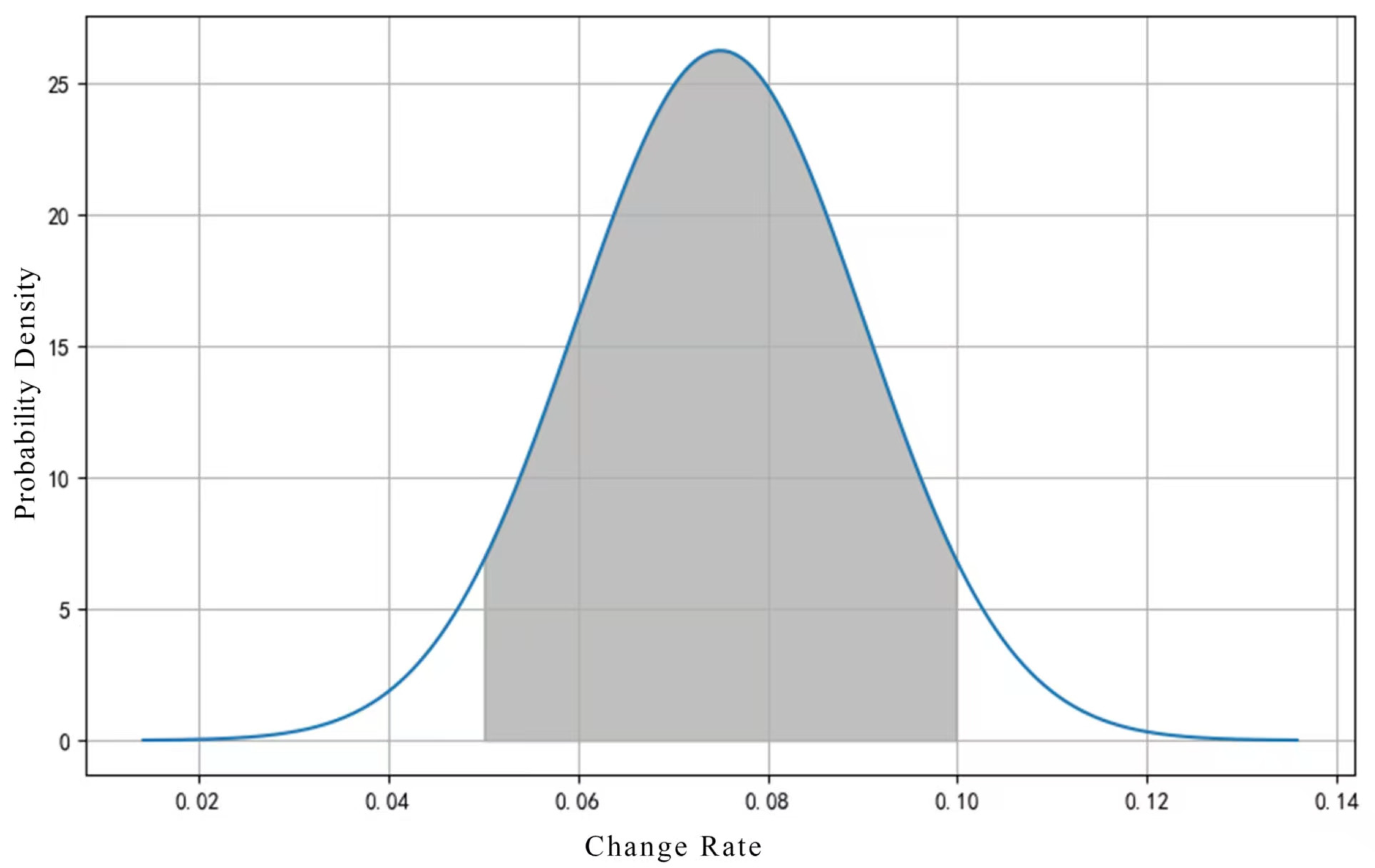
  • Normal Fluctuation Variation: It is assumed that all parameter fluctuations adhere to a normal distribution. For instance, the statistical distribution of the annual change rate in the expected sales volume of wheat and corn is illustrated in Figure 4. The grey block indicates that the most likely range for the anticipated annual growth rate of sales volume for wheat and corn is between 5% and 10%.
Therefore, in the normal fluctuation scenario, the anticipated annual growth rate of sales volume for wheat and corn is 7.5%. The annual increase in planting costs is projected to be 5%. The selling price of grains is expected to remain stable, while the selling price of vegetable crops is forecasted to rise by 5% annually. Conversely, the selling price of edible fungi is anticipated to decrease by 3% annually, and the selling price of morel mushrooms is expected to decline by 5% annually.
  • The Worst-Case Fluctuation Variation: the expected annual growth rate of sales volume for wheat and corn is 5%, whereas the sales volume of other crops decreases by 5% annually. Additionally, the crop yield per acre decreases by 10% annually, while the planting cost of crops increases by 7% annually. Furthermore, the selling price of edible fungi is estimated to decrease by 5% each year, with the price of morel mushrooms declining by 7% annually.
In summary, the results are synthesized in Table 3.
Robust optimization is a mathematical optimization method for decision-making under uncertainty. The core idea lies in constructing an uncertainty set to describe parameter perturbations and optimizing crop planting schemes under various interfering factors, thereby ensuring that agricultural profits remain at a relatively high level even under adverse conditions. This optimization algorithm is particularly suitable for scenarios where data distributions are difficult to model accurately.
The proposed algorithm is illustrated in Algorithm 1.
Algorithm 1 Proposed ROA to Solve (9) in SPM
1: Initialization :   Initialize   decision   variables   { X t i j ( 0 ) }   .   Define   the   distribution   of   random   variables   { ω 1 , ω 2 , l , q 2 } , iteration index i = 0, and convergence accuracy ϵ.
2: repeat
3: Set i = i + 1.
4: Generate   random   samples   { ω 1 ( i ) , ω 2 ( i ) , l ( i ) , q 2 ( i ) }   and   update   { W 1 t j i , W 2 t j i , L j i , Q 1 j i , Q 2 j i }.
5: To solve (6):
If   { P t i j ( i ) W t j ( i ) } ,   calculate   { Z ( i ) }   according   to   ( 10 ) .   Else ,   calculate   { Z ( i ) } according to (13).
6: Calculate   m a x Z ( i ) under (16).
7: until convergence.
8: Output :   X t i j *   and   Z * .

3.3.2. Hybrid Integer-Programming–Genetic-Optimization Algorithm

Due to the large number of variables involved in the IPM, as well as the complex constraints and nonlinear objective function, we consider using the genetic algorithm (GA) [39] for computation. GA is a heuristic search algorithm that simulates the mechanisms of natural selection and genetics, which is used to solve optimization problems. The solution process of the GA for this problem is as follows:
(a) First, we represent the planting plan for each plot of land as a gene, and the overall planting plan as an individual. The total profit (i.e., the objective function) is used as the fitness function.
(b) Initial population generation: use the planting plan from 2023 as the initial solution.
(c) Fitness evaluation: calculate the total profit for different planting plans.
(d) Choose individuals with higher fitness values (i.e., planting plans) from the population to enter the next generation.
(e) Randomly select crossover points on the chromosomes, exchange the parts between the crossover points to generate new individuals; randomly select a gene on the chromosome and make a minor change to it. This generates new individuals, increases the diversity of the population, and continues the search for the optimal solution.
(f) The process is terminated when the specified number of iterations is reached, or the fitness value is sufficiently high.
In the selection process, the probability of each individual being selected can be expressed by the following formula:
q i = f i i = 1 N f i
Here, q i represents the probability of the i -th individual being selected; f i is the fitness value of the i -th individual, which corresponds to the total profit; N is the population size, which is the total number of plans. The formula ensures that individuals with higher fitness values have a higher probability of being selected for the next generation.
In the crossover process, two planting plans are crossed to produce a new planting plan. Let the probability of crossover be p j i a o c h a . The formula for generating a new planting plan through crossover is denoted as
M = p j i a o c h a D + ( 1 p j i a o c h a ) B
The GA is specifically summarized in Algorithm 2.
Algorithm 2 Proposed Genetic Algorithm (GA) to Solve (19)
1: Generate   initial   population   of   solutions   { X i j ( k ) , k = 1 . . K } , Set GA parameters: population size K, max generations G.
2: repeat
3: Set i = i + 1.
4: For   each   solution   { X i j ( k ) } , calculate yield and costs according to (17) and (18), respectively.
5: if   { P i j W j } ,   calculate   { Z ( k ) } according to (20).
Else ,   calculate   { Z ( k ) } according to (25).
6: Randomly   adjust   { X i j }   values   while   maintaining :   { X t i j X t + 1 , i j = 0 }   and   { t = 1 3 x t i j > 0 } .
7: For   top   10 %   { Z * } , solve IP subproblem. Compute (25) under (14).
8: until Convergence.
9: Output :   Best   solution   { X i j * }   and   profit   { Z * } .

4. Results

4.1. Optimal Crop Planting Results with Multi-Factor Constraints

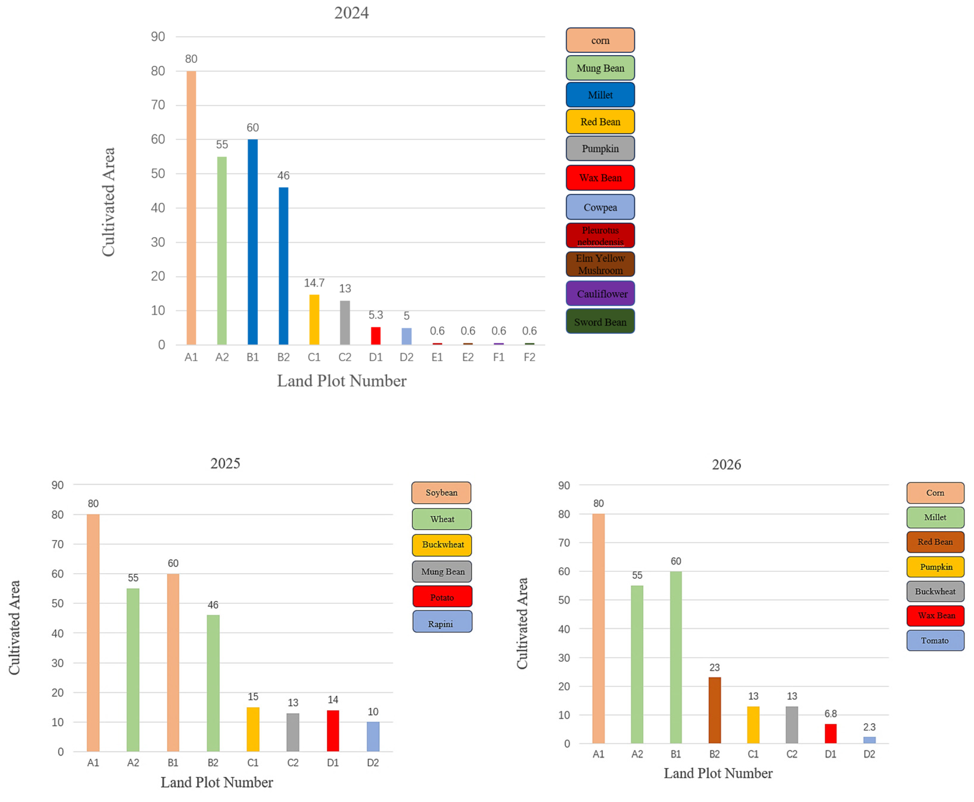
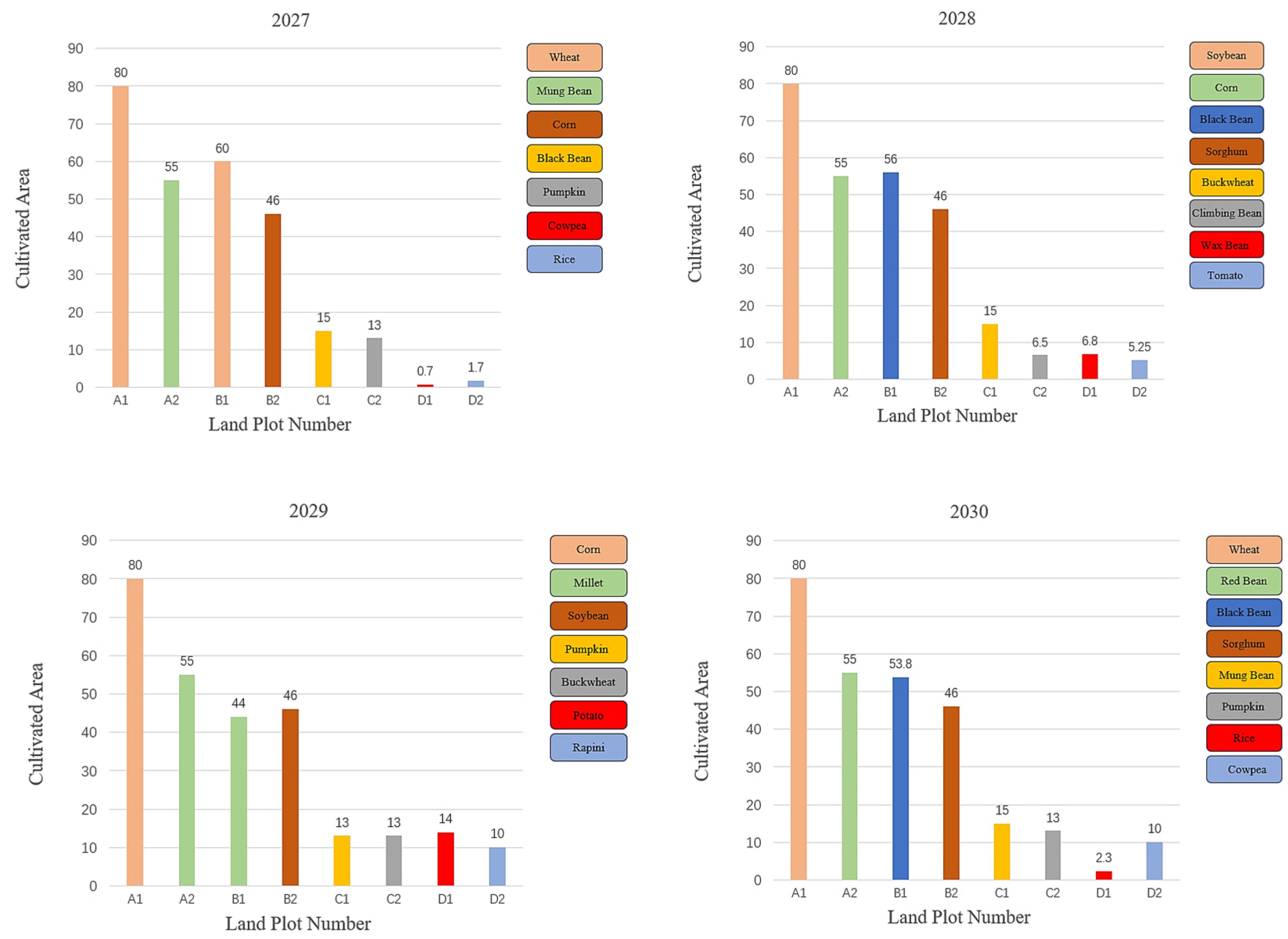
Based on the above SPM with the ROA as the solution, we get the results how the crops are planted elaborately for total profit maximization. Partial results of the optimized planting strategy are shown in Table 4 and Table 5 and seven-year planting plans of typical crops from 2024 to 2030 are depicted in Figure 5. We can further calculate the total profits in three different fluctuation scenarios. In the robust fluctuation scenario, the total profit is 53.491 million yuan. In the normal fluctuation scenario (the most likely scenario), the total profit is 45.746 million yuan. In the worst-case fluctuation scenario, the total profit is 38.154 million yuan. It can be seen from the above that the harvest of crops will be significantly affected when encountering poor conditions. The profit under robust optimization shows a 16.93% increase (7.745-million-yuan absolute growth) compared to the normal fluctuation scenario.
To more intuitively present partial results of the planting plan, we have used a bar chart for representation. It is worth noting that if two plots have the same color, it means they are planted with the same crop.
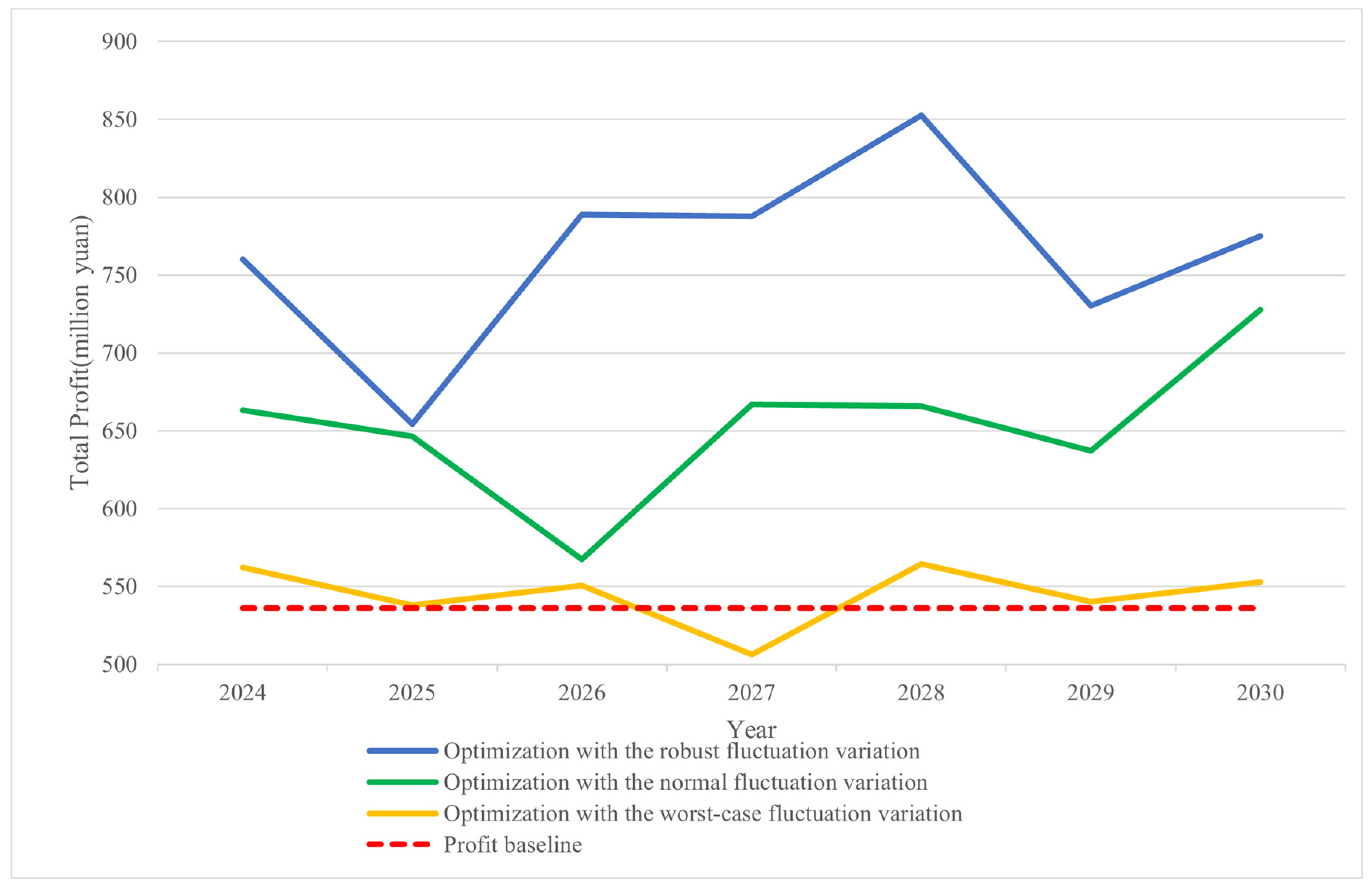
In Figure 6, the red dashed line represents the profit benchmark derived from historical rural income data. The blue solid line illustrates the optimized best-case scenario with the robust fluctuation variation, the green solid line depicts the optimized most probable scenario (i.e., the most likely outcome), and the yellow solid line shows the optimized worst-case scenario. The best-case and worst-case scenarios are considered extreme and rarely appear, corresponding to the maximum and minimum profit projections, respectively. In contrast, the optimized probable scenario is more commonly observed and robust, with results indicating that its profit performance consistently exceeds the established baseline.

4.2. Optimal Crop Planting Results with Restricted Constraints

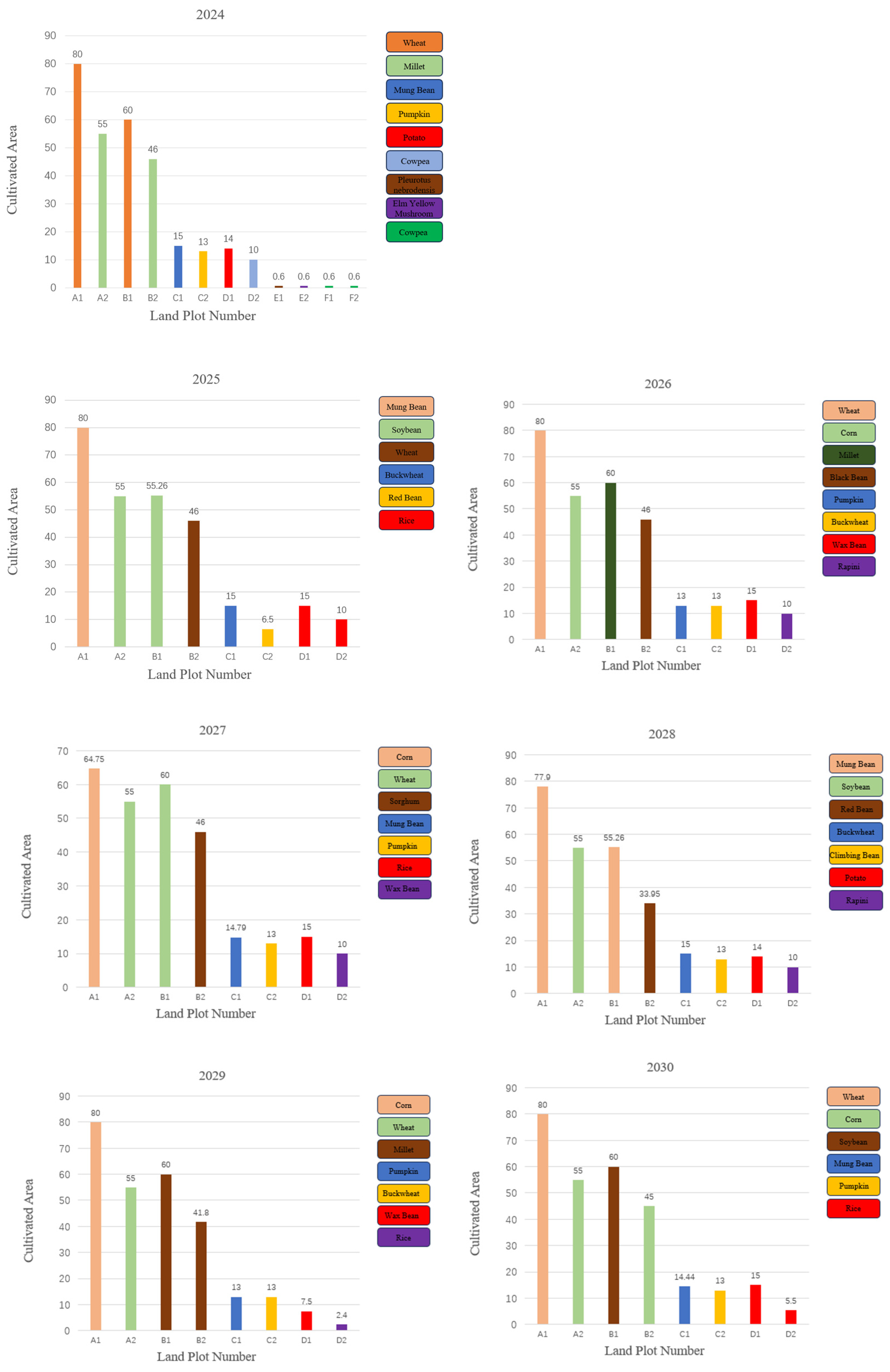
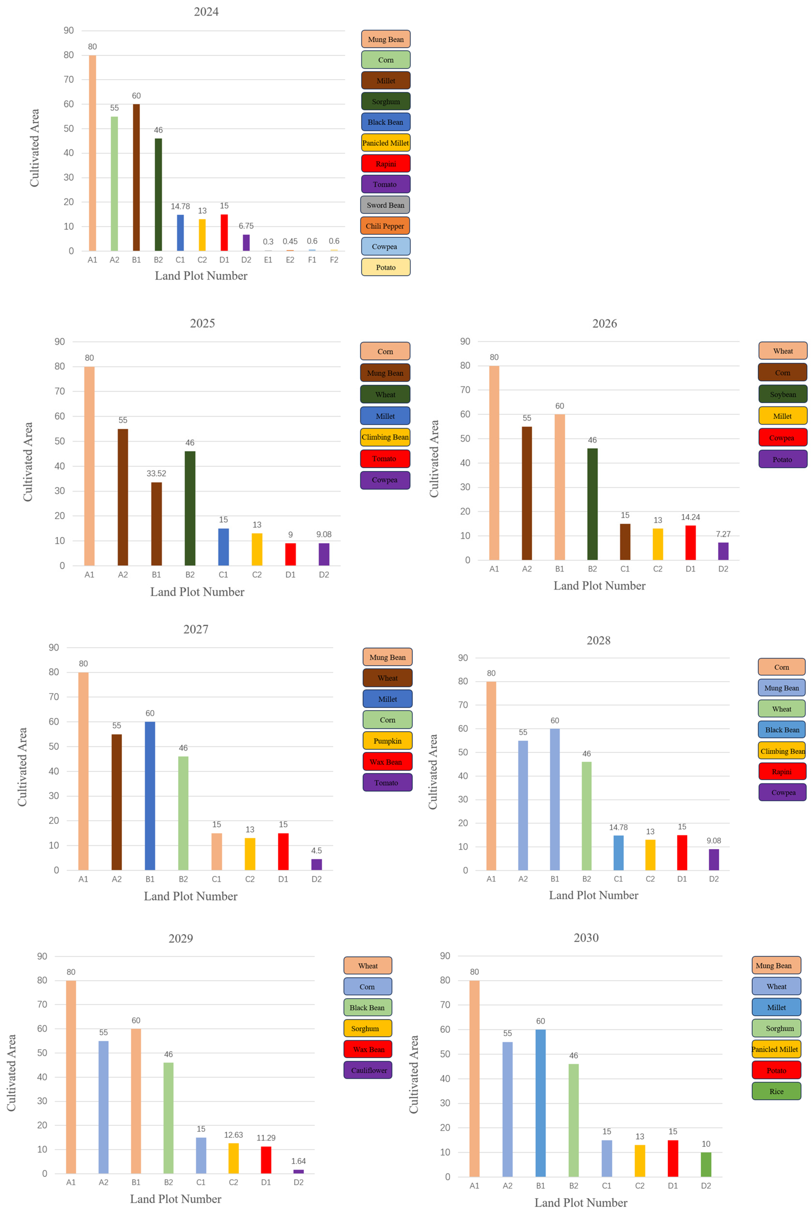
Based on the above IPM with GA as the solution, we obtain the results for how the crops are planted elaborately for total profit maximization. Partial results of the optimized planting strategy are shown in Table 6 and Table 7 (Scenario A) and in Table 8 and Table 9 (Scenario B), and seven-year planting plans of typical crops from 2024 to 2030 are depicted in Figure 7 (Scenario A) and Figure 8 (Scenario B).
The final calculation yields the total profit for the years 2024 to 2030 in two different scenarios (A and B):
(a) The total revenue when there is a surplus that cannot be sold is 42.6873 million yuan.
(b) The total revenue when the surplus part is sold at 50% of the original price is 46.586 million yuan.
It is evident that the revenue in the second scenario is higher than that in the first one. The results indicate that even though the excess part is sold at a 50% discount, it is still possible to achieve profitability by selecting crops with higher economic value for planting, thereby increasing the total revenue.
To conclude, we have identified the key parameters of two methods in all cases.
In Table 10, the SPM with ROA method achieves the highest profit growth rate of 42.5% in the optimal scenario and 21.8% in the normal scenario. In contrast, the profit growth rate declines to only 2.6% in the worst scenario. The IPM with GA method demonstrates profit growth rates of 13.7% and 24.1% in the scenarios A and B, respectively.
In addition, we set the land utilization rate in the optimal scenario as the benchmark at 100% and give the results in the other scenarios. We also use the optimized profit in the worst scenario as the baseline and compare it with the profits in the other scenarios to calculate the risk mitigation indicator. Compared to the profit baseline, both methods demonstrate varying degrees of profit improvement after optimization. In the method of the SPM with ROA, the optimal and the worst scenarios correspond to low-probability agricultural events, with the majority of events expected to cluster around the normal scenario. The IPM with GA method also shows notable performance advantages in certain specific scenarios.

4.3. Sensitivity Analysis

The key parameters including expected sales volume, yield per acre, planting cost, and selling price with their fluctuation ranges are shown in Table 11.
To evaluate the impact of these parameters on total profit, we conduct a single-factor sensitivity analysis, in which each parameter is varied individually while all other parameters are held constant at their baseline values (i.e., normal fluctuations). The results of percentage change in total profit are recorded in Table 12. The baseline scenario parameters are as follows.
Sensitivity analysis reveals that the annual growth rate of expected sales volume for wheat and corn is the most sensitive parameter whose sensitivity elasticity coefficient is the highest (6.8). Therefore, market trends should be monitored closely, and accurate forecast should be prioritized when considering crop planting strategies. Also, long-term sales contracts can be utilized to lock in volumes and mitigate profit volatility. Furthermore, the annual change rates of yield per acre (1.2), planting cost (2.6), and the annual growth rate of vegetable crops (2.6) exhibit moderate sensitivity. Hence, introducing drought-resistant crop varieties or adopting greenhouse cultivation methods can help reduce yield and cost fluctuations. The annual change rate of expected sales volume for other crops (1.04) and the annual price decline rate of edible mushrooms (−2.6) are relatively less sensitive. However, adjusting the mushroom planting ratio dynamically can still effectively hedge against price decline risks. Additionally, we recommend that the government establish targeted subsidies to encourage farmers in the mountainous regions of North China to cultivate cold-resistant wheat and water-saving corn. Concurrently, technical training programs should be implemented to support the adoption of these new crop varieties, ensuring their successful cultivation. This integrated approach aims to enhance both crop yields and farmers’ income (Table 13).

5. Discussion

5.1. Correlation Analysis with Heatmap

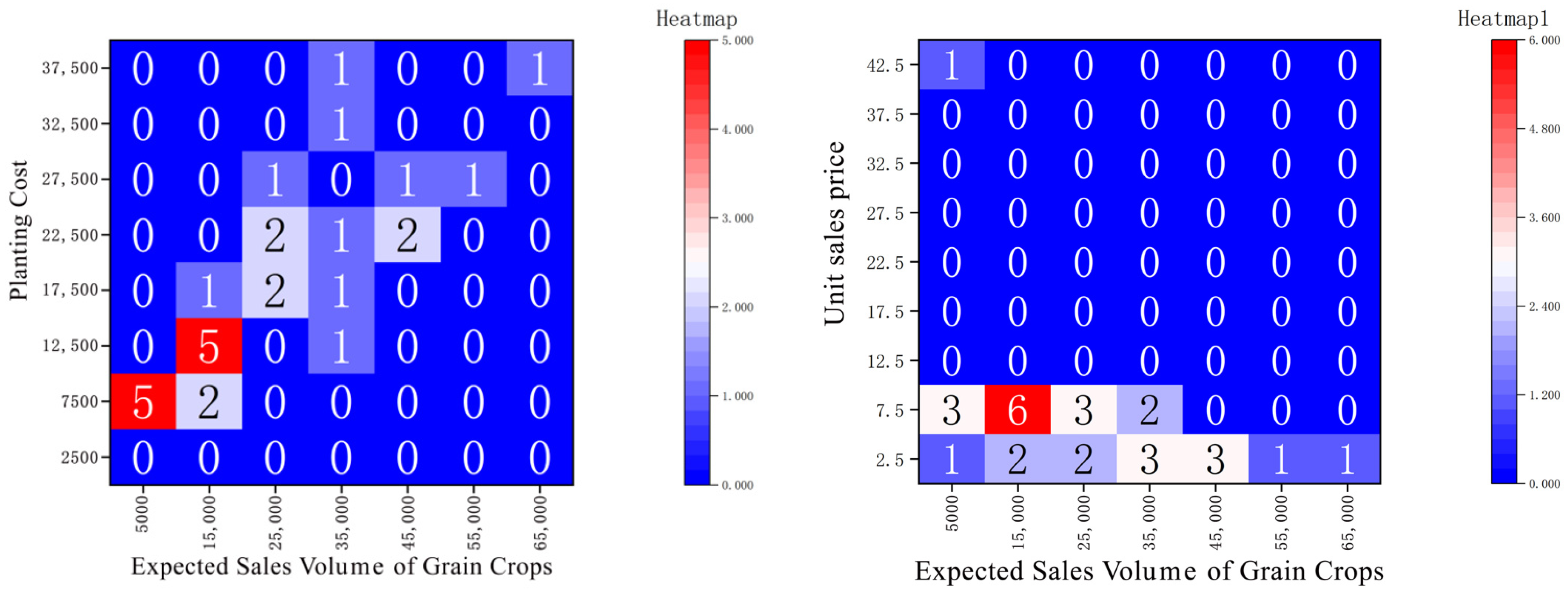
This study also takes into account the complementarity–substitutability effects between different crops that grain crops and edible fungi crops are substitutes for each other, and starchy vegetable crops are substitutes for grain crops such as wheat and rice. Meanwhile, grain crops are complementary to both vegetable crops and edible fungi crops. Accordingly, we explore the correlation between the expected sales volume, sales price, and planting cost of different types of crops. Using the data obtained in 2023, we create heatmaps of the expected sales volume of grain crops versus their planting cost and unit sales price, as shown in Figure 9. The heatmaps show that the expected sales volume of grain crops has a strong correlation with their planting costs, while the correlation with their unit sales prices is relatively weak.
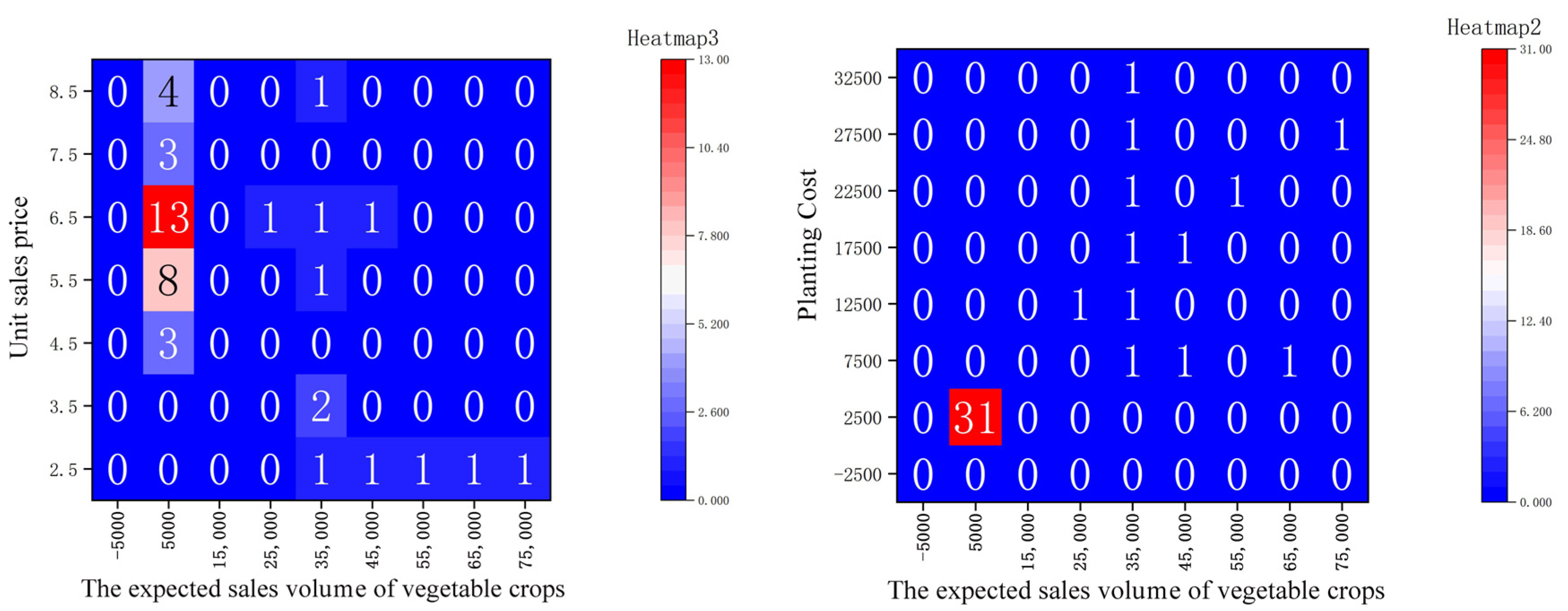
The correlation heatmap between the projected sales volumes of vegetable crops and their cultivation costs and unit selling prices is shown in Figure 10. The heatmaps indicate that the expected sales volume of vegetable crops has a weak correlation with their planting costs, while it has a strong correlation with their unit sales prices.
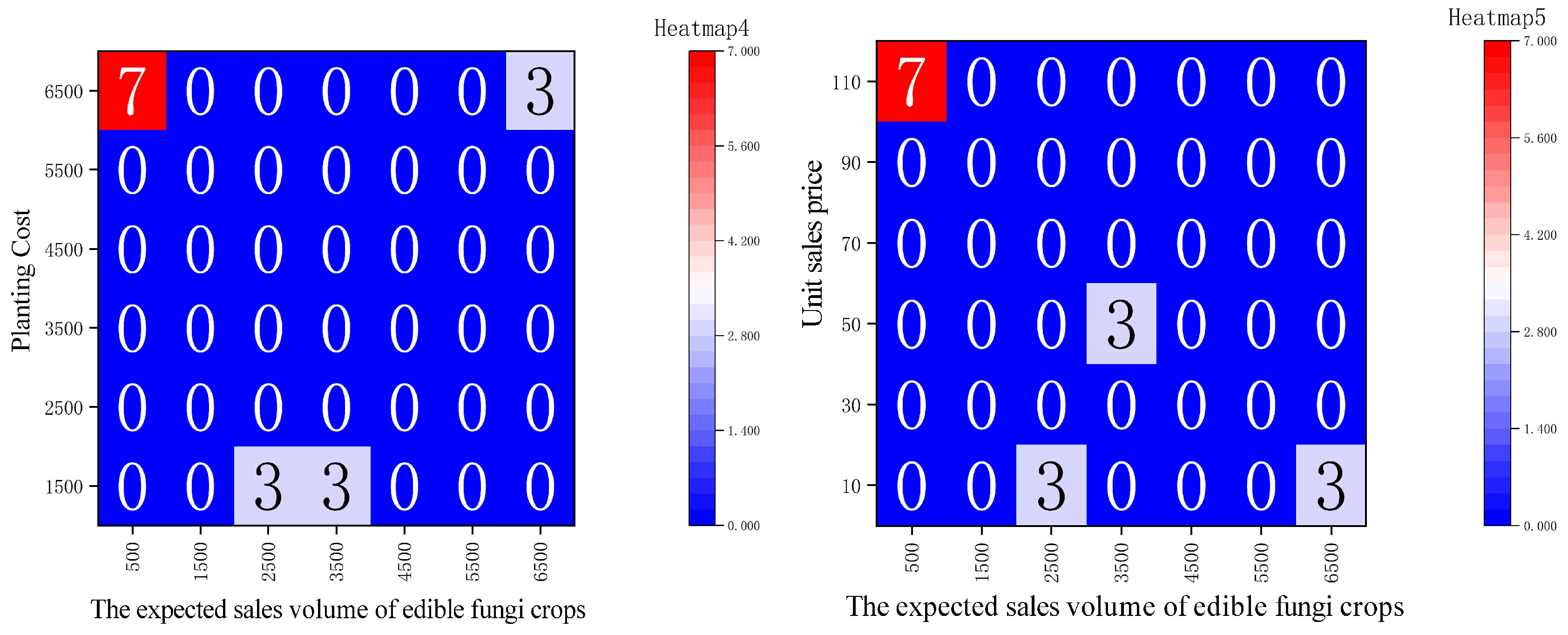
The heatmaps of the expected sales volume of edible fungi crops versus their planting costs and unit sales prices are shown in Figure 11. The heatmaps show that the expected sales volume of edible fungi crops has a similar and relatively weak correlation with both their planting costs and unit sales prices.
The complementarity–substitution effects among common crops are illustrated in Table 14. Varying degrees of substitutability exist among different crops—a characteristic influenced by factors such as yield potential, nutritional composition, and production requirements. The magnitude of the substitution coefficient reflects the strength of this relationship; for example, a coefficient of 0.95 for spinach, lettuce, and bok choy indicates a high degree of substitutability in their cultivation. The dynamics of crop substitutability and complementarity are determined not only by inherent biological characteristics but also by prevailing production conditions and market demand. As a result, this information serves as a crucial reference for agricultural practitioners, assisting them in making informed crop selection decisions that align with specific environmental and economic conditions, thereby enhancing agricultural profitability.

5.2. Regression Analysis

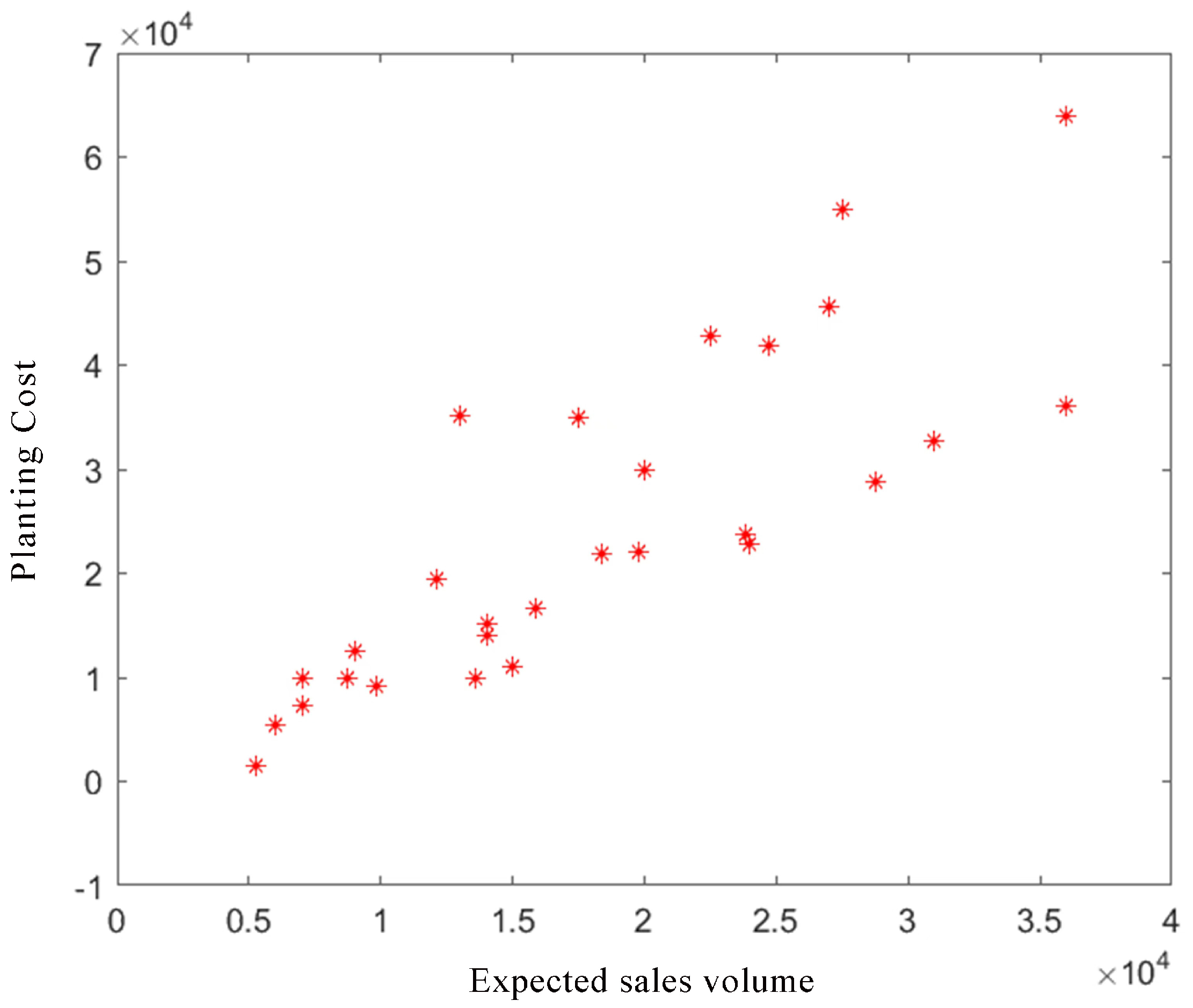
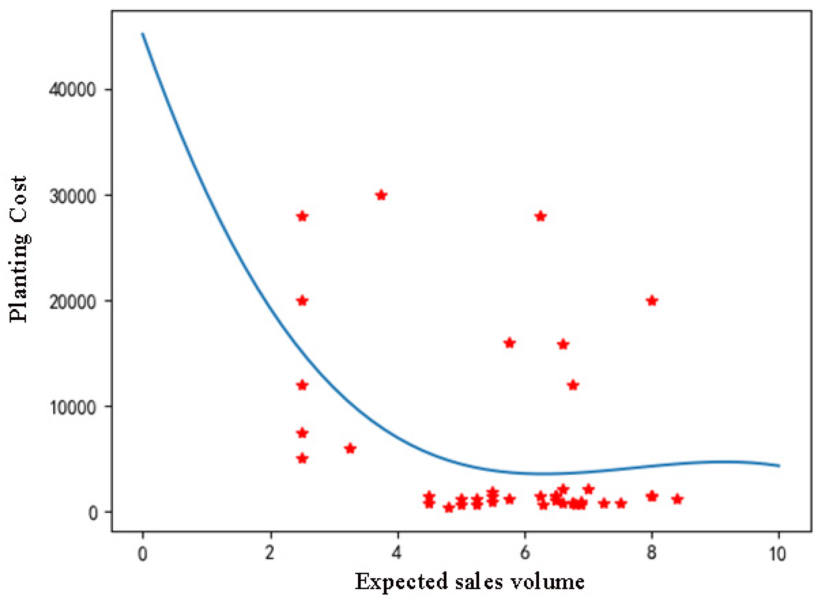
We conducted an in-depth analysis of the correlations between expected sales volume, sales price, and planting cost for grains, vegetables, and edible fungi, respectively. Our findings indicate a strong correlation between expected sales volume and planting cost for grain crops. Additionally, a robust correlation exists between expected sales volume and sales price for vegetable crops. In contrast, no significant correlation was observed between expected sales volume and either planting cost or sales price for edible fungi crops. Furthermore, grain crops serve as substitutes for vegetable and edible fungi crops while being complementary to both categories. Based on these insights, we derive specific regression equations using scatter plots that depict the relationship between expected sales volume and both sales price and planting cost. As an example, the scatter plot illustrating the relationship between expected sales volume and planting cost for grain crops is presented in Figure 12.
It is evident that the relationship between the expected sales volume of grain crops and their planting costs is not merely linear. To better fit the scatter plot, we employ a polynomial regression model for fitting. Specifically, we define the variable X t j ( j = 1, 2,…, 28) as the planting cost of the j -th type of grain crop in year t , and establish a polynomial regression model for the expected sales volume of grain crops in year Y t with X t j . The model is formulated as
X t j = X 2023 j ( 1 + 5 % ) t 2023
Y t = a 1 X t 1 + a 2 X t 2 2 + + a 28 X t 28 28
The scatter plot of the expected sales volume of vegetable crops versus their unit sales prices is demonstrated in Figure 13. It is evident that the relationship between the expected sales volume of vegetable crops and their unit sales prices is not merely linear. Therefore, we still use polynomial regression for fitting. We define the variable X t k (k = 1, 2, 3…42) as the sales price of the k -th type of vegetable crop in year t, and establish a polynomial regression model for the expected sales volume of vegetable crops in year Y t with X t k :
X t k = X 2023 k ( 1 + 5 % ) t 2023
Y t = a 1 X t 1 + a 2 X t 2 2 + + a 42 X t 42 42
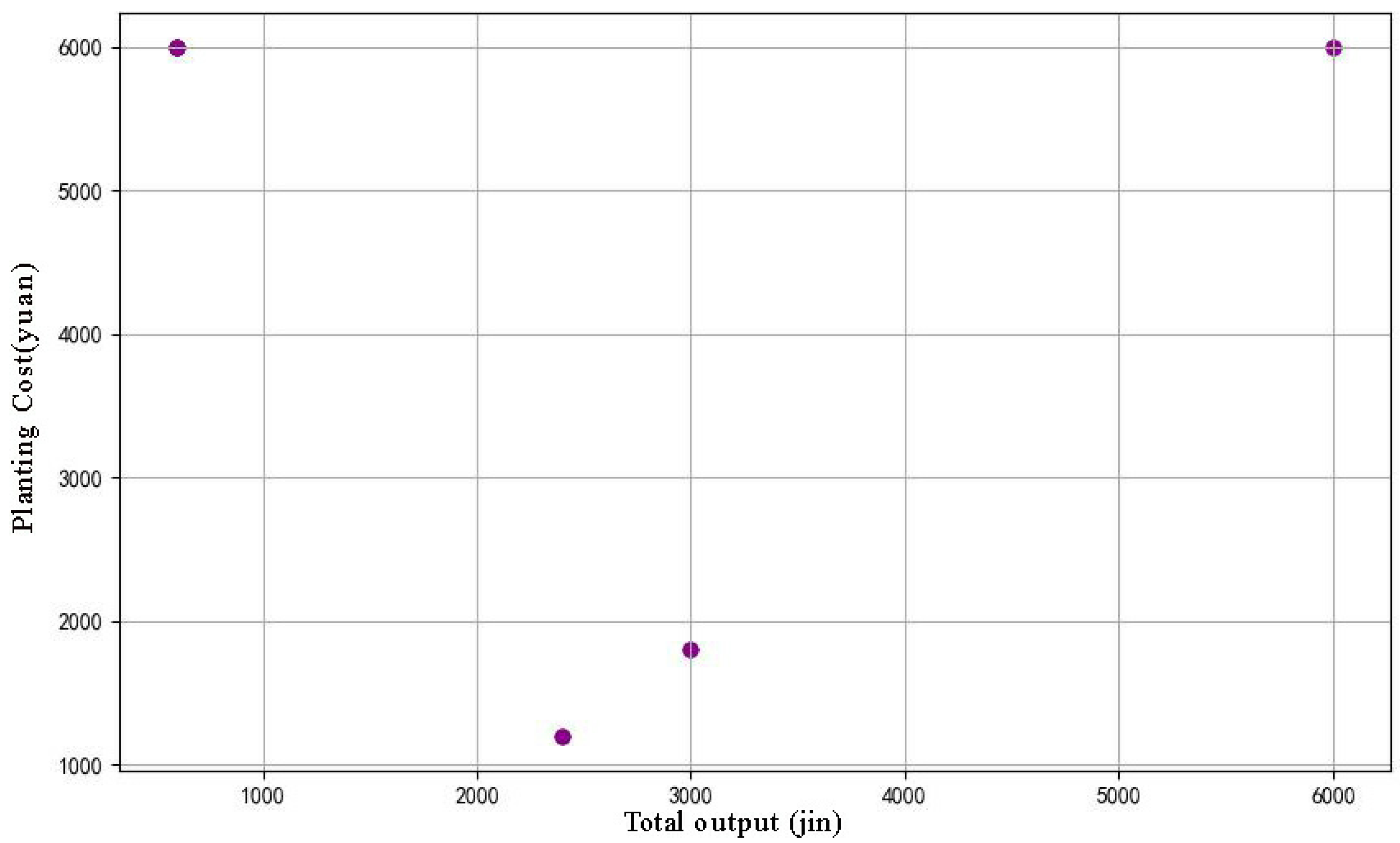
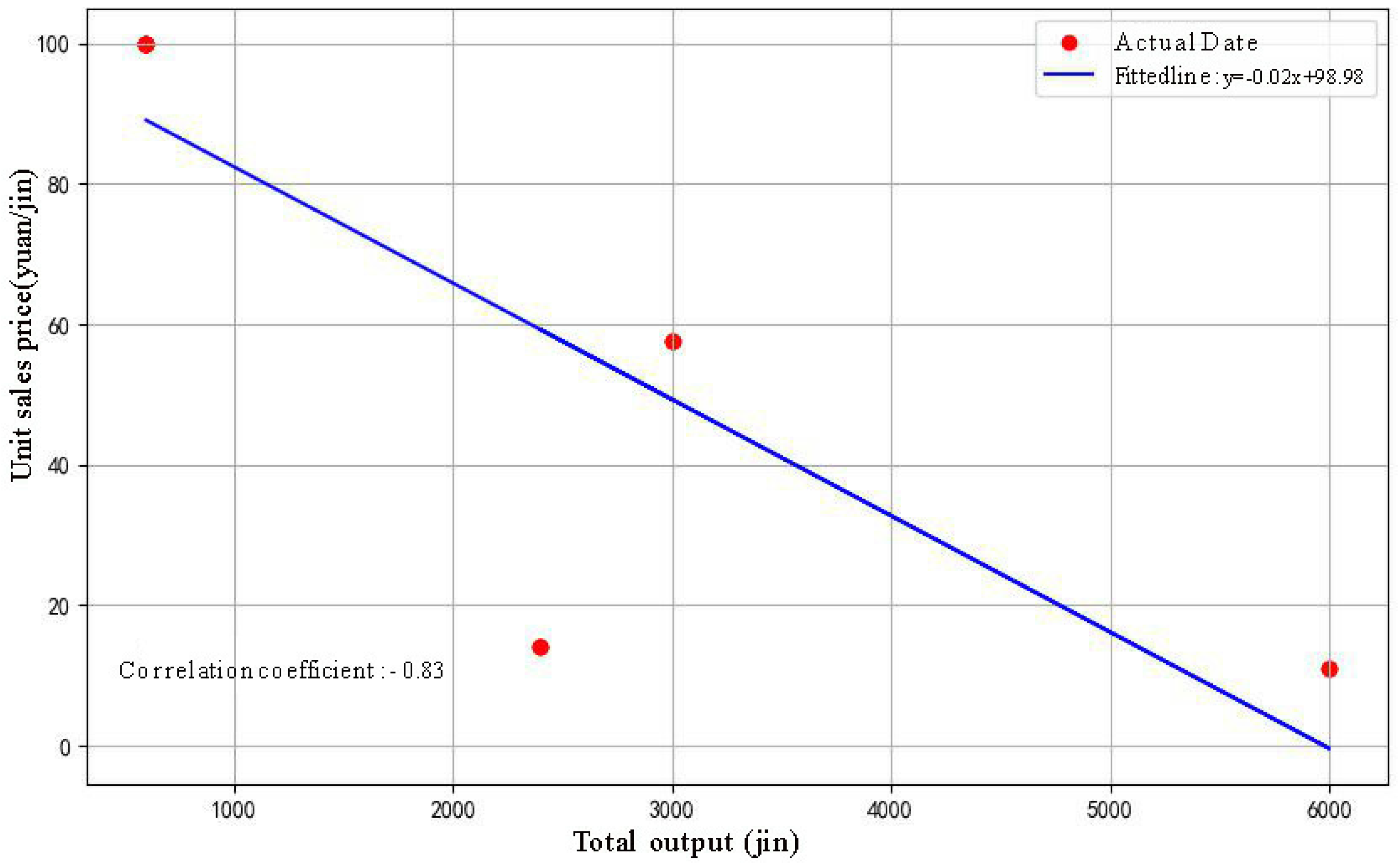
The scatter plot of the expected sales volume of edible fungi crops versus their planting costs is shown in Figure 14. We use polynomial regression for fitting. We define the variable X t k   ( k   = 1, 2, …, 42) as the sales price of the k -th type of vegetable crop in year t , and establish a polynomial regression model for the expected sales volume of vegetable crops in year Y t with X t k :
X t m = X 2023 m ( 1 + 5 % ) t 2023
Y t = a 1 X 1 + a 2 X 2 + + a 16 X 16 + b 1
The scatter plot of the expected sales volume of edible fungi crops versus their planting costs is illustrated in Figure 15.
In Figure 15, the expected sales volume of edible fungi crops has a clear linear relationship with their unit sales prices. Therefore, a linear regression is used for fitting. We define the variable X t m (m = 1, 2,…, 16) as the sales price of the m -th type of edible fungi crop in year t , and establish a linear regression equation for the expected sales volume of edible fungi crops in year Y t with X t m :
X t m = X 2023 m ( 1 + q 2 ) t 2023 + X 2023   41 ( 1 + 5 % ) t 2023
Y t = a 1 X 1 + a 2 X 2 + + a 16 X 16 + b 2
Overall, the specific objective functions for grains, vegetables, and edible fungi are as follows.
(a)
Grain crops:
X t j = X 2023 j ( 1 + 5 % ) t 2023 ,   j = 1 , 2 , 3 28 Y t = a 1 X t 1 + a 2 X t 2 2 + + a 28 X t 28 28
(b)
Vegetable crops:
X t k = X 2023 k ( 1 + 5 % ) t 2023 , k = 1 , 2 , 3 42 Y t = a 1 X t 1 + a 2 X t 2 2 + + a 42 X t 42 42
(c)
Edible fungi crops:
X t m = X 2023 m ( 1 + 5 % ) t 2023 X t m = X 2023 m ( 1 + q 2 ) t 2023 + X 2023   41 ( 1 + 5 % ) t 2023 , m = 1 , 2 , 3 , , 16 Y t = a 1 X 1 + a 2 X 2 + + a 16 X 16 + b 1 Y t = a 1 X 1 + a 2 X 2 + + a 16 X 16 + b 2
We then solve the above problems by using MATLAB (v.2021b) and present the solutions. The polynomial regression equation between the projected sales volume and cultivation cost for grain crops is formulated as
Y t = 5.0822 x 3 + 1.7936 x 2 6.3007 × 10 6 x 5.8158 × 10 11
The polynomial regression equation between the projected sales volume and unit selling price for vegetable crops is formulated as
Y t = 840.25698939 x 3 + 16329.6199537 x 2 103621.29435454 x + 221200.6225033
The polynomial regression equation between the projected sales volume and unit selling price for edible mushroom crops is formulated as
y = 12.41 x 2 + 505.4 x + 12920
To summarize, we present detailed methodologies and corresponding results for achieving the three objectives proposed in Section 1.
For the first objective, a series of constraints reflecting real-world cultivation conditions—such as land resource limitations and crop rotation requirements—are incorporated into the model. Additionally, a stochastic programming model is innovatively integrated with a robust optimization algorithm (SPM with ROA) to evaluate the total profit from crop production over a seven-year horizon. The model explicitly establishes the mathematical relationship between total profit and key decision variables (e.g., the cultivated area for each crop type), as well as stochastic variables (e.g., market price fluctuations and climate-induced yield variations). The results indicate that the optimal, normal, and the worst total profits over the seven-year period are 53.491 million yuan, 45.746 million yuan, and 38.154 million yuan, respectively.
For the second objective, an integer programming model (IPM) is synergistically integrated with a genetic algorithm (GA) to derive the optimal planting strategy. The results demonstrate that the total profit over the seven-year period is 42.6873 million yuan in Scenario A and 46.586 million yuan in Scenario B.
Regarding the third objective, heatmaps are generated to illustrate the correlations among anticipated sales volume, cultivation cost, and selling price for three major crop types. A detailed analysis of these heatmaps visually and quantitatively reveals the correlations between crop types and key driving factors like cost and price. This analysis offers critical data support for the formulation of crop planting strategies. The optimized model, informed by this analysis, yields a total profit of 55.786 million yuan.

5.3. Related Works

The interrelationship of our work with other studies in the field is discussed. For instance, Zehao Yan et al. employed a stochastic programming model (SPM) [40], which assumes that the probability distribution of uncertainties is known—for example, the paper assumes that irrigation water follows a normal distribution. However, in real-world scenarios, precise probability distributions are often difficult to obtain, and such a model may not perform well under extreme conditions. Therefore, integrating a robust optimization algorithm (ROA) can, to some extent, compensate for these limitations. Furthermore, Ratanakuakangnan et al. adopted a sequential hybrid optimization strategy by first applying stochastic programming and subsequently employing robust optimization [41]. In contrast, our method enables a synchronous coupling of the SPM and ROA, thereby reducing computational complexity. Moreover, by conducting correlation analysis using heatmaps, we provide a data-driven foundation for determining the robustness level parameter. Consequently, our methodology complements theirs and contributes a valuable addition to the existing methodological framework.

5.4. Extension of the Proposed Methods

The proposed model is configurable to accommodate the specific conditions of diverse geographical regions. This configurability is operationalized across three core layers. Firstly, the data layer involves the substitution of region-specific datasets, including soil properties (e.g., arable land, yield), climatic patterns, and market dynamics (e.g., commodity prices, sales figures). Secondly, the parameter layer necessitates the recalibration of stochastic variables, particularly the parameters defining their underlying probability distributions. Thirdly, the constraint layer requires the reconstruction of constraints, as these are often contingent on local geographical and infrastructural conditions.
Particular attention must be paid to key parameters that cannot be simply transposed in the parameter layer. For example, the stochastic climate model for the Yunnan-Guizhou Plateau must be re-specified to use an extreme value distribution to capture the occurrence of abrupt frost events, rather than relying on the normal distribution assumption valid for North China. Similarly, in the constraint layer, the functional form of the water resource constraint must be redesigned to reflect the specifics of a drip irrigation system, as is prevalent in Xinjiang. Moreover, sensitivity analysis utilizing heatmaps offers significant utility for cross-regional model adaptation. This analytical technique enables the rapid identification of critical sensitivity factors within a new context. For instance, if an analysis indicates that typhoon risk outweighs price volatility in a coastal region, the weighting factors within the objective function must be adjusted accordingly to reflect this prioritization.
When scaling the analysis to the district or municipal level, official historical data can be employed to rank the relative importance of crops and thereby identify key agricultural products for the region. For example, two specific screening methods are applicable: (a) selecting the top ten crops based on their share of local planting area, and (b) selecting the top ten crops according to their share of total profit. These methods can reduce computational demands and inherently account for climatic factors. For the latter, the reason is that crops selected are commonly well-suited to the local climatic conditions.
Furthermore, when extending the analysis to the provincial level, the province can be divided into smaller districts or municipalities as sub-regions. Calculations for each sub-region can then be conducted independently and later aggregated. The methodology applied to each sub-region remains consistent with the above two methods. To improve computational efficiency further, the number of key crops identified can be reduced, for example, from top ten to top five. Therefore, as the geographical regions increase, the number of selected crops can be decreased for computation efficiency. Through these procedures, it is feasible to derive an approximate planting strategy for major crops within larger regions.

5.5. Agricultural Resilience Analysis

Our framework incorporates a robust optimization algorithm (ROA) to enhance agricultural resilience in the face of climatic and market uncertainties. It first establishes absorptive resilience [42,43] by ensuring that profits remain above a predefined baseline, even in adverse conditions. This is achieved through the fundamental capability of the ROA to identify robust solutions in uncertain environments. Furthermore, the framework demonstrates adaptive resilience [44,45] by employing dynamic decision variables and constraints, such as crop rotation requirements, to adjust planting strategies in real time. For instance, the model can optimize the vegetable-to-mushroom ratio based on price forecasts or enforce crop rotations to mitigate the risks of continuous cropping. Finally, by analyzing crop substitution and complementarity effects, along with correlation–regression modeling, the framework supports transformative resilience [46]. This enables the system to anticipate and adapt to long-term shifts in market dynamics and environmental conditions, thereby evolving its cropping structure to sustain profitability over time.

5.6. Trade-Offs Between Profit, Soil Health, Biodiversity, and Climate

The pursuit of short-term, high economic returns often leads to unsustainable practices such as continuous monocropping of high-profit crops. However, such practices can result in soil nutrient depletion, a decline in biodiversity, and a reduction in the resilience of agricultural systems. In contrast, prioritizing ecological methods, such as implementing crop rotation or incorporating fallow periods, may temporarily reduce revenue per unit area. Nevertheless, these strategies significantly enhance the long-term sustainability of agricultural systems. Over a decade-long timeframe, ecologically sound models outperform conventional systems in cumulative benefits and show greater resilience during extreme climate events. This dynamic balance suggests that the optimal decision is not merely a single-objective maximum, but rather an ongoing trade-off between economic returns and ecological health, contingent upon specific climatic and market conditions.

6. Conclusions and Future Work

This study systematically explores the optimization of crop planting strategies with the aim of enhancing agricultural planting efficiency and economic benefits. The core innovation lies in proposing an integrated decision-making approach combining stochastic programming, robust optimization, and data-driven modeling. First, we formulated a SPM with ROA, aimed at maximizing the expected total profits from crop production over a seven-year period. This model explicitly characterizes the mathematical relationships between total profits and key decision variables (such as planting areas for various crops) as well as stochastic variables (including market price fluctuations and yield variations under climatic influences). Secondly, we incorporated a series of constraints reflecting actual planting conditions (such as land resource limitations and crop rotation requirements) into the model. To solve this complex model containing uncertainties, we innovatively integrated IPM with GA to collaboratively derive optimal planting strategies. Finally, to gain deeper insights into the key factors influencing planting decisions, we generated correlation heatmaps illustrating the relationships between expected sales volumes and both planting costs and selling prices for three major crop categories. Through detailed analysis of these heatmaps, we visually revealed and quantified the strength and patterns of correlations between different crop types and core driving factors like costs and prices, providing crucial data support for planting strategy formulation. The optimized strategy demonstrates a 16.93% increase in projected total revenue, confirming its substantial practical value.
In future work, we will elaborate on field tests and how to adapt the intelligent optimization methods to other geographical regions. Although we establish a solid theoretical foundation through mathematical modeling and computational validation, the field verification of the proposed optimization strategies in the real world remains an unsolved issue. Such field validation depends on data being collected in subsequent growing seasons, largely due to the complexities associated with crop growth cycles and long-term rotational effects. To address this gap, we have initiated a structured field experiment aimed at prioritizing the statistical evaluation of crop yields under abiotic stress conditions, such as drought or low temperatures. A definitive assessment is anticipated upon completion of two full growing cycles, which we believe will offer a meaningful basis for subsequent investigations.

Author Contributions

C.W., J.Z., T.W., and B.Z. conceived the idea; C.W., B.Z., and B.W. designed the algorithms; C.W., T.W., and Y.C. (Yishan Chen) analyzed the data; C.W., J.Z., T.W., B.Z., B.W., Y.C. (Yishan Chen), and Y.C. (Yang Chen) wrote and revised the paper. All authors have read and agreed to the published version of the manuscript.

Funding

This research was funded by the National Natural Science Foundation of China (No. 62302200), the Jiangxi Provincial Key Laboratory of Multidimensional Intelligent Perception and Control of China (No. 2024SSY03161), the Jiangxi Provincial Natural Science Foundation (No. 20232BAB212022), the Doctoral Scientific Research Foundation of Jiangxi University of Science and Technology (No. 205200100634), Open Fund for Scientific Research Platform of Jiangxi University of Science and Technology (No. 2024DWZNSZ01), and the Natural Science Basic Research Program of Shaanxi (No. 2025JC-YBQN-929).

Data Availability Statement

The data presented in this study are available on reasonable request from the corresponding author.

Conflicts of Interest

The authors declare no conflicts of interest.

Abbreviations

The following abbreviations are used in this manuscript:
SPMStochastic programming model
IPMInteger programming model
ROARobust optimization algorithm
GAGenetic algorithm

References

  1. Chen, J. Research on the Protection of Agricultural Ecological Environment and Sustainable Development Path. World Trop. Agric. Inf. 2025, 5, 72–74. [Google Scholar]
  2. Wang, C.; Dong, W.; Wang, X. Research on the Coupling and Adaptation of Agricultural Sustainable Development Strategy and Rural Revitalization Strategy. J. Anyang Norm. Univ. 2019, 4, 31–35. [Google Scholar] [CrossRef]
  3. Deng, R.; Guo, W.; Chen, W.; Zhao, C. Multi-Agricultural Machinery Collaborative Task Planning Based on Non-dominated Sorting Genetic Algorithm. J. Chin. Agric. Mech. 2025, 46, 113-119+149. [Google Scholar] [CrossRef]
  4. Tian, M.; Ni, W.; Hu, W.; Ru, H.; Zhao, W. Optimization of Crop Planting Strategies in North China Mountainous Areas Based on Linear Programming. South. Agric. 2025, 19, 73–81. [Google Scholar] [CrossRef]
  5. Tang, S.; Wang, W.; Zhang, H.; Jiang, G. Analysis of Crop Planting Strategies Based on Two-Stage Optimization. J. Smart Agric. 2025, 5, 68-74+79. [Google Scholar] [CrossRef]
  6. Meng, Z.; Wang, J. Innovation in the Path of Agricultural Sustainable Development Under the Implementation of the Rural Revitalization Strategy. Agric. Econ. 2024, 10, 15–17. [Google Scholar]
  7. Li, B. Exploration and Practice of Agricultural Sustainable Development Models under the Rural Revitalization Strategy. Hebei Agric. Mach. 2025, 4, 162–164. [Google Scholar] [CrossRef]
  8. Wang, X. Analysis of the Advantages of Intercropping and Relay Cropping in Crop Planting. Seed Technol. 2025, 43, 194–196. [Google Scholar] [CrossRef]
  9. Sacks, W.J.; Deryng, D.; Foley, J.A.; Ramankutty, N. Crop planting dates: An analysis of global patterns. Glob. Ecol. Biogeogr. 2010, 19, 607–620. [Google Scholar] [CrossRef]
  10. Zhao, Y. Analysis of Greenhouse Vegetable Planting Techniques and Pest and Disease Control Strategies. Agric. Mach. Mark. 2025, 5, 65–67. [Google Scholar]
  11. Han, E. Exploration of Crop Planting Structure Optimization. Heilongjiang Grain 2024, 12, 23–25. [Google Scholar]
  12. Kambli, A.; McGarvey, R.G. Network design for local agriculture using robust optimization. Inf. Process. Agric. 2021, 8, 469–483. [Google Scholar] [CrossRef]
  13. Xia, J.Y.; Li, S.; Huang, J.J.; Yang, Z.; Jaimoukha, I.M.; Gündüz, D. Metalearning-based alternating minimization algorithm for nonconvex optimization. IEEE Trans. Neural Netw. Learn. Syst. 2022, 34, 5366–5380. [Google Scholar] [CrossRef]
  14. Yin, Y.; Gong, H.; Chen, Z.; Tian, X.; Wang, Y.; Wang, Z.; He, K.; Miao, Q.; Chu, Y.; Xue, Y.; et al. Underestimated sequestration of soil organic carbon in China. Environ. Chem. Lett. 2025, 23, 373–379. [Google Scholar] [CrossRef]
  15. Xu, M.; Meng, X.; Liu, H. The Impact of Urbanization on Crop Planting Structure in China. Lanzhou Acad. J. 2013, 2, 141–146. [Google Scholar]
  16. Liu, F. Some Suggestions on Adjusting Crop Planting Structure. Agric. Econ. 2001, 5, 44. [Google Scholar]
  17. Zhang, Y. The Evolution of Crop Planting Structure and Rural Social Change: A Case Study of Central Hubei Rural Areas. Agric. Past Present 2005, 1, 9–14. [Google Scholar]
  18. Wang, W.H.; Zheng, J.H.; Liu, Z.; Fang, J.; Li, Z.; Wu, Q.H. Hierarchical demand response considering dynamic competing interaction based on multi-agent deep deterministic policy gradient. CSEE J. Power Energy Syst. 2025. [CrossRef]
  19. Li, J.; Zu, L.Y.; Zhong, X.L. Comparative Advantage Analysis of Crop Planting: A Case Study of Sichuan Province. Rural. Econ. 2005, 9, 47–49. [Google Scholar]
  20. Wieme, R.A.; Carpenter-Boggs, L.A.; Crowder, D.W.; Murphy, K.M.; Reganold, J.P. Agronomic and economic performance of organic forage, quinoa, and grain crop rotations in the Palouse region of the Pacific Northwest, USA. Agric. Syst. 2020, 177, 102709. [Google Scholar] [CrossRef]
  21. Wang, X.; Wang, W. Comparative Advantage Analysis of Major Agricultural Products in Yunnan’s Organic Agriculture. Contemp. Econ. 2014, 18, 72–73. [Google Scholar]
  22. Du, H.; Zhao, Y. A Review of Intelligent Algorithms for Solving Integer Programming Problems. J. Comput. Appl. Res. 2010, 27, 408–412. [Google Scholar]
  23. Zhu, H.; Liu, J.; Liu, F.; Li, T.; Wang, H. Adaptive Genetic Algorithm for Optimizing Crop Planting Structure and Resource Allocation. J. Liaoning Univ. Technol. 2019, 39, 393–396. [Google Scholar] [CrossRef]
  24. Zhang, D. Application of Genetic Algorithms in Multi-Constraint Combinatorial Optimization. J. Equip. Command. Technol. Coll. 2005, 3, 112–113. [Google Scholar]
  25. Zhang, A.; He, J. The Impact of Climate Change on Crop Growth and Coping Strategies. Rural. Sci. Exp. 2025, 5, 193–195. [Google Scholar] [CrossRef]
  26. Zhao, C.; Zhang, S. Exploring the Impact of Climate Change on Crop Breeding Strategies. Hebei Agric. Mach. 2024, 9, 94–96. [Google Scholar] [CrossRef]
  27. Zhang, H. Research on the Impact of Climate Change on Ecosystems and Agricultural Production. Agric. Disaster Res. 2023, 13, 201–203. [Google Scholar]
  28. Wang, Y. The Impact of Climate Change on Agricultural Meteorological Disasters and Pests and Coping Measures. Agric. Eng. Technol. 2021, 41, 92–93. [Google Scholar] [CrossRef]
  29. Feng, X.; Liu, D.; Zhao, J.; Si, W.; Fan, S. Impact of climate change on farmers’ crop production in China: A panel Ricardian analysis. Humanit. Soc. Sci. Commun. 2025, 12, 250. [Google Scholar] [CrossRef]
  30. Orke, A.Y.; Shanka, S.A. Analyzing the Impact of Climate Change on Crop Water Demand in the Semi-Arid Bilate Watershed, Ethiopia. Adv. Meteorol. 2025, 2025, 9466355. [Google Scholar] [CrossRef]
  31. Fan, M. The Impact of Climate Change on Crop Planting Patterns and Adaptive Strategies. Agric. Dev. Equip. 2025, 2, 160–162. [Google Scholar]
  32. Liu, J. The Impact of Climate Factors on Crop Growth and Solutions. Agric. Technol. Serv. 2017, 34, 141. [Google Scholar]
  33. Qi, L.; Zhang, M. The Impact of Agricultural Meteorological Changes on the Growth and Development of Crops in Jilin Province and Coping Measures. South. Agric. 2023, 17, 218-220+230. [Google Scholar] [CrossRef]
  34. Yu, P. Correctly Evaluating the Impact of Climate Change on Agriculture to Provide a Basis for Healthy and Stable Agricultural Development. Jilin Agric. 2016, 16, 113. [Google Scholar] [CrossRef]
  35. Li, C.; Dong, X.; Zong, Y. Analysis of Vegetable Price Trends in Hebei Province and Market Forecast for 2024. Vegetables 2024, 6, 21–27. [Google Scholar]
  36. Sabouni, M.S.; Mardani, M. Application of robust optimization approach for agricultural water resource management under uncertainty. J. Irrig. Drain. Eng. 2013, 139, 571–581. [Google Scholar] [CrossRef]
  37. Yuan, M.; Zheng, N.; Yang, Y.; Liu, C. Robust optimization for sustainable agricultural management of the water-land-food nexus under uncertainty. J. Clean. Prod. 2023, 403, 136846. [Google Scholar] [CrossRef]
  38. Mardani Najafabadi, M.; Taki, M. Robust data envelopment analysis with Monte Carlo simulation model for optimization the energy consumption in agriculture. Energy Sources Part A Recovery Util. Environ. Eff. 2024, 46, 9436–9450. [Google Scholar] [CrossRef]
  39. Ge, J.; Qiu, Y.; Wu, C.; Pu, G. A Review of Genetic Algorithms. J. Comput. Appl. Res. 2008, 25, 2911–2916. [Google Scholar]
  40. Yan, Z.; Li, M. A stochastic optimization model for agricultural irrigation water allocation based on the field water cycle. Water 2018, 10, 1031. [Google Scholar] [CrossRef]
  41. Ratanakuakangwan, S.; Morita, H. Hybrid stochastic robust optimization and robust optimization for energy planning–A social impact-constrained case study. Appl. Energy 2021, 298, 117258. [Google Scholar] [CrossRef]
  42. Usman, M.; Hameed, G.; Saboor, A.; Almas, L.K.; Hanif, M. R&d innovation adoption, climatic sensitivity, and absorptive ability contribution for agriculture TFP growth in Pakistan. Agriculture 2021, 11, 1206. [Google Scholar] [CrossRef]
  43. El Chami, D.; Daccache, A.; El Moujabber, M. How can sustainable agriculture increase climate resilience? A systematic review. Sustainability 2020, 12, 3119. [Google Scholar] [CrossRef]
  44. Cámara, J.; de Lemos, R.; Vieira, M.; Almeida, R.; Ventura, R. Architecture-based resilience evaluation for self-adaptive systems. Computing 2013, 95, 689–722. [Google Scholar] [CrossRef]
  45. Hellin, J.; Fisher, E.; Taylor, M.; Bhasme, S.; Loboguerrero, A.M. Transformative adaptation: From climate-smart to climate-resilient agriculture. CABI Agric. Biosci. 2023, 4, 30. [Google Scholar] [CrossRef]
  46. Asadzadeh, A.; Khavarian-Garmsir, A.R.; Sharifi, A.; Salehi, P.; Kötter, T. Transformative resilience: An overview of its structure, evolution, and trends. Sustainability 2022, 14, 15267. [Google Scholar] [CrossRef]
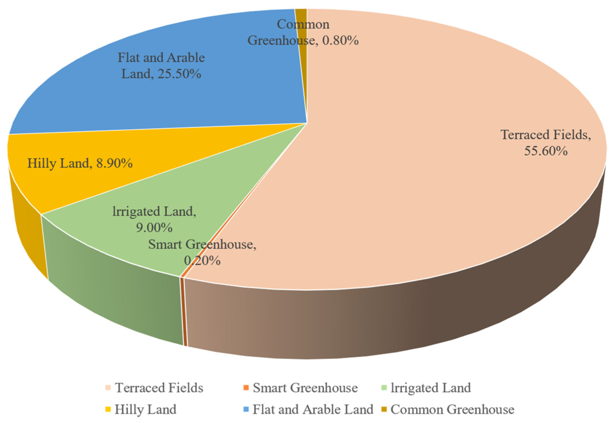
Figure 1. The proportion occupied by different types of cultivated land area.
Agriculture 15 01736 g001
Figure 2. The cultivated area of each crop.
Agriculture 15 01736 g002
Figure 4. Normal distribution of the annual change rate in expected sales volume of wheat and corn.
Agriculture 15 01736 g004
Figure 5. Partial results of the planting plan for 2024–2030.
Agriculture 15 01736 g005aAgriculture 15 01736 g005b
Figure 6. Total profits of optimization methods with different fluctuation variations.
Agriculture 15 01736 g006
Figure 7. Partial results of the optimal cultivation strategy in Scenario A.
Agriculture 15 01736 g007
Figure 8. Partial results of the optimal planting strategy Scenario B.
Agriculture 15 01736 g008
Figure 9. Heatmap of expected sales volume of grain crops versus planting cost and unit sales price.
Agriculture 15 01736 g009
Figure 10. Heatmap of expected sales volume of vegetable crops versus planting cost and unit sales price.
Agriculture 15 01736 g010
Figure 11. Heatmap of expected sales volume of edible fungi crops versus planting cost and unit sales price.
Agriculture 15 01736 g011
Figure 12. Scatter plot of expected sales volume of grain crops versus planting cost.
Agriculture 15 01736 g012
Figure 13. Relationship diagram between expected sales volume and unit price of vegetable crops.
Agriculture 15 01736 g013
Figure 14. Scatter plot of expected sales volume of edible fungi crops versus planting cost.
Agriculture 15 01736 g014
Figure 15. Scatter plot of expected sales volume of edible fungi crops versus unit sales price.
Agriculture 15 01736 g015
Table 1. Expected sales volume of each crop in 2023.
Plot IDCrop CodeCrop NameTotal Yield
A41Soybean28,800
B111Soybean22,800
C31Soybean5400
B22Black soybean21,850
B33Red bean15,200
C63Red bean7200
A54Mung bean23,800
B44Mung bean9240
B55Cowpea9875
A16Wheat64,000
Table 2. Nomenclature.
SymbolDescription
X i j The area planted with the j -th crop in the i -th plot
S i The area of the i -th plot
Q j The unit selling price of the j -th crop
r i j A binary variable indicating whether the j -th crop can be planted in the i -th plot (0 = no, 1 = yes)
C j The planting cost per unit area for the j -th crop
L j The yield per unit area of the j -th crop
X t i j The area planted with the j -th crop in the i -th plot during year t
W j The expected sales volume of the j -th crop
P i j The yield of the j -th crop in the i -th plot
P t i j The yield of the j -th crop in the i -th plot during year t
Z Total revenue over the seven-year period 2024–2030
Table 3. Changes in parameters in three fluctuation scenarios.
Fluctuation Scenarios
Robust Fluctuation VariationNormal Fluctuation VariationWorst-Case Fluctuation Variation
Parameters
The annual change rate of the expected sales volume for wheat and corn10%7.5%5%
The annual change rate of the expected sales volume for other crops5%0−5%
The annual change rate of crop yield per acre10%0−10%
The annual change rate of planting costs3%5%7%
The annual change rate of grain crop sales prices2%0−2%
The annual change rate of vegetable crop sales prices7%5%3%
The annual change rate of edible fungus prices−1%−3%−5%
Table 4. Partial results of the optimized planting strategy for the first season.
The First Season
Field NameCrop TypePlanting Area
A1Wheat80
A2Red beans55
A3Wheat35
A4Wheat72
A5Corn68
A6Corn55
B1Black beans53.8
B2Sorghum46
B3Millet40
B4Mung beans28
B5Sorghum25
Table 5. Partial results of the optimized planting strategies for the second season.
The Second Season
Field NameCrop TypePlanting Area
D1Chinese cabbage15
D2Chinese cabbage10
D3White radish14
D4Chinese cabbage5
D5
D6Carrot12
D7
D8White radish11
E1
E2
E3
Table 6. Partial results of the planting strategy in Scenario A for the first season.
The First Season
Field NameCrop TypePlanting Area
A1Wheat80
A2Millet55
A3Millet35
A4Wheat72
A5Corn68
A6Mung beans55
B1Wheat60
B2Millet46
B3Buckwheat35
B4Red beans28
B5Sorghum25
Table 7. Partial results of the planting strategy in Scenario A for the second season.
The Second Season
Field NameCrop TypePlanting Area
D1White radish15
D2Chinese cabbage10
D3Chinese cabbage14
D4Chinese cabbage6
D5White radish10
D6Carrot12
D7
D8
E1
E2
E3
Table 8. Partial results of the planting strategy in Scenario B for the first season.
The First Season
Field NameCrop TypePlanting Area
A1Mung beans80
A2Corn55
A3Climbing beans35
A4Wheat72
A5Corn68
A6Wheat55
B1Millet60
B2Sorghum46
B3Wheat40
B4Sorghum28
B5Corn25
Table 9. Partial results of the planting strategy in Scenario B for the second season.
The Second Season
Field NameCrop TypePlanting Area
D1White radish15
D2Carrot4
D3Carrot14
D4Chinese cabbage6
D5Chinese cabbage8
D6Chinese cabbage11
D7White radish22
D8Chinese cabbage20
E1
E2
E3
Table 10. Key performance metrics under all scenarios.
ScenariosSPM with ROA MethodsIPM with GA Methods
Key
Metrics
OptimalNormalWorstAB
Profit increase42.5%21.8%2.6%13.7%24.1%
Land utilization100%80.7%60.2%77.4%82.3%
Risk mitigation40.2%20%——11.9%22.1%
Table 11. Key parameters and fluctuation ranges.
Key ParametersFluctuation Ranges
Expected sales volumeWheat and corn annual growth rates5~10%
Other crops annual change rate−5~5%
Yield per acreAll crops annual change rate−10~10%
Planting costAll crops annual growth rate5%
Selling priceAnnual growth rate of vegetable crops5%
Annual decline rate of edible mushroom crops1~5%
Annual decline rate for morel mushrooms5%
Table 12. Baseline values of key parameters and total profit.
Key ParametersBaseline Values
Expected sales volumeWheat and corn annual growth rates7.5%
Other crops annual change rate0%
Yield per acreAll crops annual change rate0%
Planting costAll crops annual growth rate5%
Selling priceAnnual growth rate of vegetable crops5%
Annual decline rate of edible mushroom crops3%
Annual decline rate for morel mushrooms5%
Baseline total profit (million yuan)45.746
Table 13. Sensitivity analysis.
Key ParametersParameter FluctuationSensitivity Analysis of Profit (Million Yuan)Sensitivity Elasticity Coefficient
Expected sales volumeWheat and corn annual growth rates5%Falls to 39.812 6.8
10%Rises to 53.491
Other crops annual change rate−5%Falls to 43.3691.04
5%Rises to 48.123
Yield per acreAll crops annual change rate−10%Falls to 40.2581.2
10%Rises to 51.234
Planting costAll crops annual growth rate−2%Falls to 43.3692.6
2%Rises to 48.123
Selling priceAnnual growth rate of vegetable crops−2%Falls to 43.3692.6
2%Rises to 48.123
Annual decline rate of edible mushroom crops−2%Rises to 48.123−2.6
2%Falls to 43.369
Table 14. Complementarity–substitution effects among common crops.
Crop CategoriesHigh Substitution Complementary CombinationSubstitution CoefficientsSubstitution and Complementary Logic
GrainsBlack beans↔Red beans ↔Climb beans0.92The yield is similar, and the nutritional function is similar
Wheat↔Barley ↔Millet0.85Dry land production capacity is similar
VegetablesSweet potato↔Potato ↔Pumpkin0.78High-yield filler crops
Spinach↔Lettuce ↔Small greens0.95The growth cycle is short, and the annual output of the greenhouse exceeds 4000 catties
fungiElm yellow mushroom ↔Lentinula edodes ↔White spirit mushroom0.65Exclusive to greenhouses, but the yield varies greatly
Disclaimer/Publisher’s Note: The statements, opinions and data contained in all publications are solely those of the individual author(s) and contributor(s) and not of MDPI and/or the editor(s). MDPI and/or the editor(s) disclaim responsibility for any injury to people or property resulting from any ideas, methods, instructions or products referred to in the content.