Can Agricultural Sustainable Development and Rural Industrialization Be Achieved Simultaneously? The Practice of Rural Industrial Integration from China

Abstract

Improving agricultural eco-efficiency (AEE) plays a critical role in fulfilling agriculture sustainable development goals (SDGs). China’s agriculture-led Rural Industrial Integration (RII) seeks to synergize rural industrialization with agricultural sustainability, yet its impact on AEE remains underexplored. Using a 2008–2022 panel of 285 prefecture-level cities in China, this study uses a series of econometric methods to empirically verify the impact of RII on AEE. The coefficient of RII under the fixed effect model is 0.366, indicating that it has a significant positive impact on AEE, which remains valid after robustness tests such as the instrumental variable method and the use of the “Rural Industrial Integration Development Demonstration County” pilot as a quasi-natural experiment. Mechanism tests show that rural labor transfer, agricultural technology innovation, and agricultural carbon emissions play an important role in mediating the impact of RII on AEE. RII has a negative spatial spillover effect on AEE, with a coefficient of −2.280. In addition, the impact of RII on AEE also varies under the heterogeneity of regions and development models. This study provides new evidence that China’s RII practices can promote sustainable agricultural development, deepens theoretical understanding of the impact of RII on AEE, and provides a reference for future policy implementation.

1. Introduction

Agriculture serves as a fundamental pillar for human existence and progress by providing food, animal feed, fuel, and a variety of raw materials. With global population growth and evolving dietary patterns, the demand for food and agricultural products is becoming increasingly urgent [1]. The UN projects that the global population will peak at 10.3 billion by the 2080s, and expanding agricultural production is key to meeting the food needs of a growing population. This can be achieved either through intensification—such as increased use of fertilizers, pesticides, water, or improved management practices—or by expanding arable land [2]. However, both approaches consume substantial resources and may lead to environmental degradation, exhibiting characteristics of regional relevance, spatial spillover, and negative externalities [3]. Given the strong interdependence between agriculture and the environment [4], under the conflict between limited resource constraints and increasing food demand, spending fewer resources and achieving cleaner outputs through improving agricultural ecological efficiency (AEE) helps achieve sustainable development goals (SDG) [5]. Sustainable agriculture requires that farmers continue producing crops and livestock without degrading environmental or resource bases, while maintaining economic viability and social stability [6]. Therefore, improving both economic and ecological efficiency in agricultural production lies at the core of sustainable agricultural development.

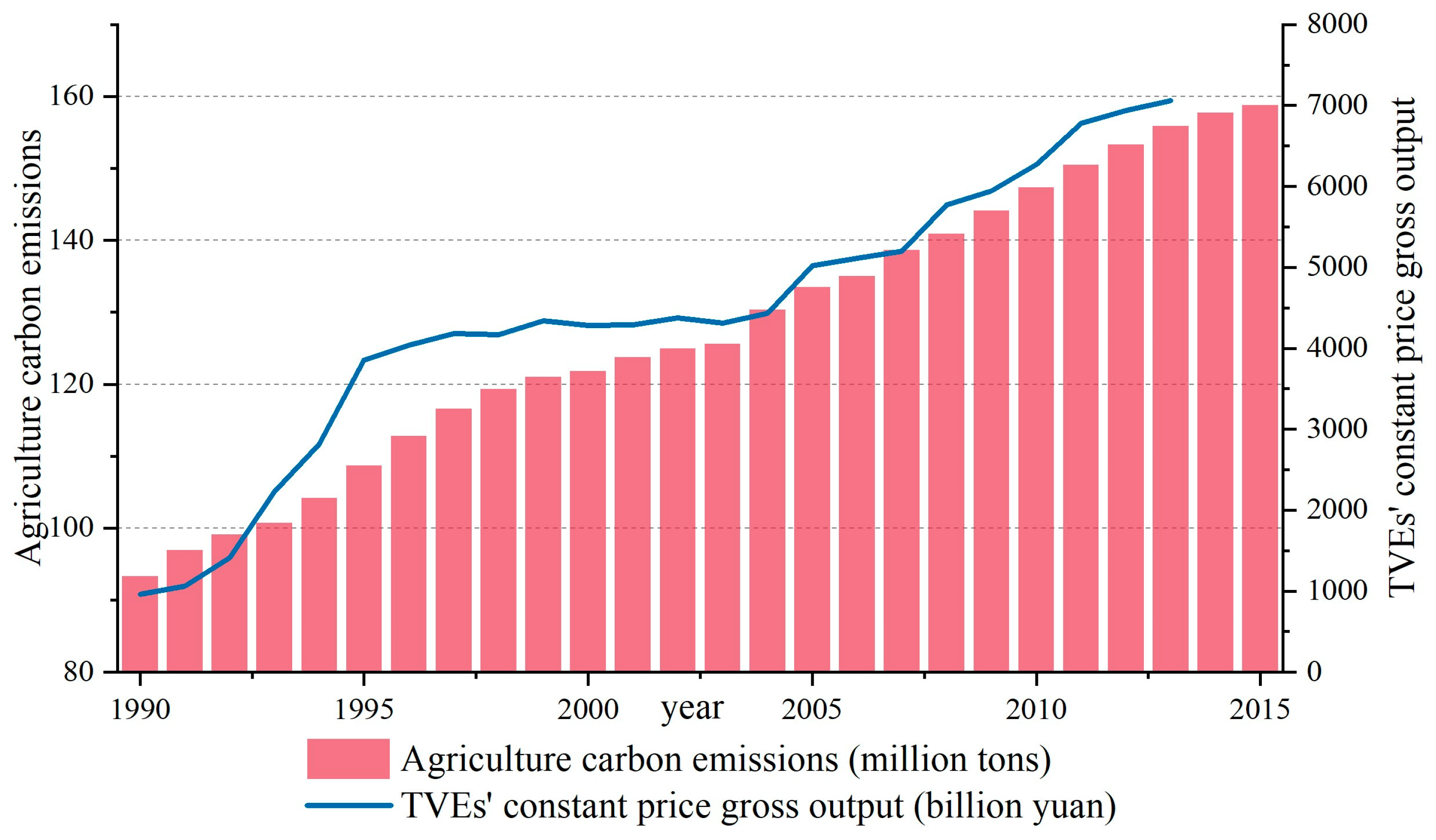
Although rural regions are essential for sustaining agricultural production, many in developing countries continue to suffer from persistent economic underdevelopment and inadequate living standards. In some cases, rural industrialization has driven rapid economic growth and increased household incomes, but the accompanying environmental consequences are mixed and often concerning [7]. Environmental issues such as carbon emissions are closely linked to rural human development [8], highlighting the inherent tension between agricultural sustainability and rural development. Since reform and the opening-up policy, township and village enterprises (TVEs) in China have undergone remarkable growth and contributed significantly to rural industrial development. However, this industrialization has not led to corresponding improvements in agricultural production conditions. Instead, agricultural expansion has been accompanied by environmental degradation, without notable gains in agricultural eco-efficiency. Figure 1 shows the changes in agricultural carbon emissions during the development process of TVEs, indicating a high correlation between the two.

As the world’s largest developing nation, China confronts challenges related to uneven development between its urban and rural regions, as well as disparities between the industrial and agricultural sectors. In response, China has implemented the Rural Revitalization Strategy, emphasizing industrial revitalization as the cornerstone and essential element for overall rural revitalization. Within this strategy, thriving rural industries are identified as the primary goal, and Rural Industrial Integration (RII) serves as a vital means to achieve rural industrial prosperity [9]. In 2015, the Chinese government first advocated for the integration of the three rural industries, with the goal of improving factor allocation between industry and agriculture and across urban and rural areas, ultimately enhancing rural incomes and addressing urban-rural development imbalances [10]. Since then, the Chinese government has frequently underscored the importance of RII in official documents, supported its development through policy incentives, and identified a number of pilot demonstration counties for rural industrial integration development in 2016. RII has promoted diverse innovative agricultural forms, including internet plus agriculture and multifunctional agricultural practices [11], helping to address challenges such as resource scarcity and technological backwardness in traditional agriculture. Unlike conventional rural industrialization, RII focuses on blending agriculture with other industries, encouraging the growth of secondary and tertiary sectors while achieving optimal allocation of resources and factors across different sectors [12]. Therefore, under the dual objectives of improving rural livelihoods and achieving agricultural sustainability, studying the rural transformation process of China and analyzing the impact of RII on AEE holds significant practical value and offers valuable insights for developing countries seeking to balance environmental protection with economic growth.

This study focuses on the following key questions: (1) Can China’s RII practices achieve coordinated development between rural industrialization and sustainable agriculture? That is, while achieving rural industrialization, can RII improve AEE and thus promote sustainable agricultural development? (2) Can the impact of RII on AEE be empirically verified? Are there spatial spillover effects associated with RII’s influence on AEE? (3) What is the specific mechanism by which RII affects AEE, and what are the underlying pathways? (4) Does the impact of RII on AEE exhibit heterogeneity? The findings of this study aim to address these questions and reveal the underlying mechanisms, thereby providing scientific evidence to inform policy decisions that support both sustainable agricultural development and rural industrial progress. The structure of the remaining part of the article is as follows: Section 2 reviews the relevant research literature; Section 3 conducts theoretical analysis and proposes hypotheses; Section 4 introduces the model methods and variable selection; Section 5 analyzes and discusses the results; and Section 6 presents conclusions and implications.

2. Literature Review

Ecological efficiency has become a valuable tool for assessing sustainability, as it directly links environmental impacts with economic performance and has been extensively utilized in agriculture [13,14]. AEE denotes the capability of agricultural production to deliver high-quality outputs and services within the limits of the agroecosystem’s carrying capacity, while minimizing resource depletion and environmental harm [15]. Improving AEE is essential for achieving the sustainable development goals (SDGs) and maintaining food security. Various methods exist to measure AEE, with stochastic frontier analysis (SFA) and data envelopment analysis (DEA) being the most commonly employed due to their ability to produce highly correlated results in most cases [16,17]. DEA, a non-parametric method, is particularly suitable for evaluating ecological efficiency because it does not require a pre-specified production function and allows for multiple inputs and outputs. For instance, Liu et al. [18] employed super SBM model to evaluate interprovincial AEE levels across Chinese provinces and examined their spatial characteristics. Yang et al. [19] argued that incorporating agricultural carbon emissions as undesirable outputs provides a more accurate representation of AEE in China. Studies on AEE have been conducted at the micro level focusing on farms [20], the regional or meso level [21], and the national or macro level [22].Given that AEE encompasses agricultural production, economic growth, and ecosystem services, many factors have been found to influence it, including urbanization [18], resource endowments [23], agri-environmental schemes [24], and so on.

Previous studies have mainly explored the factors influencing AEE from the angles of socioeconomic development and policy measures. Despite growing interest in rural development, the specific contribution of rural industrialization has received limited scholarly attention. Studies investigating the effects of macro-level industrial development on ecological efficiency have predominantly centered on industrial agglomeration [25], industrial structure and upgrading [26], and industry integration [27]. and the impact on ecological efficiency often exhibits significant spatial correlations [28,29]. Despite this, the link between rural industrial development and AEE remains underexplored, with limited empirical evidence available, and this research aims to bridge that theoretical and empirical void.

Rural industrialization is intended to stimulate economic growth and enhance farmers’ incomes. Long et al. [30] indicate that rural regions in eastern coastal China have leveraged their locational advantages to develop processing industries, trade, and tourism, thereby achieving rural industrialization and prosperity. However, such regions are often deeply integrated into the urbanization process and are more likely to benefit from development opportunities [31]. This model of rural industrial development, which is not directly connected to agriculture, is difficult to replicate in less advantaged areas. For decades, China’s urban-biased development policies have concentrated resources in urban areas, contributing to gradual decline of rural regions [32]. To reverse this trend, the Chinese government introduced the Rural Revitalization Strategy, placing strong emphasis on rural industrial development and the advancement of RII as essential means to improve farmers’ livelihoods and reduce the urban–rural divide [33]. Unlike the traditional approach of establishing urban-type industries in rural areas, RII focuses on rural contexts and is closely linked to agriculture and farmers [34]. The concept of industrial integration remains loosely defined in academic discourse. Most scholars suggest that integration blurs, narrows, or even dissolves industrial boundaries, thereby enhancing industrial performance through collaboration and innovation [35]. It also strengthens the linkages between products and services [36] and fosters the development of more advanced industrial structures [37]. RII also refers to the cross-sectoral and intensive allocation of capital, technology, and resources, facilitating the integration of agriculture, industry, and services, with the ultimate goal of extending agricultural value chains and increasing farmers’ incomes [12]. Currently, there is no standardized method for measuring RII. Existing studies employ various approaches such as Herfindahl Index [38] and composite index methods [39]. Promoting RII has accelerated the development of non-agricultural industries in rural areas; however, research on rural industrial integration and its impact on AEE remains limited. The underlying mechanisms linking rural development and agricultural sustainability have yet to be systematically explored or empirically tested. To fill existing research gaps, this study develops a theoretical model to explain the RII and AEE relationship and conducts empirical analysis to assess the alignment between rural industrialization and sustainable agriculture.

This study utilizes econometric modeling to investigate the effects of RII on AEE in China, thereby revealing the connection between rural industrialization and sustainable agriculture. Building upon the existing literature, this research makes several innovative contributions. First, it constructs a novel theoretical framework grounded in industrial structural transformation and producer behavior, interpreting the mechanisms through which RII influences AEE from the perspectives of factor mobility, technological integration, and environmental externalities. Second, to strengthen the reliability of the empirical analysis, an extensive panel dataset encompassing 285 prefecture-level Chinese cities over 15-year period is utilized in this study. Third, based on insights from previous studies, this research develops a new composite index to measure RII at the prefecture level, aiming to capture the multidimensional nature of RII more accurately. Fourth, by introducing spatial econometric model, verify spatial spillover effects of RII on AEE.

3. Theoretical Mechanisms and Hypotheses

RII is based on agriculture and intensively allocates various capitals, technologies, and resources across borders to integrate agricultural production, agro-processing and marketing, cultural tourism, and services to foster close linkages and coordinated development among rural industries in primary, secondary, and tertiary [34]. Although primary objective of RII is to promote rural economic growth, its close linkage with agriculture facilitates the flow and spread of production factors and technological knowledge between agriculture and other industries, ultimately influencing agricultural production processes. The specific mechanisms are illustrated in Figure 2. Optimization of factor allocation and reduction of negative externalities helps promote the enhancement of AEE, and this impact may also cross geographical boundaries to generate spatial spillover effects. For this reason, we propose Hypothesis 1:

Hypothesis 1.

Promoting the development of RII can enhance AEE.

First, RII will enable the flow of labor, capital (machinery, fertilizer, agriculture, etc.) and land factors between agriculture and other industries, thereby improving resource allocation efficiency. On one hand, RII promotes industrial development, which increases employment opportunities and raises farmers’ incomes [38]. This elevates labor opportunity costs for agricultural producers, resulting in a decreased agricultural labor supply. Consequently, producers are more likely to substitute labor with other inputs, demonstrating a substitution effect. For semi-operating farmers who earn non-agricultural income, enhanced capital endowment encourages additional capital investment, thus generating an income effect [40,41]. These shifts result in increasing output elasticity of capital inputs (machinery, fertilizers and pesticides), and the output elasticity of labor decreases [42]. Increased use of agricultural machinery can improve green efficiency [43], but the application of fertilizers and pesticides directly increases pollution and carbon emissions, and excessive use also reduces AEE. On the other hand, RII drives non-agricultural land use in rural areas, leading to a reduction in cultivable land and a greater dependence on substituting inputs. Nonetheless, RII-induced non-farm employment may promote farmland transfer [44], leading to land consolidation and scale-oriented agricultural operations [45], which can in turn enhance AEE. Among these factor flows, RII directly promotes labor transfer, provides non-agricultural employment opportunities in rural areas, and thus increases farmers’ incomes. Increased farmers’ incomes lead to increased inputs of mechanized fertilizers and pesticides in agricultural production, while non-agricultural employment facilitates land transfer. These lead to the flow of various factors between the agricultural and non-agricultural sectors. Therefore, we propose Hypothesis 2:

Hypothesis 2.

RII can promote rural labor transfer, thereby affecting the improvement of AEE.

Second, RII promotes technological integration among primary, secondary, and tertiary industries, allowing agricultural production to benefit from the positive externalities associated with such integration, thereby facilitating technological progress. The increased demand for transportation and logistics induced by RII stimulates the supply of public infrastructure. In regions with more advanced industrial development, local governments are more likely to enhance public service provision. Supported by favorable policies and fiscal transfers, these regions often experience improvements in transportation infrastructure [46]. Improvements in infrastructure have facilitated the flow of various factors and the spread of knowledge, effectively promoting technological advancement, thus directly enhancing AEE [19]. RII also promotes cross-industry dissemination of knowledge and technology, further fostering innovation. For example, the application of digital technologies [47] is becoming increasingly prevalent in agricultural product marketing and rural tourism promotion. Through RII, these technologies are more likely to spill over into agricultural activities, enabling the adoption of new technologies and innovations in farming practices. The technological advancement driven by knowledge diffusion enhances agricultural productivity and contributes to improvements in AEE [48]. We propose Hypothesis 3:

Hypothesis 3.

RII can improve AEE by promoting agricultural technology innovation.

Third, RII helps internalize environmental externalities and achieves the joint maximization of economic and environmental utility, thereby reducing pollution and carbon emissions. Through industrial integration, the primary, secondary, and tertiary sectors become interlinked and jointly profitable. As a result, rural regions prioritize maximizing total returns rather than maximizing profits from individual sectors. First, RII extends the agricultural value chain, expands market access, and promotes brand development, which boosts the value of agricultural outputs and contributes to sales stability, and this process can benefit agriculture by reducing transaction costs [34]. These changes raise quality standards for agricultural raw materials. High-value green and organic agricultural products often require strict control of pollution and fertilizer use during production. Such organic farming practices can reduce agricultural carbon emissions and enhance AEE [49]. Moreover, RII diversifies agricultural functions by fostering agriculture-based rural tourism. The development of tourism creates demand for high environmental quality, which in turn imposes constraints on agricultural pollution and carbon emissions. This environmental constraint positively contributes to improvements in AEE [50]. We propose Hypothesis 4:

Hypothesis 4.

RII can reduce agricultural carbon emissions, thereby improving AEE.

RII may not only directly influence local AEE but also exhibit spatial correlation, potentially generating spillover effects on AEE in neighboring regions. Industrial integration improves the efficiency of regional resource allocation and advances the comprehensive integration of organizations, markets, and technologies. Importantly, such integration is not confined to a single locality. For instance, market expansion resulting from RII can attract factor inflows from nearby areas and provide more products, thereby reducing transaction costs and generating positive externalities across regions, this constitutes the spatial spillover effect of RII [51]. However, RII can also have a negative spatial impact on the AEE of other regions, exhibiting a “siphon effect.” Regions with high AEE levels can generate greater returns, which attracts various resource factors from neighboring regions, negatively impacting the AEE of other regions [52]. These influences are all possible and they may affect the surrounding areas in different ways, so we propose Hypothesis 5:

Hypothesis 5.

RII affects AEE in neighboring regions through spatial spillover effects.

4. Materials and Methods

4.1. Model Design

4.1.1. Fixed Effects Model

We begin with a baseline regression analysis using a two-way fixed effects approach to explore the influence of RII on AEE. The model is chosen because it effectively accounts for unobserved differences among regions and temporal variations. Empirical specification is as follows:

$${\mathrm{A}\mathrm{E}\mathrm{E}}_{\mathrm{i}\mathrm{t}}={\mathsf{\alpha }}_0+{\mathsf{\alpha }}_1{\mathrm{R}\mathrm{I}\mathrm{I}}_{\mathrm{i}\mathrm{t}}+{\mathsf{\alpha }}_2{\mathrm{X}}_{\mathrm{i}\mathrm{t}}+{\mathsf{\mu }}_{\mathrm{i}}+{\mathsf{\delta }}_{\mathrm{t}}+{\mathsf{\epsilon }}_{\mathrm{i}\mathrm{t}}$$

(1)

Equation (1) where ${\mathrm{A}\mathrm{E}\mathrm{E}}_{\mathrm{i}\mathrm{t}}$ denotes agriculture eco-efficiency, ${\mathrm{R}\mathrm{I}\mathrm{I}}_{\mathrm{i}\mathrm{t}}$ indicates the degree of rural industrial integration, and ${\mathrm{X}}_{\mathrm{i}\mathrm{t}}$ includes various control variables, $\mathsf{\alpha }$ is the estimated coefficients, ${\mathsf{\mu }}_{\mathrm{i}}$ stands for individual fixed effects, ${\mathsf{\delta }}_{\mathrm{t}}$ indicates time fixed effects, and ${\mathsf{\epsilon }}_{\mathrm{i}\mathrm{t}}$ refers to the random disturbance term.

4.1.2. Mediation Effect Model

In order to examine the mechanism of RII’s effect on AEE, we used a mediation effect model for analysis. Following the approach of Jiang [53], the specific model is as follows:

$${\mathrm{M}}_{\mathrm{i}\mathrm{t}}={\mathrm{a}}_0+{\mathrm{a}}_1{\mathrm{R}\mathrm{I}\mathrm{I}}_{\mathrm{i}\mathrm{t}}+{\mathrm{a}}_2{\mathrm{X}}_{\mathrm{i}\mathrm{t}}+{\mathsf{\mu }}_{\mathrm{i}}+{\mathsf{\delta }}_{\mathrm{t}}+{\mathsf{\epsilon }}_{\mathrm{i}\mathrm{t}}$$

(2)

$${\mathrm{A}\mathrm{E}\mathrm{E}}_{\mathrm{i}\mathrm{t}}={\mathrm{b}}_0+{\mathrm{b}}_1{\mathrm{R}\mathrm{I}\mathrm{I}}_{\mathrm{i}\mathrm{t}}+{\mathrm{b}}_2{\mathrm{M}}_{\mathrm{i}\mathrm{t}}+{\mathrm{b}}_3{\mathrm{X}}_{\mathrm{i}\mathrm{t}}+{\mathsf{\mu }}_{\mathrm{i}}+{\mathsf{\delta }}_{\mathrm{t}}+{\mathsf{\epsilon }}_{\mathrm{i}\mathrm{t}}$$

(3)

M is the mediating variable (rural labor transfer, agricultural technological innovation and agricultural carbon emissions), ${\mathrm{A}\mathrm{E}\mathrm{E}}_{\mathrm{i}\mathrm{t}}$ and ${\mathrm{R}\mathrm{I}\mathrm{I}}_{\mathrm{i}\mathrm{t}}$ are the dependent and independent variables, a and b are the coefficients, ${\mathsf{\mu }}_{\mathrm{i}}{\mathsf{\delta }}_{\mathrm{t}}{\mathsf{\epsilon }}_{\mathrm{i}\mathrm{t}}$ are fixed effects and disturbance terms. Equation (2) first tests the effect of RII on M, and then uses Equation (3) to test the effect of M on AEE.

4.1.3. Spatial Measurement Model

Additionally, to explore the spatial effects of RII on AEE, a general spatial econometric model is developed for verification. The model specification is

$${AEE}_{it}=\rho W_{it}{AEE}_{it}+{\beta }_1{RII}_{it}+{\phi }_1{W}_{it}{RII}_{it}+{\beta }_2{X}_{it}+{\phi }_2{W}_{it}{X}_{it}+{\mu }_i+{\delta }_t+{ϵ}_{it}$$

(4)

$${ϵ}_{it}=\lambda W_{it}{ϵ}_t+{\mathsf{\epsilon }}_{\mathrm{i}\mathrm{t}}$$

(5)

Equations (4) and (5) are specified as follows: ${AEE}_{it}$ and ${\mathrm{R}\mathrm{I}\mathrm{I}}_{\mathrm{i}\mathrm{t}}$ are the dependent and independent variables; $W_{it}$ denotes the spatial weight matrix; $\rho$ is the spatial autoregressive coefficient; $\beta$ represents the estimated coefficients of the explanatory variables; $\phi$ indicates the coefficients for the spatial lag terms of the explanatory variables; ${\mu }_i$ and ${\delta }_t$ correspond to individual and time fixed effects; ${ϵ}_{it}$ is the spatial error term; $\lambda$ is the coefficient of the spatial errors; and ${\mathsf{\epsilon }}_{\mathrm{i}\mathrm{t}}$ represents the random error term. For the general spatial econometric model mentioned above, the model simplifies to spatial lag model (SLM), when $\phi =0$, $\lambda =0$; the model degenerates into spatial error model (SEM) when $\rho =0$, $\phi =0$; and the model becomes spatial Durbin model (SDM) when $\lambda =0$. For robustness checks, the regression incorporates geographic distance, adjacency, and economic distance matrices.

4.2. Variable Selection

4.2.1. Explained Variable

This study adopts broadly defined agriculture (agriculture, forestry, animal husbandry and fishery) as its research focus, applies the super-efficiency SBM model to measure AEE. The super-efficiency SBM model, as proposed by Tone [54], extends the standard SBM framework by allowing the ranking of efficient DMUs on the production frontier. The model is formulated as follows:

$$Min\delta ={\displaystyle \frac{1}{m}}\sum _{i=1}^m\left({\displaystyle \frac{\overline{x}}{x_{ik}}}\right)/{\displaystyle \frac{1}{r_1+r_2}}\left({\displaystyle \sum _{s=1}^{r_1}}{\displaystyle \frac{\overline{y^d}}{y_{sk}^d}}+{\displaystyle \sum _{q=1}^{r_2}}{\displaystyle \frac{\overline{y^u}}{y_{qk}^u}}\right)$$

(6)

$$s.t.\left\{\begin{array}{c}\overline{x}\ge {\displaystyle \sum _{j=1,\ne k}^n}{x}_{ij}{\lambda }_j;\overline{y^d}\le {\displaystyle \sum _{j=1,\ne k}^n}{y}_{sj}^d{\lambda }_j;\overline{y^d}\ge {\displaystyle \sum _{j=1,\ne k}^n}{y}_{qj}^d{\lambda }_j;\overline{x}\ge x_k;\overline{y^d}\le y_k^d;\overline{y^u}\ge y_k^u;\\ {\lambda }_j\ge \mathrm{0,1},2,\dots ,m;j=\mathrm{1,2},\dots ,n,j\ne 0;s=\mathrm{1,2},\dots ,r_1;q=\mathrm{1,2},\dots ,r_2;\end{array}\right.$$

(7)

Assume there are $n$ DMUs, each with $m$ inputs, $r_1$ desirable outputs, and $r_2$ undesirable outputs, $x$, $y^d$, and $y^u$ denote the corresponding input, desirable output, and undesirable output matrices, $\overline{x}$ $\overline{y^d}$ $\overline{y^u}$ are their average, variable $\delta$ represents the eco-efficiency score.

AEE is estimated using labor, capital, and land as inputs. Labor is measured by the number of primary industry employees; capital includes agricultural machinery power, fertilizer use, and effective irrigation area; land is represented by total sown area. Desirable output is represented by gross value of agriculture, forestry, animal husbandry, and fishery. Undesirable output is represented by agricultural carbon emissions. The specific indicator variables are shown in

Table 1. The measure of AEE.

Indicator Type	Variable	Specific Indicators	Units
Input	Labor	The number of primary industry employees	10,000 persons
	Machinery	Total agricultural machinery power	10,000 kW
	Fertilizer	Chemical fertilizer use	10,000 tons
	Irrigation	Effective irrigation area	1000 hectares
	Land	Total sown area	1000 hectares
Desirable output	Output value of agriculture	Gross value of agriculture, forestry, animal husbandry, and fishery	100 million yuan
Undesirable output	Agricultural carbon emissions (ACE)	Estimated ACE based on agriculture inputs	10,000 tons

.

ACE are calculated based on six emission sources, obtained by summing the products of each source and its corresponding emission coefficient as follows:

$$ACE={\sum }_{i=1}^6{C}_i={\sum }_{i-1}^6{E}_i\times {\theta }_i$$

(8)

$ACE$ denotes agricultural carbon emissions, $E_i$ denotes the sources of agricultural carbon emissions, including fertilizer use, pesticide use, agricultural film use, land tillage, irrigation power and agricultural machinery, ${\theta }_i$ is the carbon emission factor of each source, the carbon emission factors of fertilizer, pesticide, agricultural film, land tillage, irrigation power, and agricultural machinery are 0.8956 kg/kg, 4.9341 kg/kg, and 5.18 kg/kg, 312.6 kg/hm², 266.48 kg/hm² and 0.18 kg/kw, respectively [55].

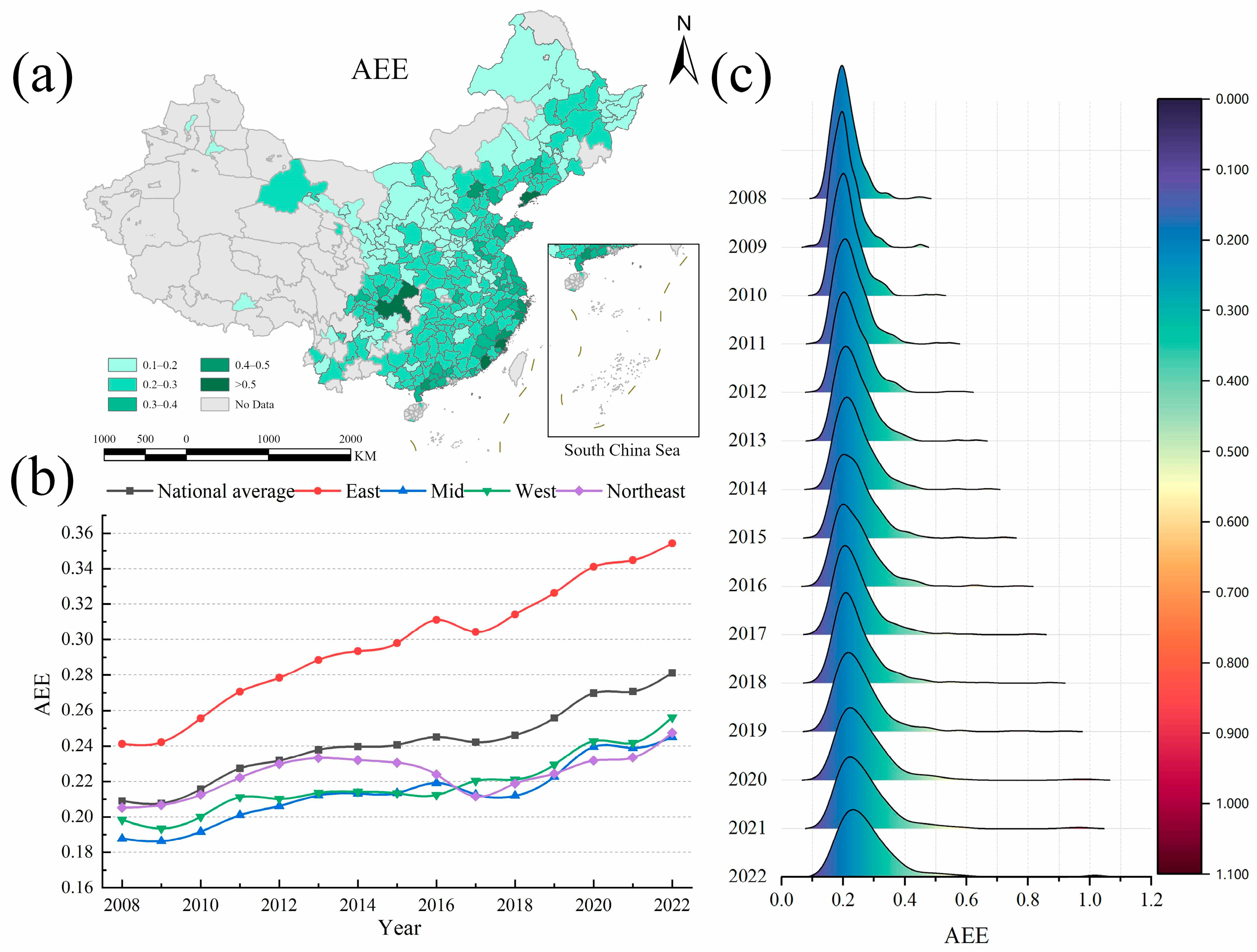
The spatial distribution and temporal evolution of AEE are shown in Figure 3. From Figure 3a, high AEE values are primarily concentrated in the eastern coastal areas, while the AEE level in the western inland areas is significantly lower. In Figure 3b, the AEE evolution trends of various regions are similar, with the AEE growth in the northeastern region showing a decline; In Figure 3c, the overall distribution of AEE shifts gradually to higher levels, but the growth is less, while the growth in high AEE regions is greater, and regional differences are gradually expanding.

4.2.2. Key Explanatory Variable

The key explanatory variable examined is RII. Although there is no standardized system to measure RII, most research develops composite indicators covering key dimensions such as industry chain extension, multifunctional expansion, service integration, and technology penetration [56]. These dimensions offer an integrated assessment of agriculture-driven RII, capturing aspects such as the vertical extension of agricultural value chains, inter-industry linkages, and technological advancement in agriculture. We measure RII based on these dimensions. Industrial chain extension reflects the development of the secondary industry in rural areas, multifunctional expansion and service integration reflect the development of the tertiary industry, and technological penetration reflects the technological level of the primary industry.

Table 2. Rural industrial integration indicator system.

First-Level Indicators	Second-Level Indicators	Tertiary Indicators	Calculation Method of Indicators	Direction
RII	Industry chain extension	Primary industry output value percentage	Primary industry output value/GDP	−
		Development of agricultural product processing industry	Number of agricultural product processing enterprises	+
		Agricultural product processing industry production level	Agricultural product processing industry output value/Primary industry output value	+
		Development of farmers’ cooperatives	Number of cooperatives	+
	Multifunctional expansion	Leisure agriculture development	Number of leisure and tourism enterprises	+
		Rural tourism development	Number of beautiful leisure villages in China	+
		Development of facility agriculture	Area of facility agriculture/Sown area of farmland	+
	Service industry integration	Agricultural supporting industry development	Number of enterprises in agricultural supporting industry	+
		Agricultural service industry output value percentage	Output value of agricultural service industry/Total output value of agriculture	+
	Technology penetration	Degree of agricultural mechanization	Total power of agricultural machinery/Sown area of farmland	+
		Irrigation level of farmland	Irrigated area/Sown area of farmland	+
		Fertilizer application intensity	Fertilizer application amount/Sown area of farmland	−
		Rural electricity consumption	Electricity usage in rural areas	+
		Village roads	Country road mileage	+

presents the specific indicators. Due to data availability, variables such as agricultural product processing output value, facility agriculture area, rural electricity consumption, and country road length are only obtained at the provincial level. This study selects 14 specific indicators across the four dimensions and uses the entropy-weighted TOPSIS method to construct the RII index system.

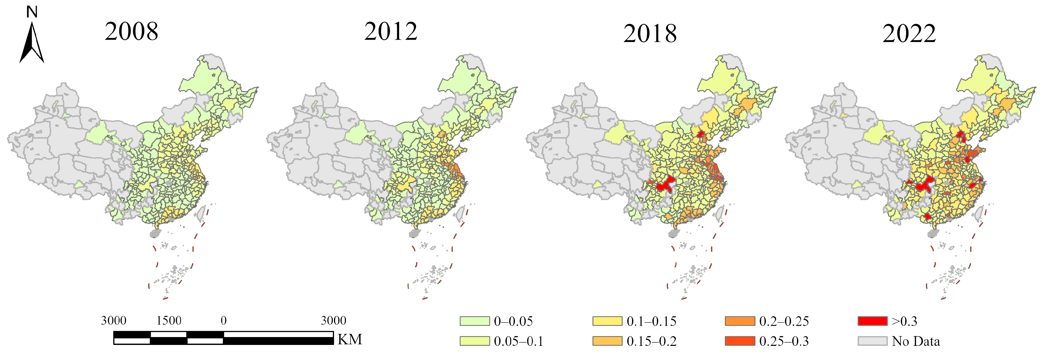
Figure 4 shows the RII levels of prefecture-level cities in different years. Overall, the regions with faster RII growth are mainly coastal cities and important cities such as provincial capitals, while the growth of prefecture-level cities in central and western China is slightly slower.

4.2.3. Mediating Variables

The mediating variables are primarily rural labor transfer (RLT), agricultural technological innovation (ATI), and agricultural carbon emissions (ACE). Rural labor transfer is measured by the proportion of rural non-agricultural employment. Increased non-agricultural employment can increase farmers’ income, thereby promoting the investment of machinery and fertilizers in rural production [40,41], and, to some extent, reflects the flow of rural factors. Agricultural technological innovation can directly improve agricultural production efficiency [57], and the number of adopted patent inventions can reflect the intensity of innovation. Therefore, we use the number of agricultural patent authorizations (in thousands) to measure agricultural technological innovation. RII can internalize the negative environmental externalities in the agricultural production process, which mainly include pollutant and greenhouse gas emissions, and we convert them into agricultural carbon emissions (in million tons) to measure this externality.

4.2.4. Control Variables

This study controls for the following factors affecting AEE: (1) Agricultural Structure (AS): the share of agriculture in broad agricultural output; (2) share of secondary and tertiary industries in GDP; (3) (lnGDP): log of per capita GDP; (4) Urbanization Rate (UR): urban population share; (5) Agricultural Expenditure (AE); the ratio of agriculture-related spending to total fiscal expenditure; (6) Education Expenditure (EE): the share of education spending; (7) Urban–Rural Income Ratio (URIR); (8) (lnRI): the log of rural per capita income; (9) Transportation Level (TL); road mileage. The descriptions of all variables are shown in

Table 3. Variable description.

Variable	Name	Mean	Std. Dev.	Calculation Method
Explained Variable	AEE	0.241	0.081	As shown in Equations (6) and (7)
Key Explanatory Variable	RII	0.086	0.058	Entropy-weighted TOPSIS method
Mediating Variables	RLT	0.387	0.174	Rural non-agricultural employees/Rural employees
	ATI	0.030	0.075	Number of agricultural patent inventions authorized (thousands)
	ACE	0.440	0.336	Agricultural carbon emissions (million tons)
Control Variables	AS	0.526	0.135	Gross output value of agriculture/Gross output value of broadly defined agriculture
	GDP2	0.459	0.112	Value-added of secondary industry/GDP
	GDP3	0.415	0.103	Value-added of tertiary industry/GDP
	lnGDP	10.636	0.659	Log of GDP per capita
	UR	0.545	0.159	Urban permanent population/Total population
	AE	0.120	0.046	Agriculture, Forestry, and Water expenditure/Local government expenditure
	EE	0.178	0.043	Education expenditure/Local government expenditure
	URIR	2.439	0.599	Per capita income of urban residents/Per capita income of rural residents
	lnRI	9.307	0.566	Log of per capita income of rural residents
	TL	1.333	1.058	Highway mileage (10,000 km)

.

4.3. Data Sources

This study uses a balanced panel of 285 Chinese prefecture-level cities from 2008 to 2022. Macroeconomic data are drawn from the EPS database; data on cooperatives and enterprises from the CCAD database; and the list of “Beautiful Leisure Villages” from the Ministry of Agriculture and Rural Affairs (www.moa.gov.cn). Data on the number of authorized agricultural patent inventions are filtered from patents authorized by the National Intellectual Property Administration according to the IPC classification number A01. Some variables are deflated, and missing values are linearly interpolated.

5. Results and Discussion

5.1. Baseline Regression

In

Table 4. Regression results of RII on AEE.

Variable	(1)	(2)	(3)	(4)
RII	0.776 ***	0.526 ***	0.440 **	0.366 ***
	(26.015)	(21.404)	(2.432)	(3.681)
AS		−0.156 ***		−0.082 ***
		(−17.956)		(−5.090)
GDP2		−0.353 ***		−0.204 ***
		(−15.105)		(−3.156)
GDP3		−0.329 ***		−0.297 ***
		(−14.606)		(−4.619)
lnGDP		0.051 ***		0.034 ***
		(9.435)		(2.992)
UR		−0.030 ***		−0.014
		(−2.974)		(−0.783)
AE		−0.374 ***		−0.123 ***
		(−13.178)		(−2.868)
EE		0.243 ***		0.083 **
		(8.106)		(2.133)
URIR		0.005 **		0.008 *
		(2.471)		(1.846)
lnRI		0.004		−0.013
		(0.762)		(−0.708)
TL		0.012 ***		0.023
		(5.693)		(1.148)
Constant	0.174 ***	−0.013	0.185 ***	0.156
	(74.929)	(−0.419)	(17.629)	(1.249)
Year fixed effects	No	No	Yes	Yes
City fixed effects	No	No	Yes	Yes
R2	0.3097	0.4796	0.3664	0.4263

Note: (1) ***, **, * denote significant at the level of 1%, 5%, 10%.

, Models (1) and (2) are OLS regressions without individual and time fixed effects. The coefficients of RII are both positive at the 1% significance level, indicating that RII has a significant promoting effect on AEE. After adding individual and time fixed effects to models (3) and (4), the RII coefficients are both smaller than the OLS regression results, but are still positive at the 1% significance level, the coefficient of RII in model (4) is 0.366, indicating that RII will promote AEE after considering individual and time differences, which verifies Hypothesis 1. After adding control variables, the coefficients of RII in (2) and (4) become smaller, indicating that not adding control variables will lead to an overestimation of the promoting effect of RII on AEE, and other factors can also have an impact on AEE.

5.2. Robustness Analysis

5.2.1. Robustness Tests

Although the baseline regression results indicate a positive effect of RII on AEE, the robustness of these findings requires further validation. As shown in

Table 5. Robustness test results.

Variable	(1)	(2)	(3)	(4)	(5)
RII	0.293 ***	0.734 ***	0.205 ***	0.279 **	0.174 ***
	(3.242)	(3.864)	(3.211)	(2.433)	(3.112)
Constant	−0.032	0.159	−0.055	0.161	0.071
	(−0.273)	(1.201)	(−0.570)	(1.151)	(0.657)
Control	YES	YES	YES	YES	YES
Year fixed effects	YES	YES	YES	YES	YES
City fixed effects	YES	YES	YES	YES	YES
R2	0.4245	0.4096	0.5041	0.3224	0.3849
N	4275	4275	4275	2850	4215

Note: (1) ***, ** denote significant at the level of 1% and 5%.

, Model (1) replaces the dependent variable by recalculating AEE using value added of primary industry instead of gross output of broadly defined agriculture. Model (2) changes the measurement method of key explanatory variables and recalculates the RII using the average weighted TOPSIS method. Model (3) performs a 1% Winsorization on all continuous variables to reduce the impact of outliers. Model (4) changes the time range of the sample. Because some variables have missing values in the early years during the data acquisition process, the sample after 2012 is re-regressed. Model (5) alters the sample by eliminating municipalities—Beijing, Tianjin, Shanghai, and Chongqing—given their unique administrative status and potentially different scales of agricultural development. In all models, RII coefficients are positive and significant, this confirms the robustness of RII’s positive effect on AEE and further supports Hypothesis 1.

5.2.2. Endogeneity Test

The effect of RII on AEE may be subject to estimation bias due to potential endogeneity issues such as omitted variables or reverse causality, so we consider using the instrumental variables (IV) method to address potential endogeneity. RII reflects the level of rural industrialization development, which is influenced by factors such as natural endowment and economic development. This study uses the number of agricultural-related enterprises (in 10,000) in each prefecture-level city as an instrumental variable. Since agricultural-related enterprises include various types of enterprises such as agricultural production and auxiliary activities, they can reflect market activities related to agriculture in rural areas. Therefore, regions with a large number of agricultural-related enterprises have a higher level of marketization, which promotes exchanges between enterprises in different industries and is positively correlated with the RII. Moreover, agricultural-related enterprises also include many agricultural non-productive enterprises, which reflect market activities in rural areas and do not directly affect agricultural production efficiency, so it can be considered exogenous to AEE. The results of the 2SLS estimation are shown in

Table 6. The results of the endogenous test.

Variable	(1)	(2)
	RII	AEE
IV	0.0339 ***
	(15.71)
RII		0.565 ***
		(6.86)
Control	YES	YES
Year fixed effects	YES	YES
City fixed effects	YES	YES
N	4275	4275
Under-identification test—Kleibergen-Paap rk LM statistic: 60.06 ***. Weak instrument test—Kleibergen-Paap rk Wald F statistic: 246.887. 10% critical value: 16.380.

Note: (1) *** denote significant at the level of 1%.

. Model (1) is the first-stage regression result of the instrumental variables on RII. The coefficient of IV is positive at the 1% significance level, avoiding the problem of weak instrumental variables. Model (2) is the second-stage result of 2SLS. The coefficient of RII is also positive at the 1% significance level, verifying the robustness of the baseline regression. The Kleibergen–Paap rk LM statistic is 60.06, the test rejects the null of under-identification at 1% significance. Kleibergen–Paap rk Wald F-statistic is 246.887, surpassing the 10% critical value of 16.38, indicating instrument is strong. These tests validate the instrument and further support Hypothesis 1.

5.2.3. Policy Impact Analysis

The Chinese government launched the “Hundreds of Counties, Thousands of Towns, and Ten Thousand Villages” pilot demonstration project for RII development in 2016, and selected 137 counties across the country as pilot demonstration areas for RII development. The pilot areas accelerated the development of industrial integration, and the RII also reached a leading level. To include the impact of RII policy shocks on AEE, this study uses a quasi-natural experiment approach, using prefecture-level cities where the national rural industrial integration development pilot demonstration counties are located as the experimental group and other prefecture-level cities without pilot demonstration counties as the control group. Taking the announcement of the pilot in 2016 as the time point of policy impact, a difference-in-differences (DID) approach is used to examine the impact of RII policies on AEE. The specific econometric model is as follows:

$${\mathrm{A}\mathrm{E}\mathrm{E}}_{\mathrm{i}\mathrm{t}}={\mathrm{c}}_0+{\mathrm{c}}_1{\mathrm{T}reat}_{\mathrm{i}\mathrm{t}}+{\mathrm{c}}_2{\mathrm{X}}_{\mathrm{i}\mathrm{t}}+{\mathsf{\mu }}_{\mathrm{i}}+{\mathsf{\delta }}_{\mathrm{t}}+{\mathsf{\epsilon }}_{\mathrm{i}\mathrm{t}}$$

(9)

${\mathrm{A}\mathrm{E}\mathrm{E}}_{\mathrm{i}\mathrm{t}}$ denotes agriculture eco-efficiency, ${\mathrm{T}reat}_{\mathrm{i}\mathrm{t}}$ represents a policy dummy variable, indicating whether region $\mathrm{i}$ is affected by policy shocks at time $\mathrm{t}$, and ${\mathrm{X}}_{\mathrm{i}\mathrm{t}}$ includes various control variables, $\mathrm{c}$ is the estimated coefficients, ${\mathsf{\mu }}_{\mathrm{i}}{\mathsf{\delta }}_{\mathrm{t}}{\mathsf{\epsilon }}_{\mathrm{i}\mathrm{t}}$ are fixed effects and disturbance terms.

Before conducting the regression, we need to ensure that there is a parallel trend in AEE between the experimental group and the control group. From the time trend graphs of the experimental and control groups in Figure 5, it can be observed that before the policy shock, both groups maintained the same growth trend in AEE. However, starting from the year the pilot policy was implemented, the gap in AEE between the experimental and control groups began to widen, which aligns with the assumption of a parallel trend.

In

Table 7. The effect of RII development pilot policy.

Variable	(1)	(2)
Treat	0.023 ***	0.020 ***
	(3.179)	(3.453)
AS		−0.078 ***
		(−4.690)
GDP2		−0.170 **
		(−2.542)
GDP3		−0.249 ***
		(−3.837)
lnGDP		0.036 ***
		(2.821)
UR		−0.026
		(−1.214)
AE		−0.121 ***
		(−2.648)
EE		0.101 **
		(2.587)
URIR		0.006
		(1.334)
lnRI		−0.029
		(−1.503)
TL		0.035
		(1.291)
Constant	0.209 ***	0.256 *
	(103.934)	(1.863)
Year fixed effects	YES	YES
City fixed effects	YES	YES
R2	0.3042	0.3919
N	4275	4275

Note: (1) ***, **, * denote significant at the level of 1%, 5%, 10%.

, Model (1) shows the results of DID without adding control variables. The coefficient of the policy variable treat is 0.023, passing the 1% significance level test. Model (2) adds a series of control variables from the baseline regression model. The coefficient of treat is 0.02, which is still positive at the 1% significance level, indicating that the AEE level of the experimental group is 0.02 higher than that of the control group. This shows that after the implementation of the RII policy in the pilot areas, AEE has increased significantly, further verifying Hypothesis 1. It also indicates that the Chinese government’s proactive promotion of RII practice can effectively promote sustainable agricultural development.

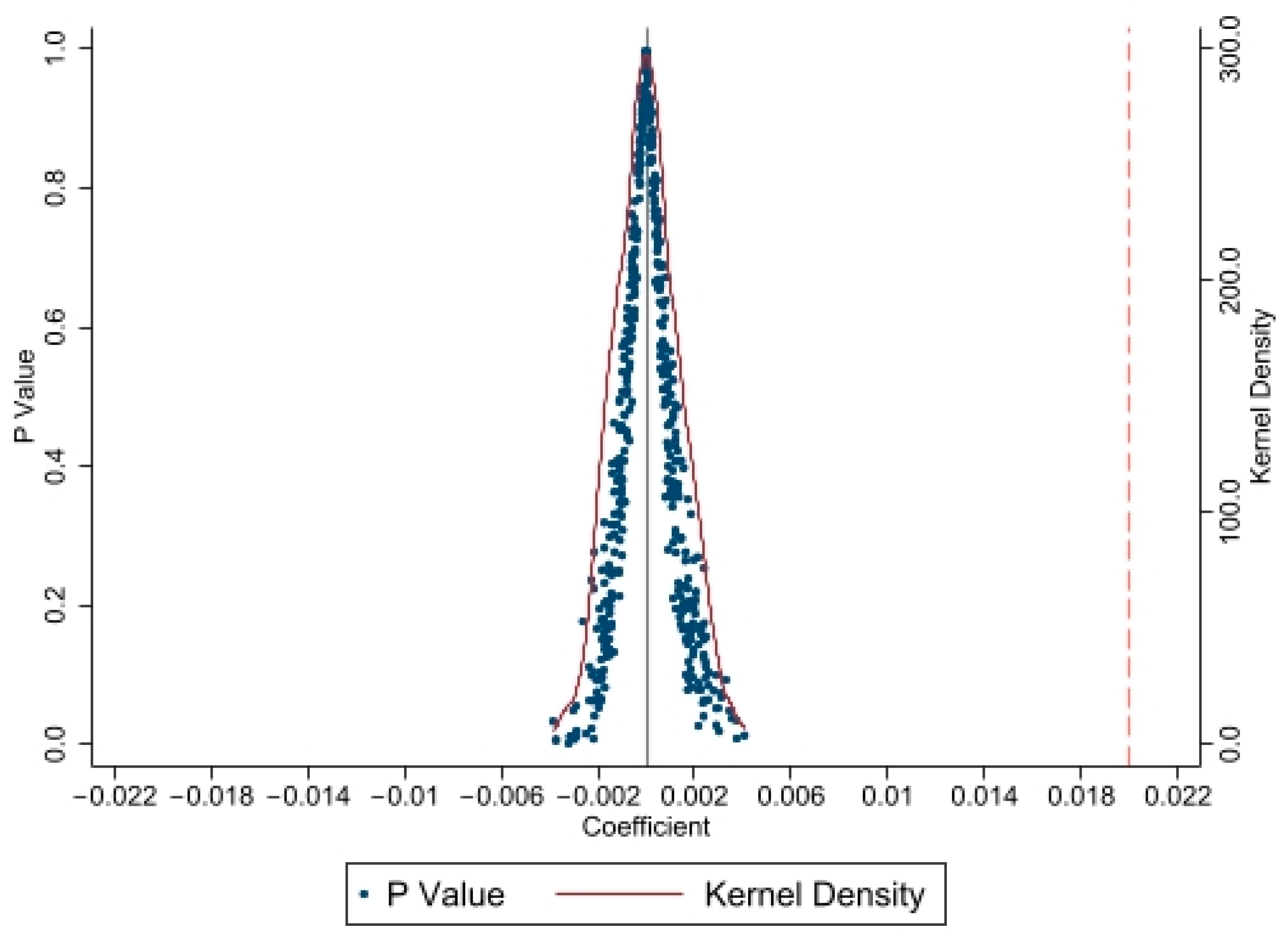
The impact of the pilot policy on AEE may also be affected by random factors. To ensure the robustness of the findings, this paper conducts an indirect placebo test. Specifically, the treatment group was randomly reassigned to the RII pilot program and time to generate erroneous estimates of the DID coefficient. This procedure was repeated 500 times, and the distribution of the resulting coefficients was examined. As shown in Figure 6, these estimated coefficients are distributed around 0, deviating from the actual regression coefficient of 0.02, and approximately follow a normal distribution, suggesting that unobserved factors do not exert a significant influence on the results, further ensuring the robustness of the DID regression results.

5.3. Mechanism Analysis

Table 8. Mechanism test.

Variable	(1)	(2)	(3)	(4)	(5)	(6)
	RLT	ATI	ACE	AEE	AEE	AEE
RII	0.313 ***	0.138 ***	−0.258 ***	0.355 ***	0.357 ***	0.329 ***
	(3.690)	(3.074)	(−4.088)	(3.534)	(3.555)	(3.451)
RLT				0.033 **
				(2.558)
ATI					0.063 **
					(2.166)
ACE						−0.142 ***
						(−5.523)
Constant	−1.393 ***	−0.031	0.129	0.201	0.158	0.174
	(−3.667)	(−0.238)	(0.615)	(1.561)	(1.263)	(1.395)
Control	YES	YES	YES	YES	YES	YES
Year fixed effects	YES	YES	YES	YES	YES	YES
City fixed effects	YES	YES	YES	YES	YES	YES
R2	0.1098	0.1921	0.1666	0.4299	0.4290	0.4543
N	4275	4275	4275	4275	4275	4275

Note: (1) ***, ** denote significant at the level of 1% and 5%.

shows the results of the mechanism analysis. Models (1), (2), and (3) are regressions of RII on mediating variables. The regression coefficient of RII on LRT is 0.313, which passed the 1% significance level test, indicating that RII can significantly promote labor transfer. The regression coefficient of RII on ATI is 0.138, which also passed the 1% significance level test, indicating that RII helps promote agricultural technological innovation. The regression coefficient of RII on ACE is −0.258, which is negative at the 1% significance level, indicating that RII development will inhibit agricultural carbon emissions. Models (4), (5), and (6) are regressions of AEE after adding mediating variables. The coefficient of LRT is 0.033, and the coefficient of ATI is 0.063, both of which passed the 5% significance level test, indicating that both can promote the improvement of AEE. The coefficient of ACE is −0.142, which is negative at the 1% significance level, indicating that excessive agricultural carbon emissions are not conducive to the improvement of AEE.

Mechanism testing results indicate that RII improves AEE by promoting labor transfer, enhancing agricultural technological innovation, and reducing agricultural carbon emissions. RII develops the rural non-agricultural sector, creating more employment opportunities and thus leading to labor transfer. Increased rural non-agricultural employment promotes land transfer, while also increasing farmers’ incomes. This leads some agricultural operators to invest more in agriculture. Therefore, labor transfer reflects the flow of factors between the agricultural and non-agricultural sectors in rural areas, promoting AEE, which confirms Hypothesis 2. RII integrates different industries and fosters technological exchange between them, thereby enhancing agricultural technological innovation. The technological integration brought about by RII directly promotes technological progress in agricultural production, thereby improving AEE, which confirms Hypothesis 3. Since agricultural product processing and rural tourism avoid the negative environmental externalities of agricultural production, and RII development aims to maximize shared benefits, these externalities are effectively internalized, thereby reducing agricultural carbon emissions. Reduced carbon emissions also directly promote AEE, confirming Hypothesis 4.

5.4. Spatial Effects Analysis

To evaluate the spatial impact of RII on AEE, this study first tests for spatial autocorrelation using Moran’s I statistic with a geographic distance-based spatial weight matrix to assess annual spatial dependencies. Global Moran’s I coefficients for both RII and AEE are statistically significant at 1% level in

Table 9. Spatial autocorrelation Moran index.

Year	RII		AEE
	I	Z	I	Z
2008	0.1675 ***	33.4978	0.1124 ***	22.9045
2009	0.1641 ***	32.8583	0.1053 ***	21.5118
2010	0.1659 ***	33.2141	0.0966 ***	19.7891
2011	0.1633 ***	32.7051	0.0941 ***	19.2815
2012	0.1651 ***	33.0594	0.0902 ***	18.5624
2013	0.1606 ***	32.1548	0.0866 ***	17.8579
2014	0.1558 ***	31.2255	0.0889 ***	18.3385
2015	0.152 ***	30.482	0.0919 ***	18.9687
2016	0.1395 ***	28.0607	0.0777 ***	16.1497
2017	0.1295 ***	26.1188	0.0889 ***	18.4522
2018	0.118 ***	23.898	0.0847 ***	17.6861
2019	0.1054 ***	21.5339	0.078 ***	16.3953
2020	0.0929 ***	19.1461	0.0647 ***	13.8414
2021	0.0352 ***	7.858	0.0648 ***	13.8117
2022	0.0323 ***	7.2434	0.0536 ***	11.5506

Note: (1) *** denote significant at the level of 1%.

, confirming notable spatial autocorrelation. Consequently, the use of spatial econometric methods is warranted to appropriately model these spatial effects.

Before conducting empirical analysis using spatial econometric models, a series of diagnostic tests—including LM test, LR test, Wald test, and Hausman test—must be performed to determine the appropriate model specification. As presented in

Table 10. Spatial model test results.

Spatial Model Test	Statistics
LM (error)	750.408 ***
Robust LM (error)	589.586 ***
LM (lag)	171.576 ***
Robust LM (lag)	10.755 ***
LR (lag)	147.03 ***
LR (error)	118.93 ***
Wald (lag)	141.05 ***
Wald (error)	107.61 ***
Hausman test	73.28 ***
Individual LR test	49.81 ***
Time LR test	5509.12 ***

Note: (1) *** denote significant at the level of 1%.

, all test results are significant at the 1% level. Findings indicate the necessity to consider spatial lag and error effects, justifying the adoption of a two-way fixed effects model.

In

Table 11. Spatial model regression results.

Variable	W1			W2	W3
	(1)	(2)	(3)	(4)	(5)
	SLM	SEM	SDM	SDM	SDM
RII	0.355 ***	0.379 ***	0.399 ***	0.428 ***	0.331 ***
	(18.819)	(19.422)	(19.501)	(20.756)	(17.241)
W*RII			−2.359 ***	−0.313 ***	0.317 ***
			(−5.060)	(−9.519)	(4.765)
ρ or λ	2.124 ***	2.062 ***	1.803 ***	0.275 ***	0.003
	(23.344)	(19.509)	(10.600)	(13.602)	(0.095)
Control Variables	Yes	Yes	Yes	Yes	Yes
Year fixed effects	Yes	Yes	Yes	Yes	Yes
City fixed effects	Yes	Yes	Yes	Yes	Yes
R2	0.2794	0.2357	0.2674	0.0001	0.1023
N	4275	4275	4275	4275	4275

Note: (1) *** denote significant at the level of 1%.

, Models (1), (2), (3) report regression results based on the geographical distance matrix (W1). The spatial autocorrelation coefficients or spatial error coefficients are significant and positive, indicating the existence of positive spatial effects. In all three models—SLM, SEM, and SDM—RII coefficients are significantly positive at the 1% level, suggesting that RII continues to exert a positive effect on AEE under spatial model specifications. In model (3), the coefficient of the spatial lag term of RII is negative at the 1% significance level, which indicates that RII may inhibit the improvement of AEE in neighboring regions. However, the spillover effect of RII on AEE cannot be judged based on this. Further decomposition of the spatial effect is needed to draw a conclusion. Additionally, Models (4) and (5) present the SDM results using contiguity matrix (W2) and economic distance matrix (W3). The estimated coefficients of RII remain consistent with those under W1; however, the R² of W2 is too small, and the spatial autocorrelation coefficient under W3 is not statistically significant. Thus, the regression results based on W1 are considered the most robust.

Due to spatial lag of AEE, decomposing the effects is required to isolate the true direct influence and spatial spillover effects of RII on AEE. The SLM and SDM models were used to decompose direct, spillover, and total effects RII exerts on AEE, as presented in

Table 12. Spatial effect decomposition.

Variable	(1)	(2)	(3)
	Direct Effect	Spillover Effect	Total Effect
SLM:
RII	0.363 ***	2.108	2.471 *
	(18.116)	(1.641)	(1.916)
SDM:
RII	0.391 ***	−2.280 **	−1.889 *
	(18.948)	(−2.283)	(−1.891)

Note: (1) ***, **, * denote significant at the level of 1%, 5%, 10%.

. The results show that the direct effect of RII on AEE is positive at the 1% significance level in both the SLM and SDM models, indicating that RII promotes AEE in the local region, consistent with Hypothesis 1. In the SLM model, the spillover effect is positive but not significant, while in the SDM model, it is negative at the 5% significance level, indicating that RII increases AEE in neighboring regions. This phenomenon of suppressing AEE in other regions while promoting AEE in the local region demonstrates the characteristics of a “siphon effect”. The existence of the “siphon effect” may be due to the competition for various resources in the development process of RII in different regions. Since resource factors can flow between regions, areas with higher AEE can obtain more output returns, thereby attracting factors such as labor and capital, which in turn negatively affects other regions’ AEE. These effects cross geographical boundaries, thereby having a spillover effect on AEE, verifying Hypothesis 5.

5.5. Heterogeneity Analysis

5.5.1. Regional Heterogeneity

This study analyzes the differences in the impact of RII on AEE through regional heterogeneity. All prefecture-level cities are divided into four major regions: east, mid, west, and northeast; the results of SDM group regression are shown in

Table 13. SDM regression results by region.

Variable	(1)	(2)	(3)	(4)
	East	Mid	West	Northeast
RII	0.250 ***	0.392 ***	0.675 ***	0.215 ***
	(6.374)	(11.072)	(17.313)	(4.101)
W*RII	−1.641 *	5.576 ***	5.526 **	1.607
	(−1.652)	(4.052)	(2.125)	(0.970)
Direct effect	0.253 ***	0.436 ***	0.675 ***	0.218 ***
	(6.191)	(10.547)	(16.969)	(4.046)
Spillover effect	−0.279 *	3.905 ***	0.663 *	0.185
	(−1.804)	(2.804)	(1.795)	(0.988)
Total effect	−0.026	4.341 ***	1.338 ***	0.403 **
	(−0.187)	(3.071)	(3.538)	(2.327)
Control Variables	Yes	Yes	Yes	Yes
R2	0.3651	0.4928	0.4829	0.0284
Cities	85	80	86	34
Observes	1275	1200	1290	510

Note: (1) ***, **, * denote significant at the level of 1%, 5%, 10%.

. The coefficients of RII are significantly positive across all regions, indicating that RII contributes to improvements in AEE nationwide. This suggests that the promotion of industrial integration can positively influence AEE regardless of regional disparities, supporting the notion that China’s industrial integration practices can overcome geographic differences and facilitate synergistic development of industrialization and sustainable agriculture. According to the results of the spatial effect decomposition, the direct effects are significantly positive across all regions, indicating that local RII development consistently promotes improvements in local AEE. Compared with other regions, the coefficient of the direct effect is larger in the western region, indicating that RII has a stronger impact on improving local AEE in less developed regions. This suggests that the resource flows brought about by RII can more effectively alleviate the obstacles caused by resource inequality and stimulate sustainable agricultural development. However, the spillover effects exhibit marked regional disparities. The spillover effect coefficient of the eastern region is −0.279, which is negative at the 10% significance level, showing a “siphon effect”, suggesting that the development of local RII hinders the improvement of AEE in other regions. This may be due to the more developed economy in the eastern regions, leading to smaller development gaps between regions and thus less significant differences in factor endowments. As a result, the development of RII in different regions is more substitutive than complementary. The development of RII siphons various resources and factors from other regions, thereby hindering the improvement of AEE in other areas. Conversely, the spillover effect is positive in mid and west, while the spillover effect in the northeast is not significant. The spatial spillover effect coefficient in mid is 3.905, significantly positive, showing RII can drive the improvement of AEE in other areas. Due to the larger development disparities in the central region, some developed areas have higher capital and technology levels, while less developed areas have more abundant labor and land factors, making the flow of complementary factors and technology integration between regions easier to occur. The spatial spillover coefficient in west is 0.663, only positive at the 10% significance level. This may be because although there is a trend of factor mobility and technology dissemination in the western region, which is constrained by poor infrastructure, making it difficult for the spillover effect of RII to take effect. The coefficient of spillover effects in the northeast region is 0.185 but not significant, indicating that the spillover effect is not prominent.

5.5.2. RII Development Model Heterogeneity

From the perspective of integration direction, industrial integration can be divided into vertical integration and horizontal integration. Vertical integration primarily refers to the vertical integration of the industrial chain, while horizontal integration occurs around the multifunctionality of the industry [34]. This can correspond to the integration between agriculture and the agricultural product processing industry (first and second industries) and the integration between agriculture and the service and tourism industry (first and third industries). To account for the differences in the impact of various integration modes on AEE, we have categorized RII to analyze the heterogeneity of different development models. We use the coupling coordination degree (CCD) model to measure the degree of integration between the primary and secondary industries or the primary and tertiary industries [58], and distinguish the differences in development patterns among regions by comparing the two coupling degrees. The specific approach is that we use the RII index system’s industrial chain extension as a measure of the development of the secondary industry, multi-functional expansion and service integration as a measure of the development of the tertiary industry, and technology penetration as a measure of the development of the primary industry. Then, we use the results of the primary and secondary industries or the primary and tertiary industries to calculate the CCD. Finally, generate virtual variables D12 and D13 for these two industrial integration models based on the relative size of the CCD.

We added the moderating model of RII interacting with two virtual variables as shown in

Table 14. Heterogeneity of development models.

Variable	(1)	(2)
RII*D12	0.242 ***	0.308 ***
	(2.694)	(11.945)
RII*D13	0.364 ***	0.395 ***
	(3.766)	(19.354)
W*RII*D12		−2.030 ***
		(−3.810)
W*RII*D13		−2.161 ***
		(−4.550)
Control Variables	Yes	Yes
Year fixed effects	Yes	Yes
City fixed effects	Yes	Yes
R2	0.4356	0.2941
N	4275	4275

Note: (1) *** denote significant at the level of 1%.

. Among them, (1) is the fixed effects model, where the coefficient of RII*D12 is 0.242 and the coefficient of RII*D13 is 0.364, both positive at the 1% significance level, indicating that RII can promote the improvement of AEE whether in the integration mode of the primary and secondary industries or the primary and tertiary industries. In contrast, the coefficient of RII*D13 is larger, suggesting that RII has a stronger promoting effect on AEE under the integration of the primary and tertiary industries. Model (2) is the regression results of the SDM, where the coefficients remain significant, indicating that the above relationship still exists when considering spatial effects. The above analysis reveals that the integration of the primary and tertiary industries is more conducive to increasing AEE. This may be due to the wider scope of integration between the service, tourism, and agricultural sectors. The development of various leisure farms or rural tourism benefits more farmers, who are more likely to prioritize environmental protection. The ecological benefits of environmental protection also directly benefit them, thereby achieving sustainable agricultural development.

6. Conclusions and Implications

6.1. Conclusions

The pursuit of rural industrialization and sustainable agricultural development lies in achieving both farmers’ prosperity and meeting broader societal needs, while China’s RII practice has promoted the coordinated advancement of these two goals. RII has already achieved great results in promoting rural industrial development in the rural revitalization program, and our research focuses on the potential impact of RII on agricultural sustainability. By verifying the promoting effect of RII on AEE, we demonstrate that advancing RII can simultaneously achieve rural industrialization and agricultural sustainable development. This study uses a 2008–2022 panel of 285 prefecture-level cities in China to measure AEE with a super-efficiency SBM model, constructs a comprehensive index system for RII, empirically test the impact and spillover effects of RII on AEE using panel fixed effect models and spatial econometric models, and adopts the mediation effect model to analyze the specific mechanism. Results indicate RII significantly enhances AEE, and the findings still hold under various robustness tests and instrumental variable regressions. By analyzing the impact of policy shocks, we find that after the Chinese government implemented RII support policies, AEE increased significantly. In addition, the impact of RII on AEE also has a spatial spillover effect, and presents the characteristics of the “siphon effect”. The results of regional heterogeneity show that the spillover effect in the eastern region is negative, the central and western regions have positive spillover effects, and the spillover effect in the northeastern region is not significant. Considering the heterogeneity of the industrial integration model, RII has a stronger promotion effect on AEE under the development model dominated by the integration of primary and tertiary industries.

6.2. Implications

Promoting RII development can effectively enhance AEE, which is of significant importance to advancing rural industrialization and sustainable agricultural development. RII not only directly promotes the development of non-agricultural industries in rural areas, but also enhances AEE, thereby synergizing agricultural sustainability with rural industrialization and achieving their common development. These findings offer valuable insights for regions facing underdeveloped rural, low agricultural productivity, and severe environmental pollution. From the RII practice in China, this study puts forward the following policy implications for rural industrialization and agricultural sustainable development.

First, since RII can significantly promote the improvement of AEE, some regions can leverage the comparative advantages of agriculture and rural resources during the industrialization of rural areas, promote the flow of production factors between the primary, secondary, and tertiary industries, and enable integrated development among these industries to maximize overall economic benefits. Policymakers can implement pilot policies in selected regions, leveraging the demonstration effect of regions with RII potential to promote overall RII development.

Second, since RII has a mediating effect on AEE, in the process of advancing RII development it is necessary to maintain market stability and promote the normal flow of factors, encourage technological innovation and promote technological exchange to improve technological levels, aim at maximizing common interests, and encourage the adoption of green agricultural technologies to reduce the impact of environmental externalities.

Third, because RII’s impact on AEE has spillover effects, exhibiting a “siphon effect,” it is necessary to avoid negative spatial externalities between regions. Different regions should reduce unnecessary competition for resource factors, develop complementary industries, and enhance technological innovation to boost AEE.

Fourth, considering the heterogeneity of regions, differentiated policies should be implemented based on the relative advantages of regional resources and resource distribution. For the eastern regions, it is necessary to avoid adverse spatial externalities generated during the development of RII, focus on technological innovation, reduce reliance on resources, and thereby avoid unnecessary competition. The development gaps between central and western regions are significant, and resource factors in different regions can complement each other to some extent, so regional exchanges and mutual connectivity should be encouraged. In the northeastern region, the promoting effect of RII on AEE is relatively weak, and the spillover effect is also not strong, so during the development process, it is necessary to identify the relative advantages of its own industries and steadily promote AEE growth.

Fifth, different RII development models have varying effects on AEE. The integration of primary and tertiary industries is more effective in promoting AEE. Therefore, for regions with a certain level of RII development, a transition to a more advanced development model is an appropriate option. However, regions undergoing this transition should also consider their own resource constraints; blindly pursuing advanced industries is unsustainable.

This study obtained some valuable new findings on the impact of RII on AEE, but it also has certain limitations. Due to data availability, some prefecture-level cities in the western region were not within the sample. Future research will utilize larger sample sizes to generate more realistic results.

References

1. Alexander, P.; Rounsevell, M.D.A.; Dislich, C.; Dodson, J.R.; Engström, K.; Moran, D. Drivers for global agricultural land use change: The nexus of diet, population, yield and bioenergy. Glob. Environ. Change 2015, 35, 138–147. [Google Scholar] [CrossRef]
2. Johnson, J.A.; Runge, C.F.; Senauer, B.; Foley, J.; Polasky, S. Global agriculture and carbon trade-offs. Proc. Natl. Acad. Sci. USA 2014, 111, 12342–12347. [Google Scholar] [CrossRef] [PubMed]
3. Zhang, Q.; Qu, Y.; Zhan, L. Great transition and new pattern: Agriculture and rural area green development and its coordinated relationship with economic growth in China. J. Environ. Manag. 2023, 344, 118563. [Google Scholar] [CrossRef] [PubMed]
4. Streimikis, J.; Baležentis, T. Agricultural sustainability assessment framework integrating sustainable development goals and interlinked priorities of environmental, climate and agriculture policies. Sustain. Dev. 2020, 28, 1702–1712. [Google Scholar] [CrossRef]
5. Hickel, J. The sustainable development index: Measuring the ecological efficiency of human development in the anthropocene. Ecol. Econ. 2020, 167, 106331. [Google Scholar] [CrossRef]
6. Struik, P.C.; Kuyper, T.W. Sustainable intensification in agriculture: The richer shade of green. A review. Agron. Sustain. Dev. 2017, 37, 39. [Google Scholar] [CrossRef]
7. Liu, Y.; Huang, J.; Zikhali, P. The bittersweet fruits of industrialization in rural China: The cost of environment and the benefit from off-farm employment. China Econ. Rev. 2016, 38, 1–10. [Google Scholar] [CrossRef]
8. Xu, Y.; Li, H.; Zhang, R.; Wang, T.; Sui, P.; Sheng, J.; Gao, W.; Chen, Y. Balancing the development and carbon emissions in rural areas of China. J. Clean. Prod. 2024, 454, 142338. [Google Scholar] [CrossRef]
9. Zhou, L.; Li, Y.Y.; Wang, C.H.; Fang, P. Development of industrial integration and sixth industry in rural vitalization strategy. J. Xinjiang Norm. Univ. (Ed. Philos. Soc. Sci.) 2018, 39, 16–24. (In Chinese) [Google Scholar]
10. Ma, L.; Liu, S.; Fang, F.; Che, X.; Chen, M. Evaluation of urban-rural difference and integration based on quality of life. Sust. Cities Soc. 2020, 54, 101877. [Google Scholar] [CrossRef]
11. Xiao, W.; Du, Z. Integration of rural primary, secondary and tertiary industries: Kernel interpretation of connotation, development status and future ideas. J. Northwest A&F Univ. 2019, 19, 120–129. [Google Scholar]
12. Tian, X.; Wu, M.; Ma, L.; Wang, N. Rural finance, scale management and rural industrial integration. China Agric. Econ. Rev. 2020, 12, 349–365. [Google Scholar] [CrossRef]
13. Müller, K.; Holmes, A.; Deurer, M.; Clothier, B.E. Eco-efficiency as a sustainability measure for kiwifruit production in New Zealand. J. Clean. Prod. 2015, 106, 333–342. [Google Scholar] [CrossRef]
14. Caiado, R.G.G.; de Freitas Dias, R.; Mattos, L.V.; Quelhas, O.L.G.; Leal Filho, W. Towards sustainable development through the perspective of eco-efficiency—A systematic literature review. J. Clean. Prod. 2017, 165, 890–904. [Google Scholar] [CrossRef]
15. Liao, J.; Yu, C.; Feng, Z.; Zhao, H.; Wu, K.; Ma, X. Spatial differentiation characteristics and driving factors of agricultural eco-efficiency in Chinese provinces from the perspective of ecosystem services. J. Clean. Prod. 2021, 288, 125466. [Google Scholar] [CrossRef]
16. Coluccia, B.; Valente, D.; Fusco, G.; De Leo, F.; Porrini, D. Assessing agricultural eco-efficiency in Italian Regions. Ecol. Indic. 2020, 116, 106483. [Google Scholar] [CrossRef]
17. Orea, L.; Wall, A. A Parametric Approach to Estimating Eco-Efficiency. J. Agric. Econ. 2017, 68, 901–907. [Google Scholar] [CrossRef]
18. Liu, Y.; Zou, L.; Wang, Y. Spatial-temporal characteristics and influencing factors of agricultural eco-efficiency in China in recent 40 years. Land Use Policy 2020, 97, 104794. [Google Scholar] [CrossRef]
19. Yang, H.; Wang, X.; Bin, P. Agriculture carbon-emission reduction and changing factors behind agricultural eco-efficiency growth in China. J. Clean. Prod. 2022, 334, 130193. [Google Scholar] [CrossRef]
20. Grassauer, F.; Herndl, M.; Nemecek, T.; Guggenberger, T.; Fritz, C.; Steinwidder, A.; Zollitsch, W. Eco-efficiency of farms considering multiple functions of agriculture: Concept and results from Austrian farms. J. Clean. Prod. 2021, 297, 126662. [Google Scholar] [CrossRef]
21. Deng, X.; Gibson, J. Improving eco-efficiency for the sustainable agricultural production: A case study in Shandong, China. Technol. Forecast. Soc. Change 2019, 144, 394–400. [Google Scholar] [CrossRef]
22. Czyżewski, B.; Matuszczak, A.; Grzelak, A.; Guth, M.; Majchrzak, A. Environmental sustainable value in agriculture revisited: How does Common Agricultural Policy contribute to eco-efficiency? Sustain. Sci. 2021, 16, 137–152. [Google Scholar] [CrossRef]
23. Grzelak, A.; Guth, M.; Matuszczak, A.; Czyżewski, B.; Brelik, A. Approaching the environmental sustainable value in agriculture: How factor endowments foster the eco-efficiency. J. Clean. Prod. 2019, 241, 118304. [Google Scholar] [CrossRef]
24. Ait Sidhoum, A.; Canessa, C.; Sauer, J. Effects of agri-environment schemes on farm-level eco-efficiency measures: Empirical evidence from EU countries. J. Agric. Econ. 2023, 74, 551–569. [Google Scholar] [CrossRef]
25. Wu, K.; You, K.; Ren, H.; Gan, L. The impact of industrial agglomeration on ecological efficiency: An empirical analysis based on 244 Chinese cities. Environ. Impact Assess. Rev. 2022, 96, 106841. [Google Scholar] [CrossRef]
26. Wang, F.; Wu, M.; Du, X. Does industrial upgrading improve eco-efficiency? Evidence from China’s industrial sector. Energy Econ. 2023, 124, 106774. [Google Scholar] [CrossRef]
27. Baldassarre, B.; Schepers, M.; Bocken, N.; Cuppen, E.; Korevaar, G.; Calabretta, G. Industrial Symbiosis: Towards a design process for eco-industrial clusters by integrating Circular Economy and Industrial Ecology perspectives. J. Clean. Prod. 2019, 216, 446–460. [Google Scholar] [CrossRef]
28. Ding, J.; Liu, B.; Shao, X. Spatial effects of industrial synergistic agglomeration and regional green development efficiency: Evidence from China. Energy Econ. 2022, 112, 106156. [Google Scholar] [CrossRef]
29. Zhou, Y.; Kong, Y.; Sha, J.; Wang, H. The role of industrial structure upgrades in eco-efficiency evolution: Spatial correlation and spillover effects. Sci. Total Environ. 2019, 687, 1327–1336. [Google Scholar] [CrossRef]
30. Long, H.; Zou, J.; Liu, Y. Differentiation of rural development driven by industrialization and urbanization in eastern coastal China. Habitat Int. 2009, 33, 454–462. [Google Scholar] [CrossRef]
31. Li, Y.; Westlund, H.; Liu, Y. Why some rural areas decline while some others not: An overview of rural evolution in the world. J. Rural Stud. 2019, 68, 135–143. [Google Scholar] [CrossRef]
32. Li, Y.; Jia, L.; Wu, W.; Yan, J.; Liu, Y. Urbanization for rural sustainability—Rethinking China’s urbanization strategy. J. Clean. Prod. 2018, 178, 580–586. [Google Scholar] [CrossRef]
33. Han, J. Prioritizing agricultural, rural development and implementing the rural revitalization strategy. China Agric. Econ. Rev. 2020, 12, 14–19. [Google Scholar] [CrossRef]
34. Su, Y.Q.; You, Y.T.; Wang, Z.G. Convergence development of primary, secondary and tertiary industries: Theoretical discussion, situation analysis and suggestions. China Soft Sci. 2016, 308, 17–28. [Google Scholar]
35. Gambardella, A.; Torrisi, S. Does technological convergence imply convergence in markets? Evidence from the electronics industry. Res. Policy 1998, 27, 445–463. [Google Scholar] [CrossRef]
36. Lei, D.T. Industry evolution and competence development: The imperatives of technological convergence. Int. J. Technol. Manag. 2000, 19, 699–738. [Google Scholar] [CrossRef]
37. Farrell, J.; Shapiro, C. Scale economies and synergies in horizontal merger analysis. Antitrust Law J. 2000, 68, 685. [Google Scholar] [CrossRef]
38. Wang, J.; Peng, L.; Chen, J.; Deng, X. Impact of rural industrial integration on farmers’ income: Evidence from agricultural counties in China. J. Asian Econ. 2024, 93, 101761. [Google Scholar] [CrossRef]
39. Zhou, J.; Chen, H.; Bai, Q.; Liu, L.; Li, G.; Shen, Q. Can the Integration of Rural Industries Help Strengthen China’s Agricultural Economic Resilience? Agriculture 2023, 13, 1813. [Google Scholar] [CrossRef]
40. Zhang, Y.; Long, H.; Li, Y.; Ge, D.; Tu, S. How does off-farm work affect chemical fertilizer application? Evidence from China’s mountainous and plain areas. Land Use Policy 2020, 99, 104848. [Google Scholar] [CrossRef]
41. Zheng, H.; Ma, W.; Guo, Y.; Zhou, X. Interactive relationship between non-farm employment and mechanization service expenditure in rural China. China Agric. Econ. Rev. 2022, 14, 84–105. [Google Scholar] [CrossRef]
42. Gong, B. Agricultural reforms and production in China: Changes in provincial production function and productivity in 1978–2015. J. Dev. Econ. 2018, 132, 18–31. [Google Scholar] [CrossRef]
43. Lu, F.; Meng, J.; Cheng, B. How does improving agricultural mechanization affect the green development of agriculture? Evidence from China. J. Clean. Prod. 2024, 472, 143298. [Google Scholar] [CrossRef]
44. Xie, H.; Lu, H. Impact of land fragmentation and non-agricultural labor supply on circulation of agricultural land management rights. Land Use Policy 2017, 68, 355–364. [Google Scholar] [CrossRef]
45. Song, H.; Jiang, H.; Zhang, S.; Luan, J. Land circulation, scale operation, and agricultural carbon reduction efficiency: Evidence from China. Discrete Dyn. Nat. Soc. 2021, 2021, 9288895. [Google Scholar] [CrossRef]
46. Zhang, H.; Wu, D. The Impact of Transport Infrastructure on Rural Industrial Integration: Spatial Spillover Effects and Spatio-Temporal Heterogeneity. Land 2022, 11, 1116. [Google Scholar] [CrossRef]
47. Zhang, Z.; Sun, C.; Wang, J. How Can the Digital Economy Promote the Integration of Rural Industries—Taking China as an Example. Agriculture 2023, 13, 2023. [Google Scholar] [CrossRef]
48. Wang, G.; Shi, R.; Mi, L.; Hu, J. Agricultural Eco-Efficiency: Challenges and Progress. Sustainability 2022, 14, 1051. [Google Scholar] [CrossRef]
49. Holka, M.; Kowalska, J.; Jakubowska, M. Reducing Carbon Footprint of Agriculture—Can Organic Farming Help to Mitigate Climate Change? Agriculture 2022, 12, 1383. [Google Scholar] [CrossRef]
50. Wang, J.; Zhou, F.; Xie, A.; Shi, J. Impacts of the integral development of agriculture and tourism on agricultural eco-efficiency: A case study of two river basins in China. Environ. Dev. Sustain. 2024, 26, 1701–1730. [Google Scholar] [CrossRef]
51. Iammarino, S.; McCann, P. The structure and evolution of industrial clusters: Transactions, technology and knowledge spillovers. Res. Policy 2006, 35, 1018–1036. [Google Scholar] [CrossRef]
52. Qiu, L.; Xia, W.; Wei, S.; Hu, H.; Yang, L.; Chen, Y.; Zhou, H.; Hu, F. Collaborative management of environmental pollution and carbon emissions drives local green growth: An analysis based on spatial effects. Environ. Res. 2024, 259, 119546. [Google Scholar] [CrossRef] [PubMed]
53. Jiang, T. Mediating effects and moderating effects in causal inference. China Ind. Econ. 2022, 5, 100–120. [Google Scholar]
54. Tone, K. A slacks-based measure of super-efficiency in data envelopment analysis. Eur. J. Oper. Res. 2002, 143, 32–41. [Google Scholar] [CrossRef]
55. Du, Y.; Liu, H.; Huang, H.; Li, X. The carbon emission reduction effect of agricultural policy—Evidence from China. J. Clean. Prod. 2023, 406, 137005. [Google Scholar] [CrossRef]
56. Zhang, L.; Wen, T. How does digital inclusive finance affect the integrated development of rural industries? China Rural Econ. 2022, 7, 83625. [Google Scholar]
57. Chen, Y.; Hu, S.; Wu, H. The digital economy, green technology innovation, and agricultural green total factor productivity. Agriculture 2023, 13, 1961. [Google Scholar] [CrossRef]
58. Yang, B.; Li, Y.; Wang, M.; Liu, J. Nonlinear Nexus between agricultural tourism integration and agricultural green total factor productivity in China. Agriculture 2024, 14, 1386. [Google Scholar] [CrossRef]
Figure 1. Agricultural carbon emissions and TVEs’ constant price gross output from 1990 to 2015. (Note: information regarding TVEs is obtained from China Township and Village Enterprises Yearbook, which no longer publishes TVEs data after 2014.).
Agriculture 15 01729 g001
Figure 2. Impact path of RII on AEE.
Agriculture 15 01729 g002
Figure 3. AEE distribution and trends in China from 2008 to 2022. (Note: (a) the average AEE of various prefecture-level cities; (b) the average AEE trend of four regions; (c) the overall distribution of AEE by year.)
Agriculture 15 01729 g003
Figure 4. Spatial distribution of RII in prefecture-level cities.
Agriculture 15 01729 g004
Figure 5. Experimental group and control group time trends.
Agriculture 15 01729 g005
Figure 6. Placebo test result (The dashed line represents the true estimated coefficient).
Agriculture 15 01729 g006