

The Impact of Climate Change on the Sustainability of PGI Legume Cultivation: A Case Study from Spain

 ,
,  ,
,  ,
,  , and
, and 
Abstract
1. Introduction
2. Materials and Methods
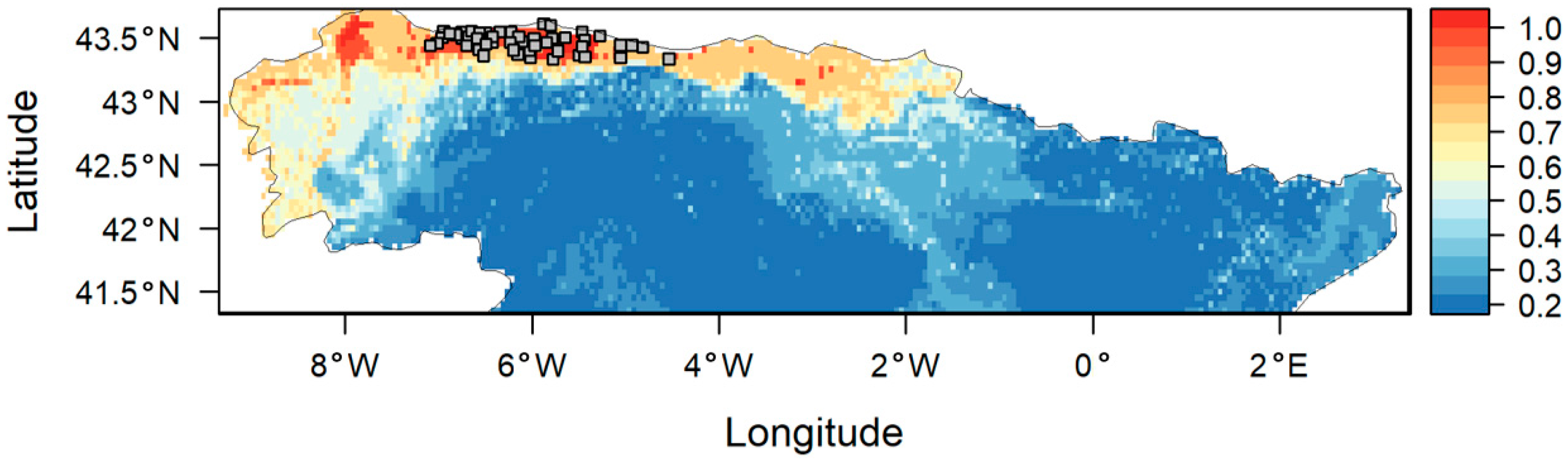
2.1. Study Area
2.2. Data Collection
2.3. Data Preprocessing and Variable Selection
2.4. Spatial Modeling Approach
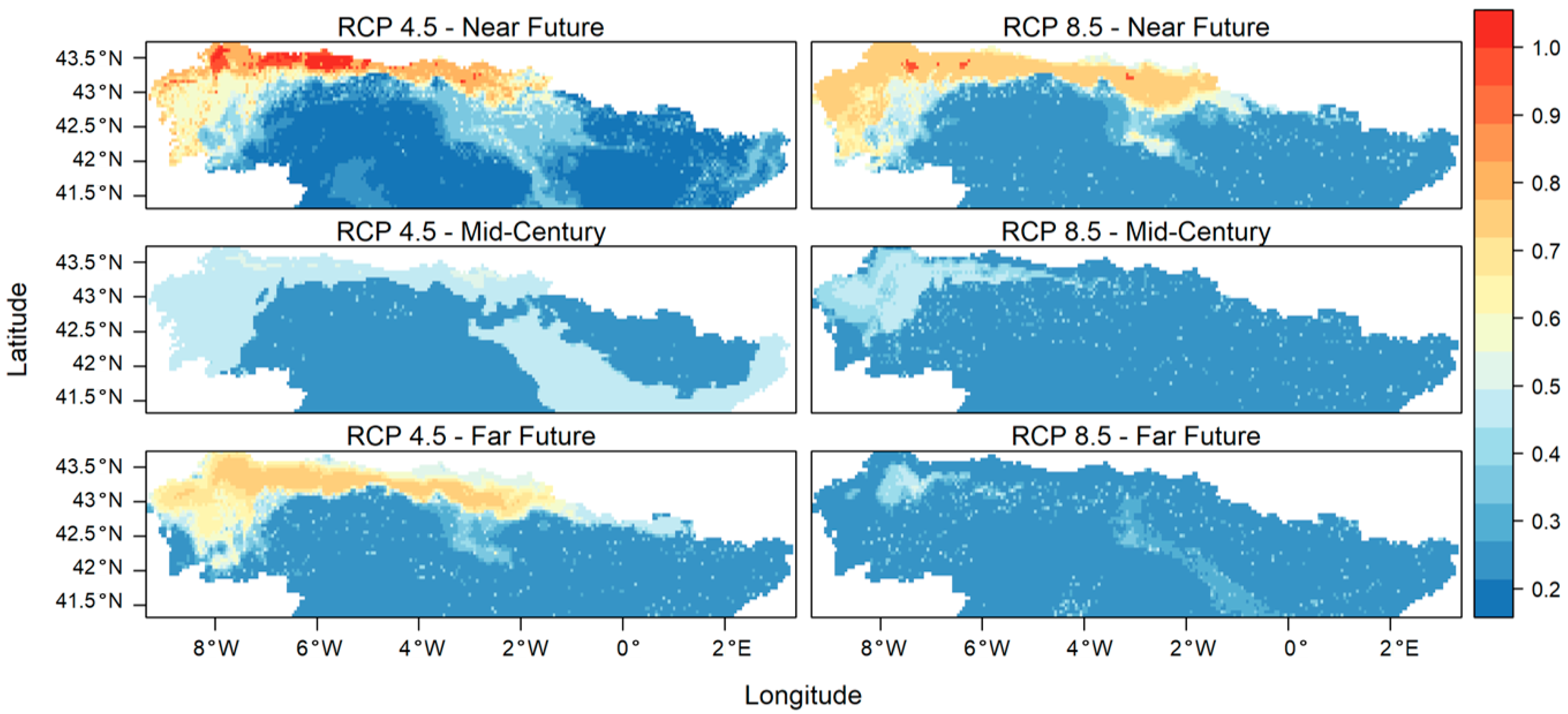
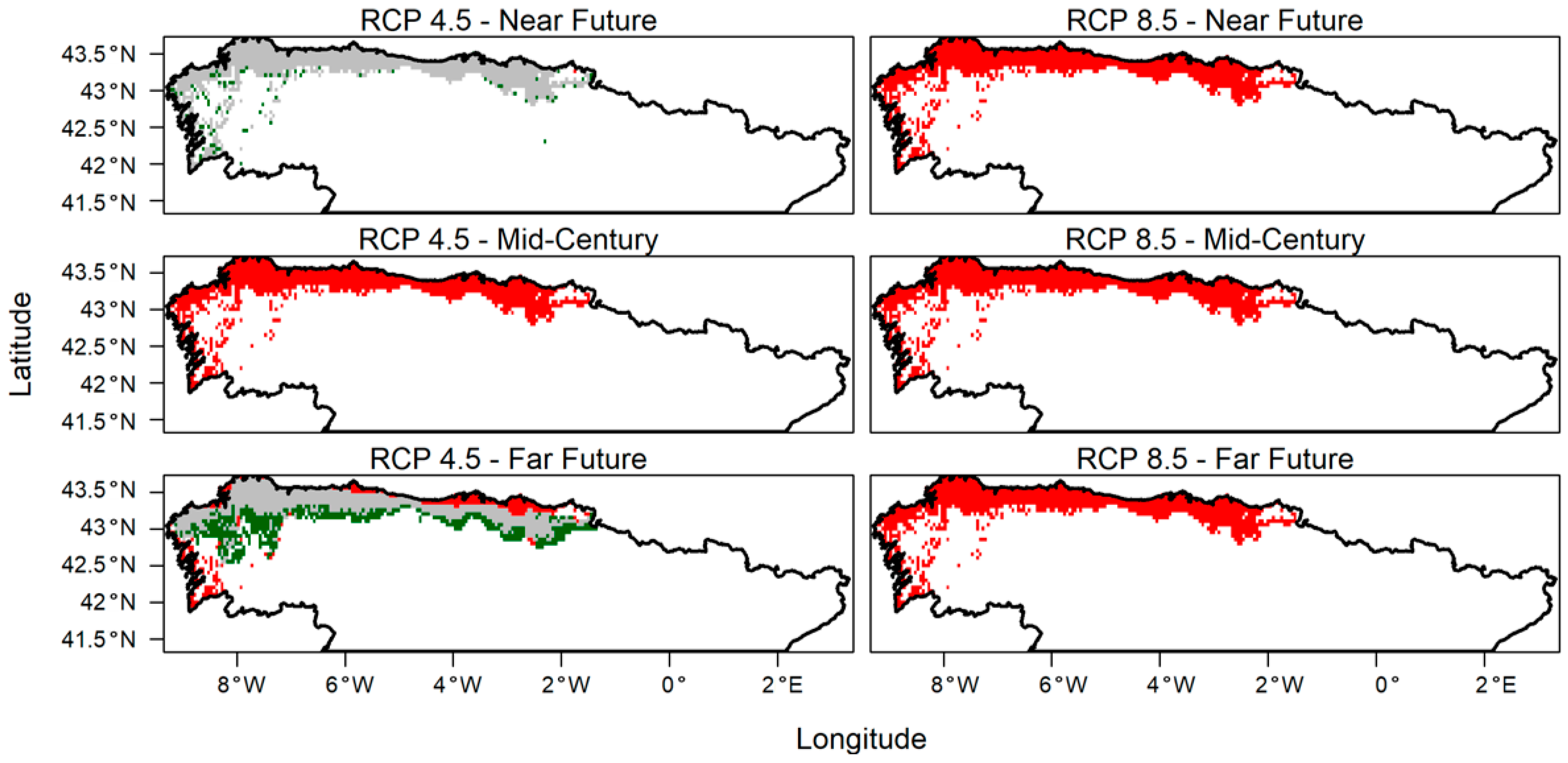
2.5. Application Based on Future Projections
2.6. Ecological Niche Modeling
3. Results
Models and Climatic Stress Variables
4. Discussion
5. Conclusions
Author Contributions
Funding
Institutional Review Board Statement
Data Availability Statement
Conflicts of Interest
Appendix A. SpaMM Model Comparison (Zuur-Based)

| Variables | VIF | |
|---|---|---|
| 1 | prmax24_reference-period | 1.863074 |
| 2 | prspella1_reference-period | 1.660775 |
| 3 | prspellb1_reference-period | 2.780308 |
| 4 | tasdrp99_reference-period | 1.798192 |
| 5 | tasmaxhwdmax_reference-period | 1.534910 |
| 6 | tasmaxnap90_reference-period | 1.002059 |
| 7 | tasminna20_reference-period | 2.069492 |
| 8 | tasminnap90_reference-period | 1.003214 |
| 9 | tasminnb0_reference-period | 2.091630 |
| Variable | Moran’s_I | Expected_I | SD | Z_Score | p_Value | MC_Statistic | MC_p_Value |
|---|---|---|---|---|---|---|---|
| tasminNa20_ reference-period | 0.57522 | −0.0026 | 0.05516 | 10.475 | 5.623 × 10⁻²⁶ | 0.57522 | 0.001 |
| tasminNb0_ reference-period | 0.14038 | −0.0026 | 0.03013 | 4.745 | 1.042 × 10⁻⁶ | 0.14038 | 0.001 |
| prmax24_ reference-period | 0.02025 | −0.0026 | - | - | - | 0.02025 | 0.006 |
| tasmaxhwdmax_reference-period | 0.01167 | −0.0026 | - | - | - | 0.01167 | 0.026 |
| prspella1_ reference-period | 0.00729 | −0.0026 | - | - | - | 0.00729 | 0.061 |
| prspellb1_ reference-period | 0.00716 | −0.0026 | - | - | - | 0.00716 | 0.04 |
| tasdrp99_ reference-period | 0.0068 | −0.0026 | - | - | - | 0.0068 | 0.067 |
| tasmaxNap90_ reference-period | 0.00113 | −0.0026 | - | - | - | 0.00113 | 0.138 |
| tasminNap90_ reference-period | 0.00113 | −0.0026 | - | - | - | 0.00113 | 0.128 |
| Model | Num_Vars | AIC | BIC | logLik | Converged |
|---|---|---|---|---|---|
| tasminNa20_reference-period + tasmaxhwdmax_reference-period + prspellb1_reference-period | 3 | 739.166990956824 | 750.74 | −362.58 | True |
| tasminNa20_reference-period + tasminNb0_reference-period + tasmaxhwdmax_reference-period | 3 | 739.447062239629 | 751.02 | −362.72 | True |
| tasminNa20_reference-period + tasminNb0_reference-period + prmax24_reference-period | 3 | 739.472813210192 | 751.05 | −362.74 | True |
| tasminNa20_reference-period + tasminNb0_reference-period + prspellb1_reference-period | 3 | 739.482841176638 | 751.06 | −362.74 | True |
| tasminNa20_reference-period + prmax24_reference-period + tasmaxhwdmax_reference-period | 3 | 739.536024287047 | 751.11 | −362.77 | True |
| tasminNb0_reference-period + prmax24_reference-period + tasmaxhwdmax_reference-period | 3 | 740.115133947254 | 751.69 | −363.06 | True |
| tasminNb0_reference-period + prmax24_reference-period + prspellb1_reference-period | 3 | 740.124032091255 | 751.7 | −363.06 | True |
| tasminNb0_reference-period + tasmaxhwdmax_reference-period + prspellb1_reference-period | 3 | 740.142324533998 | 751.72 | −363.07 | True |
| tasminNa20_reference-period + prmax24_reference-period + prspellb1_reference-period | 3 | 740.186315918666 | 751.76 | −363.09 | True |
| tasminNa20_reference-period + prmax24_reference-period + tasmaxhwdmax_reference-period + prspellb1_reference-period | 4 | 741.160344975525 | 757.13 | −362.58 | True |
| tasminNa20_reference-period + tasminNb0_reference-period + tasmaxhwdmax_reference-period + prspellb1_reference-period | 4 | 741.163557022221 | 757.13 | −362.58 | True |
| tasminNa20_reference-period + tasminNb0_reference-period + prmax24_reference-period + tasmaxhwdmax_reference-period | 4 | 741.244205182667 | 757.21 | −362.62 | True |
| tasminNa20_reference-period + tasminNb0_reference-period + prmax24_reference-period + prspellb1_reference-period | 4 | 741.358564865126 | 757.33 | −362.68 | True |
| prmax24_reference-period + tasmaxhwdmax_reference-period + prspellb1_reference-period | 3 | 742.002566380944 | 753.58 | −364.0 | True |
| tasminNb0_reference-period + prmax24_reference-period + tasmaxhwdmax_reference-period + prspellb1_reference-period | 4 | 742.044244663033 | 758.01 | −363.02 | True |
| tasminNa20_reference-period + tasminNb0_reference-period + prmax24_reference-period + tasmaxhwdmax_reference-period + prspellb1_reference-period | 5 | 743.148614563252 | 763.51 | −362.57 | True |
References
- Lal, R. Climate change and agriculture. In Climate Change; Elsevier: Amsterdam, The Netherlands, 2021; pp. 661–686. Available online: https://linkinghub.elsevier.com/retrieve/pii/B9780128215753000311 (accessed on 13 May 2025).
- Imtiaz, S.; Shahid, S.; Ishfaq, T.; Ilyas, M.; Nawaz, A.F.; Shamshad, J.; Fahad, S.; Saud, S.; Nawaz, T.; Gu, L.; et al. Impact of Climate Change on Agriculture. In Environment, Climate, Plant and Vegetation Growth; Fahad, S., Saud, S., Nawaz, T., Gu, L., Ahmad, M., Zhou, R., Eds.; Springer Nature: Cham, Switzerland, 2024; pp. 285–305. Available online: https://link.springer.com/10.1007/978-3-031-69417-2_10 (accessed on 12 June 2025).
- Bibi, F.; Rahman, A. An Overview of Climate Change Impacts on Agriculture and Their Mitigation Strategies. Agriculture 2023, 13, 1508. [Google Scholar] [CrossRef]
- Federico, K.; Bonora, A.; Di Giustino, G.; Reho, M.; Lucertini, G. Spatial Analysis of GHG Balances and Climate Change Mitigation in Rural Areas: The Case of Emilia–Romagna Region. Atmosphere 2022, 13, 2060. [Google Scholar] [CrossRef]
- Kumari, A.; Lakshmi, G.A.; Krishna, G.K.; Patni, B.; Prakash, S.; Bhattacharyya, M.; Singh, S.K.; Verma, K.K. Climate Change and Its Impact on Crops: A Comprehensive Investigation for Sustainable Agriculture. Agronomy 2022, 12, 3008. [Google Scholar] [CrossRef]
- Puotinen, M.; Drost, E.; Lowe, R.; Depczynski, M.; Radford, B.; Heyward, A.; Gilmour, J.; Nutt, C.; Muir, P.; Babcock, R.; et al. Towards modelling the future risk of cyclone wave damage to the world’s coral reefs. Glob. Change Biol. 2020, 26, 4302–4315. [Google Scholar] [CrossRef] [PubMed]
- Bouteska, A.; Sharif, T.; Bhuiyan, F.; Abedin, M.Z. Impacts of the changing climate on agricultural productivity and food security: Evidence from Ethiopia. J. Clean. Prod. 2024, 449, 141793. [Google Scholar] [CrossRef]
- Grigorieva, E.; Livenets, A.; Stelmakh, E. Adaptation of Agriculture to Climate Change: A Scoping Review. Climate 2023, 11, 202. [Google Scholar] [CrossRef]
- El Bilali, H.; Kiebre, Z.; Nanema, R.K.; Dan Guimbo, I.; Rokka, V.-M.; Gonnella, M.; Tietiambou, S.R.F.; Dambo, L.; Nanema, J.; Grazioli, F.; et al. Mapping Research on Bambara Groundnut (Vigna subterranea (L.) Verdc.) in Africa: Bibliometric, Geographical, and Topical Perspectives. Agriculture 2024, 14, 1541. [Google Scholar] [CrossRef]
- Ahmed, M.; Sameen, A.; Parveen, H.; Ullah, M.I.; Fahad, S.; Hayat, R. Climate Change Impacts on Legume Crop Production and Adaptation Strategies. In Global Agricultural Production: Resilience to Climate Change; Springer: Cham, Switzerland, 2023. [Google Scholar]
- Climate Change Impacts on Legume Physiology and Ecosystem Dynamics: A Multifaceted Perspective. Sustainability 2024, 16, 6026. [CrossRef]
- Mahto, R.K.; Chandana, B.S.; Singh, R.K.; Talukdar, A.; Swarnalakshmi, K.; Suman, A.; Vaishali; Dey, D.; Kumar, R. Uncovering potentials of an association panel subset for nitrogen fixation and sustainable chickpea productivity. BMC Plant Biol. 2025, 25, 693. [Google Scholar] [CrossRef]
- Jimenez-Lopez, J.C.; Singh, K.B.; Clemente, A.; Nelson, M.N.; Ochatt, S.; Smith, P.M.C. Editorial: Legumes for global food security. Front. Plant Sci. 2020, 11, 926. Available online: https://www.frontiersin.org/articles/10.3389/fpls.2020.00926/full (accessed on 16 July 2025). [CrossRef]
- Stoilova, T.; Simova-Stoilova, L. Bulgarian Cowpea Landraces—Agrobiological and Morphological Characteristics and Seed Biochemical Composition. Agriculture 2024, 14, 2339. [Google Scholar] [CrossRef]
- Al-Tawaha, A.R.M.; Al-Tawaha, A.; Sirajuddin, S.N.; McNeil, D.; Othman, Y.A.; Al-Rawashdeh, I.M.; Amanullah; Imran; Qaisi, A.M.; Jahan, N.; et al. Ecology and adaptation of legumes crops: A review. IOP Conf. Ser. Earth Environ. Sci. 2020, 492, 012085. [Google Scholar] [CrossRef]
- Sippel, S.; Reichstein, M.; Ma, X.; Mahecha, M.D.; Lange, H.; Flach, M.; Frank, D. Drought, heat, and the carbon cycle: A review. Curr. Clim. Change Rep. 2018, 4, 266–286. Available online: https://link.springer.com/article/10.1007/s40641-018-0103-4 (accessed on 16 July 2025). [CrossRef]
- Zhang, L.; Yu, X.; Zhou, T.; Zhang, W.; Hu, S.; Clark, R. Understanding and Attribution of Extreme Heat and Drought Events in 2022: Current Situation and Future Challenges. Adv. Atmos. Sci. 2023, 40, 1941–1951. [Google Scholar] [CrossRef]
- Chapter 11: Weather and Climate Extreme Events in a Changing Climate. Available online: https://www.ipcc.ch/report/ar6/wg1/chapter/chapter-11/ (accessed on 16 July 2025).
- Intergovernmental Panel on Climate Change (IPCC). Climate Change 2022—Impacts, Adaptation and Vulnerability: Working Group II Contribution to the Sixth Assessment Report of the Intergovernmental Panel on Climate Change, 1st ed.; Cambridge University Press: Cambridge, UK, 2023; Available online: https://www.cambridge.org/core/product/identifier/9781009325844/type/book (accessed on 15 May 2025).
- Pendergrass, A.G.; Meehl, G.A.; Pulwarty, R.; Hobbins, M.; Hoell, A.; AghaKouchak, A.; Bonfils, C.J.W.; Gallant, A.J.E.; Hoerling, M.; Hoffmann, D.; et al. Flash Droughts Present a New Challenge for Subseasonal-to-Seasonal Prediction. Nat. Clim. Change 2020, 10, 191–199. [Google Scholar] [CrossRef]
- European Commission. Reglamentos sobre Indicaciones Geográficas. 2023. Available online: https://agriculture.ec.europa.eu/farming/geographical-indications-and-quality-schemes/regulations-gis_es (accessed on 15 May 2025).
- Rackl, J.; Menapace, L. Coordination in Agri-Food Supply Chains: The Role of Geographical Indication Certification. Int. J. Prod. Econ. 2025, 280, 109494. [Google Scholar] [CrossRef]
- Rahman, M.M.; Alam, M.S.; Islam, M.M.; Kamal, M.Z.U.; Rahman, G.K.M.M.; Haque, M.M.; Miah, M.G.; Biswas, J.C. Potential of Legume-Based Cropping Systems for Climate Change Adaptation and Mitigation. In Advances in Legumes for Sustainable Intensification; Elsevier: Amsterdam, The Netherlands, 2022; pp. 381–402. Available online: https://linkinghub.elsevier.com/retrieve/pii/B9780323857970000306 (accessed on 13 May 2025).
- Zou, Y.; Liu, Z.; Chen, Y.; Wang, Y.; Feng, S. Crop Rotation and Diversification in China: Enhancing Sustainable Agriculture and Resilience. Agriculture 2024, 14, 1465. [Google Scholar] [CrossRef]
- Romaneckas, K.; Švereikaitė, A.; Kimbirauskienė, R.; Sinkevičienė, A.; Adamavičienė, A.; Jasinskas, A. The Impact of Maize Legume Intercropping on Energy Indices and GHG Emissions as a Result of Climate Change. Agriculture 2024, 14, 1303. [Google Scholar] [CrossRef]
- Selje, T.; Schmid, L.A.; Heinz, B. Community-Based Adaptation to Climate Change: Core Issues and Implications for Practical Implementations. Climate 2024, 12, 155. [Google Scholar] [CrossRef]
- Kapruwan, R.; Saksham, A.K.; Ford, J.D.; Petzold, J.; McDowell, G.; Rufat, S.; Schneiderbauer, S.; Tiwari, S.; Pandey, R. Climate change adaptation in global mountain regions requires a multi-sectoral approach. Commun. Earth Environ. 2025, 6, 454. [Google Scholar] [CrossRef]
- Thomas, A.; Theokritoff, E.; Lesnikowski, A.; Reckien, D.; Jagannathan, K.; Cremades, R.; Campbell, D.; Joe, E.T.; Sitati, A.; Singh, C.; et al. Global evidence of constraints and limits to human adaptation. Reg. Environ. Change 2021, 21, 85. [Google Scholar] [CrossRef]
- Berbés-Blázquez, M.; Mitchell, C.L.; Burch, S.L.; Wandel, J. Understanding climate change and resilience: Assessing strengths and opportunities for adaptation in the Global South. Clim. Change 2017, 141, 227–241. [Google Scholar] [CrossRef]
- Montsant, A.; Baena, O.; Bernárdez, L.; Puig, J. Modelling the impacts of climate change on potential cultivation area and water deficit in five Mediterranean crops. Span. J. Agric. Res. 2021, 19, e0301. [Google Scholar] [CrossRef]
- Dubey, P.K.; Singh, G.S.; Abhilash, P.C. Adaptive Agricultural Practices: Building Resilience in a Changing Climate; SpringerBriefs in Environmental Science; Springer International Publishing: Cham, Switzerland, 2020; Available online: http://link.springer.com/10.1007/978-3-030-15519-3 (accessed on 12 June 2025).
- BOE-A-2019-5481; Ley 2/2019, de 1 de Marzo, de Calidad Alimentaria, Calidad Diferenciada y Venta Directa de Productos Alimentarios. Agencia Estatal Boletín Oficial del Estado: Madrid, Spain, 2019. Available online: https://www.boe.es/buscar/act.php?id=BOE-A-2019-5481 (accessed on 15 May 2025).
- Farooq, A.; Farooq, N.; Akbar, H.; Hassan, Z.U.; Gheewala, S.H. A Critical Review of Climate Change Impact at a Global Scale on Cereal Crop Production. Agronomy 2023, 13, 162. [Google Scholar] [CrossRef]
- Feng, X.; Tian, H.; Cong, J.; Zhao, C. A method review of the climate change impact on crop yield. Front. For. Glob. Change 2023, 6, 1198186. [Google Scholar] [CrossRef]
- Li, J.; Ma, W.; Zhu, H. A systematic literature review of factors influencing the adoption of climate-smart agricultural practices. Mitig. Adapt. Strateg. Glob. Change 2024, 29, 2. [Google Scholar] [CrossRef]
- Hatfield, J.L.; Prueger, J.H. Temperature extremes: Effect on plant growth and development. Weather Clim. Extrem. 2015, 10, 4–10. [Google Scholar] [CrossRef]
- Schlenker, W.; Roberts, M.J. Nonlinear temperature effects indicate severe damages to U.S. crop yields under climate change. Proc. Natl. Acad. Sci. USA 2009, 106, 15594–15598. [Google Scholar] [CrossRef]
- Abobatta, W.F.; ElHashash, F.; Hegab, H. Challenges and Opportunities for the Global Cultivation and Adaption of Legumes. J. Appl. Biotechnol. Bioeng. 2021, 8, 160–172. [Google Scholar] [CrossRef]
- Singer, S.D.; Chatterton, S.; Soolanayakanahally, R.Y.; Subedi, U.; Chen, G.; Acharya, S.N. Potential Effects of a High CO2 Future on Leguminous Species. Plant Environ. Interact. 2020, 1, 67–94. [Google Scholar] [CrossRef]
- Sollenberger, L.E.; Kohmann, M.M. Forage Legume Responses to Climate Change Factors. Crop. Sci. 2024, 64, 2419–2432. [Google Scholar] [CrossRef]
- Du, S.; Luo, X.; Tang, L.; Yan, A. The effects of quality certification on agricultural low-carbon production behavior: Evidence from Chinese rice farmers. Int. J. Agric. Sustain. 2023, 21, 2227797. [Google Scholar] [CrossRef]
- Alae-Carew, C.; Nicoleau, S.; Bird, F.A.; Hawkins, P.; Tuomisto, H.L.; Haines, A.; Dangour, A.D. The impact of environmental changes on the yield and nutritional quality of fruits, nuts and seeds: A systematic review. Environ. Res. Lett. 2020, 15, 023002. [Google Scholar] [CrossRef]
- Shankar, K.S.; Vanaja, M.; Shankar, M.; Siddiqua, A.; Sharma, K.L.; Girijaveni, V.; Singh, V.K. Change in mineral composition and cooking quality in legumes grown on semi-arid alfisols due to elevated CO2 and temperature. Front. Nutr. 2025, 11, 1444962. [Google Scholar] [CrossRef]
- Lulovicova, A.; Bouissou, S. Life cycle assessment as a prospective tool for sustainable agriculture and food planning at a local level. Geogr. Sustain. 2024, 5, 251–264. [Google Scholar] [CrossRef]
- Vandecandelaere, E.; Teyssier, C.; Marescotti, A. Strengthening Sustainable Food Systems Through Geographical Indications: An Analysis of Climate Resilience in GI Value Chains; FAO & EBRD: Rome, Italy, 2022; Available online: https://openknowledge.fao.org/handle/20.500.14283/cc2742en (accessed on 4 June 2025).
- Mietz, L.K.; Civit, B.M.; Arena, A.P. Life cycle assessment to evaluate the sustainability of urban agriculture: Opportunities and challenges. Agroecol. Sustain. Food Syst. 2024, 48, 983–1007. [Google Scholar] [CrossRef]
- Canaj, K.; Parente, A.; D’Imperio, M.; Boari, F.; Buono, V.; Toriello, M.; Mehmeti, A.; Montesano, F.F. Can Precise Irrigation Support the Sustainability of Protected Cultivation? A Life-Cycle Assessment and Life-Cycle Cost Analysis. Water 2021, 14, 6. [Google Scholar] [CrossRef]
- High Level Panel of Experts on Food Security and Nutrition (HLPE). Food Security and Nutrition: Building a Global Narrative Towards 2030; Committee on World Food Security (CFS): Rome, Italy, 2020; Available online: https://www.fao.org/3/ca9731en/ca9731en.pdf (accessed on 4 June 2025).
- Horoszkiewicz, J.; Jajor, E.; Danielewicz, J.; Korbas, M.; Schimmelpfennig, L.; Mikos-Szymańska, M.; Klimczyk, M.; Bocianowski, J. The Assessment of an Effect of Natural Origin Products on the Initial Growth and Development of Maize under Drought Stress and the Occurrence of Selected Pathogens. Agriculture 2023, 13, 815. [Google Scholar] [CrossRef]
- Hammond, R.A.; Dubé, L. A systems science perspective and transdisciplinary models for food and nutrition security. Proc. Natl. Acad. Sci. USA 2012, 109, 12356–12363. [Google Scholar] [CrossRef]
- Ericksen, P.J. Conceptualizing food systems for global environmental change research. Glob. Environ. Change 2008, 18, 234–245. [Google Scholar] [CrossRef]
- Kracht, C.L.; Swyden, K.J.; Weedn, A.E.; Salvatore, A.L.; Terry, R.A.; Sisson, S.B. A Structural Equation Modelling Approach to Understanding Influences of Maternal and Family Characteristics on Feeding Practices in Young Children. Curr. Dev. Nutr. 2018, 2, nzy061. [Google Scholar] [CrossRef] [PubMed]
- United Nations. Transforming Our World: The 2030 Agenda for Sustainable Development. Available online: https://sdgs.un.org/2030agenda (accessed on 3 June 2025).
- Sustainable Food Systems Conference, June 2016. Available online: https://en-lifesci.tau.ac.il/food/news/foodsystemsconference2016 (accessed on 14 May 2025).
- Pilling, D.; Bélanger, J. The State of the World’s Biodiversity for Food and Agriculture; Food and Agriculture Organization: Rome, Italy, 2019. [Google Scholar]
- Willett, W.; Rockström, J.; Loken, B.; Springmann, M.; Lang, T.; Vermeulen, S.; Garnett, T.; Tilman, D.; DeClerck, F.; Wood, A.; et al. Food in the Anthropocene: The EAT–Lancet Commission on healthy diets from sustainable food systems. Lancet 2019, 393, 447–492. [Google Scholar] [CrossRef]
- European Commission. A Farm to Fork Strategy for a Fair, Healthy and Environmentally-Friendly Food System; European Commission: Brussels, Belgium, 2020; Available online: https://food.ec.europa.eu/system/files/2020-05/f2f_action-plan_2020_strategy-info_en.pdf (accessed on 14 May 2025).
- Food and Agriculture Organization of the United Nations (FAO). Geographical Indications for Sustainable Food Systems; FAO: Rome, Italy, 2021; Available online: https://openknowledge.fao.org/handle/20.500.14283/cb3702en (accessed on 4 June 2025).
- Magrini, M.-B.; Anton, M.; Chardigny, J.-M.; Duc, G.; Duru, M.; Jeuffroy, M.-H.; Meynard, J.-M.; Micard, V.; Walrand, S. Pulses for Sustainability: Breaking agriculture and food sectors out of lock-in. Front. Sustain. Food Syst. 2018, 2, 64. [Google Scholar] [CrossRef]
- Costa, M.P.; Reckling, M.; Chadwick, D.; Rees, R.M.; Saget, S.; Williams, M.; Styles, D. Legume-Modified Rotations Deliver Nutrition with Lower Environmental Impact. Front. Sustain. Food Syst. 2021, 5, 656005. [Google Scholar] [CrossRef]
- Pelzer, E.; Bourlet, C.; Carlsson, G.; Lopez-Bellido, R.J.; Jensen, E.S.; Jeuffroy, M.-H. Design, assessment and feasibility of legume-based cropping systems in three European regions. Crop Pasture Sci. 2017, 68, 902. [Google Scholar] [CrossRef]
- Wang, X.; Zhao, C.; Müller, C.; Wang, C.; Ciais, P.; Janssens, I.A.; Peñuelas, J.; Asseng, S.; Li, T.; Elliott, J.; et al. Emergent constraint on crop yield response to warmer temperature from field experiments. Nat. Sustain. 2020, 3, 908–916. [Google Scholar] [CrossRef]
- Austin, K.G.; Beach, R.H.; Lapidus, D.; Salem, M.E.; Taylor, N.J.; Knudsen, M.; Ujeneza, N. Impacts of Climate Change on the Potential Productivity of Eleven Staple Crops in Rwanda. Sustainability 2020, 12, 4116. [Google Scholar] [CrossRef]
- Xu, Q.; Liang, H.; Wei, Z.; Zhang, Y.; Lu, X.; Li, F.; Wei, N.; Zhang, S.; Yuan, H.; Liu, S.; et al. Assessing Climate Change Impacts on Crop Yields and Exploring Adaptation Strategies in Northeast China. Earth’s Future 2024, 12, e2023EF004063. [Google Scholar] [CrossRef]
- Hu, Y.; Ma, P.; Yang, Z.; Liu, S.; Li, Y.; Li, L.; Wang, T.; Siddique, K.H.M. The Responses of Crop Yield and Greenhouse Gas Emissions to Straw Returning from Staple Crops: A Meta-Analysis. Agriculture 2025, 15, 408. [Google Scholar] [CrossRef]
- Schmidt, M.; Felsche, E. The effect of climate change on crop yield anomaly in Europe. Clim. Resil. Sustain. 2024, 3, e61. [Google Scholar] [CrossRef]
- Scialabba, N.E.-H.; Müller-Lindenlauf, M. Organic agriculture and climate change. Renew. Agric. Food Syst. 2010, 25, 158–169. [Google Scholar] [CrossRef]
- Marescotti, A.; Quiñones-Ruiz, X.F.; Edelmann, H.; Belletti, G.; Broscha, K.; Altenbuchner, C.; Penker, M.; Scaramuzzi, S. Are Protected Geographical Indications Evolving Due to Environmentally Related Justifications? An Analysis of Amendments in the Fruit and Vegetable Sector in the European Union. Sustainability 2020, 12, 3571. [Google Scholar] [CrossRef]
- Gaydon, D.S.; Radanielson, A.M.; Chaki, A.K.; Sarker, M.M.R.; Rahman, M.A.; Rashid, M.H.; Roth, C.H.; Poulton, P.L.; Mainuddin, M.; Nelson, R.; et al. Options for increasing Boro rice production in the saline coastal zone of Bangladesh. Field Crops Res. 2021, 264, 108089. [Google Scholar] [CrossRef]
- Alvar-Beltrán, J.; Dibari, C.; Ferrise, R.; Bartoloni, N.; Marta, A.D. Modelling climate change impacts on crop production in food insecure regions: The case of Niger. Eur. J. Agron. 2023, 142, 126667. [Google Scholar] [CrossRef]
- Kagnew, B.; Assefa, A.; Degu, A. Modeling the Impact of Climate Change on Sustainable Production of Two Legumes Important Economically and for Food Security: Mungbeans and Cowpeas in Ethiopia. Sustainability 2022, 15, 600. [Google Scholar] [CrossRef]
- Thaler, S.; Brocca, L.; Ciabatta, L.; Eitzinger, J.; Hahn, S.; Wagner, W. Effects of Different Spatial Precipitation Input Data on Crop Model Outputs under a Central European Climate. Atmosphere 2018, 9, 290. [Google Scholar] [CrossRef]
- Kim, Y.; Evans, J.P.; Sharma, A.; Rocheta, E. Spatial, Temporal, and Multivariate Bias in Regional Climate Model Simulations. Geophys. Res. Lett. 2021, 48, e2020GL092058. [Google Scholar] [CrossRef]
- Peng, Y.; Xin, J.; Peng, N.; Li, Y.; Huang, J.; Zhang, R.; Zhang, Y.; Wang, X.; Fang, J.; Zhang, Y. Global patterns and drivers of spatial autocorrelation in plant communities in protected areas. Divers. Distrib. 2024, 30, 119–133. [Google Scholar] [CrossRef]
- Holzkämper, A. Adapting Agricultural Production Systems to Climate Change—What’s the Use of Models? Agriculture 2017, 7, 86. [Google Scholar] [CrossRef]
- Kherif, O.; Haddad, B.; Bouras, F.-Z.; Seghouani, M.; Zemmouri, B.; Gamouh, R.; Hamzaoui, N.; Larbi, A.; Rebouh, N.-Y.; Latati, M. Simultaneous Assessment of Water and Nitrogen Use Efficiency in Rain-Fed Chickpea-Durum Wheat Intercropping Systems. Agriculture 2023, 13, 947. [Google Scholar] [CrossRef]
- Timlin, D.; Paff, K.; Han, E. The role of crop simulation modeling in assessing potential climate change impacts. Agrosystems Geosci. Environ. 2024, 7, e20453. [Google Scholar] [CrossRef]
- Hannah, L.; Donatti, C.I.; Harvey, C.A.; Alfaro, E.; Rodriguez, D.A.; Bouroncle, C.; Castellanos, E.; Diaz, F.; Fung, E.; Hidalgo, H.G.; et al. Regional modeling of climate change impacts on smallholder agriculture and ecosystems in Central America. Clim. Change 2017, 141, 29–45. [Google Scholar] [CrossRef]
- Hijmans, R.J. Cross-validation of species distribution models: Removing spatial sorting bias and calibration with a null model. Ecology 2012, 93, 679–688. [Google Scholar] [CrossRef]
- Bivand, R.S.; Pebesma, E.; Gómez-Rubio, V. Applied Spatial Data Analysis with R; Springer: New York, NY, USA, 2013; Available online: https://link.springer.com/10.1007/978-1-4614-7618-4 (accessed on 3 June 2025).
- Lake, L.; Godoy-Kutchartt, D.E.; Calderini, D.F.; Verrell, A.; Sadras, V.O. Yield determination and the critical period of faba bean (Vicia faba L.). Field Crops Res. 2019, 241, 107575. [Google Scholar] [CrossRef]
- Panda, S.S.; Terrill, T.H.; Mahapatra, A.K.; Morgan, E.R.; Siddique, A.; Pech-Cervantes, A.A.; van Wyk, J.A. Optimizing Sericea Lespedeza Fodder Production in the Southeastern US: A Climate-Informed Geospatial Engineering Approach. Agriculture 2023, 13, 1661. [Google Scholar] [CrossRef]
- Pirasteh, S.; Fang, Y.; Mafi-Gholami, D.; Abulibdeh, A.; Nouri-Kamari, A.; Khonsari, N. Enhancing vulnerability assessment through spatially explicit modeling of mountain social-ecological systems exposed to multiple environmental hazards. Sci. Total Environ. 2024, 930, 172744. [Google Scholar] [CrossRef] [PubMed]
- Balko, C.; Torres, A.M.; Gutierrez, N. Variability in drought stress response in a panel of 100 faba bean genotypes. Front. Plant Sci. 2023, 14, 1236147. [Google Scholar] [CrossRef]
- Dou, Y.; Tong, X.; Horion, S.; Feng, L.; Fensholt, R.; Shao, Q.; Brandt, M. The success of ecological engineering projects on vegetation restoration in China strongly depends on climatic conditions. Sci. Total Environ. 2024, 915, 170041. [Google Scholar] [CrossRef] [PubMed]
- Köppen, W.; Geiger, R. The geographical system of climates. In Handbook of Climatology (Handbuch der Klimatologie); Gebrüder Borntraeger: Berlin, Germany, 1936. [Google Scholar]
- Pérez, R.; Fernández, C.; Laca, A.; Laca, A. Evaluation of Environmental Impacts in Legume Crops: A Case Study of PGI White Bean Production in Southern Europe. Sustainability 2024, 16, 8024. [Google Scholar] [CrossRef]
- Dirección General de Política Alimentaria (España). Resolución de 15 de Enero de 1990, de la Dirección General de Política Alimentaria, por la que se Reconoce la Denominación Específica Faba Asturiana y su Reglamento. Available online: https://www.boe.es/boe/dias/1990/02/10/pdfs/A04150-04150.pdf (accessed on 24 July 2025).
- Zheng, C.; Zhang, J.; Chen, J.; Chen, C.; Tian, Y.; Deng, A.; Cao, W.; Zhang, W. Nighttime warming increases winter-sown wheat yield across major Chinese cropping regions. Field Crops Res. 2017, 214, 202–210. [Google Scholar] [CrossRef]
- Shelef, O.; Weisberg, P.J.; Provenza, F.D. The Value of Native Plants and Local Production in an Era of Global Agriculture. Front. Plant Sci. 2017, 8, 2069. [Google Scholar] [CrossRef]
- BOE-A-1990-16900; Orden de 6 de Julio de 1990 por la que se Ratifica el Reglamento de la denominación Específica Faba Asturiana y de su Consejo Regulador. Agencia Estatal Boletín Oficial del Estado: Madrid, Spain, 1990. Available online: https://www.boe.es/diario_boe/txt.php?id=BOE-A-1990-16900 (accessed on 16 July 2025).
- Law No. 6/2015 of May 12, 2015, on Protected Designations of Origin and Geographical Indications of Supra-Autonomic Territory, Spain, WIPO Lex. Available online: https://www.wipo.int/wipolex/en/legislation/details/17241 (accessed on 15 May 2025).
- Thompson, W.J.; Blaser-Hart, W.J.; Joerin, J.; Krütli, P.; Dawoe, E.; Kopainsky, B.; Chavez, E.; Garrett, R.D.; Six, J. Can sustainability certification enhance the climate resilience of smallholder farmers? The case of Ghanaian cocoa. J. Land Use Sci. 2022, 17, 407–428. [Google Scholar] [CrossRef]
- Kang, S.; Frick, F.; Ait Sidhoum, A.; Sauer, J.; Zheng, S. Does food quality certification improve eco-efficiency? Empirical evidence from Chinese vegetable production. Food Policy 2023, 121, 102564. [Google Scholar] [CrossRef]
- IPCC. AR5 Synthesis Report: Climate Change 2014. Available online: https://www.ipcc.ch/report/ar5/syr/ (accessed on 16 July 2025).
- IPCC. Chapter 4—AR6 Climate Change 2021: The Physical Science Basis. Available online: https://www.ipcc.ch/report/ar6/wg1/chapter/chapter-4/ (accessed on 16 July 2025).
- Ylänne, H.; Madsen, R.L.; Castaño, C.; Metcalfe, D.B.; Clemmensen, K.E. Reindeer control over subarctic treeline alters soil fungal communities with potential consequences for soil carbon storage. Glob. Change Biol. 2021, 27, 4254–4268. [Google Scholar] [CrossRef] [PubMed]
- Law, E.P.; Wayman, S.; Pelzer, C.J.; Culman, S.W.; Gómez, M.I.; DiTommaso, A.; Ryan, M.R. Multi-Criteria Assessment of the Economic and Environmental Sustainability Characteristics of Intermediate Wheatgrass Grown as a Dual-Purpose Grain and Forage Crop. Sustainability 2022, 14, 3548. [Google Scholar] [CrossRef]
- Sosinski, S.; Castillo, M.S.; Kulesza, S.; Leon, R. Poultry litter and nitrogen fertilizer effects on productivity and nutritive value of crabgrass. Crop Sci. 2022, 62, 2537–2547. [Google Scholar] [CrossRef]
- Esri. Selecting and Extracting Data—ArcMap|Documentation. Available online: https://desktop.arcgis.com/en/arcmap/latest/analyze/commonly-used-tools/extracting-data.htm (accessed on 16 July 2025).
- Plataforma sobre Adaptación al Cambio Climático en España. What is AdapteCCa? Available online: https://adaptecca.es/en/what-adaptecca (accessed on 16 July 2025).
- Naimi, B. Usdm: Uncertainty Analysis for Species Distribution Models 2012. Available online: https://CRAN.R-project.org/package=usdm (accessed on 27 May 2025).
- R Core Team. R: The R Project for Statistical Computing. Available online: https://www.r-project.org/ (accessed on 15 June 2025).
- Moran, P.A.P. Notes on continuous stochastic phenomena. Biometrika 1950, 37, 17–23. [Google Scholar] [CrossRef]
- Pebesma, E.J.; Bivand, R.S. Classes and Methods for Spatial Data in R. R News 2005, 5, 9–13. [Google Scholar]
- Cappello, C.; De Iaco, S.; Palma, M. Computational advances for spatio-temporal multivariate environmental models. Comput. Stat. 2022, 37, 651–670. [Google Scholar] [CrossRef]
- Rousset, F.; Ferdy, J. Testing environmental and genetic effects in the presence of spatial autocorrelation. Ecography 2014, 37, 781–790. [Google Scholar] [CrossRef]
- Zuur, A.F.; Ieno, E.N.; Walker, N.; Saveliev, A.A.; Smith, G.M. Mixed Effects Models and Extensions in Ecology with R; Statistics for Biology and Health; Springer: New York, NY, USA, 2009; Available online: http://link.springer.com/10.1007/978-0-387-87458-6 (accessed on 27 May 2025).
- Akaike, H. A new look at the statistical model identification. IEEE Trans. Autom. Control 1974, 19, 716–723. [Google Scholar] [CrossRef]
- Merow, C.; Smith, M.J.; Silander, J.A. A practical guide to MaxEnt for modeling species’ distributions: What it does, and why inputs and settings matter. Ecography 2013, 36, 1058–1069. [Google Scholar] [CrossRef]
- Mestre-Tomás, J. GeoThinneR: An R Package for Efficient Spatial Thinning of Species Occurrences and Point Data. arXiv 2025, arXiv:2505.07867. Available online: https://arxiv.org/abs/2505.07867 (accessed on 16 July 2025).
- Sillero, N.; Arenas-Castro, S.; Enriquez-Urzelai, U.; Vale, C.G.; Sousa-Guedes, D.; Martínez-Freiría, F.; Real, R.; Barbosa, A.M. Want to model a species niche? A step-by-step guideline on correlative ecological niche modelling. Ecol. Model. 2021, 456, 109671. [Google Scholar] [CrossRef]
- Fourcade, Y.; Engler, J.O.; Rödder, D.; Secondi, J. Mapping species distributions with MAXENT using a geographically biased sample of presence data: A performance assessment of methods for correcting sampling bias. PLoS ONE 2014, 9, e97122. [Google Scholar] [CrossRef]
- Aiello-Lammens, M.E.; Boria, R.A.; Radosavljevic, A.; Vilela, B.; Anderson, R.P. spThin: An R package for spatial thinning of species occurrence records for use in ecological niche models. Ecography 2015, 38, 541–545. [Google Scholar] [CrossRef]
- Naimi, B.; Araújo, M.B. sdm: A reproducible and extensible R platform for species distribution modelling. Ecography 2016, 39, 368–375. [Google Scholar] [CrossRef]
- Busby, J.R. Bioclim, a bioclimatic analysis and prediction system. In Nature Conservation: Cost Effective Biological Surveys and Data Analysis; Margules, C.R., Austin, M.P., Eds.; CSIRO: Canberra, Australia, 1991; pp. 64–68. [Google Scholar]
- McCullagh, P.; Nelder, J.A. Generalized Linear Models, 2nd ed.; Routledge: London, UK, 2019; Available online: https://www.taylorfrancis.com/books/9781351445856 (accessed on 11 June 2025).
- Friedman, J.H. Greedy function approximation: A gradient boosting machine. Ann. Stat. 2001, 29, 1189–1232. Available online: https://projecteuclid.org/journals/annals-of-statistics/volume-29/issue-5/Greedy-function-approximation-A-gradient-boosting-machine/10.1214/aos/1013203451.full (accessed on 11 June 2025). [CrossRef]
- Breiman, L. Random Forests. Mach. Learn. 2001, 45, 5–32. [Google Scholar] [CrossRef]
- Phillips, S.J.; Anderson, R.P.; Schapire, R.E. Maximum entropy modeling of species geographic distributions. Ecol. Model. 2006, 190, 231–259. [Google Scholar] [CrossRef]
- Estopinan, J.; Servajean, M.; Bonnet, P.; Munoz, F.; Joly, A. Deep species distribution modeling from Sentinel-2 image time-series: A global scale analysis on the orchid family. Front. Plant Sci. 2022, 13, 839327. [Google Scholar] [CrossRef]
- Ramirez-Villegas, J.; Molero Milan, A.; Alexandrov, N.; Asseng, S.; Challinor, A.J.; Crossa, J.; van Eeuwijk, F.; Ghanem, M.E.; Grenier, C.; Heinemann, A.B.; et al. CGIAR modeling approaches for resource-constrained scenarios: I. Accelerating crop breeding for a changing climate. Crop Sci. 2020, 60, 547–567. [Google Scholar] [CrossRef]
- Wheeler, T.R.; Craufurd, P.Q.; Ellis, R.H.; Porter, J.R.; Vara Prasad, P.V. Temperature variability and the yield of annual crops. Agric. Ecosyst. Environ. 2000, 82, 159–167. [Google Scholar] [CrossRef]
- Prasad, P.V.V.; Boote, K.J.; Allen, L.H.; Thomas, J.M.G. Effects of elevated temperature and carbon dioxide on seed-set and yield of kidney bean (Phaseolus vulgaris L.). Glob. Change Biol. 2002, 8, 710–721. [Google Scholar] [CrossRef]
- Sita, K.; Sehgal, A.; HanumanthaRao, B.; Nair, R.M.; Vara Prasad, P.V.; Kumar, S.; Gaur, P.M.; Farooq, M.; Siddique, K.H.M.; Varshney, R.K.; et al. Food legumes and rising temperatures: Effects, adaptive functional mechanisms specific to reproductive growth stage and strategies to improve heat tolerance. Front. Plant Sci. 2017, 8, 1658. [Google Scholar] [CrossRef] [PubMed]
- Manning, B.K.; Trethowan, R.; Adhikari, K.N. Impact of temperature on podding in faba bean (Vicia faba). Agronomy 2024, 14, 2309. [Google Scholar] [CrossRef]
- Liu, Y.; Li, J.; Zhu, Y.; Jones, A.; Rose, R.J.; Song, Y. Heat stress in legume seed setting: Effects, causes, and future prospects. Front. Plant Sci. 2019, 10, 938. [Google Scholar] [CrossRef] [PubMed]
- El Haddad, N.; Choukri, H.; Ghanem, M.E.; Smouni, A.; Mentag, R.; Rajendran, K.; Hejjaoui, K.; Maalouf, F.; Kumar, S. High-temperature and drought stress effects on growth, yield and nutritional quality with transpiration response to vapor pressure deficit in lentil. Plants 2021, 11, 95. [Google Scholar] [CrossRef]
- Farooq, M.; Nadeem, F.; Gogoi, N.; Ullah, A.; Alghamdi, S.S.; Nayyar, H.; Siddique, K.H.M. Heat stress in grain legumes during reproductive and grain-filling phases. Crop Pasture Sci. 2017, 68, 985. [Google Scholar] [CrossRef]
- Lobell, D.B.; Gourdji, S.M. The influence of climate change on global crop productivity. Plant Physiol. 2012, 160, 1686–1697. [Google Scholar] [CrossRef]
- Lesk, C.; Rowhani, P.; Ramankutty, N. Influence of extreme weather disasters on global crop production. Nature 2016, 529, 84–87. [Google Scholar] [CrossRef]
- Fraga, H.; Malheiro, A.C.; Moutinho-Pereira, J.; Santos, J.A. Future scenarios for viticultural zoning in Europe: Ensemble projections and uncertainties. Int. J. Biometeorol. 2013, 57, 909–925. [Google Scholar] [CrossRef]
- Vadez, V.; Berger, J.D.; Warkentin, T.; Asseng, S.; Ratnakumar, P.; Rao, K.P.C.; Gaur, P.M.; Munier-Jolain, N.; Larmure, A.; Voisin, A.-S.; et al. Adaptation of grain legumes to climate change: A review. Agron. Sustain. Dev. 2012, 32, 31–44. [Google Scholar] [CrossRef]
- Urban, M.C.; Bocedi, G.; Hendry, A.P.; Mihoub, J.-B.; Pe’er, G.; Singer, A.; Bridle, J.R.; Crozier, L.G.; De Meester, L.; Godsoe, W.; et al. Improving the forecast for biodiversity under climate change. Science 2016, 353, aad8466. [Google Scholar] [CrossRef] [PubMed]
- Schauberger, B.; Archontoulis, S.; Arneth, A.; Balkovic, J.; Ciais, P.; Deryng, D.; Elliott, J.; Folberth, C.; Khabarov, N.; Müller, C.; et al. Consistent negative response of US crops to high temperatures in observations and crop models. Nat. Commun. 2017, 8, 13931. [Google Scholar] [CrossRef]
- Hawkins, E.; Sutton, R. The potential to narrow uncertainty in regional climate predictions. Bull. Am. Meteorol. Soc. 2009, 90, 1095–1108. [Google Scholar] [CrossRef]
- Riahi, K.; Rao, S.; Krey, V.; Cho, C.; Chirkov, V.; Fischer, G.; Kindermann, G.; Nakicenovic, N.; Rafaj, P. RCP 8.5—A scenario of comparatively high greenhouse gas emissions. Clim. Change 2011, 109, 33–57. [Google Scholar] [CrossRef]
- Ray, D.K.; Gerber, J.S.; MacDonald, G.K.; West, P.C. Climate variation explains a third of global crop yield variability. Nat. Commun. 2015, 6, 5989. [Google Scholar] [CrossRef] [PubMed]
- Allouche, O.; Tsoar, A.; Kadmon, R. Assessing the accuracy of species distribution models: Prevalence, kappa and the true skill statistic (TSS). J. Appl. Ecol. 2006, 43, 1223–1232. [Google Scholar] [CrossRef]
- Ramirez-Cabral, N.Y.Z.; Kumar, L.; Taylor, S. Crop niche modeling projects major shifts in common bean growing areas. Agric. For. Meteorol. 2016, 218–219, 102–113. [Google Scholar] [CrossRef]
- De Mattos, J.S.; Pinheiro, F.; Luize, B.G.; Chaves, C.J.N.; De Lima, T.M.; Palma da Silva, C.; Leal, B.S.S. The relative role of climate and biotic interactions in shaping the range limits of a neotropical orchid. J. Biogeogr. 2023, 50, 1315–1328. [Google Scholar] [CrossRef]
- Cortés, A.J.; López-Hernández, F.; Blair, M.W. Genome–Environment Associations Using Single Nucleotide Polymorphisms in Wild Common Bean Predict Drought Resistance in Cultivated Varieties. Genes 2020, 11, 496. [Google Scholar]
- Stefanov, M.; Ivanova, Y.; Georgieva, K. Physiological Responses of Common Bean Cultivars to Combined Heat and Drought Stress. Plants 2021, 10, 512. [Google Scholar]

| Variable Code | Variable Description |
|---|---|
| prmax24 | Max precipitation (24 h) |
| prspella1 | Max consecutive wet days |
| prspellb1 | Max consecutive dry days |
| tasdrp99 | 99th percentile of temp range |
| tasmaxhwdmax | Max duration of heat waves |
| Model Number | Factors Considered | Formula | Description of Model | Model Limitations |
|---|---|---|---|---|
| 1 | Tropical nights, heat waves, and dry periods | response~tasminNa20 + tasmaxhwdmax + prspellb1 + Matern(1|X + Y) | This model enables analysis of the combined effect of high night temperatures (tropical nights), prolonged heat waves, and prolonged drought periods on the probability of the productivity of the plots. | This model does not consider cold temperature stress (e.g., frost), which could be relevant in high-altitude or transitional zones. |
| 2 | Temperature extremes: frost and heat waves | response~tasminNa20 + tasminNb0 + tasmaxhwdmax + Matern (1|X + Y) | This model covers both cold and hot extremes, including the number of freezing days, tropical nights, and the heat wave duration, highlighting the variability of stress due to temperature. | This model does not include any precipitation-related variables, which limits its ability to assess water stress. |
| 3 | Extreme cold and heavy precipitation | response~tasminNa20 + tasminNb0 + tasmaxhwdmax + Matern (1|X + Y) | This model analyzes how the coexistence of frost events and intense short-duration precipitation influences agricultural productivity. | It does not account for prolonged drought periods, which may interact with cold stress in real scenarios. |
| 4 | Extreme cold and prolonged drought | response~tasminNa20 + tasminNb0 + prspellb1 + Matern (1|X + Y) | This model analyzes the impact of low-temperature stress (frost) in combination with prolonged drought periods, representing a double threat to the sustainability of legumes. | This model does not include high-temperature extremes (e.g., heat waves), which are increasingly relevant under climate change. |
| 5 | Short-term extreme precipitation and heat waves | response~tasminNa20 + prmax24 + tasmaxhwdmax + Matern (1|X + Y) | This model evaluates the influence of short-term precipitation and prolonged high-temperature events on field productivity. | It does not incorporate cold-related variables such as frost, limiting its scope to warm-season events. |
| 6 | Combined climate stress: full interaction | response~tasminNa20 + tasminNb0 + prmax24 + tasmaxhwdmax + prspellb1 + Matern (1|X + Y) | This model integrates all major thermal and precipitation stressors to represent the cumulative and interactive effects of climate extremes. | Its complexity increases the risk of overfitting and may reduce its interpretability in small or data-scarce regions. |
| Model | AUC | Sensitivity | Specificity | Kappa |
|---|---|---|---|---|
| M5 | 0.887 | 0.792 | 0.911 | 0.631 |
| M2 | 0.864 | 0.785 | 0.844 | 0.572 |
| M4 | 0.860 | 0.766 | 0.860 | 0.561 |
| M3 | 0.854 | 0.797 | 0.799 | 0.553 |
| M6 | 0.842 | 0.785 | 0.765 | 0.511 |
| M1 | 0.840 | 0.785 | 0.743 | 0.493 |
| Model | Intercept | tasminNa20 | tasminNb0 | taxmaxhwdmax | prspellb1 | prmax24 |
|---|---|---|---|---|---|---|
| M1 | 0.859 | −1.158 | - | 0.224 | −0.072 | - |
| M2 | 0.765 | −0.735 | 0.020 | 0.019 | - | - |
| M3 | 0.888 | −0.583 | 0.026 | - | - | −0.001 |
| M4 | 0.822 | −0.645 | 0.023 | - | 0.002 | - |
| M5 | 0.815 | −1.158 | - | 0.110 | - | −0.010 |
| M6 | 0.875 | –1.069 | 0.006 | 0.186 | –0.053 | –0.003 |
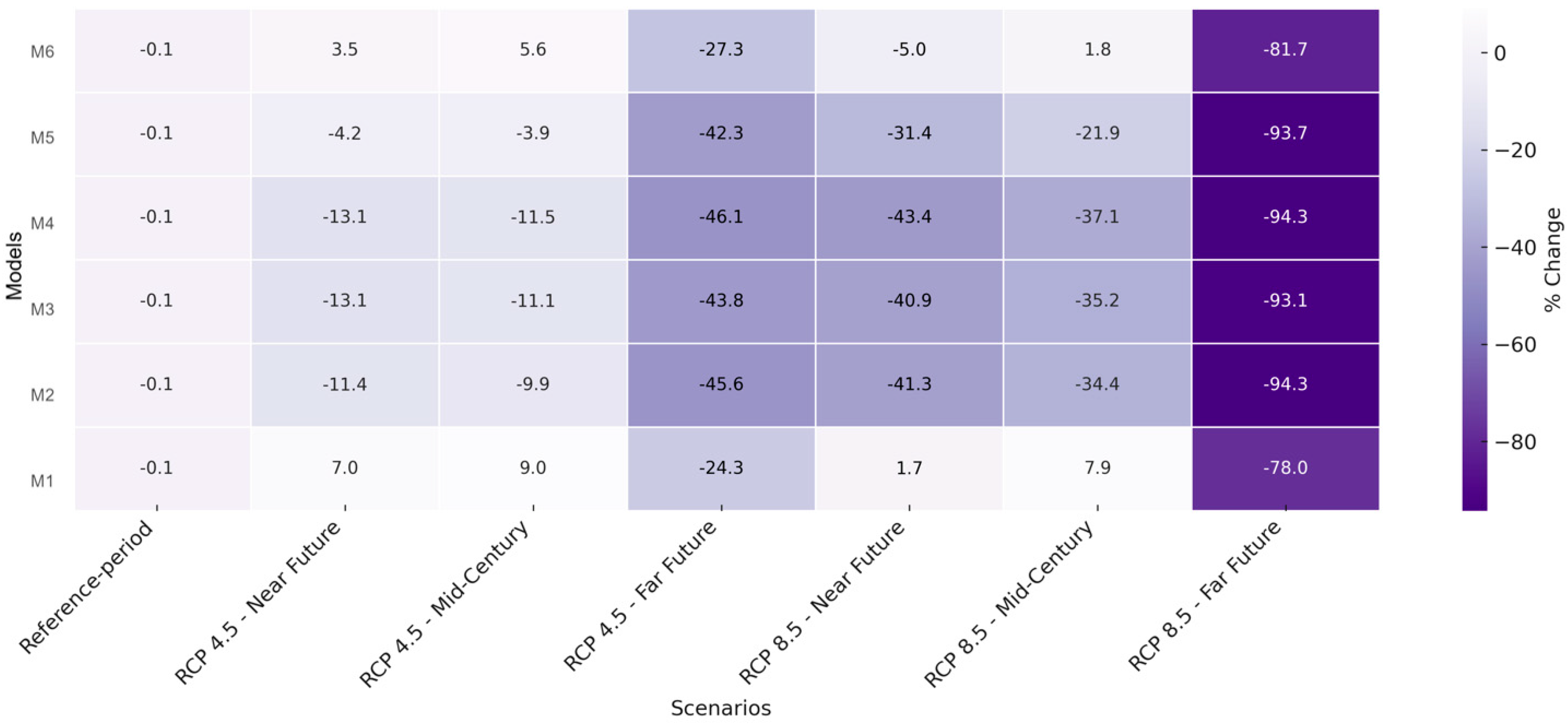
| Model | Reference Period | RCP 4.5 Near | RCP 4.5 Mid | RCP 4.5 Far | RCP 8.5 Near | RCP 8.5 Mid | RCP 8.5 Far |
|---|---|---|---|---|---|---|---|
| M1 | 0.709 ± 0.047 | 0.760 ± 0.080 | 0.538 ± 0.324 | 0.766 ± 0.199 | 0.774 ± 0.082 | 0.722 ± 0.213 | 0.156 ± 0.236 |
| M2 | 0.709 ± 0.047 | 0.629 ± 0.080 | 0.387 ± 0.203 | 0.466 ± 0.164 | 0.639 ± 0.089 | 0.417 ± 0.167 | 0.040 ± 0.085 |
| M3 | 0.709 ± 0.047 | 0.617 ± 0.072 | 0.399 ± 0.177 | 0.460 ± 0.152 | 0.631 ± 0.084 | 0.419 ± 0.155 | 0.049 ± 0.087 |
| M4 | 0.709 ± 0.047 | 0.617 ± 0.077 | 0.382 ± 0.183 | 0.446 ± 0.157 | 0.629 ± 0.088 | 0.402 ± 0.159 | 0.040 ± 0.080 |
| M5 | 0.709 ± 0.047 | 0.680 ± 0.101 | 0.410 ± 0.280 | 0.554 ± 0.197 | 0.682 ± 0.105 | 0.487 ± 0.201 | 0.054 ± 0.115 |
| M6 | 0.709 ± 0.047 | 0.735 ± 0.080 | 0.516 ± 0.308 | 0.723 ± 0.194 | 0.749 ± 0.083 | 0.675 ± 0.206 | 0.130 ± 0.207 |
| Model | RCP 4.5 Near | RCP 4.5 Mid | RCP 4.5 Far | RCP 8.5 Near | RCP 8.5 Mid | RCP 8.5 Far |
|---|---|---|---|---|---|---|
| M1 | +7.0% | −24.3% | +7.9% | +9.0% | +1.7% | −78.0% |
| M2 | −11.4% | −45.6% | −34.4% | −9.9% | −41.3% | −94.3% |
| M3 | −13.1% | −43.8% | −35.2% | −11.1% | −40.9% | −93.1% |
| M4 | −13.1% | −46.1% | −37.1% | −11.5% | −43.4% | −94.3% |
| M5 | −4.2% | −42.3% | −21.9% | −3.9% | −31.4% | −93.7% |
| M6 | +3.5% | –27.3% | +1.8% | +5.6% | +5.0% | –81.7% |
| Method | AUC | COR | TSS | Deviance |
|---|---|---|---|---|
| Bioclim | 0.92 | 0.38 | 0.84 | 0.03 |
| GLM | 0.98 | 0.24 | 0.95 | 0.03 |
| BRT | 0.96 | 0.25 | 0.91 | 0.04 |
| RF | 0.98 | 0.15 | 0.95 | 0.04 |
| Maxent | 0.99 | 0.38 | 0.96 | 0.08 |
Disclaimer/Publisher’s Note: The statements, opinions and data contained in all publications are solely those of the individual author(s) and contributor(s) and not of MDPI and/or the editor(s). MDPI and/or the editor(s) disclaim responsibility for any injury to people or property resulting from any ideas, methods, instructions or products referred to in the content. |
© 2025 by the authors. Licensee MDPI, Basel, Switzerland. This article is an open access article distributed under the terms and conditions of the Creative Commons Attribution (CC BY) license (https://creativecommons.org/licenses/by/4.0/).
Share and Cite
Carlini, B.; Velázquez, J.; Gülçin, D.; Rincón, V.; Lucini, C.; Çiçek, K. The Impact of Climate Change on the Sustainability of PGI Legume Cultivation: A Case Study from Spain. Agriculture 2025, 15, 1628. https://doi.org/10.3390/agriculture15151628
Carlini B, Velázquez J, Gülçin D, Rincón V, Lucini C, Çiçek K. The Impact of Climate Change on the Sustainability of PGI Legume Cultivation: A Case Study from Spain. Agriculture. 2025; 15(15):1628. https://doi.org/10.3390/agriculture15151628
Chicago/Turabian StyleCarlini, Betty, Javier Velázquez, Derya Gülçin, Víctor Rincón, Cristina Lucini, and Kerim Çiçek. 2025. "The Impact of Climate Change on the Sustainability of PGI Legume Cultivation: A Case Study from Spain" Agriculture 15, no. 15: 1628. https://doi.org/10.3390/agriculture15151628
APA StyleCarlini, B., Velázquez, J., Gülçin, D., Rincón, V., Lucini, C., & Çiçek, K. (2025). The Impact of Climate Change on the Sustainability of PGI Legume Cultivation: A Case Study from Spain. Agriculture, 15(15), 1628. https://doi.org/10.3390/agriculture15151628