Machine Learning-Based Comparative Analysis on Direct and Indirect Mapping of Soil Texture Types Through Soil Particle Size Fractions Using Multi-Source Remote Sensing

Abstract

Soil texture, defined by the proportions of sand, silt, and clay particles in the soil, is one of the most essential physical properties of soil. High-resolution soil texture data can provide critical parameter support for soil hydrological modeling, agricultural production management, and ecosystem assessment. In digital soil mapping, previous studies often predicted the sand, silt, and clay contents in soil and then indirectly calculated soil texture. Currently, approaches that directly map soil texture by classification modeling are gaining increasing attention due to the decreased error from data conversion, but few studies have systematically compared these two methods yet. In this study, we comprehensively assessed the performance of direct and indirect predicting soil texture using four machine learning algorithms (e.g., extreme gradient boosting, random forest, gradient boosting decision tree, and extremely randomized tree) with 190 covariates from the Digital Elevation Model, Sentinel-1/2 satellite images, and classification maps and generated a 10 m resolution soil texture map based on 405 topsoil (0–20 cm) sample data collected in Suichuan County, China. The results showed that compared with indirect predictions, direct predictions improved overall accuracy (OA) by 20.57–44.19% and the Kappa coefficient (Kappa) by 0.220–0.402. Among the models used, the XGB model achieved the highest accuracy (OA: 0.948; Kappa: 0.931) and the lowest uncertainty (confusion index: 0.052). The direct prediction map (nine classes recorded) exhibited more detailed and diverse spatial distribution patterns than the indirect prediction map (six classes recorded), aligning better with the actual environment. Based on accuracy validation and spatial distribution, the performance of the XGB model was best during direct prediction. The Shapley additive explanation from the XGB model revealed that the normalized height and stream power indices were the most significant factors driving the soil texture in the study area. Our results provide a reference for future studies on soil texture mapping using machine learning models.

1. Introduction

Soil texture, characterized by the quantitative distribution of particle size fractions (PSFs) and classified by the texture triangle, constitutes a fundamental physical property in soil science. It governs soil buffering capacity [1], carbon cycling [2], water dynamics, and erodibility [3] and is closely related to climate, ecology, hydrological modeling, and soil pollution control [4,5]. Soil texture distribution can be applied across multiple domains, including cultivated land quality assessment and crop suitability evaluation [6,7]. The spatial mapping of soil texture is important for soil surveys, environmental sustainability, and food security [8].

Traditional soil mapping methods relying on ground surveys are time-consuming, labor-intensive, and highly subjective [9]. Therefore, an efficient and robust approach is required to obtain soil texture information. Digital soil mapping (DSM) has recently emerged as a significant method that can be used to acquire spatial distribution information on various soil attributes [10]. It is primarily based on a soil-landscape model, which combines different environmental covariates and applies spatial analysis and statistical methods to predict soil attributes. DSM represents the spatial continuity and variability of soil attributes using a raster format [11]. Climate, stratigraphic, and topographic maps are crucial data sources for soil attribute mapping, and their effectiveness has been confirmed in previous studies [8,12,13]. The application of remote sensing imagery has gained widespread popularity in recent studies. Optical remote sensing imagery has been extensively utilized in soil texture prediction [4,14]. Although vegetation cover affects the acquisition of soil spectral signals, the correlation between soil and vegetation has led to the incorporation of vegetation indices into soil attribute modeling for vegetated areas [15,16,17]. In contrast, only limited research has been conducted using radar imagery for soil texture prediction in vegetated areas [18,19]. The possibility of using radar remote sensing data to retrieve vegetation characteristics has been demonstrated in previous studies [20,21]. Moreover, several studies have shown that optical and radar remote sensing data complement each other in monitoring vegetation properties [22]. Therefore, the potential utility of multi-source remote sensing data in soil texture modeling requires urgent investigation.

In DSM, soil texture can be directly predicted by using classification modeling methods [23,24,25] or indirectly predicted by first predicting sand, silt, and clay contents in the soil and then calculating soil texture [26,27,28]. The soil PSFs are compositional data. In the indirect prediction of soil textures, the soil PSFs have to be nonnegative and sum to 1 (100%) [29,30]. The closure effect leads to spurious correlations, which interfere with statistical analysis and model predictions [31]. Therefore, scholars have proposed various transformation methods for compositional data to minimize errors [32], and symmetric log-ratio (SLR) transformation has proved to be the best transformation method [33,34]. In contrast, the direct prediction method excludes this step, theoretically reducing the error. Currently, few studies systematically compare direct and indirect methods, which typically either employ single models or generate sub-10 m resolution maps. For instance, Mirzaei et al. [35] only through the random forest classification model successfully mapped soil texture distribution in the Kuhdasht region in western Iran with a 30 m resolution by using Landsat-8, Sentinel-2, and DEM covariates. In addition, they merely visualized the model’s built-in importance ranking without delving into the driving factors of soil texture. Various modeling approaches, including linear regression equations, geostatistical methods, and machine learning algorithms, have been successfully applied to predict soil attributes [36,37]. Among these approaches, machine learning algorithms are favored by researchers because they can handle the complex nonlinear relationships between soils and environmental factors. The machine learning algorithms include random forest (RF) [38], gradient boosting decision tree (GBDT) [39], extremely randomized tree (ETR) [40], and extreme gradient boosting (XGB) [41]. Due to the limited studies on the comparison of direct and indirect methods for soil texture prediction, it remains unclear which of these two approaches will be conducive to its estimation and which extent of prediction performance we can achieve using optimal machine learning models.

To fill the aforementioned knowledge gap, the objectives of our study are threefold: (1) explore the effectiveness of multi-source remote sensing data for soil texture prediction; (2) compare the performance of direct and indirect approaches for soil texture prediction using multiple machine learning algorithms; and (3) generate a soil texture map with a 10 m resolution and clarify the driving factors. The study integrated multi-source remote sensing data, systematically compared the direct and indirect prediction approaches of four models, broke through the limitations of a single data source or modeling method, and provided a replicable methodological framework for soil texture mapping.

2. Materials and Methods

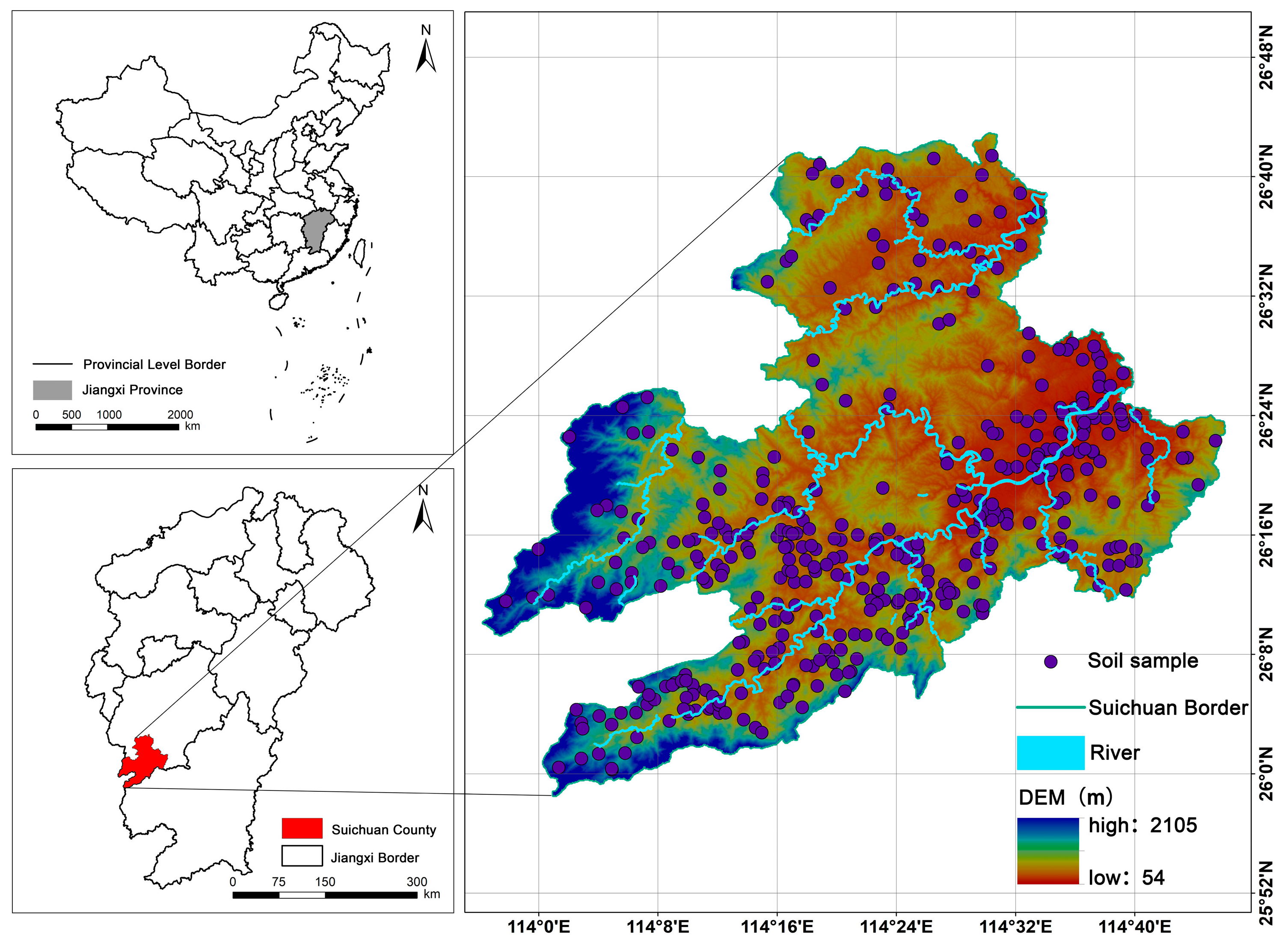
2.1. Study Area

Suichuan County (25°28′32″–26°42′55″ N, 113°56′51″–114°45′45″ E), with an area of 3144.17 km², is located to the southwest of Ji’an City, Jiangxi Province (Figure 1). Influenced by its natural environment, the county is predominantly mountainous, with higher altitudes in the southwest region and lower altitudes in the northeast region. The southwest region of the county is dominated by the main ridge of Mount Wanyang, the highest peak in Jiangxi Province, which is the ‘roof ridge’ of Suichuan. The county features a well-developed water system, with the Suichuan River and Shisui River, both primary tributaries of the Gan River. These rivers flow towards the northeast of Suichuan County through Wan’an County before converging into the Gan River. Suichuan County features a humid monsoon climate with abundant light and four demarcated seasons. It has sufficient heat and rainfall, with an annual mean temperature of 19.1 °C and an annual mean rainfall of 1525.5 mm.

The research framework is shown in Figure 2. To obtain fine and accurate soil texture maps, we integrated multi-source data, including the Digital Elevation Model, Sentinel-1/2 satellite images, and classification maps. Soil texture is predicted by combining two modeling strategies (e.g., direct and indirect prediction), and four machine learning models (e.g., GBDT, XGB, RF, and ETR). Ultimately, Shapley Additive Interpretation was used to analyze the driving factors.

2.2. Soil Sampling and Laboratory Analysis

Based on the stratification of soil types, land use types, and DEM in Suichuan County, 405 sampling points were collected from areas excluding reservoirs and ravines in December 2023. In order to mitigate noise interference in the soil samples, the five-point mixing sampling method was applied in each stratified random representative plot. The locations of the sampling points were recorded using a global positioning system (GPS), along with comprehensive details on parent material, landform, and other associated environmental conditions. Due to the complicated soil types in the south and east of the country, there were more soil sampling points. In contrast, fewer samples were collected in the central and northern regions because of the relatively similar soil types. The final laboratory analysis was based on the average of the 5 topsoil (0–20 cm) samples collected from each plot. The soil samples were pre-processed in a laboratory through natural air drying, debris removal, and sieving. Approximately 30 g of each sample was used to measure soil PSFs, analyzed by a Malvern Panalytical Mastersizer 2000 laser (Spectris plc., Malvern, UK) diffraction particle size analyzer (the mean error was below 3%) [42].

2.3. Environmental Covariates

The climate covariates, relief covariates, remote sensing covariates, and classification maps including parent material (PM), stratigraphic (SG), and land use (LULC) are related to the soil texture distribution [43]. Since climatic conditions are consistent across a country, we did not consider them. We processed 187 continuous covariates (

Table 1. List of environmental covariates included in the database.

Type	Covariate *	Abbreviation	Scale	Remark
Relief	Elevation	DEM	12.5 m	https://search.asf.alaska.edu/ (accessed on 9 October 2024)
	Slope	SLP		Extracted from DEM data
	Aspect	APT
	Terrain Wetness Index	TWI
	Curvature	Curv
	Plan Curvature	PLC
	Profile Curvature	PRC
	Topographic Position Index	TPI
	Terrain Ruggedness Index	TRI
	Multi-resolution Index of Ridge Top Flatness	MRRTF
	Multi-resolution Index of Valley Bottom Flatness	MRVBF
	Stream Power Index	SPI
	Mid-Slope Position	MSP
	Standardized Height	SDH
	Normalized Height	NH
	Valley Depth	VD
	Slope Height	SPH
	Multi-scale Topographic Position Index	MTPI
	Slope Length and Steepness Factor	LSF
Sentinel-1	Vertical-Vertical	VV	10 m	Extracted from Sentinel-1 data
	Vertical-Horizontal	VH
	Cross Ratio	CR		${\displaystyle \frac{VH}{VV}}$
	Radar Vegetation Index	RVI		$4\times {\displaystyle \frac{VH}{VV+VH}}$
Sentinel-2	Plant Red-Edge Band 1	B5		Extracted from Sentinel-2 data
	Plant Red-Edge Band 2	B6
	Plant Red-Edge Band 3	B7
	Normalized Difference Vegetation Index	NDVI		${\displaystyle \frac{B8-B4}{B8+B4}}$
	Enhanced Vegetation Index	EVI		$2.5\times {\displaystyle \frac{B8-B4}{B8+6\times B4-7.5\times B2+1}}$
	Normalized Difference Water Index	NDWI		${\displaystyle \frac{B3-B8}{B3+B8}}$
	Normalized Difference Moisture Index	NDMI		${\displaystyle \frac{B8-B11}{B8+B11}}$
	Inverted Red-Edge Chlorophyll Index	IRECI		$\left(B7-B4\right)\times {\displaystyle \frac{B6}{B5}}$
	Bare Soil Index	BSI		${\displaystyle \frac{\left(B11+B4\right)-\left(B8+B2\right)}{\left(B11+B4\right)+\left(B8+B2\right)}}$
	Soil Adjusted Vegetation Index	SAVI		${\displaystyle \frac{1.5\times \left(B8-B4\right)}{B8+B4+0.5}}$

* The interpretation of some covariates is in Supplementary Table S2.

) and 3 classification maps at a resolution of 10 m. The code of classification maps is in Supplementary Table S1. Owing to the multi-collinearity of the covariates, recursive feature elimination (RFE) [44] can be used to screen the covariates before model construction, selecting the covariate combination with the highest accuracy (e.g., F1 score or R²) as the final model input.

2.3.1. Relief

DEM data were sourced from the NASA Earth science data website https://search.asf.alaska.edu/ (accessed on 9 October 2024), and 19 relief covariates including slope (SLP), aspect (APT), planar curvature (PLC), profile curvature (PRC), terrain wetness index (TWI), and terrain position index (TPI) were extracted using SAGA GIS 7.8.2 software.

2.3.2. Remote Sensing Images

Sentinel-1 and Sentinel-2 images were obtained using the Google Earth Engine, a cloud computing platform, for cloud removal and the monthly average backscattering coefficients for the vertical–vertical (VV) and vertical–horizontal (VH) polarizations [41,45], radar vegetation index (RVI), and cross-polarization ratio (CR) [46,47] of Suichuan County, calculated for 2023. Optical remote sensing covariates include the monthly average plant red-edge 1/2/3 bands (B5, B6, and B7) [48], normalized difference vegetation index (NDVI) [49], enhanced vegetation index (EVI) [39], normalized difference water index (NDWI) [50], normalized difference moisture index (NDMI) [51]), inverted red-edge chlorophyll index (IRECI) [39], bare soil index (BSI) [24], and soil-adjusted vegetation index (SAVI) [52].

2.4. Predictive Modelling Approaches

Two approaches were employed to produce soil texture maps: the direct classification prediction of soil texture and indirect prediction by initially estimating sand, silt, and clay particles and then calculating the relevant texture. The dataset was divided into training (80%) and testing (20%) subsets.

2.4.1. Direct Prediction Approach

In the direct prediction approach, we trained four models—GBDT [53], RF [54], XGB [55], and ETR [56] (Supplementary S1.1). These have been proven effective in handling complex nonlinear relationships and are robust to overfitting [57]. Stratified by soil texture class, the dataset was divided into training (80%) and test (20%) subsets via random sampling in each layer. The models were then trained on the training subset using 30 iterations of 10-fold cross-validation, with Bayesian optimization [58] employed to determine the optimal hyperparameters robustly and efficiently in a way that minimizes the evaluation cost. The final model obtained using repeated cross-validation was evaluated on the testing data.

2.4.2. Indirect Prediction Approach

In the indirect prediction approach, soil PSFs were simulated using identical machine learning approaches. As compositional data that total 100%, the soil PSFs are typically modeled using SLR transformation [32]. The SLR-transformed data were used to train the models. The models were trained through 30 iterations of 10-fold cross-validation using the identical 80% training subset applied to identify the optimal hyperparameters for each model. The optimal models were assessed using the testing subset on back-transformed values of soil PSFs. The initial maps from model outputs were then back-transformed using inverse SLR to generate the soil PSF maps. Finally, the maps were calculated into texture maps based on soil texture classification criteria.

The SLR transformation formula is as follows:

$$Z_{ij}^{\prime }=\ln {\displaystyle \frac{Z_{ij}+{\delta }_j}{{\left({\prod }_{j=1}^D{Z}_{ij}+{\delta }_j\right)}^{1/D}}}$$

(1)

The back-converted formula is as follows:

$$Z_{ij}=\ln \left({\displaystyle \frac{\exp Z_{ij}^{\prime }}{{\displaystyle {\sum }_{j=1}^D\exp Z_{ij}^{\prime }}}}-{\displaystyle \frac{{\delta }_j}{1+{\displaystyle {\sum }_{j=1}^D{\delta }_j}}}\right)\left(1+{\displaystyle \sum _{j=1}^D{\delta }_j}\right)$$

(2)

where $Z_{ij}$ is the relative content (%) of the i-th sample point and j-th particle size; $Z_{ij}^{\prime }$ is the conversion value of the content of the i-th sample point and j-th particle size; D denotes the dimension of component data; and D = 3; ${\delta }_j$ is a constant, taking half of the minimum content of the j-th particle, excluding 0.

2.5. Evaluation of Feature Importance

Shapley additive explanation (SHAP) provides a unified framework for interpreting complex black-box models [59]. It bridges Shapley values from game theory with local explanations to assess the marginal contribution of each input feature to individual predictions. It can be expressed using Equation (3).

$$g(z^{\prime })={\varphi }_0+{\displaystyle \sum _{i=1}^M{\varphi }_i{z_i}^{\prime }}$$

(3)

where $z^{\prime }\in {\{0,1\}}^M$ denotes whether there are feature variables; M is the number of feature variables; ${\varphi }_0$ is constant when all inputs are absent; and ${\varphi }_i$ is the marginal contribution of variable i, also known as the Shapley value of i. Python 3.10 was used in the study to invoke the SHAP packet to quantify the importance of each feature variable in the models.

2.6. Validation of Soil Texture Classification

2.6.1. Evaluation Indicators for Soil Texture Classification

The hyperparameter tuning of the model was performed using 10-fold cross-validation and Bayesian optimization. We took the mean value (repeated 30 times) of the model to obtain a stable performance. The selected evaluation indicators were the overall accuracy (OA), precision, recall, F1 score, and Kappa coefficient (Kappa) [60], as shown in Equations (4)–(8):

$$\mathrm{OA}={\displaystyle \frac{\mathrm{TP}+\mathrm{TN}}{\mathrm{TP}+\mathrm{TN}+\mathrm{FP}+\mathrm{FN}}}$$

(4)

$$\mathrm{precision}={\displaystyle \frac{\mathrm{TP}}{\mathrm{TP}+\mathrm{FP}}}$$

(5)

$$\mathrm{recall}={\displaystyle \frac{\mathrm{TP}}{\mathrm{TP}+\mathrm{FN}}}$$

(6)

$$\mathrm{F}1\mathrm{score}={\displaystyle \frac{2\mathrm{Precision}\times \mathrm{Recall}}{\mathrm{Precision}+\mathrm{Recall}}}$$

(7)

$$\mathrm{Kappa}={\displaystyle \frac{{\mathrm{P}}_{\mathrm{o}}{-\mathrm{P}}_{\mathrm{e}}}{1-{\mathrm{P}}_{\mathrm{e}}}}$$

(8)

where TP, TN, FP, and FN are true positive, true negative, false positive, and false negative, respectively. F1 score is the weighted average of precision and recall; P_o is the probability of observed agreement; and P_e is the probability of agreement when two classes are unconditionally independent. OA evaluates the overall performance of the model, while Kappa considers random consistency to assess the actual classification ability of the model. The F1 score is the harmonic mean of accuracy and recall, which can better measure the performance of the model on minority classes.

The confusion index (COI), proposed by Burrough et al. [61], was applied to quantify the uncertainties in machine learning classification models. It can be expressed using Equation (9).

$$COI={\displaystyle \frac{{\displaystyle {\sum }_{i=1}^n\left[1-\left(P_{\max ,i}-P_{\sec \max ,i}\right)\right]}}{n}}$$

(9)

where P_max,i is the probability of the most probable class for soil sampling point i, and P_secmax,i is the probability of the second most probable class for soil sampling point i. The COI values vary from 0 to 1, of which larger values denote higher uncertainty.

2.6.2. Evaluation Indicators for Soil PSF Prediction

The performance of the four machine learning models was evaluated by calculating the mean absolute error (MAE), root mean square error (RMSE), and coefficient of determination (R²) between the observed and predicted values at the validation sample points [62]. Equations (10)–(12) are as follows:

$$RMSE=\sqrt{{\displaystyle \frac{{\displaystyle {\sum }_{i=1}^n{\left[z\left(x_i\right)-Z\left(x_i\right)\right]}^2}}{n}}}$$

(10)

$$MAE={\displaystyle \frac{1}{n}}{\displaystyle \sum _{i=1}^n\left|\mathrm{z}(x_i)-Z(x_i)\right|}$$

(11)

$$R^2=1-{\displaystyle \frac{{\displaystyle {\sum }_{i=1}^n{\left[z\left(x_i\right)-Z\left(x_i\right)\right]}^2}}{{\displaystyle {\sum }_{i=1}^n{\left[Z\left(x_i\right)-{}^{-}Z\left(x_i\right)\right]}^2}}}$$

(12)

where n is the number of sample points used in the validation set; $z\left(x_i\right)$ is the predicted value at sample point i; $Z\left(x_i\right)$ is the observed value at sample point i; and ${}^{-}Z\left(x_i\right)$ is the average of the observed values at sample points 1 to i.

The uncertainty of each model was assessed by calculating the standard deviation (SD) of the results of 30 runs, as described by Zhou et al. [63].

3. Results

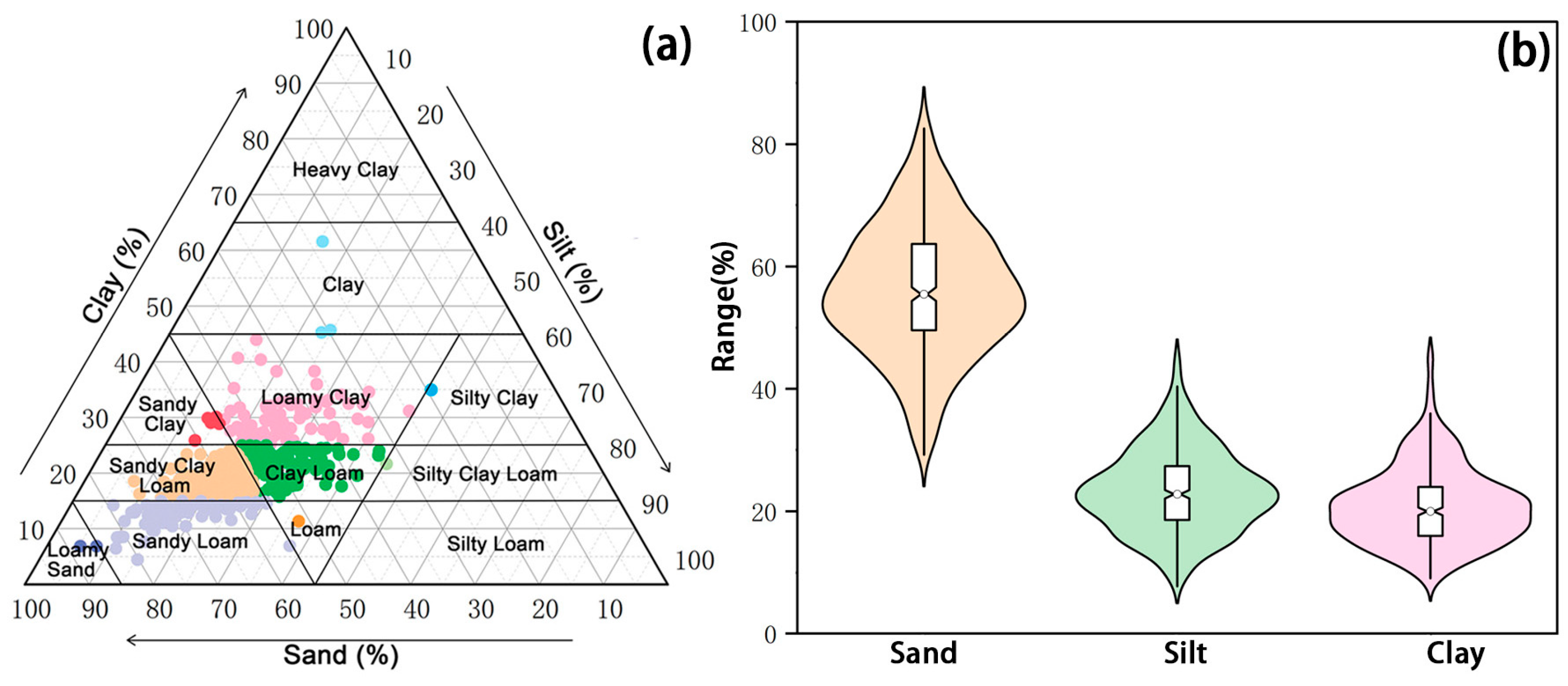
3.1. Descriptive Statistics of the Soil Samples

Suichuan County has nine types of soil textures, and the most common types are sandy clay loam and clay loam (Figure 3a). The descriptive statistics of soil PSFs indicate that the County has a high sand content, with an average of 56.10%, and a low clay content, with an average of 20.86% (Figure 3b). In terms of the variation coefficient, the sand content is substantially lower than either the clay or silt content. Soil PSF distribution generally exhibits skewness and kurtosis values consistent with a normal distribution (

Table 2. Descriptive statistics of soil sample points.

Property	Unit	Min	Max	Mean	Standard Deviation	Skewness	Kurtosis	%Variation Coefficient
Sand	%	24.60	85.40	56.10	10.72	0.05	2.80	19.11
Silt	%	6.60	45.70	23.30	6.79	0.39	3.05	29.14
Clay	%	6.90	45.70	20.86	6.38	−0.10	2.97	30.58

).

The covariate combination for directly and indirectly predicting soil texture was obtained based on the optimal model performance of the RFE (

Table 3. Optimal factor combinations for soil texture prediction identified using the RFE model.

Property	Type	Variable List	Number	Evaluation Indicators
Soil Texture	Relief	VD—NH—SPI—MSP	4	F1 score = 0.708
	Sentinel-1	RVI_07	1
	Sentinel-2	NDVI_07—NDVI_02	2
	classification maps	PM	1
Sand	Relief	VD—SPI—NH	3	R2 = 0.694
	Sentinel-1	CR_04—RVI_10—CR_08—RVI_01—RVI_07	5
	Sentinel-2	NDVI_07—NDVI_05—NDVI_08	3
	classification maps	PM—SG	2
Silt	Relief	SPI—SPH—VD—MSP	4	R2 = 0.727
	Sentinel-1	CR_10—CR_04—RVI_07	3
	Sentinel-2	NDVI_09—NDVI_02—NDVI_10	3
	classification maps	SG—PM	3
Clay	Relief	NH—VD—SPI—APT	4	R2 = 0.645
	Sentinel-1	CR_08—RVI_01	2
	Sentinel-2	NDVI_07—NDVI_10—NDVI_02—NDVI_05	4
	classification maps	PM—SG	2

). Of the 190 covariates, 8 covariates were retained in the RFE for the soil texture (F1 score: 0.708); these included 4, 1, 2, and 1 covariates related to the relief, Sentinel-1, Sentinel-2, and classification maps, respectively. As for the sand particles, the RFE (R² = 0.694) retained 13 covariates, with 3, 5, 3, and 2 covariates related to the relief, Sentinel-1, Sentinel-2, and classification maps, respectively. In the case of the silt particles, the RFE (R² = 0.727) retained 13 covariates related to the relief, Sentinel-1, Sentinel-2, and classification maps. Regarding the clay particles, 12 covariates were retained in the RFE (R² = 0.645), including 4, 2, 4, and 2 covariates related to the relief, Sentinel-1, Sentinel-2, and classification maps, respectively.

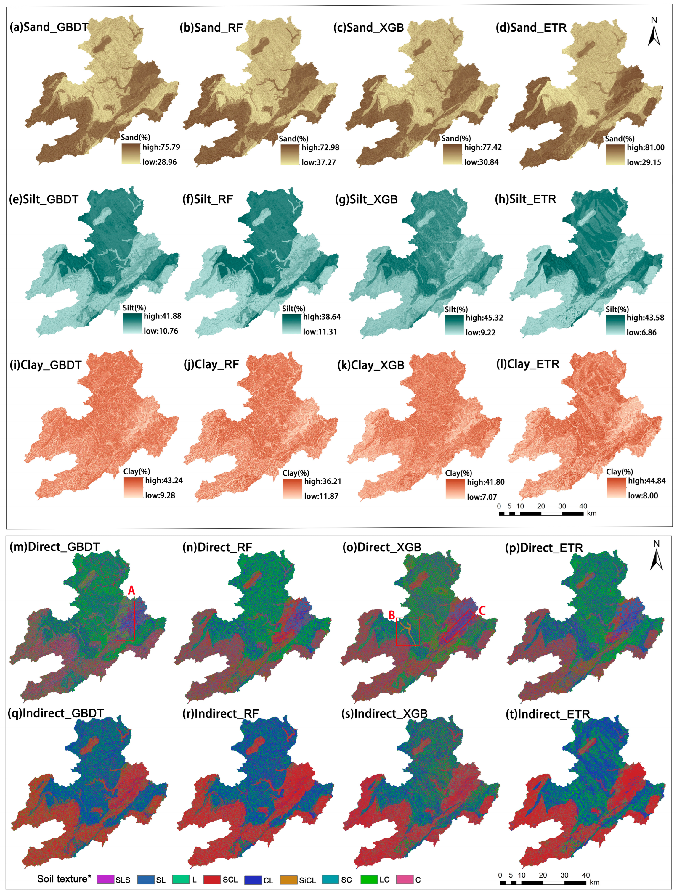
3.2. Direct Prediction of the Soil Textures

With the optimal covariate combination (Table 3), the validation indicators obtained in the direct prediction of soil textures using different algorithms varied (

Table 4. Soil texture prediction accuracies of the different models.

	Models	OA	Kappa	F1 score	Precision	Recall	COI
Direct	GBDT	0.923	0.898	0.854	0.846	0.866	0.077
	XGB	0.948	0.931	0.878	0.880	0.877	0.052
	RF	0.943	0.924	0.876	0.878	0.875	0.057
	ETR	0.938	0.918	0.874	0.876	0.873	0.062
Indirect	GBDT	0.728	0.630	0.315	0.334	0.311	0.272
	XGB	0.662	0.541	0.348	0.355	0.382	0.338
	RF	0.654	0.522	0.266	0.324	0.270	0.346
	ETR	0.778	0.698	0.347	0.359	0.350	0.222

). XGB produced the highest OA of 0.948 followed by RF (0.943), GBDT (0.923), and ETR (0.938). The XGB also produced the highest Kappa coefficient of 0.931, with RF, ETR, and GBDT producing progressively lower values. The F1 score obtained using XGB was 0.878 (precision: 0.880, recall: 0.877) demonstrating excellent discrimination for both positive and negative class samples. The XGB yielded the lowest COI of 0.052, while the GBDT yielded a COI of 0.077, indicating greater uncertainty than XGB.

The soil texture distributions obtained using different models are consistent but exhibit local differences (Figure 4). The soil textures in the northern and central regions are mainly loamy clay, while the soil texture in the southwest region is mainly sandy clay loam. The PM in area A in Figure 4m is of various types and mainly red sandstone weathering material, with the main lithology comprising complex conglomerate and sandstone conglomerate. The soil texture in the area typically varies from sandy loam to sandy clay loam. Therefore, the soil texture predicted using GBDT is not consistent with the actual soil texture. Although the PM of area B shown in Figure 4o is Quaternary red clay, the lithology of the area comprises silty slate, while the soil texture of the area is often silty clay loam. Therefore, the soil texture predicted using XGB is in line with the actual soil texture of the area. This also confirms that XGB effectively reduces the model’s sensitivity to noise through an improved loss function and regularization design. Therefore, it achieves more reliable predictions than GBDT in areas A and B where the parent materials are complex. Based on index verification and distribution authenticity, XGB was found to be the model best for directly predicting soil textures. Its map shows mainly loamy clay (33.80%) and sandy clay loam (23.09%), concentrated in the central and northern regions and the southwest region, respectively.

3.3. Indirect Prediction of the Soil Textures

The indirect prediction of the soil textures using the optimal covariate combination (Table 3) showed that the ETR model best predicted the sand content, with the lowest RMSE (4.973%) and MAE (2.107%) and the highest R² (0.784) (Supplementary Table S3). Meanwhile, the ETR model will be the most suitable model for predicting the silt and clay contents in soil. Moreover, the ETR model yielded the lowest uncertainties (SD: 4.975, 3.020, and 3.209) for soil PSFs (Supplementary Table S3).

Referring to the Co-kriging prediction map (Supplementary Figure S1), the spatial distributions of the soil PSFs yielded by different models are similar (Figure 4). The areas with high sand contents are mainly concentrated in the southwestern and eastern regions of the county, while its central and northern regions have low sand contents. The spatial distribution pattern of silt is opposite to that of sand. The spatial heterogeneity of clay is slightly weaker than that of silt, but its pattern is consistent with that of silt. Moreover, the prediction map produced by the ETR model is closer to the original data range than the maps produced by other models. Thus, the ETR model can cover the data distribution of the soil PSFs (the difference between the predicted extreme values and the original extreme values is relatively small). The ETR model performed best when converting pixel-level information into soil texture maps (OA: 0.778; Kappa: 0.698; COI: 0.222). Furthermore, the soil texture map produced by the ETR model shows more substantial spatial heterogeneity than that produced by any of the other models. Thus, the ETR model is the best model for the indirect prediction of soil textures.

3.4. Comparison of the Direct and Indirect Soil Texture Predictions

All models performed well in the direct prediction of soil textures, with a high OA and low COI (Table 4) (e.g., the XGB model yielded an OA of 0.948, a Kappa of 0.931, and a COI of 0.052). However, the indirect prediction indicators were substantially worse than the direct prediction indicators. The total RMSE of the indirect prediction was 11.210–13.629% (Supplementary Table S3), and there was a contraction in the predicted range (Figure 4a–i). Consequently, even the ETR yielded the highest OA of 0.778 in indirect prediction, which was lower than that yielded in direct prediction. The F1 score and other indicators also displayed similar disparities, with the direct prediction models better balancing precision and recall compared with the indirect prediction models. Overall, compared with indirect prediction, the OA of direct prediction increased by 20.57% to 44.19%, and the Kappa increased by 0.220 to 0.402, making it more accurate and effective in identifying soil texture. We verified this finding by Fisher’s Exact Test (Supplementary Table S4).

The texture distribution patterns produced by Direct_XGB and Indirect_ETR are generally consistent, but localized differences can still be observed (Figure 4o,t). Compared with the Indirect_ETR map (six classes recorded), the Direct_XGB map (nine classes recorded) exhibited more detailed and diverse class divisions, providing richer information. For the central and northern regions of Suichuan County, where the lithology consists of gray–black high-carbon slate and argillaceous slate, Direct_XGB showed a broader distribution of loamy clay and a lower proportion of clay loam than Indirect_ETR, aligning with the actual conditions. In area C, where the PM comprises alluvial deposits of rivers and lakes, and Quaternary red clay, the soil texture would be predominantly clayey. Compared with Indirect_ETR, Direct_XGB reflected this soil texture more accurately because the clay loam proportion it showed was higher than that shown by Indirect_ETR. The southwestern region, with high elevations and PMs comprising weathered acidic crystalline rocks, has a light soil texture. The small proportion of sandy clay loam yielded by Direct_XGB was consistent with the local PM conditions. Thus, the direct prediction of soil textures would be more accurate than the corresponding indirect prediction.

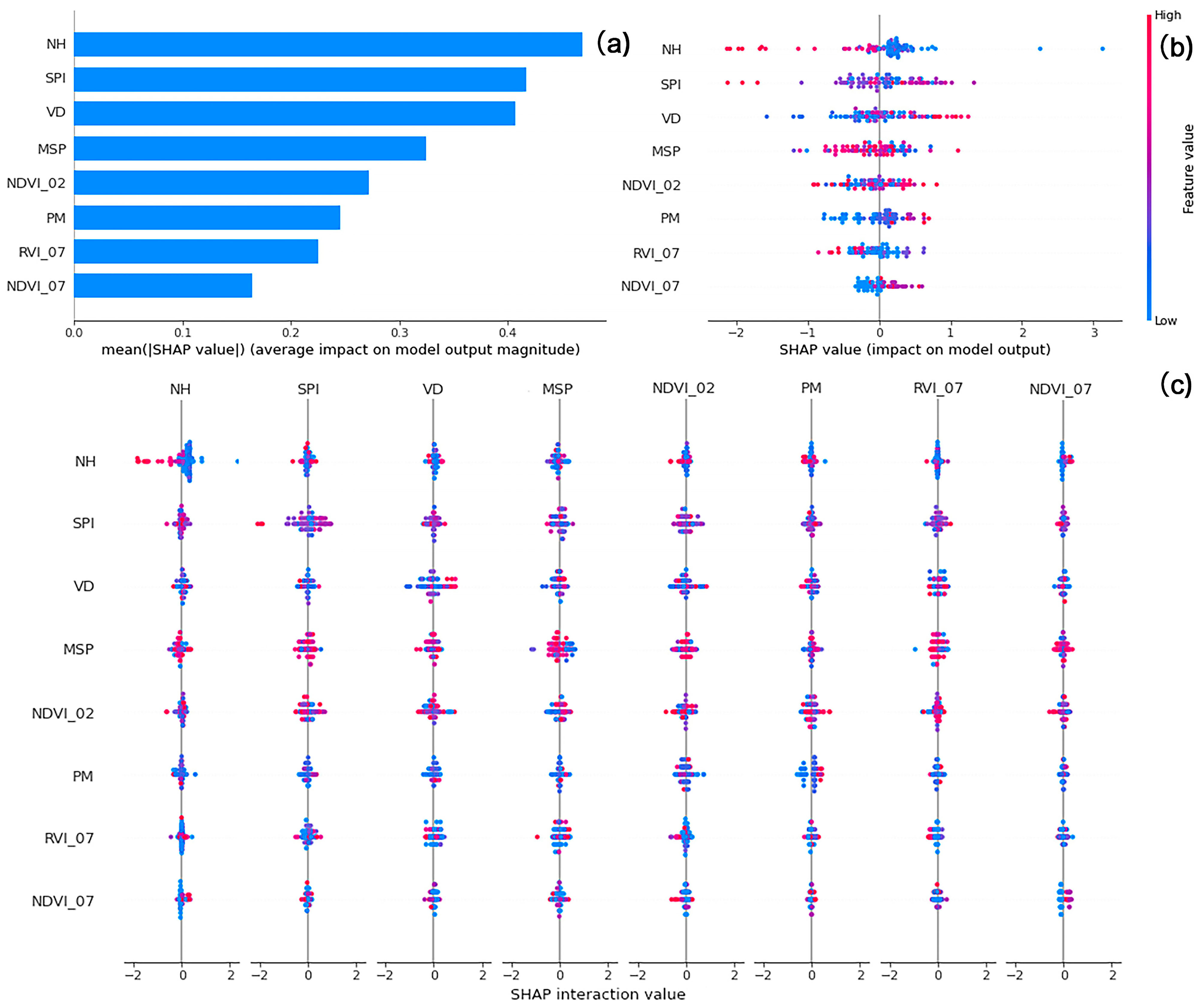
3.5. Interpretable Prediction of Soil Texture

As Figure 5 shows, in direct prediction by XGB, the contributions of various factors were quantified using SHAP. The normalized height (NH), stream power index (SPI), and valley depth (VD) are the three most important driving factors for the mean SHAP absolute values of 0.48, 0.42, and 0.41, respectively (Figure 5a). Among the three driving factors, NH, with a maximum SHAP value of 3.18, was the most influential (Figure 5b). This indicates that the positive impact of a certain low NH value sample on the model had reached the maximum. Compared with other factors, NH and SPI had stronger driving effects, ranging from −2.21 to 3.18 and −2.20 to 1.32, respectively (Figure 5b). The summary chart of the SHAP interaction matrix values (Figure 5c) indicates that the interactions of various driving factors only had a small impact on the soil texture, and the interaction effect of the factors was not therefore considered in predicting the soil textures.

In indirect prediction, among the different driving factors, PM, SPI, and VD have the strongest driving effect on the sand, with SHAP absolute values of 2.75%, 1.83%, and 1.34%, respectively (Figure 6a). PM has a positive effect on sand, while SPI and VD have a negative effect. The maximum impact value of VD reached 6.33% (Figure 6b); PM, SG, and slope height (SPH) are important driving factors for silt, with the SHAP absolute values standing at 2.13%, 1.22%, and 0.88%, respectively (Figure 6c). The influence range of PM and SG was wide, ranging from −3.41% to 5.78% and −3.28% to 4.19%, respectively (Figure 6d). The key driving factors of clay are NH, NDVI_07, and SPI, which had negative, positive, and negative effects, respectively. The maximum SHAP value of NH was 6.62% (Figure 6f). In addition, the interactions of soil PSFs were small, and thus they hardly interfered with soil texture predictions (Supplementary Figure S2). In summary, PM is the most important driving factor for sand and silt, while the relief factors are important driving factors for soil texture class and clay content.

4. Discussion

4.1. Effectiveness of Multi-Source Remote Sensing in Soil Texture Prediction

This study investigated the effectiveness of multi-source remote sensing imagery in predicting soil texture in vegetation-covered areas. The research findings suggest that multi-temporal optical and radar remote sensing covariates in synergy can produce highly accurate soil texture maps. Soil texture affects the availability of soil water retention, aeration, nutrient cycle, and other soil properties, which lead to different vegetation behavioral responses [24]. The heterogeneity in response signals is retrievable through optical and radar satellites and can be characterized by associated environmental covariates derived from them [45].

Previous studies have focused on exploring the potential of optical remote sensing for determining the vegetation–soil correlation [64]. However, those studies have rarely considered the availability of radar data. Radar remote sensing can be used for vegetation phenology extraction, crop identification, and surface biomass inversion [46,47]. Therefore, similar to optical remote sensing, radar remote sensing can characterize vegetation growth and development to infer soil properties. Yang et al. [65] also demonstrated the successful estimation of organic carbon content in soil by analyzing soil–vegetation relationships using multi-temporal Sentinel-1 images. Our study also confirmed this capability of radar remote sensing. After RFE screening, among the 190 initial covariates, the radar covariates can always be retained (Table 3). The SHAP analysis results show that although the overall contribution of radar covariates was lower than that of optical covariates, the contribution of some radar covariates exceeded that of optical covariates (e.g., Figure 5: RVI_07 above NDVI_07). Unlike most studies that use only one single remote sensing data source, such as Landsat series or Sentinel-2 (OA: 0.67–0.85, Kappa: 0.53–0.76) [24,39,52], our study considered the complementarity of different types of satellite sensors, further improving the accuracy of soil texture classification (OA: 0.654–0.948, Kappa: 0.522–0.931). Zhou et al. [63] suggested that radar remote sensing, with its all-weather monitoring capability, can penetrate clouds, fog, and vegetation, and compensate for the shortcomings of optical images (e.g., clouds and fog can block the ground object information, and the atmosphere can cause the distortion of spectral information), thereby bringing new opportunities for soil property monitoring. Therefore, multi-source remote sensing data provide comprehensive vegetation information on soil properties from different dimensions, improving the accuracy of soil texture modeling.

4.2. Comparison of Different Approaches Used in Soil Texture Mapping

The direct prediction of soil textures (OA: 0.923–0.948, Kappa: 0.898–0.931) is better than the indirect prediction (OA: 0.654–0.778, Kappa: 0.522–0.698) concerning all evaluation indicators. Given the different levels of information granularity in the two approaches, indirect prediction approaches, which are based on multiple combinations of soil PSF regression outputs to determine classifications, theoretically generate more classes as a consequence of the substantial number of combinations [66]. However, a notable limitation emerges in predicting soil PSFs, where models exhibit regression towards the mean (e.g., Sand_ETR (Figure 4): 29.15–81.00% vs. original data (Table 2): 24.60–85.40%). This phenomenon is likely attributable to either data noise or spatial heterogeneity. Zhang et al. [42] reported that the contraction prediction towards the center of the texture triangle might prevent the indirect prediction from adding soil texture classes that are not included in the training subset. Thus, this explains that our direct prediction map (nine classes recorded) presents a more detailed and diverse classification than the indirect one (six classes recorded).

Moreover, the feature spatial overlap between adjacent classes results in a marked inadequacy of the model’s discriminative power for adjacent classes. Bhatt et al. [67] found that confusions are generally between adjacent classes. Our study also revealed the same trend in that mismatch tended to originate from the adjacent classes (Supplementary Figure S3). For example, in indirect prediction, 18.02–25.23% of the clay loam was not correctly classified, with most of it classified as sandy clay loam and some of it classified as loamy clay or sandy clay. However, in direct prediction, this type of problem is less frequently encountered. A comparison of the validation indicators of the four different machine learning algorithms revealed that indirect prediction (ETR > GBDT > XGB > RF) did not outperform direct prediction (XGB > RF > ETR > GBDT), which could be due to error accumulation and transmission (total RMSE: 11.210–13.629%) during the conversion of the soil PSF maps into the texture maps [27], leading to increased uncertainty (COI: 0.222–0.346). In direct prediction approaches, XGB demonstrates superior performance in local feature identification within spatial mapping compared to random forest, despite comparable overall accuracies between the two models. This is attributed to XGB’s improved loss function and regularization design, which effectively reduce model sensitivity to noise [55]. Therefore, we took the XGB output of direct prediction as the final soil texture map of Suichuan County. In the soil PSF prediction, the R² range predicted in our study was 0.636–0.802, better than the values obtained by He et al. [68] (R²: 0.53–0.73). The RMSE was also substantially lower than that obtained in other studies [28,69]. Current research mainly focuses on either direct or indirect soil texture prediction approaches in isolation, with a limited systematic comparison between these approaches. Existing comparative studies [35,70] often concentrate on individual machine learning models, particularly random forest algorithms, without comprehensive validation across diverse models. To address this limitation, we applied multiple machine learning models, reducing single-model bias and improving the reliability of our conclusions.

4.3. Interpretability of Soil Texture Spatial Distribution

PM is the key covariate that can be used to distinguish sand particles from silt particles. When the PM is argillaceous rock weathering products, the soil texture prediction suggests an increased number of silt particles and a decreased number of sand particles (Figure 6b: PM has a positive effect; Figure 6d: PM has a negative effect), consistent with the distribution of silt and sand particles in the central and northern regions of Suichuan County (Figure 4). Additionally, in areas where the lithology comprises gray and gray–green meta-feldspar quartz arenaceous sandstone, a high silt content was present, which can be attributed to the influence of chemical, physical, and geological activities [71]. The high SHAP values of SPH and SPI confirm the influence of external factors on silt generation and accumulation (Figure 6c,d).

Although soil texture formation is primarily determined by the PM, as the soil formation progresses, factors such as topography and landform begin to play a key role [72]. Relief factors (SHAP value: 1.64) are the main explanatory variables that can be used for the prediction of soil texture in Suichuan County (Figure 5a). Similar to previous research, Zhou et al. [50], who predicted soil texture in small basins of the Yangtze River, also found relief factors to be the most critical covariates. The NH value (Figure 6f: NH has a negative effect) of the central and northern regions indicates gentle terrain conducive to clay particle deposition; the low SPI value (Figure 6f: SPI has a negative effect) of the regions indicates a weak influence of the water flow on soil particle transportation and sorting, allowing clay and silt particles to remain [73], jointly promoting loamy clay and clay loam formation. The southwestern region of the county has a high altitude and large surface runoff (Figure 6b: SPI has a negative effect), which has a sorting effect on soil particles [74], leading to fine sand particles being carried away. However, the sand content in the southwest is still very high. On the one hand, the coarse sand particles are retained owing to their relatively strong resistance to erosion; on the other hand, it is also due to the positive effect of the PM (Figure 6b). Moreover, seasonal streams, temporary water flows that occur following heavy rain, and other factors could also influence sand particle deposition [75], thereby leading to the formation of sandy loam and sandy clay loam. The low-lying areas of the eastern region are substantially affected by the high SPI value from upstream of the southwest, and most of the fine sand particles brought from upstream are deposited here. Meanwhile, the NH value (Figure 6b: NH has a negative effect) suggests a flat terrain, making it difficult for the fine sand particles to move out, thereby forming sandy loam and sandy clay loam. The model interpretability with regard to clay and soil texture is similar, but the driving force of NDVI_07 is stronger than some relief covariates in the clay particle model. The NDVI_07 value is high in the central and northern regions (Figure 6f: NDVI_07 has a positive effect), where the interaction between organic matter produced by vegetation root exudates, litter decomposition, and soil particles promotes small clay particle aggregation [76]. Although, the NDVI is also high in the southwestern region during July, owing to the high altitude and large slope runoff (Figure 6f: Both SPI and NH have a negative effect), limiting in situ clay particle accumulation (Figure 4i) [74]. From the temporal perspective of covariates, the covariates in July exhibit higher contribution values. This phenomenon can likely be attributed to July being a transitional period from the rainy season to the summer drought, during which vegetation experiences vigorous growth while simultaneously facing water stress. The pronounced dynamics of vegetation indices during this period may enhance their sensitivity to soil properties [77].

This finding will help gain a profound understanding of the complexities associated with soil formation, providing theoretical support for precise soil management and scientific and efficient soil resource management by considering multiple factors. For example, superimposing NH and SPI can accurately identify erosion-prone areas (high SPI+ medium/high NH). The areas are prioritized for contour farming, vegetation buffer zones, etc., while light-texture areas (high NH + low/medium SPI) should avoid excessive farming to control the risk of land degradation.

4.4. Limitations and Deficiencies

Several limitations in soil texture prediction are mainly reflected in aspects such as sample size and data transformation. Different sample sizes can affect the performance of machine learning models [78], but as the sample size increases, its marginal effect can lead to the model accuracy reaching the threshold. It is worth an in-depth exploration to make predictions at different sample sizes to discover the optimal size. In addition, we adopted SLR transformation to process the component data. Although the method has been verified as the best by predecessors [33,34], when combined with multiple methods such as additive logarithmic ratio for comparative analysis, it is more possible to compare the errors during the transformation. Despite these limitations, our research still provides a valuable framework reference for soil texture mapping in similar regions.

5. Conclusions

This study investigated four machine learning algorithms for the direct and indirect prediction of soil textures in Suichuan County, using multi-source remote sensing data. The performance of each algorithm was evaluated, and SHAP technology was used to interpret the outputs of the models and quantify the contributions of various factors. The results indicated the following: (1) multi-source remote sensing covariates were effective for soil texture prediction; direct prediction substantially improved OA by 20.57–44.19% and Kappa by 0.220–0.402, with the XGB model performing best in the direct approach owing to its high accuracy (OA: 0.948; Kappa: 0.931) and low uncertainty (COI: 0.052); using the XGB model as an example, covariates such as NH and SPI were identified as dominant factors influencing soil texture prediction in Suichuan County. (2) The best model provides a reference for the prediction of soil texture in areas with similar topographic undulation differences to Suichuan County. The 10 m soil texture map can accurately reflect the differences in water–nutrient transport and guide precise variable operations in agriculture, achieving increased production and efficiency. (3) There were several limitations in aspects such as sample size and data transformation. In the future, we will explore the optimal sample size and integrate multiple data transformation methods to achieve more efficient and accurate predictions.

References

1. Koseva, I.S.; Watmough, S.A.; Aherne, J. Estimating base cation weathering rates in Canadian forest soils using a simple texture-based model. Biogeochemistry 2010, 101, 183–196. [Google Scholar] [CrossRef]
2. Vaughan, E.; Matos, M.; Ríos, S.; Santiago, C.; Marín-Spiotta, E. Clay and climate are poor predictors of regional-scale soil carbon storage in the US Caribbean. Geoderma 2019, 354, 113841. [Google Scholar] [CrossRef]
3. Ding, X.; Zhao, Z.; Yang, Q.; Chen, L.; Tian, Q.; Li, X.; Meng, F. Model prediction of depth-specific soil texture distributions with artificial neural network: A case study in Yunfu, a typical area of Udults Zone, South China. Comput. Electron. Agric. 2020, 169, 105217. [Google Scholar] [CrossRef]
4. Ließ, M.; Glaser, B.; Huwe, B. Uncertainty in the spatial prediction of soil texture: Comparison of regression tree and Random Forest models. Geoderma 2012, 170, 70–79. [Google Scholar] [CrossRef]
5. Mulder, V.L.; Lacoste, M.; Richer-de-Forges, A.C.; Arrouays, D. GlobalSoilMap France: High-resolution spatial modelling the soils of France up to two meter depth. Sci. Total Environ. 2016, 573, 1352–1369. [Google Scholar] [CrossRef] [PubMed]
6. Singha, C.; Swain, K.C. Land suitability evaluation criteria for agricultural crop selection: A review. Agric. Rev. 2016, 37, 125–132. [Google Scholar] [CrossRef]
7. Song, W.; Zhang, H.; Zhao, R.; Wu, K.; Li, X.; Niu, B.; Li, J. Study on cultivated land quality evaluation from the perspective of farmland ecosystems. Ecol. Indic. 2022, 139, 108959. [Google Scholar] [CrossRef]
8. Zhao, Z.; Chow, T.L.; Rees, H.W.; Yang, Q.; Xing, Z.; Meng, F. Predict soil texture distributions using an artificial neural network model. Comput. Electron. Agric. 2009, 65, 36–48. [Google Scholar] [CrossRef]
9. McBratney, A.B.; Santos, M.M.; Minasny, B. On digital soil mapping. Geoderma 2003, 117, 3–52. [Google Scholar] [CrossRef]
10. Chen, S.; Arrouays, D.; Mulder, V.L.; Poggio, L.; Minasny, B.; Roudier, P.; Libohova, Z.; Lagacherie, P.; Shi, Z.; Hannam, J. Digital mapping of GlobalSoilMap soil properties at a broad scale: A review. Geoderma 2022, 409, 115567. [Google Scholar] [CrossRef]
11. Sanchez, P.A.; Ahamed, S.; Carré, F.; Hartemink, A.E.; Hempel, J.; Huising, J.; Lagacherie, P.; McBratney, A.B.; McKenzie, N.J.; Mendonça-Santos, M.D.L. Digital soil map of the world. Science 2009, 325, 680–681. [Google Scholar] [CrossRef] [PubMed]
12. Adhikari, K.; Kheir, R.B.; Greve, M.B.; Bøcher, P.K.; Malone, B.P.; Minasny, B.; McBratney, A.B.; Greve, M.H. High-resolution 3-D mapping of soil texture in Denmark. Soil Sci. Soc. Am. J. 2013, 77, 860–876. [Google Scholar] [CrossRef]
13. Casa, R.; Castaldi, F.; Pascucci, S.; Palombo, A.; Pignatti, S. A comparison of sensor resolution and calibration strategies for soil texture estimation from hyperspectral remote sensing. Geoderma 2013, 197, 17–26. [Google Scholar] [CrossRef]
14. Gasmi, A.; Gomez, C.; Lagacherie, P.; Zouari, H.; Laamrani, A.; Chehbouni, A. Mean spectral reflectance from bare soil pixels along a Landsat-TM time series to increase both the prediction accuracy of soil clay content and mapping coverage. Geoderma 2021, 388, 114864. [Google Scholar] [CrossRef]
15. de Carvalho Junior, W.; Lagacherie, P.; Da Silva Chagas, C.; Calderano Filho, B.; Bhering, S.B. A regional-scale assessment of digital mapping of soil attributes in a tropical hillslope environment. Geoderma 2014, 232, 479–486. [Google Scholar] [CrossRef]
16. Ceddia, M.B.; Gomes, A.S.; Vasques, G.M.; Pinheiro, É.F. Soil carbon stock and particle size fractions in the central Amazon predicted from remotely sensed relief, multispectral and radar data. Remote Sens. 2017, 9, 124. [Google Scholar] [CrossRef]
17. Loiseau, T.; Chen, S.; Mulder, V.L.; Dobarco, M.R.; Richer-de-Forges, A.C.; Lehmann, S.; Bourennane, H.; Saby, N.P.; Martin, M.P.; Vaudour, E. Satellite data integration for soil clay content modelling at a national scale. Int. J. Appl. Earth Obs. 2019, 82, 101905. [Google Scholar] [CrossRef]
18. Wang, N.; Chen, S.; Huang, J.; Frappart, F.; Taghizadeh, R.; Zhang, X.; Wigneron, J.; Xue, J.; Xiao, Y.; Peng, J. Global soil salinity estimation at 10 m using multi-source remote sensing. J. Remote Sens. 2024, 4, 130. [Google Scholar] [CrossRef]
19. Zhang, X.; Xue, J.; Chen, S.; Zhuo, Z.; Wang, Z.; Chen, X.; Xiao, Y.; Shi, Z. Improving model performance in mapping cropland soil organic matter using time-series remote sensing data. J. Integr. Agric. 2024, 23, 2820–2841. [Google Scholar] [CrossRef]
20. Kumar, A.; Kishore, B.; Saikia, P.; Deka, J.; Bharali, S.; Singha, L.B.; Tripathi, O.P.; Khan, M.L. Tree diversity assessment and above ground forests biomass estimation using SAR remote sensing: A case study of higher altitude vegetation of North-East Himalayas, India. Phys. Chem. Earth Parts A/B/C 2019, 111, 53–64. [Google Scholar] [CrossRef]
21. Wang, J.; Xiao, X.; Bajgain, R.; Starks, P.; Steiner, J.; Doughty, R.B.; Chang, Q. Estimating leaf area index and aboveground biomass of grazing pastures using Sentinel-1, Sentinel-2 and Landsat images. Isprs. J. Photogramm. 2019, 154, 189–201. [Google Scholar] [CrossRef]
22. Meroni, M.; D’Andrimont, R.; Vrieling, A.; Fasbender, D.; Lemoine, G.; Rembold, F.; Seguini, L.; Verhegghen, A. Comparing land surface phenology of major European crops as derived from SAR and multispectral data of Sentinel-1 and-2. Remote Sens. Environ. 2021, 253, 112232. [Google Scholar] [CrossRef] [PubMed]
23. Laborczi, A.; Szatmári, G.; Takács, K.; Pásztor, L. Mapping of topsoil texture in Hungary using classification trees. J. Maps 2016, 12, 999–1009. [Google Scholar] [CrossRef]
24. Maynard, J.J.; Levi, M.R. Hyper-temporal remote sensing for digital soil mapping: Characterizing soil-vegetation response to climatic variability. Geoderma 2017, 285, 94–109. [Google Scholar] [CrossRef]
25. Gomez, C.; Dharumarajan, S.; Féret, J.; Lagacherie, P.; Ruiz, L.; Sekhar, M. Use of sentinel-2 time-series images for classification and uncertainty analysis of inherent biophysical property: Case of soil texture mapping. Remote Sens. 2019, 11, 565. [Google Scholar] [CrossRef]
26. Pahlavan-Rad, M.R.; Akbarimoghaddam, A. Spatial variability of soil texture fractions and pH in a flood plain (case study from eastern Iran). Catena 2018, 160, 275–281. [Google Scholar] [CrossRef]
27. Amirian-Chakan, A.; Minasny, B.; Taghizadeh-Mehrjardi, R.; Akbarifazli, R.; Darvishpasand, Z.; Khordehbin, S. Some practical aspects of predicting texture data in digital soil mapping. Soil Tillage Res. 2019, 194, 104289. [Google Scholar] [CrossRef]
28. Liu, F.; Zhang, G.; Song, X.; Li, D.; Zhao, Y.; Yang, J.; Wu, H.; Yang, F. High-resolution and three-dimensional mapping of soil texture of China. Geoderma 2020, 361, 114061. [Google Scholar] [CrossRef]
29. Odeh, I.O.; Todd, A.J.; Triantafilis, J. Spatial prediction of soil particle-size fractions as compositional data. Soil Sci. 2003, 168, 501–515. [Google Scholar] [CrossRef]
30. Greenacre, M. Compositional data analysis. Annu. Rev. Stat. Appl. 2021, 8, 271–299. [Google Scholar] [CrossRef]
31. Shi, W.; Zhang, M. Progress on spatial prediction methods for soil particle-size fractions. J. Geogr. Sci. 2023, 33, 1553–1566. [Google Scholar] [CrossRef]
32. Aitchison, J. On criteria for measures of compositional difference. Math. Geol. 1992, 24, 365–379. [Google Scholar] [CrossRef]
33. Zhang, S.; Wang, S.; Liu, N.; Li, N.; Huang, Y.; Ye, H. Comparison of spatial prediction method for soil texture. Trans. Chin. Soc. Agric. Eng. 2011, 27, 332–339. [Google Scholar]
34. Li, J.; Wan, H.; Shang, S. Comparison of interpolation methods for mapping layered soil particle-size fractions and texture in an arid oasis. Catena 2020, 190, 104514. [Google Scholar] [CrossRef]
35. Mirzaei, F.; Amirian-Chakan, A.; Taghizadeh-Mehrjardi, R.; Matinfar, H.R.; Kerry, R. Soil textural class modeling using digital soil mapping approaches: Effect of resampling strategies on imbalanced dataset predictions. Geoderma Reg. 2024, 38, e00821. [Google Scholar] [CrossRef]
36. Nenkam, A.M.; Wadoux, A.M.; Minasny, B.; Silatsa, F.B.; Yemefack, M.; Ugbaje, S.U.; Akpa, S.; Van Zijl, G.; Bouasria, A.; Bouslihim, Y. Applications and challenges of digital soil mapping in Africa. Geoderma 2024, 449, 117007. [Google Scholar] [CrossRef]
37. Qu, L.; Lu, H.; Tian, Z.; Schoorl, J.M.; Huang, B.; Liang, Y.; Qiu, D.; Liang, Y. Spatial prediction of soil sand content at various sampling density based on geostatistical and machine learning algorithms in plain areas. Catena 2024, 234, 107572. [Google Scholar] [CrossRef]
38. Bousbih, S.; Zribi, M.; Pelletier, C.; Gorrab, A.; Lili-Chabaane, Z.; Baghdadi, N.; Ben Aissa, N.; Mougenot, B. Soil texture estimation using radar and optical data from Sentinel-1 and Sentinel-2. Remote Sens. 2019, 11, 1520. [Google Scholar] [CrossRef]
39. Zhou, Y.; Wu, W.; Liu, H. Exploring the Influencing Factors in Identifying Soil Texture Classes Using Multitemporal Landsat-8 and Sentinel-2 Data. Remote Sens. 2022, 14, 5571. [Google Scholar] [CrossRef]
40. Ning, J.; Yao, Y.; Tang, Q.; Li, Y.; Fisher, J.B.; Zhang, X.; Jia, K.; Xu, J.; Shang, K.; Yang, J. Soil moisture at 30 m from multiple satellite datasets fused by random forest. J. Hydrol. 2023, 625, 130010. [Google Scholar] [CrossRef]
41. Mirzaeitalarposhti, R.; Shafizadeh-Moghadam, H.; Taghizadeh-Mehrjardi, R.; Demyan, M.S. Digital soil texture mapping and spatial transferability of machine learning models using sentinel-1, sentinel-2, and terrain-derived covariates. Remote Sens. 2022, 14, 5909. [Google Scholar] [CrossRef]
42. Zhang, M.; Shi, W.; Xu, Z. Systematic comparison of five machine-learning models in classification and interpolation of soil particle size fractions using different transformed data. Hydrol. Earth Syst. Sc. 2020, 24, 2505–2526. [Google Scholar] [CrossRef]
43. Zhang, X.; Xue, J.; Chen, S.; Wang, N.; Xie, T.; Xiao, Y.; Chen, X.; Shi, Z.; Huang, Y.; Zhuo, Z. Fine Resolution Mapping of Soil Organic Carbon in Croplands with Feature Selection and Machine Learning in Northeast Plain China. Remote Sens. 2023, 15, 5033. [Google Scholar] [CrossRef]
44. Darst, B.F.; Malecki, K.C.; Engelman, C.D. Using recursive feature elimination in random forest to account for correlated variables in high dimensional data. BMC Genet. 2018, 19, 65. [Google Scholar] [CrossRef] [PubMed]
45. Azizi, K.; Garosi, Y.; Ayoubi, S.; Tajik, S. Integration of Sentinel-1/2 and topographic attributes to predict the spatial distribution of soil texture fractions in some agricultural soils of western Iran. Soil Tillage Res. 2023, 229, 105681. [Google Scholar] [CrossRef]
46. Trudel, M.; Charbonneau, F.; Leconte, R. Using RADARSAT-2 polarimetric and ENVISAT-ASAR dual-polarization data for estimating soil moisture over agricultural fields. Can. J. Remote Sens. 2012, 38, 514–527. [Google Scholar] [CrossRef]
47. Veloso, A.; Mermoz, S.; Bouvet, A.; Le Toan, T.; Planells, M.; Dejoux, J.; Ceschia, E. Understanding the temporal behavior of crops using Sentinel-1 and Sentinel-2-like data for agricultural applications. Remote Sens. Environ. 2017, 199, 415–426. [Google Scholar] [CrossRef]
48. Gholizadeh, A.; Žižala, D.; Saberioon, M.; Borůvka, L. Soil organic carbon and texture retrieving and mapping using proximal, airborne and Sentinel-2 spectral imaging. Remote Sens. Environ. 2018, 218, 89–103. [Google Scholar] [CrossRef]
49. Gia Pham, T.; Kappas, M.; Van Huynh, C.; Hoang Khanh Nguyen, L. Application of ordinary kriging and regression kriging method for soil properties mapping in hilly region of Central Vietnam. Isprs. Int. J. Geo-Inf. 2019, 8, 147. [Google Scholar] [CrossRef]
50. Zhou, Y.; Wu, W.; Wang, H.; Zhang, X.; Yang, C.; Liu, H. Identification of soil texture classes under vegetation cover based on Sentinel-2 data with SVM and SHAP techniques. IEEE J.-Stars. 2022, 15, 3758–3770. [Google Scholar] [CrossRef]
51. Shirazi, F.R.A.; Shahbazi, F.; Rezaei, H.; Biswas, A. Multi-property digital soil mapping at 30-m spatial resolution down to 1 m using extreme gradient boosting tree model and environmental covariates. Remote Sens. Appl. Soc. Environ. 2024, 33, 101123. [Google Scholar] [CrossRef]
52. Zhai, Y.; Thomasson, J.A.; Boggess III, J.E.; Sui, R. Soil texture classification with artificial neural networks operating on remote sensing data. Comput. Electron. Agric. 2006, 54, 53–68. [Google Scholar] [CrossRef]
53. Yang, L.; Mansaray, L.R.; Huang, J.; Wang, L. Optimal segmentation scale parameter, feature subset and classification algorithm for geographic object-based crop recognition using multisource satellite imagery. Remote Sens. 2019, 11, 514. [Google Scholar] [CrossRef]
54. Breiman, L. Random Forests. Mach. Learn. 2001, 45, 5–32. [Google Scholar] [CrossRef]
55. Chen, T.; Guestrin, C. Xgboost: A scalable tree boosting system. In Proceedings of the 22nd ACM SIGKDD International Conference on Knowledge Discovery and Data Mining, San Francisco, CA, USA, 13–17 August 2016; pp. 785–794. [Google Scholar] [CrossRef]
56. Geurts, P.; Ernst, D.; Wehenkel, L. Extremely randomized trees. Mach. Learn. 2006, 63, 3–42. [Google Scholar] [CrossRef]
57. Wang, H.; Zhang, W.; Sun, F.; Zhang, W. A comparison study of machine learning based algorithms for fatigue crack growth calculation. Materials 2017, 10, 543. [Google Scholar] [CrossRef]
58. Pelikan, M.; Pelikan, M. Hierarchical Bayesian Optimization Algorithm; Springer: Berlin/Heidelberg, Germany, 2005; ISBN 3540237747. [Google Scholar] [CrossRef]
59. Lundberg, S.; Lee, S. A unified approach to interpreting model predictions. arXiv 2017, arXiv:1705.07874. [Google Scholar]
60. Congalton, R.G.; Green, K. Assessing the Accuracy of Remotely Sensed Data: Principles and Practices; CRC Press: Boca Raton, FL, USA, 2019; ISBN 0429052723. [Google Scholar] [CrossRef]
61. Burrough, P.A.; van Gaans, P.F.M.; Hootsmans, R. Continuous classification in soil survey: Spatial correlation, confusion and boundaries. Geoderma 1997, 77, 115–135. [Google Scholar] [CrossRef]
62. Chai, T.; Draxler, R.R. Root mean square error (RMSE) or mean absolute error (MAE)?—Arguments against avoiding RMSE in the literature. Geosci. Model Dev. 2014, 7, 1247–1250. [Google Scholar] [CrossRef]
63. Zhou, T.; Geng, Y.; Chen, J.; Pan, J.; Haase, D.; Lausch, A. High-resolution digital mapping of soil organic carbon and soil total nitrogen using DEM derivatives, Sentinel-1 and Sentinel-2 data based on machine learning algorithms. Sci. Total Environ. 2020, 729, 138244. [Google Scholar] [CrossRef]
64. Novais, J.J.; Lacerda, M.P.C.; Sano, E.E.; Demattê, J.A.M.; Oliveira, M.P. Digital Soil Mapping Using Multispectral Modeling with Landsat Time Series Cloud Computing Based. Remote Sens. 2021, 13, 1181. [Google Scholar] [CrossRef]
65. Yang, R.; Guo, W. Using time-series Sentinel-1 data for soil prediction on invaded coastal wetlands. Environ. Monit. Assess. 2019, 191, 462. [Google Scholar] [CrossRef] [PubMed]
66. Le, D.C.; Zincir-Heywood, N.; Heywood, M.I. Analyzing data granularity levels for insider threat detection using machine learning. IEEE Trans. Netw. Serv. Man. 2020, 17, 30–44. [Google Scholar] [CrossRef]
67. Bhatt, A.K.; Pant, D. Automatic apple grading model development based on back propagation neural network and machine vision, and its performance evaluation. AI Soc. 2015, 30, 45–56. [Google Scholar] [CrossRef]
68. He, W.; Xiao, Z.; Lu, Q.; Wei, L.; Liu, X. Digital Mapping of Soil Particle Size Fractions in the Loess Plateau, China, Using Environmental Variables and Multivariate Random Forest. Remote Sens. 2024, 16, 785. [Google Scholar] [CrossRef]
69. Malone, B.; Searle, R. Updating the Australian digital soil texture mapping (Part 2*): Spatial modelling of merged field and lab measurements. Soil Res. 2021, 59, 435–451. [Google Scholar] [CrossRef]
70. Saurette, D.D. Comparing direct and indirect approaches to predicting soil texture class. Can. J. Soil Sci. 2022, 102, 835–851. [Google Scholar] [CrossRef]
71. Wright, J.S. An overview of the role of weathering in the production of quartz silt. Sediment. Geol. 2007, 202, 337–351. [Google Scholar] [CrossRef]
72. Van Breemen, N.; Buurman, P. Soil Formation; Springer Science & Business Media: Berlin/Heidelberg, Germany, 2002; ISBN 1402007671. [Google Scholar]
73. Dallmann, J.; Phillips, C.B.; Teitelbaum, Y.; Sund, N.; Schumer, R.; Arnon, S.; Packman, A.I. Impacts of suspended clay particle deposition on sand-bed morphodynamics. Water Resour. Res. 2020, 56, e2019WR027010. [Google Scholar] [CrossRef]
74. Shi, Z.H.; Fang, N.F.; Wu, F.Z.; Wang, L.; Yue, B.J.; Wu, G.L. Soil erosion processes and sediment sorting associated with transport mechanisms on steep slopes. J. Hydrol. 2012, 454, 123–130. [Google Scholar] [CrossRef]
75. Buttle, J.M.; Boon, S.; Peters, D.L.; Spence, C.; Van Meerveld, H.J.; Whitfield, P.H. An overview of temporary stream hydrology in Canada. Can. Water Resour. J. Rev. Can. Ressour. Hydr. 2012, 37, 279–310. [Google Scholar] [CrossRef]
76. Angst, G.; Pokorný, J.; Mueller, C.W.; Prater, I.; Preusser, S.; Kandeler, E.; Meador, T.; Straková, P.; Hájek, T.; van Buiten, G. Soil texture affects the coupling of litter decomposition and soil organic matter formation. Soil Biol. Biochem. 2021, 159, 108302. [Google Scholar] [CrossRef]
77. Li, W.; Migliavacca, M.; Forkel, M.; Denissen, J.M.; Reichstein, M.; Yang, H.; Duveiller, G.; Weber, U.; Orth, R. Widespread increasing vegetation sensitivity to soil moisture. Nat. Commun. 2022, 13, 3959. [Google Scholar] [CrossRef]
78. Wang, X.; Zhang, M.; Guo, Q.; Yang, H.; Wang, H.; Sun, X. Estimation of soil organic matter by in situ Vis-NIR spectroscopy using an automatically optimized hybrid model of convolutional neural network and long short-term memory network. Comput. Electron. Agric. 2023, 214, 108350. [Google Scholar] [CrossRef]
Figure 1. Location of the soil sampling points.
Agriculture 15 01395 g001
Figure 2. A research framework for predicting soil texture based on machine learning at the county scale.
Agriculture 15 01395 g002
Figure 3. Ternary diagram of the soil texture (a) and violin diagram of soil particle size fractions of the study area (b).
Agriculture 15 01395 g003
Figure 4. Prediction maps of the soil PSFs and soil textures of the study area. * SLS, sand and loamy sand; SL, sandy loam; L, loam; SCL, sandy clay loam; CL, clay loam; SiCL, silty clay loam; SC, sandy clay; LC, loamy clay; C, clay. The letter A, B, and C represent the local areas that need attention.
Agriculture 15 01395 g004
Figure 5. Main and interaction effects of the major drivers on the direct prediction of soil texture. (a) Bar plot of the mean absolute SHAP values. The X-axis represents the average SHAP value of each feature for the model prediction. The larger the value, the greater the impact of the feature on the model’s prediction. (b) Bee swarm plot of the SHAP values. The dot’s position on the x-axis shows the impact that feature has on the model’s prediction for that sample. When multiple dots land on the same x position, they pile up to show density. (c) Summary plots of the SHAP interaction matrix values for soil texture. The main effects are on the diagonal, and the interaction effects off the diagonal.
Agriculture 15 01395 g005
Figure 6. Main effects of the major drivers on the indirect prediction of soil texture.
Agriculture 15 01395 g006