Coupled Assessment of Land Use Changes and Ecological Benefits Using Multi-Source Remote Sensing Data

Abstract

The Urban Agglomeration in the Middle Reaches of the Yangtze River (UAMRYR), serving as a pivotal hub for coordinated economic and ecological development in central China, is characterized by marked ecological fragility and climate sensitivity. Investigating the land use dynamics and ecological benefit changes within this region holds critical strategic significance for balancing regional development with the construction of ecological security barriers. This study systematically analyzed the spatiotemporal variations in land use/land cover (LULC) across the UAMRYR, using multi-source remote sensing data, climatic factors, land conditions, and anthropogenic influences. By integrating the four-quadrant model and the coupling degree model, we developed a remote sensing ecological index (RSEI)–ecological service index (ESI) coupling evaluation framework to assess the spatiotemporal evolution patterns of changes in ecological benefits in the region. Furthermore, we employed Geodetector analysis to identify the key influencing factors driving the RSEI–ESI coupling relationship and their interactive mechanisms. The research findings are as follows: (1) The ecological regional pattern has changed. The area of Quadrant I (RSEI > 0.5 and ESI > 0.5) decreased by 13,800 km², whereas Quadrants II (RSEI < 0.5 and ESI > 0.5) and IV (RSEI > 0.5 and ESI < 0.5) increased by 14,900 km² and 3500 km², respectively. Quadrant III (RSEI < 0.5 and ESI < 0.5) remained relatively stable. This indicates that the imbalance in ecological functional spaces has intensified, affecting key ecological processes. (2) The quantitative analysis of the spatiotemporal evolution characteristics of the RSEI and ESI revealed contrasting trends: the RSEI decreased by 0.006, whereas the ESI showed a slight increase of 0.001. (3) The ranking of the driving factors indicated that the Normalized Difference Vegetation Index (NDVI) and the mean annual rainfall (MAP) were the primary factors driving ecological evolution, while the influence of economic driving factors was relatively weak. This study establishes a three-pillar framework (quadrant-based diagnosis, Geodetector-driven analysis, and RSEI–ESI coupled interventions) to guide precision-based ecological restoration and spatial governance.

1. Introduction

The rapid advancement of industrialization and urban expansion has exerted unprecedented pressure on ecosystems, leading to widespread degradation. Intensive deforestation, uncontrolled urban sprawl, environmental pollution, and excessive waste discharge have significantly altered land use patterns, resulting in substantial ecosystem deterioration that critically undermines ecological stability and ecological service functions [1,2]. This trend is highly consistent with the focus areas of international frameworks, such as the Kyoto Protocol and the Transforming our World: The 2030 Agenda for Sustainable Development. The Kyoto Protocol is a legally binding international treaty on commitments to greenhouse gas reduction to mitigate global warming [3,4]. Transforming our World: The 2030 Agenda for Sustainable Development is a global blueprint for achieving sustainable development goals. These international frameworks aim to consolidate global efforts aimed at addressing ecological crises and advancing sustainable development worldwide [5,6]. In this context, the UAMRYR, as a key component of China’s ecological security framework, is facing two threats from urbanization and climate change to its wetlands, forests, and other ecosystems [7,8]. To address these challenges, this study employed an RSEI and an ESI to construct a quantitative assessment system, combined with Geodetector’s analytical driving mechanism, aiming to provide precise decision support for regional sustainable development [9].

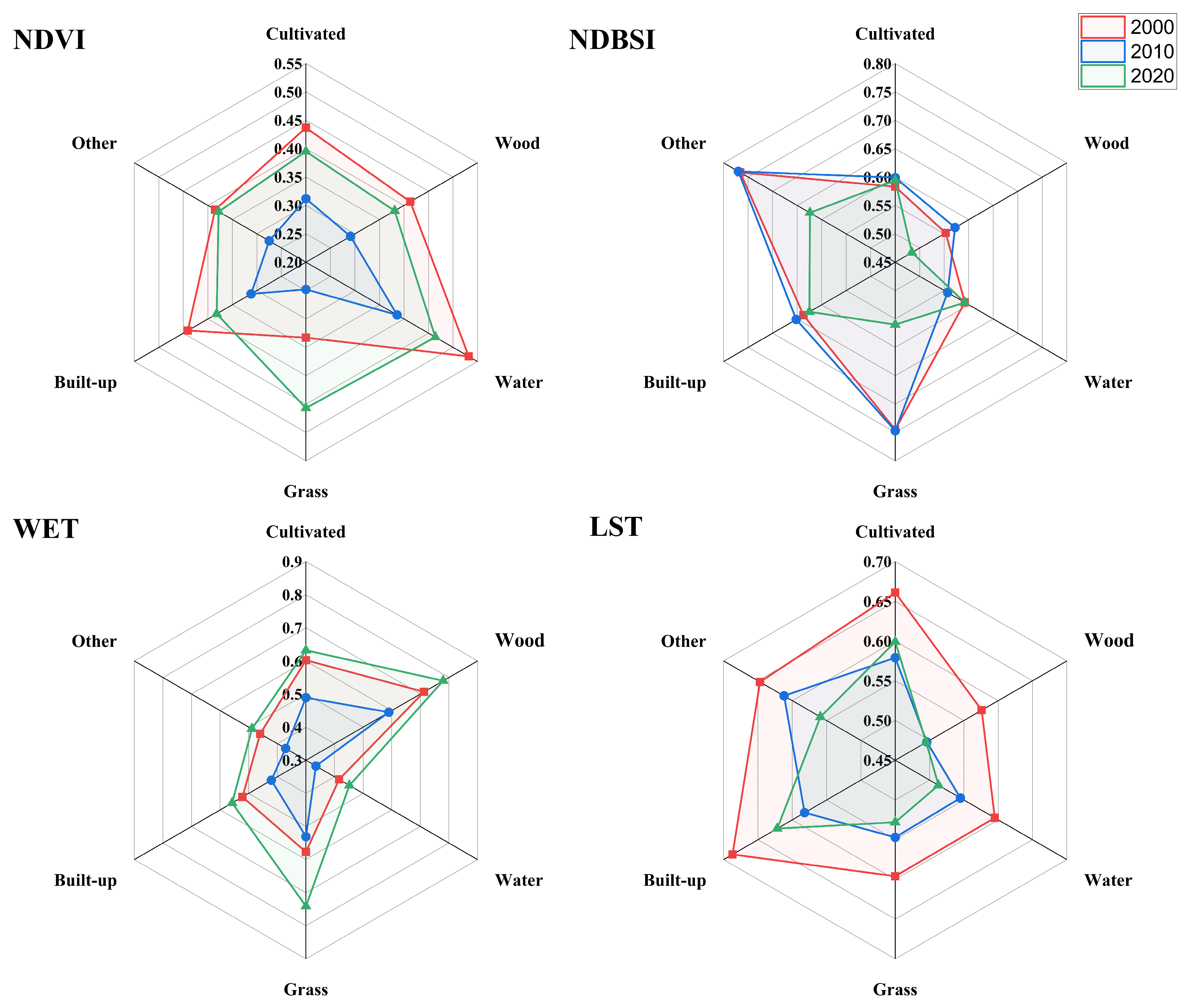
Remote sensing technology, due to its advantages, such as its wide coverage, high resolution, and real-time monitoring, provides important technical support for regional ecological environment assessments [10,11,12,13]. Indicators like the NDVI [14,15], the Normalized Difference Bare Soil Index (NDBSI) [16], Land Surface Temperature (LST) [17], and WET enable long-term ecological monitoring of vegetation changes, temperature fluctuations, and land transformations, offering effective technical solutions for vegetation tracking, climate change evaluation, and urbanization studies [18]. 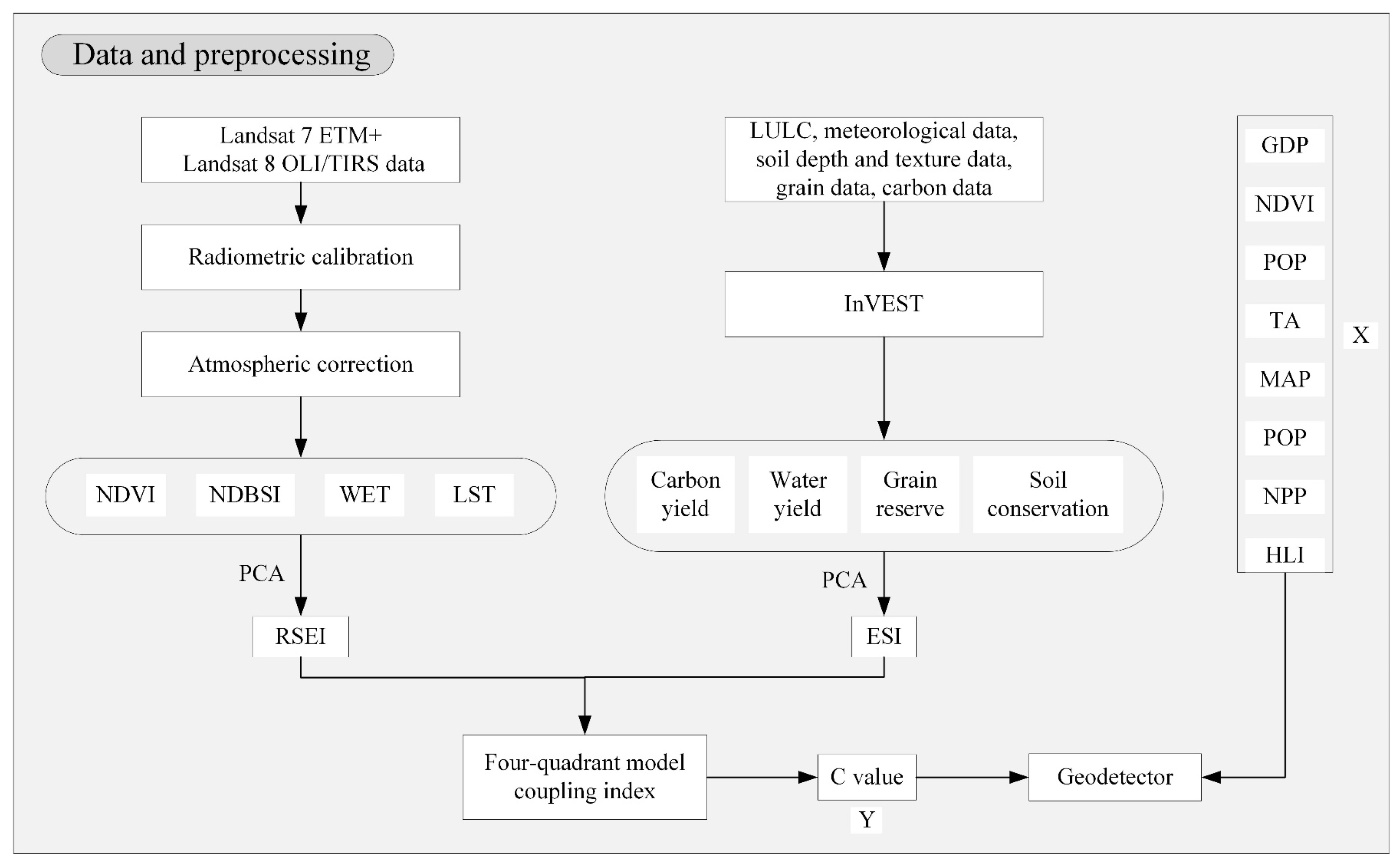However, due to the complexity and diversity of ecosystems, single ecological indices cannot fully capture environmental quality [19]. Therefore, by systematically integrating the four key ecological indicators, namely the NDVI, WET, LST, and NDBSI, and based on principal component analysis (PCA), a comprehensive RSEI was constructed. This index effectively overcomes the limitations of a single ecological indicator and enables a comprehensive quantitative assessment of the regional ecological environment quality [20,21,22]. The RSEI can not only accurately reflect the temporal and spatial evolution characteristics of an ecosystem, but it can also precisely identify the hotspots of ecological degradation. This provides an important spatial decision-making basis for formulating targeted ecological protection and restoration measures [23,24,25].

An ecosystem service assessment quantifies the correlation between ecological functions and human well-being, providing key technical support for the quantitative assessment of ecosystem health and the identification of potential degradation risks [26,27,28,29]. As an important basis for regional sustainable development decisions, the four core indicators, namely carbon storage capacity (reflecting the climate regulation function), water yield (indicating the potential for water resource supply), soil retention capacity (measuring the efficacy of soil erosion prevention and control), and food supply (representing the level of biological productivity), have formed the benchmark framework for ecosystem service evaluations [30,31,32]. However, traditional assessment methods (such as physical measurement methods and market value methods) have obvious limitations: They are unable to comprehensively quantify the multi-dimensional service value of ecosystems, and fail to fully reflect the interactive influence of human activities and ecological processes [33]. The proposed ESI is specifically designed to address these shortcomings. It integrates the biological and physical data provided by methods such as the Integrated Valuation of Ecosystem Services and Tradeoffs (InVEST) model and remote sensing, thereby reducing the reliance on socio-economic indicators and directly capturing often overlooked ecosystem features, such as landscape connectivity and ecological restoration capabilities [33]. Therefore, by using four key ecological indicators, namely carbon storage capacity, water yield, soil retention capacity, and food supply, and based on PCA, the ESI was constructed. This model–data hybrid approach enhances the objectivity of ecosystem assessments by reducing the anthropogenic interference in parameter weighting processes, while preserving the intrinsic relationships between ecosystem structures and functions. The ESI provides a quantifiable spatial decision-making tool for optimizing ecological compensation policies and delineating ecological protection red lines, which is conducive to the coordinated advancement of ecological protection and sustainable development [30,31,32].

Although the RSEI and ESI provide independent assessment frameworks from the perspective of ecological environment quality itself and ecosystem service functions, respectively, they have natural complementarity in terms of representing the co-evolution of the human–environment relationship. 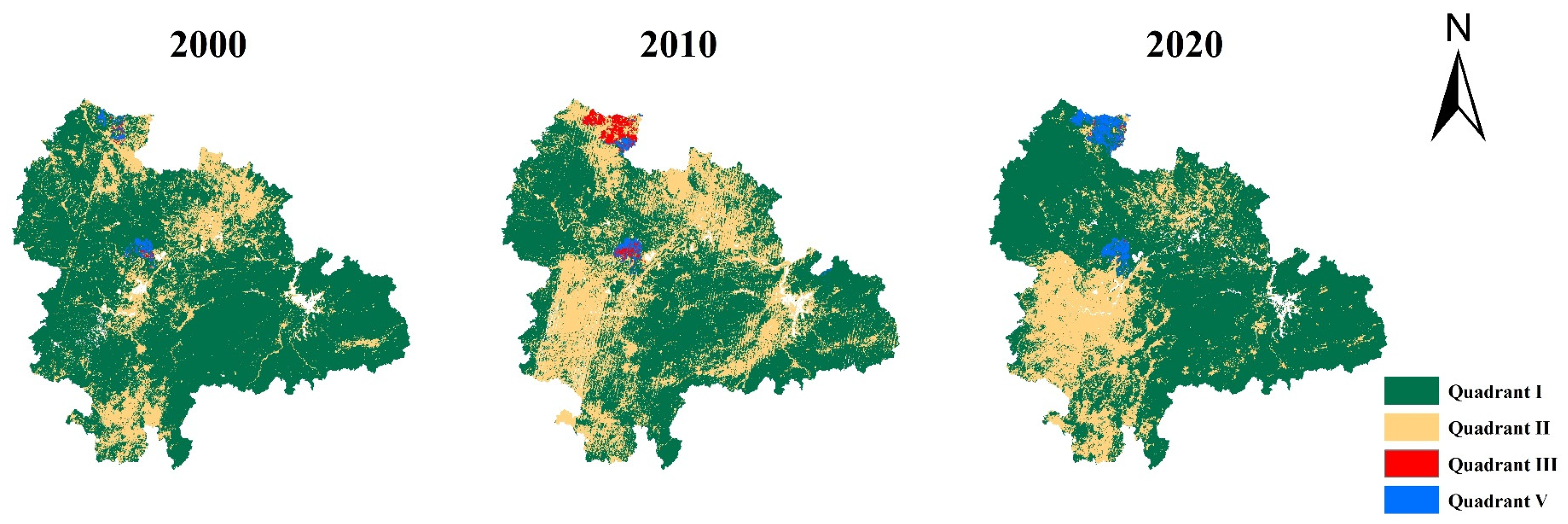By coupling the ecological state monitoring capability of the RSEI with the service value quantification function of the ESI, a ‘state–service’ dual-dimensional evaluation system can be constructed, breaking through the limitations of single perspective assessments [34,35]. To deepen this coupled evaluation framework, this study introduced a four-quadrant spatial zoning model [36,37]. Based on the thresholds of the RSEI and ESI, the study area was divided into four characteristic types of zones: high RSEI–high ESI (high-quality synergy zone), high RSEI–low ESI (potential transformation zone), low RSEI–high ESI (pressure-bearing zone), and low RSEI–low ESI (degradation and restoration zone). To deeply explore the mechanism of the impact of human activities on the ecosystem, this study proposes the use of the coupling coefficient C to quantify the degree of synergy between the RSEI and ESI in regard to different land use types and spatial divisions. This study innovatively introduced the geographical detector method [38], deeply analyzing the spatial differentiation characteristics and driving mechanisms of the coupling coefficient C value between the RSEI and ESI, quantitatively evaluating the independent contribution of each environmental factor to the spatial distribution of the C value, and accurately identifying the key driving factors affecting the “state–service” synergy relationship of the ecosystem. Through the use of factor interaction detection, the collaborative influence mechanism of natural elements and human activities on the C value was revealed, which has significant methodological innovation value [39].

Addressing these research gaps, this study utilizes multi-source remote sensing data to analyze the spatiotemporal changes and driving forces of the ecological benefits in the UAMRYR, establishing scientific foundations for refined territorial spatial governance. The research framework comprises three components: (1) an evaluation of the spatiotemporal variations in land use types, the RSEI, and the ESI within the study area, from 2000 to 2020; (2) the use of a coupled model to quantitatively analyze the collaborative evolution relationship between the RSEI and the ESI from 2000 to 2020, and the use of statistical correlation tests to conduct an objective assessment; and (3) the identification of key drivers influencing the RSEI–ESI coupling dynamics and the analysis of their driving mechanisms and interaction effects.

2. Methods and Materials

2.1. Study Area

The UAMRYR (located at 28°30′–31°50′ N, 111°30′–118°30′ E) is situated in the three provinces of Hubei, Hunan, and Jiangxi, covering an area of 317,400 square kilometers (Figure 1). This region has a mid-subtropical monsoon climate, with an average annual temperature of 16–18 °C and an average annual precipitation of 1200–1600 mm (70% occurring from May to September). The terrain is mainly composed of alluvial plains formed by the Yangtze River and its tributaries (with an altitude of 20–50 m), and the surrounding areas gradually transition to low mountains and hills (100–300 m).

The UAMRYR is a key national ecological function area and also an important economic development region in China. In recent years, rapid urbanization and industrialization have posed severe challenges to the environmental quality and ecosystem service functions in this region. As a typical area sensitive to human–land relations, the ecosystem in this region is facing problems, such as a decline in biodiversity and a weakening of the water conservation capacity. This study selects this region to reveal the coordinated evolution laws of environmental quality and ecosystem service functions during the urbanization process through coupling remote sensing ecological indices and ecosystem service indices, in order to provide a scientific basis for regional sustainable development.

2.2. Data and Preprocessing

(1)

LULC data for the study area was sourced from the Geospatial Data Cloud (https://www.gscloud.cn, accessed on 1 March 2025). Additionally, we employed six LULC categories, namely cropland, forest, water body, grassland, built-up land, and others, to analyze the spatiotemporal changes in land types within the UAMRYR from 2000 to 2020 [40].

(2)

The Geospatial Data Cloud (https://www.gscloud.cn, accessed on 3 March 2025) is an online platform, which was established in 2008 by the Computer Network Information Center of the Chinese Academy of Sciences. Leveraging next-generation information technologies, such as cloud computing and big data, it offers services for searching, acquiring, storing, analyzing, and visualizing geospatial data for researchers.

(3)

The meteorological data was sourced from the National Tibetan Plateau Data Center (data.tpdc.ac.cn). The spatial distribution of precipitation and potential evapotranspiration was determined through the use of interpolation analysis.

(4)

Data on soil depth and texture was obtained from the Harmonized World Soil Database (HWSD) (https://www.fao.org/soils-portal/soil-survey/soil-maps-and-databases/harmonized-world-soil-database-v12/en/, accessed on 5 March 2025).

(5)

GEE (Google Earth Engine) datasets were used. We utilized this platform to process and calculate four remote sensing indices and the RSEI using Landsat 7 ETM+ and Landsat 8 OLI/TIRS data. Landsat 7 ETM+ sensor data has been continuously available since its launch in 1999, while Landsat 8 OLI/TIRS sensor data has been available since its launch on 11 February 2013.

(6)

InVEST is an open-source software toolset for ecosystem service assessments. It offers various models for calculating and analyzing ecosystem service indices. We used this software to compute four ecosystem service indices.

To facilitate the analysis and processing of spatial data, all the information was uniformly converted to the WGS_1984_UTM_Zone_51N coordinate and projection system. The resolution of the remote sensing imagery and land use data used in this study was 30 m.

2.3. Methods

The technical roadmap for this study is presented as follows (Figure 2):

2.3.1. RSEI Indicator Selection

The RSEI comprehensively evaluates ecological quality using four primary ecological indicators: NDVI, NDBSI, LST, and WET [39,40]. These indicators are primarily derived from multispectral remote sensing imagery data. Through a comprehensive analysis of these four indicators, the RSEI can effectively monitor ecological quality at a regional scale [41]. However, the RSEI may have limitations when applied across different regions, as ecological characteristics vary significantly among regions, potentially leading to inconsistent or incomplete ecological assessment results when using the traditional RSEI method in different regions [42,43]. To more intuitively analyze and compare the spatial distribution and dynamic changes in ecological quality within the UAMRYR, the natural ecological environment index is categorized into five levels: poor (0–0.2), fair (0.2–0.4), moderate (0.4–0.6), good (0.6–0.8), and excellent (0.8–1.0).

The calculation formula for the NDVI is as follows [44]:

$$NDVI=(Ban{d}_{nir1}-Ban{d}_r)/(Ban{d}_{nir1}+Ban{d}_r)$$

(1)

In the formula, Band_nir1 and Band_r represent the reflectance of the multispectral image in the first near-infrared band and the red band, respectively.

The NDBSI is obtained by summing up the Soil Index (SI) and the Index-Based Built-up Index (IBI), and the calculation formula is as follows [45]:

$$NDBSI=(SI+BI)$$

(2)

$$SI={\displaystyle \frac{(Ban{d}_{swir1}+Ban{d}_{red})-(Ban{d}_{nir1}+Ban{d}_{blue})}{(Ban{d}_{swir1}+Ban{d}_{red})+(Ban{d}_{nir1}+Ban{d}_{blue})}}$$

(3)

$$\begin{array}{l}IBI={\displaystyle \frac{2\times Ban{d}_{swir1}/(Ban{d}_{swir1}+Ban{d}_{red})-}{2\times Ban{d}_{swir1}/(Ban{d}_{swir1}+Ban{d}_{red})+}}\\ {\displaystyle \frac{(Ban{d}_{nir1}/(Ban{d}_{nir1}+Ban{d}_{red})+Ban{d}_{green}/(Ban{d}_{green}+Ban{d}_{swir1}))}{(Ban{d}_{nir1}/(Ban{d}_{nir1}+Ban{d}_{red})+Ban{d}_{green}/(Ban{d}_{green}+Ban{d}_{swir1}))}}\end{array}$$

(4)

In the formula, Band_red, Band_green, Band_nir1, and Band_swir2 represent the reflectance of the multispectral image in the red, green, first near-infrared, and first shortwave infrared bands, respectively.

The WET calculation formula is as follows [46]:

$$\begin{array}{l}WET=00.1147\times Ban{d}_{red}+0.2489\times Ban{d}_{nir1}+0.2408\times Ban{d}_{blue}\\ +0.3132\times Ban{d}_{green}-0.3122\times Ban{d}_{nir2}-0.5416\times Ban{d}_{swir1}\\ -0.5087\times Ban{d}_{swir2}\end{array}$$

(5)

In the formula, Band_red, Band_blue, Band_green, Band_nir1, Band_nir2, Band_swir1, and Band_swir2 represent the reflectance values of the multispectral image in the red, blue, green, first near-infrared, second near-infrared, first shortwave infrared, and second shortwave infrared bands, respectively.

The LST calculation formula is as follows [47]:

$$LST=T_b/[1+((\lambda T_b)/\rho )\ln \epsilon ]-273$$

(6)

$$T_b=K_2/(K_1/L+1)$$

(7)

$$L=Gain\times DN+basi$$

(8)

Here, λ represents the central wavelength of the 10th band in the Landsat data, which is 10.9 mm; ρ is calculated as 1.4 × 10⁻²λ; K₁ and K₂ are calibration parameters; T_b denotes the brightness temperature, with the unit Kelvin (K); DN stands for the digital number, representing the grayscale value of a pixel in the Landsat data; Gain and bias are the gain and offset values for the frequency band; and L is the radiance value for the red-hot infrared band, with the unit specified as μm in the original text.

2.3.2. ESI Indicator Selection

This study selects four environmental assessment indicators: carbon storage, water yield, grain storage, and soil conservation. The InVEST model is an open-source software model jointly developed by Stanford University, The Nature Conservancy (TNC), and the World Wide Fund for Nature (WWF). It is primarily used to assess the quantity of ecosystem services and present the results in map form, aiding decision makers in better understanding and quantifying the distribution and value of ecosystem services [48,49,50].

(1) Carbon storage is one of the important services provided by ecosystems. The InVEST model quantifies carbon storage by utilizing data on land use or landscape types, combined with biophysical parameters and spatial data, through the use of specific algorithms and production functions. The calculation formula is as follows [51]:

$$Ctotal=Cabove+Cbelow+Csoil+Cdead$$

In the formula, C_total represents the total carbon stock (in tons, t); and C_above, C_below, C_soil, and C_dead denote the carbon stocks in above-ground biomass, below-ground biomass, soil, and dead organic matter, respectively.

(2) Water yield is a key indicator for assessing the water resource conditions in a region, reflecting the amount of water that the region can produce within a certain period. The InVEST model can be used to conduct quantitative analysis of the changes in water yield within the study area. The calculation formula is as follows [51]:

$$Y_x=(1-{\displaystyle \frac{AE{T}_x}{P_x}})\times P_x$$

(9)

In the formula, Y_x represents the water yield of grid cell x; P_x denotes the annual precipitation of grid cell x; and AET_x stands for the annual actual evapotranspiration of grid cell x.

(3) Grain storage is one of the important ecosystem services provided by ecosystems. The grain production value is allocated based on the proportion of the NDVI in regard to cultivated land across different cities or administrative regions. The calculation formula is as follows [35]:

$$P_i={\displaystyle \frac{NDV{I}_i}{NDV{I}_{sum}}}\times P_{sum}$$

(10)

In the formula, P_i represents the grain yield of the ith pixel; NDVI_i is the NDVI value of the ith pixel on cultivated land; NDVI_sum is the sum of NDVI values across the cultivated land in the region; and P_sum is the total grain production in the region.

(4) Soil conservation is a crucial component of ecosystems, which is vital for maintaining land productivity and reducing soil erosion, and the Revised Universal Soil Loss Equation (RUSLE) is used to quantify soil conservation services. The calculation formula is as follows [35]:

$$Q_{se\_p}=R\times K\times L\times S$$

(11)

$$Q_{se\_a}=R\times K\times L\times S\times C$$

(12)

In the formula, C represents the vegetation cover factor; L is the slope length factor; S is the slope steepness factor; K is the soil erodibility factor; and P is the factor for soil and water conservation practices.

2.3.3. PCA

PCA is a statistical method used to transform a set of potentially correlated variables into a set of linearly uncorrelated variables, known as principal components, through the use of orthogonal transformation. This method is commonly employed for dimensionality reduction to simplify the complexity of datasets, while retaining most of the variability present in the original dataset. In this study, PCA is utilized to extract the first principal component (PC₁) for calculating the four constituent factors of the RSEI and the four constituent factors of the ESI [52,53]. These key indicators are used to assess the level of regional sustainable development through an objective, data-driven approach. Additionally, the application of PCA helps balance the weights among different indicators, thereby avoiding bias in the assessment results caused by uneven weight distribution. Prior to conducting PCA calculations, each ecological factor is scaled to the range of [0, 1] for normalization [54]. The calculation formulas are as follows:

$$Y_{ij}={\displaystyle \frac{X_{ij}-\min (X_j)}{\max (X_j)-\min (X_j)}}$$

(13)

In the formula, Y_ij represents the normalized value of indicator j in year i, with the threshold range of [0, 1]; X_j is the actual value of indicator j in year i; and max(X_j) and min(X_j) denote the maximum and minimum values of statistical indicator j throughout the entire study period, respectively.

The calculation formula for the raw data comprising the RSEI indicators is as follows:

$$X=\left[\begin{array}{llll}{x}_{11}& x_{12}& \cdots & x_{1n}\\ x_{21}& x_{22}& \cdots & x_{2n}\\ x_{31}& x_{32}& \cdots & x_{3n}\\ x_{41}& x_{42}& \cdots & x_{4n}\end{array}\right]={[X_{ij}]}_{m\times n}$$

(14)

In the formula, within matrix X, m and n represent the number of indicators for the RSEI and the number of pixels in each indicator’s image, respectively. Each row vector in the matrix represents an individual indicator.

The calculation formula for the raw data comprising the ESI indicators is as follows:

$$X=\left[\begin{array}{llll}{x}_{11}& x_{12}& \cdots & x_{1n}\\ x_{21}& x_{22}& \cdots & x_{2n}\\ x_{31}& x_{32}& \cdots & x_{3n}\\ x_{41}& x_{42}& \cdots & x_{4n}\end{array}\right]={[X_{ij}]}_{p\times q}$$

(15)

In the formula, within matrix X, p and q denote the number of indicators for the ESI and the number of pixels in each indicator’s image, respectively. Each row vector in the matrix represents an individual indicator.

Calculate the eigenvalues λ_i and eigenvectors U_i of the covariance matrix R to form the transformation matrix T by solving the characteristic equation (λ_i − R)U = 0. Subsequently, arrange the λ_i eigenvalues in ascending order, compute the corresponding unit eigenvectors U_i, and construct a matrix U with Ui as the columns. The transposition of matrix U, denoted as U^ᵀ, serves as the desired transformation matrix, T.

The row vectors of the new variables obtained after principal component transformation are referred to as PC₁, PC₂, PC₃, and PC₄. These new variables are assigned to each pixel to reconstruct them into a two-dimensional image, resulting in four principal component images.

The calculation formula for the covariance matrix R is as follows:

$$R={\displaystyle \frac{1}{n-1}}{\displaystyle \sum _{k=1}^n(X_{ki}-{\overline{X}}_i)}(X_{ji}-{\overline{X}}_j)$$

(16)

Finally, the RSEI and the ESI for the study area were calculated using the PCA method. The calculation formulas are as follows:

$$RES{I}_0=f(NDVI,NDBSI,LST,WET)$$

(17)

$$RESI={\displaystyle \frac{RES{I}_0-RES{I}_{\min }}{RES{I}_{\max }-RES{I}_{\min }}}$$

(18)

$$ES{I}_0=F(CS,WC,SR,SE)$$

(19)

$$ESI={\displaystyle \frac{ES{I}_0-ES{I}_{\min }}{ES{I}_{\max }-ES{I}_{\min }}}$$

(20)

In the formula, RSEI₀ and ESI₀ represent the PC₁ obtained from performing PCA of the four normalized indicators. The RSEI is derived by normalizing RSEI₀, and ESI is obtained by normalizing ESI₀.

2.3.4. Four-Quadrant Model

In this study, the four-quadrant model was employed to quantify the coupling relationship between the RSEI and the ESI [55]. With the ESI as the horizontal axis (X) and the RSEI as the vertical axis (Y), a threshold of 0.5 was used to divide the values into high and low categories. The standardization method was used, according to reference [55]. In Figure 3, Four characteristic regions were defined: Quadrant I (RSEI > 0.5–ESI > 0.5) was the dual-optimistic area of ecological quality and services, Quadrant II (RSEI < 0.5–ESI > 0.5) was the area dominated by services but with ecological degradation, Quadrant III (RSEI < 0.5–ESI < 0.5) was the dual-low degraded area, and Quadrant IV (RSEI > 0.5–ESI < 0.5) was the area with potential for ecological restoration. The system revealed the interactive characteristics of the two indicators.

Based on 30 m × 30 m grid units, a spatial distribution map was generated using the raster calculator on the ArcGIS 10.8 platform, and the area proportions of each quadrant were statistically analyzed [35]. This approach enabled the spatial visualization and quantitative assessment of the coupling relationship. By discretizing the continuous indices into typical type areas, this method effectively identified the strengths and weaknesses of the regional ecosystem, providing a scientific basis for differentiated governance.

2.3.5. Coupling Index

The coupling index can be used to evaluate the synergistic relationship between the RSEI and the ESI, aiming to measure the degree of interaction between the two systems [35,55]. This study integrates the RSEI and the ESI, aiming to analyze the ecological benefits and the causes of their changes through the use of the coupling index, while leveraging the ESI’s characteristic of comprehensively reflecting changes in ecological benefits based on the same temporal scale to compensate for the limitation of the RSEI’s evaluation, which is confined to the above-ground components, and to utilize the RSEI’s rapidity and real-time performance based on the spatial scale to offset the ESI’s lag.

This method innovatively integrates the advantages of two indices: On the one hand, it utilizes the characteristics of the ESI’s comprehensive elements and annual statistics to overcome the limitation of the RSEI, which only reflects the changes in surface vegetation coverage; on the other hand, it leverages the 30 m high-resolution remote sensing data and quarterly update capability of the RSEI to overcome the annual data lagging problem of the ESI. Through the coupling index spatiotemporal analysis, the degree of ecological benefit changes can be quantitatively assessed and also the key driving areas can be identified through the use of spatial heterogeneity detection, providing a decision-making basis for ecological management that is both timely and comprehensive. The calculation formula is as follows:

$$C=\sqrt{{\displaystyle \frac{RESI\times ESI}{\frac{1}{2}{(RESI+ESI)}^2}}}$$

In the formula, C represents the coupling index, which is normalized to the range of [0, 1] in this study.

2.3.6. Geodetector Mode

Considering the comprehensive impacts of natural and anthropogenic factors on the coupling index of the RSEI and ESI, as well as the ease of data acquisition, this study selects Gross Domestic Product (GDP), the NDVI, Population Density (POP), the Mean Annual Temperature (TA), MAP, Net Primary Productivity (NPP), and the Human Light Index (HLI) as independent variables, and the coupling index C value of the RSEI and the ESI as the dependent variable for causal relationship identification [56,57,58]. Geodetector is utilized to examine the spatial heterogeneity of individual variables; it is also employed to test the coupling of the spatial distribution between two variables, thereby exploring potential causal relationships between them. The q value in Geodetector assesses the degree of influence exerted by one or multiple factors on the spatial distribution of the study object. The q value ranges between 0 and 1, with a higher value indicating a greater influence [59,60,61]. The calculation formula is as follows:

$$q=1-{\displaystyle \frac{{\displaystyle {\sum }_{k=1}^L{N}_k{\sigma }_k^2}}{N{\sigma }^2}}=1-{\displaystyle \frac{SSW}{SST}}$$

$$SSW={\displaystyle \sum _{k=1}^L{N}_k{\sigma }_k^2}, SST=N{\sigma }^2$$

In the formula, L represents the number of categories of the factor; N_k and N denote the sample sizes of sub-region k and the entire study area, respectively; ${\sigma }_{\kappa }^2$ and σ² represent the variances of sub-region k and the entire study area, respectively; and SSW and SST are the within-group sum of squares and the total sum of squares, respectively.

3. Results

3.1. Changes in LULC from 2000 to 2020

Different LULC types exhibit significant disparities in terms of ecosystem services and functions, leading to varied responses of various LULC types to the RSEI and the ESI. Ecosystems such as forests and wetlands, which possess strong service functions, tend to have relatively high RSEI and ESI values; in contrast, areas with intensive human activities like built-up land, where ecosystem service functions are weaker, typically exhibit lower RSEI and ESI values. Each LULC type, through its unique ecological attributes and functions, exerts varying degrees of influence on the quality of the regional ecological environment and sustainable development.

In Figure 4 and Figure 5, and

Table 1. Different LULC areas from 2000 to 2020. Source: author composition.

Area (104 km2)	2000	2010	2020
Cultivated	14.811	14.827	14.805
Wood	14.5	14.268	14.005
Water	1.649	1.601	1.528
Grass	0.029	0.021	0.008
Built-up	0.706	0.979	1.352
Other	0.005	0.004	0.002

, cultivated land occupies the largest proportion of the region, with areas of 148,110 km² in 2000, 148,270 km² in 2010, and 148,050 km² in 2020, accounting for approximately 47% of the total area; forest land ranks second, with areas of 145,000 km² in 2000, 142,680 km² in 2010, and 140,050 km² in 2020, comprising about 46% of the total area. A synthesis of the data in Figure 4 and Table 1 reveals that the LULC dynamics in the study area from 2000 to 2020 were primarily characterized by the building up of natural land driven by urban expansion, resulting in a substantial increase in built-up land (by approximately 5460 km² in total), with its east–west sprawl directly leading to a continuous decline in the proportions of grass land, water bodies, and other land (grassland decreased by approximately 210 km², water bodies by about 1210 km², and other land by roughly 3 km²).

3.2. RSEI Analysis Results

3.2.1. Changes in RSEI Indicators

As observed from the data in Figure 6 and Figure 7, the NDVI, NDBSI, WET, and LST indices are closely related to the composition types of the LULC. The study area exhibits a prominent characteristic of a “synergy between intensive development and ecological conservation.” Within the NDVI index, significant vegetation restoration is evident in regard to cultivated land and forest land. The NDVI values for both cultivated land (0.632) and forest land (0.78) in 2020 surpassed historical levels, while the NDVI for grassland surged from 0.577 in 2000 to 0.741 in 2020. For the NDBSI index, the NDBSI value for built-up land peaked at 0.652 in 2010, before declining to 0.625 in 2020. Meanwhile, the NDBSI for grassland plummeted from 0.745 to 0.56. Regarding the WET index, while the WET value for water bodies partially recovered from 0.386 in 2010 to 0.464 in 2020, the WET for grassland increased from 0.333 to 0.457. Within the LST index, cultivated land and built-up land exhibit fluctuating adjustments. The LST of cultivated land decreased from 0.661 in 2000 to 0.579 in 2010, before rebounding to 0.599 in 2020. Similarly, the LST of built-up land dropped from 0.687 in 2000 to 0.582 in 2010 and then rebounded to 0.622 in 2020. In contrast, the LST values for forest land, water bodies, and grassland continued to decline.

3.2.2. Changes in RSEI

As shown in

Table 2. Changes in RSEI for each type of LULC in the study area from 2000 to 2020. Source: author composition.

Year	Cultivated	Woodland	Water	Grass	Built-Up	Other	RESI
2000	0.788	0.799	0.782	0.805	0.776	0.767	0.808
2010	0.821	0.800	0.824	0.820	0.838	0.811	0.803
2020	0.818	0.796	0.810	0.806	0.804	0.849	0.802

and Figure 8, the regional urban agglomeration of the RSEI in the UAMRYR area exhibited a spatially differentiated evolution pattern from 2000 to 2020: The regional comprehensive RSEI decreased from 0.808 in 2000 to 0.802 in 2020, with a brief fluctuation (0.803) in 2010. In terms of land use types, the RSEI of cultivated land continuously increased from 0.788 in 2000 to 0.818 in 2020; the RSEI of built-up land significantly rose from 0.776 in 2000 to 0.804 in 2020; whereas the RSEI of forest land, water bodies, and grassland showed a trend of an “initial increase followed by decrease.”

According to the PCA results detailed in

Table 3. Principal component eigenvalues and contribution rates of RSEI indicators from 2000 to 2020. Source: author composition.

Year	NDVI	NDBSI	WET	LST	Contribution Rate (%)
2000	0.013	0.007	0.005	0.002	75.63
2010	0.010	0.007	0.006	0.003	63.45
2020	0.018	0.013	0.005	0.002	81.23

, the principal component eigenvalues and contribution rates of the RSEI indicators for the UAMRYR from 2000 to 2020 exhibited significant spatiotemporal differentiation. The eigenvalue of the NDVI fluctuated and increased from 0.013 in 2000 to 0.018 in 2020, which is consistent with the findings in [62]. The eigenvalue of the WET remained stable at 0.005 from 2000 to 2020, reflecting the fundamental supporting role of hydrological conditions on the stability of ecosystems [63]. The eigenvalue of the NDBSI increased from 0.007 in 2000 to 0.013 in 2020. The eigenvalue of the LST peaked at 0.003 in 2010, confirming the negative inhibitory effect of built-up land expansion and the intensification of the heat island effect on the RSEI [64]. In terms of contribution rates, the contribution rate of PC₁ was 75.63%, 63.45%, and 81.23% in 2000, 2010, and 2020, respectively, all exceeding 60%, which meets the validity criteria for PCA₁ as an explanatory variable in principal component analysis [65]. Among them, the eigenvalue of the NDVI accounted for the highest proportion of PC₁ (reaching 0.018 in 2020), further verifying its status as the dominant driving factor of the RSEI.

3.3. ESI Analysis Results

Changes in ESI Indicators

From Figure 9 and Figure 10, it can be seen that the normalized results of carbon storage, water yield, grain storage, and water and soil conservation services in the study area are closely related to the temporal and spatial evolution of different LULC types. Spatially, the spatial distribution differences in the ecosystem service supply in different periods are not significant, but there are significant differences among different types of ecosystem service supply. Among them, water supply shows a spatial pattern of “low in the northwest and high in the southeast”, which is related to the annual average precipitation and land use types in the UAMRYR; carbon supply and soil supply show a spatial pattern of “high in the northwest, low in the central part, and high in the southeast”, which is related to the annual average temperature and CO² emissions, and the distribution is not certain; the high value of grain supply is distributed in the areas along the lakes, such as Xiangyang City, Jingmen City, and Changde City, where the climate conditions are suitable for vegetation growth and human activities are low.

As indicated in

Table 4. ESI changes for each LULC type in the study area from 2000 to 2020. Source: author composition.

Year	Cultivated	Woodland	Water	Grass	Built-Up	Other	ESI
2000	0.774	0.857	0.875	0.890	0.852	0.811	0.745
2010	0.776	0.883	0.832	0.859	0.847	0.795	0.747
2020	0.775	0.883	0.858	0.848	0.883	0.893	0.746

, during the spatiotemporal evolution of the ESI in the UAMRYR from 2000 to 2020, the change characteristics of forest land and built-up land were particularly notable. The ESI of forest land increased from 0.857 in 2000 to 0.883 in 2010 and remained at this level until 2020, indicating a continuous enhancement of forest ecological functions. The ESI of built-up land rose from 0.852 in 2000 to 0.883 in 2020. The ESI of cultivated land remained stable within the range of 0.774–0.775 from 2000 to 2020, confirming the resilience characteristics of grain production and soil carbon sequestration. As can be seen from Figure 9 and Figure 11, the distribution pattern of high and low values of the ESI in the study area is consistent with that of the four categories of ecosystem service indicators, indicating that the ESI can effectively quantify the supply capacity of regional ecosystem services. It is noteworthy that the ESI of other land uses jumped from 0.811 in 2000 to 0.893 in 2020, which may be attributed to the implementation of ecological restoration projects on unused land.

Combining Figure 10 and Table 4, the ESI of each land use type in the study area showed differentiated evolution characteristics from 2000 to 2020. Overall, the comprehensive ESI of the study area remained relatively stable, increasing from 0.745 in 2000 to 0.746 in 2020. Specifically for each land use type: the ESI of forest land was the most prominent, significantly increasing from 0.857 to 0.883, with an increase of 3.0%, confirming the continuous improvement of the forest ecosystem; the ESI of water bodies showed fluctuating changes, dropping to 0.832 in 2010 and then rising to 0.858 in 2020, but still not returning to the 2000 level (0.875); the ESI of grassland showed a continuous downward trend, decreasing from 0.890 to 0.848, with a decline of 4.7%, reflecting the significant pressure on the grassland ecosystem. Notably, the ESI of construction land increased against the trend, from 0.852 to 0.883, possibly related to ecological restoration measures, such as urban greening construction; the ESI of other land types increased significantly (0.811→0.893), with an increase of 10.1%. The differentiated evolution of each type of ESI indicates that the regional ecosystem has undergone structural adjustments. Among them, the ecological function of forest land has continued to strengthen, while grassland and water bodies face different degrees of degradation risks.

Combining the data from

Table 5. Principal component eigenvalues and contribution rates of ESI indicators from 2000 to 2020. Source: author composition.

Year	Carbon Yield	Water Yield	Grain Reserve	Soil Conservation	Contribution Rate (%)
2000	0.04	0.015	0.002	0.001	76.92
2010	0.12	0.01	0.003	0.002	91.3
2020	0.115	0.012	0.003	0.002	89.29

and Figure 8, the 20-year study on the ESI of the UAMRYR, based on PCA, reveals that the four indicators of carbon storage, water yield, grain storage, and soil conservation services have a significant positive driving effect on the ESI. The contribution rate of PC₁ exceeds 70%, validating the scientificity of using PC₁ to represent the ESI. Among these indicators, the eigenvalue of carbon storage increased from 0.04 in 2000 to 0.115 in 2020, becoming the core driving factor of ecological service capacity. The eigenvalue of water yield is generally low, ranging from 0.012 to 0.015. It shows a typical characteristic where urban expansion leads to a higher water yield but a lower ESI, while forested areas exhibit a lower water yield but a higher ESI. The spatial differentiation characteristics are as follows: in the cultivated land-concentrated areas of urban cores and transportation radiation belts, the ESI continues to decline, ranging from 0.852 to 0.883, indicating a significant trend of ecological degradation. High-value areas, with an ESI ranging from 0.857 to 0.883, are stably distributed in the northern mountainous forested areas and the southeastern ecological barrier zones, highlighting the prominent role of forest cover in enhancing ecological services.

3.4. Coupling Relationship Between RSEI and ESI

Figure 3, Figure 12 and

Table 6. The area of each quadrant in the study area from 2000 to 2020. Source: author composition.

Year	Quadrant I	Quadrant II	Quadrant III	Quadrant IV
2000	25.17	6.32	0.04	0.17
2010	19.69	11.42	0.39	0.21
2020	23.34	7.81	0.02	0.52

illustrate that the evolution of land use and ecological coordination in the UAMRYR region exhibits significant spatial differentiation. From a spatial pattern perspective, over the 20-year period, Quadrant I (distributed in areas such as the Huangpi District of Wuhan City and the Xiaonan District of Xiaogan City) was predominantly characterized by forest land and cultivated land. Its area exhibited a fluctuating trend of an initial decrease followed by an increase, with an overall reduction of 18,300 km². Quadrant II (located in agricultural areas, such as Tuanfeng County in Huanggang City) experienced an initial increase followed by a decrease in area, but still achieved an overall net increase of 14,900 km². Quadrant III (distributed in urban areas, such as the Honggutan District of Nanchang City and the Xunyang District of Jiujiang City) was primarily dominated by built-up land. Its area fluctuated significantly, with an overall reduction of 200 km². This can be attributed to the high-intensity adjustments in land use resulting from the rapid urbanization of the core urban agglomeration. Quadrant IV (distributed in scattered forested areas, such as the Yiling District of Yichang City) was predominantly characterized by forest land, with a continuous increase in area of 3500 km².

The quadrant model, by integrating the RSEI and the ESI, systematically analyzes the collaborative evolution pattern of regional ecological environmental quality and service capabilities. From 2000 to 2020, the spatial differentiation characteristics of ecological quality and service capabilities in the study area indicate the following: The contradiction between urbanization and ecological conservation is particularly prominent in Quadrants I and III. In contrast, Quadrants II and IV have achieved localized optimizations of ecological-production functions through the intensive utilization of cultivated land and forest restoration, respectively [66].

3.5. Coupling Level Between RSEI and ESI

Figure 13 illustrates that the spatial heterogeneity of the UAMRYR coupling index from 2000 to 2020 was significant, forming clusters of high and low values. The low-value areas were primarily concentrated in regard to the construction land of core urban districts, such as Wuhan, Changsha, and Nanchang. Influenced by high-intensity urbanization, these areas exhibited a combination of a low RSEI and a low ESI, with the normalized coupling index showing a continuous downward trend. The high-value areas were mainly distributed in Wuling Mountains and Poyang Lake, characterized by a high level of forest and wetland coverage, minimal human interference, high clustering of the RSEI and the ESI, and a steady increase in the coupling index over time. The transitional areas were concentrated in agricultural regions, such as the Jianghan Plain and Dongting Lake Plain, with the LULC predominantly consisting of cultivated land. In the ecologically fragile zones of the mining areas in western Hubei and western Hunan, due to the alternating effects of resource exploitation and ecological governance, the surface vegetation coverage fluctuated, and the coupling index exhibited a “decline–rise–decline” trend.

Table 7. Changes in the coupling index for each LULC type and each quadrant in the study area from 2000 to 2020. Source: author composition.

LULC	2000	2010	2020
Cultivated	0.688	0.685	0.690
Woodland	0.694	0.696	0.696
Water	0.691	0.687	0.692
Grass	0.699	0.696	0.695
Built-up	0.693	0.687	0.692
Other	0.683	0.689	0.699
Quadrant I	0.693	0.692	0.694
Quadrant II	0.693	0.693	0.692
Quadrant III	0.691	0.693	0.691
Quadrant IV	0.687	0.687	0.682

shows that the coupling indices of various land use types and quadrants exhibit differentiated evolutionary characteristics. From the perspective of land use types, the C value of grassland continues to decline (0.699→0.695); the C value of other land uses significantly increases (0.683→0.699); cultivated land, forest land, water bodies, and built-up land show slight fluctuations, but remain generally stable. From the perspective of the quadrant spatial pattern, the C value of Quadrant I slightly increases (0.693→0.694), confirming its dominant position; the C value of Quadrant IV continues to decline (0.687→0.682), suggesting that there is still local ecological pressure during the forest restoration process; the C values of Quadrants II and III show fluctuating adjustments. To explore the coupling degree between the RSEI and the ESI in regard to various synergistic relationships, we calculated the coupling indices of each quadrant in the study area from 2000 to 2020. The average normalized coupling indices of each quadrant in the study area from 2000 to 2020 are as follows: Quadrant I (0.6930) > Quadrant II (0.6927) > Quadrant III (0.6917) > Quadrant IV (0.6853).

3.6. GTWR Analysis Results

In this study, a quantitative analysis of the driving factors and their interactions was conducted using the “factor detection” and “interaction detection” functions of the Geodetector tool. The study aimed to explore the dominant factors contributing to the spatial differentiation of the C value in the UAMRYR. Additionally, the characteristics of the interactions among various driving factors were investigated. Ultimately, the factor detection result map (Figure 14) and interaction detection result map (Figure 15) of the spatial differentiation were obtained.

3.6.1. Analysis of Dominant Factors

Figure 14 indicates that the contribution rates of the driving factors exhibited significant spatial–temporal differentiation from 2000 to 2020. The contribution rate of the GDP peaked at 0.24782 in 2010, marking a 64% increase from 2000, before sharply declining to 0.10338 in 2020. The NDVI showed a continuous upward trend (0.51861→0.5605). The contribution rate of the NPP surged to 0.40394 by 2010, but then dropped to 0.21801 in 2020. The POP demonstrated a fluctuating pattern of “rise and fall” (0.20427→0.23919→0.10039), reflecting the phased characteristics of urbanization. The contribution rate of the TA doubled (0.1379→0.27579). The MAP decreased by 17% (0.46609→0.38499). The NLI exhibited a gradual decline (0.24649→0.20481).

3.6.2. Interaction Identification

Figure 15 illustrates that the spatial differentiation pattern of C in the UAMRYR region from 2000 to 2020 was predominantly driven by the synergistic effects of multi-factor interactions, with the intensity of these interactions significantly increasing over time. The coupling effects between economic and natural factors are evident: The interaction intensity between GDP and MAP rose from 0.5186 in 2000 to 0.9358 in 2020; the interaction intensity between the NLI and TA surged from 0.4433 to 0.7190, which in addition to the urban heat island effect with climate warming, have significantly amplified regional disparities and ecological patterns. The interaction characteristics between ecological and social factors reveal that the interaction intensity between the POP and NPP reached 0.8438 in 2010; the interaction intensity between the NDVI and TA approached the threshold of 1 in 2020, highlighting the dynamic pressure exerted by human activities on the ecological carrying capacity and the extreme stress imposed by economic development on ecological sensitivity.

4. Discussion

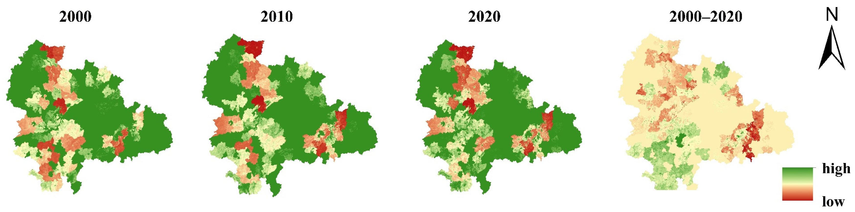
4.1. RSEI Variation Analysis

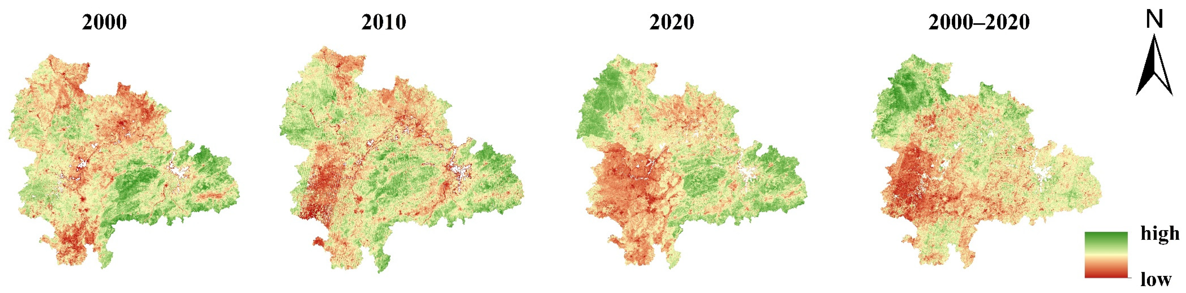
A comprehensive analysis of Figure 3 and Figure 6 reveals that the evolution of the LULC in relation to the RSEI values in the UAMRYR region from 2000 to 2020 exhibited significant synergistic characteristics. Areas with high RSEI values were concentrated in the wetlands of Dongting Lake, the Mufu Mountain forest belt, and the water body protection zones along the mainstream of the Yangtze River. The increase in forest land and water body coverage in these areas underscored the supportive role of the natural ecological foundation in maintaining ecosystem quality. Areas with low RSEI values were primarily located in the Wuhan Metropolitan Area, where the expansion of built-up land significantly overlapped. The changes in cultivated land demonstrated a dual regulatory pattern: the intensification of farmland in the Jianghan Plain through water-saving irrigation slightly increased the RSEI, while the fragmentation or abandonment of cultivated land in suburban areas led to a decline in the RSEI. The spatial expansion of the region followed a pattern of “expanding eastward into the Jianghan Plain and westward into the hilly and mountainous areas.” The spread of built-up land in the Wuhan and Changsha–Zhuzhou–Xiangtan urban agglomerations encroached upon the ecological spaces of traditional agricultural areas in the central region.

Ecological restoration projects have achieved remarkable results, yet significant regional disparities exist: The project of converting farmland back to lakes in the Dongting Lake area and the project of converting farmland to forests in the mountainous regions of western Hubei have, respectively, enhanced the RSEI values by restoring water bodies and forest lands. The Wuhan Green Core Project has focused on restoring fragmented urban habitats through ecological corridors. However, the resurgence of land reclamation around Poyang Lake has led to a decrease in grassland areas and a decline in the RSEI values, indicating that ecological restoration efforts require long-term policy guarantees.

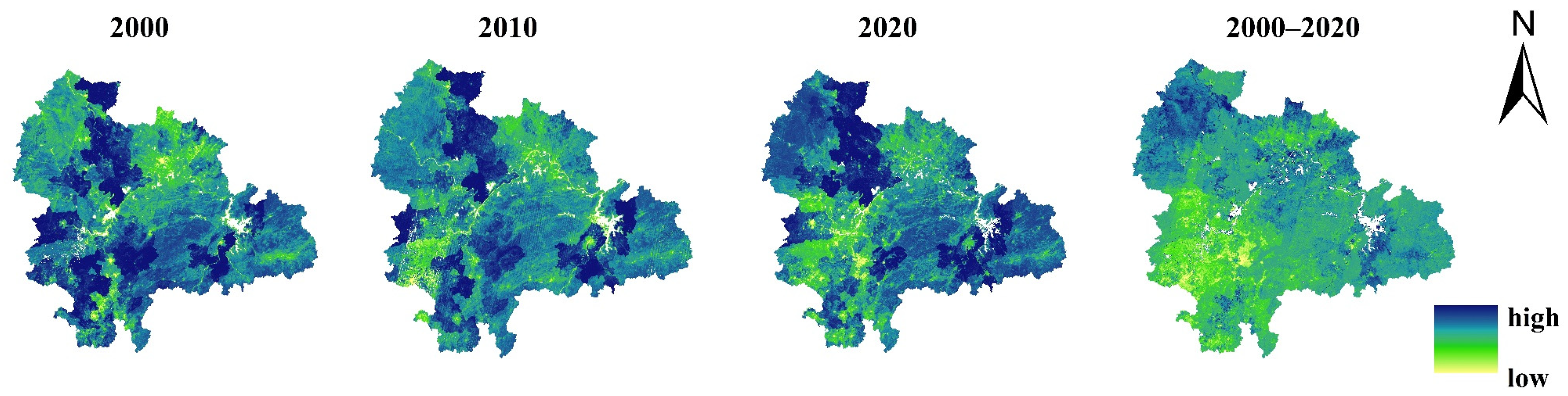
4.2. ESI Variation Analysis

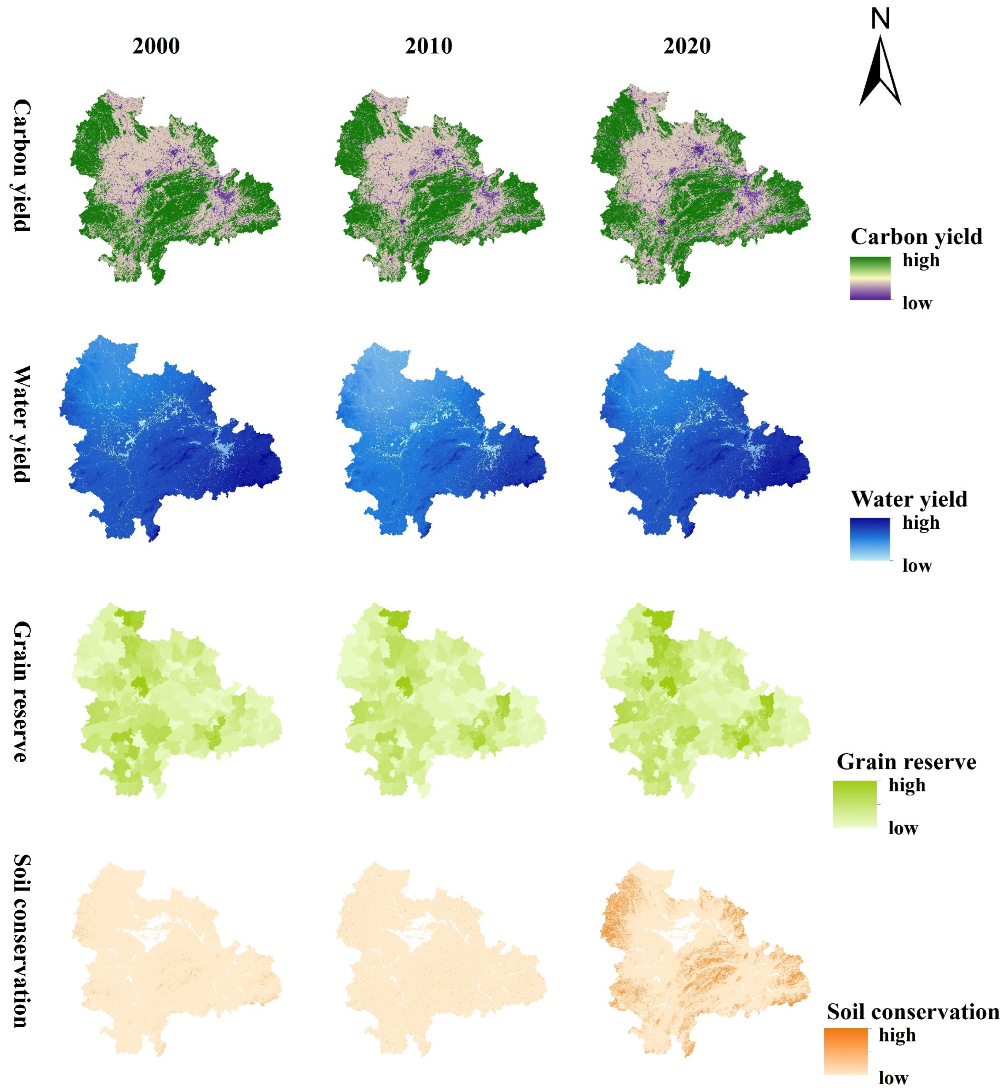
Figure 9 and Figure 11 illustrate that there is a pronounced gradient in carbon sequestration, soil conservation, and water yield services, following the order of forestland > cropland > built-up land. In contrast, the trend for grain production services exhibits an inverse pattern, namely built-up land > cropland > forestland. These findings are consistent with the ecological functional characteristics of land use: Forestland, due to its high vegetation cover and deep soil structure, plays a dominant role in carbon sequestration and soil and water conservation functions. Although cropland is more efficient in regard to grain production, its ecological regulatory capacity is weaker than that of forestland. Built-up land, with its increased surface impermeability, significantly enhances water yield service capabilities, but contributes less to grain production.

The PCA further unveils the trade-off relationships among regulatory services across various land use types, such as the heterogeneity in hydrological regulation between water bodies and grasslands, as well as the intensifying impact of built-up land expansion on water availability. PCA is used to construct a comprehensive ESI by extracting principal components from multiple indicators, thereby circumventing subjective weight assignments, and objectively reflecting the spatial differentiation characteristics of ecosystem services within the study area, thus offering robust data support for ecological assessments.

4.3. Coupling Relationship and Coupling Level Analysis Between RSEI and ESI

During the process of ecological and environmental changes in the UAMRYR region, the C value between the RSEI and the ESI exhibits distinct spatial–temporal differentiation characteristics, effectively reflecting the synergistic relationship between the RSEI and the ESI amidst changes in ecological and environmental quality. An analysis combined with LULC changes reveals that the process of built-up land encroaching upon the ecological space of cropland often leads to a rapid decline in the RSEI, while the ESI tends to decrease more slowly due to its inherent lag effect. In areas significantly affected by human engineering activities, such as regions undergoing rapid urban expansion and industrial development, both the RSEI and the ESI tend to decline concurrently. Issues such as the destruction of natural vegetation and soil pollution during the urbanization process have led to a dual impairment of both ecological and environmental quality and ecosystem service functions. Consequently, the NDVI in these areas has decreased significantly, reflecting the dual pressures exerted by human activities on the ecological environment.

It is recommended to establish a synergistic monitoring framework for the RSEI–ESI, prioritizing the construction of ecological corridors in areas undergoing built-up land expansion to interrupt the cascading effect of “RSEI decline–ESI lagging deterioration,” and to implement conservation tillage practices in major agricultural production areas to mitigate the “hidden depletion” of the ESI, thereby supporting the optimization of territorial spatial resilience.

4.4. Spatial Autocorrelation and Driver Analysis

The spatial differentiation pattern in the UAMRYR region is predominantly driven by the dynamic intensification of the synergistic effects among multiple interacting factors. The coupling effects between economic and natural factors unveil the profound contradictions inherent in regional development: The interaction intensity between GDP and MAP has surged dramatically, indicating an intensified reliance of economic growth on climatic resources, which may amplify the potential risks associated with uneven regional water resource distribution. The interaction intensity between the NLI and TA has also skyrocketed, suggesting that the combined effects of urban heat island phenomena and global warming may reshape local microclimates, exacerbating thermal stress on ecosystems. The interactive characteristics between ecological and social factors further underscore the extreme pressures exerted by human activities on ecosystems: The interaction intensity between the POP and NPP was notably high in 2010, reflecting the dynamic compression of the ecological carrying capacity due to population aggregation amidst rapid urbanization. In 2020, the interaction intensity between the NDVI and TA approached 1, serving as a warning that the intensity of economic development has moved toward the critical threshold in terms of ecologically sensitive areas, potentially triggering irreversible ecological degradation. The spatiotemporal evolution of these interactive effects suggests that the maintenance of regional ecological security patterns necessitates transcending the limitations of single-factor regulation, with a primary focus on the dynamic feedback mechanisms subject to the synergistic effects of multiple factors.

The interaction analysis reveals that the nonlinear synergistic effects between economic and natural factors significantly exacerbate spatial heterogeneity. The coupling effects between economic growth and climatic resources have notably amplified regional disparities over time, emerging as the core driving force behind the differentiation of ecological patterns. Meanwhile, the combined effects of urban heat island phenomena and global warming have accelerated the restructuring of ecological patterns in sensitive areas. Simultaneously, the interactive pressures between human activities and the ecological carrying capacity are particularly pronounced in regions undergoing high-intensity development, highlighting the profound disruptions caused by socioeconomic factors to the stability of ecosystems.

5. Conclusions

Based on multi-source remote sensing data, this study has constructed a comprehensive evaluation system for the RSEI and the ESI. By employing the four-quadrant model and the coupling degree model, it has unveiled the spatiotemporal evolution patterns of the ecological environment in the UAMRYR region. Furthermore, it has combined the Geodetector model to analyze the coupling between the RSEI and the ESI, as well as the driving forces and interactions of key influencing factors. This provides an analytical framework for evaluating ecological benefits. The main research conclusions are as follows:

(1)

During the period from 2000 to 2020, the ecological regions within the UAMRYR exhibited dynamic transformation characteristics. The area in the first quadrant diminished by 13,800 km², whereas the areas in the second and fourth quadrants expanded by 14,900 km² and 3500 km², respectively, while the third quadrant remained almost unchanged. It is suggested that the third quadrant should be prioritized as the key area for ecological restoration. Through vegetation restoration projects, the ecological resilience of this area can be enhanced.

(2)

During the period from 2000 to 2020, the RSEI and the ESI in the UAMRYR region exhibited contrasting evolutionary patterns: The RSEI decreased by 0.006, while the ESI exhibited a marginal increase of 0.001. The fluctuations in the RSEI and ESI indicators may reflect the steady-state characteristics of the system, rather than significant ecological changes.

(3)

From 2000 to 2020, the average ranking of the driving factors of ecological changes was as follows: Normalized Difference Vegetation Index > Annual Rainfall > Net Primary Productivity> Nighttime Light Index > Annual Mean Temperature > Population Density > Gross Domestic Product. The NDVI and Annual Rainfall were the dominant factors driving ecological evolution, while economic driving factors, such as GDP, had relatively weaker impacts, indicating the notable effectiveness of ecological priority policies.

This study proposes a three-pillar framework for precision-based ecological restoration: (1) a quadrant-based diagnosis for systematic degradation assessments, (2) Geodetector-driven analysis to quantify driving factors, and (3) RSEI–ESI coupled interventions for targeted restoration. This integrated approach enables spatially explicit, mechanism-informed ecological governance, while maintaining scientific rigor across different scales.

6. Limitations and Future Scope

This study employed the Geodetector model to analyze the spatial heterogeneity impact of natural and socio-economic factors on the coupling relationship between the RSEI and the ESI. By breaking through the linear assumption limitations of traditional regression models, it revealed the cascading driving mechanism of multi-factor interactions, providing a spatially explicit diagnostic tool for identifying the “threshold mutation” risks in ecologically sensitive areas. However, this study has the following limitations: The type of analysis, which is based on medium-resolution remote sensing data, means that it is difficult to capture the responses of micro-ecological processes, which may weaken the representation of the spatial heterogeneity of local ecological feedback. The spatial refinement representation of social driving factors is still insufficient, which may underestimate the potential impact of human factors on ecological regulation. Although the 20-year research period can reflect the recent ecological evolution characteristics, it is not sufficient to capture longer-term climate change trends.

Future research can introduce a multi-source heterogeneous technology integration scheme, for instance, using unmanned aerial vehicle (UAV)-mounted hyperspectral imaging to achieve sub-meter level ecological parameter inversion, combining LiDAR point cloud data to extract three-dimensional vegetation structural features, obtaining real-time environmental gradient data through an Internet of Things sensor network, and integrating multi-temporal remote sensing data and socio-economic big data using deep learning frameworks, thereby constructing an integrated ‘air–ground–network’ monitoring system. This technological combination not only enhances the spatiotemporal continuity of ecological process simulation through multimodal data fusion, but also enables the intelligent completion of missing data areas through the use of algorithms, such as Generative Adversarial Networks (GAN), providing more precise scale support for revealing the patterns of ecological threshold mutations.

References

1. Saik, P.; Koshkalda, I.; Bezuhla, L.; Stoiko, N.; Riasnianska, A. Achieving land degradation neutrality: Land-use planning and ecosystem approach. Front. Environ. Sci. 2024, 12, 1446056. [Google Scholar] [CrossRef]
2. Elo, M.; Kareksela, S.; Ovaskainen, O.; Abrego, N.; Niku, J.; Taskinen, S.; Aapala, K.; Kotiaho, J.S. Restoration of forestry-drained boreal peatland ecosystems can effectively stop and reverse ecosystem degradation. Commun. Earth Environ. 2024, 5, 680. [Google Scholar] [CrossRef]
3. Ding, M.Y.; Shen, Z.Y.; Balezentis, T.; Chen, X.L. Climate change and marginal abatement cost: Policy insights on international treaty. Energy 2025, 321, 135515. [Google Scholar] [CrossRef]
4. Öztürk, S.T.; Toprak, Z.F. The success of the Kyoto Protocol in reducing carbon emissions in the EU. Int. J. Glob. Warm. 2025, 36, 53–66. [Google Scholar] [CrossRef]
5. Salamat, M.R. Ethics of sustainable development: The moral imperative for the effective implementation of the 2030 Agenda for Sustainable Development. Nat. Resour. Forum. 2016, 40, 3–5. [Google Scholar] [CrossRef]
6. Shulla, K.; Leal, W.; Lardjane, S.; Sommer, J.H.; Borgemeister, C. Sustainable development education in the context of the 2030 Agenda for sustainable development. Int. J. Sustain. Dev. World Ecol. 2020, 27, 458–468. [Google Scholar] [CrossRef]
7. Guo, S.J.; Luan, Z.Q.; Liang, W. Does urban agglomeration aggravate regional haze pollution? Empirical evidence from urban agglomerations in the middle reaches of the Yangtze River in China. Environ. Sci. Pollut. Res. 2023, 30, 54666–54681. [Google Scholar] [CrossRef]
8. Wang, L.; Yang, W.Y.; Yuan, Y.Y.; Liu, C.L. Interurban Consumption Flows of Urban Agglomeration in the Middle Reaches of the Yangtze River: A Network Approach. Sustainability 2019, 11, 268. [Google Scholar] [CrossRef]
9. Buchadas, A.; Moreira, F.; McCracken, D.; Santos, J.L.; Lomba, A. Assessing the potential delivery of ecosystem services by farmlands undercontrasting management intensities. Ecol. Soc. 2022, 27, 5. [Google Scholar] [CrossRef]
10. Gong, X.; Li, T.Q.; Wang, R.; Hu, S.; Yuan, S. Beyond the Remote Sensing Ecological Index: A Comprehensive Ecological Quality Evaluation Using a Deep-Learning-Based Remote Sensing Ecological Index. Remote Sens. 2025, 17, 558. [Google Scholar] [CrossRef]
11. Qiu, Y.J.; Xue, J.F.; Zhang, G.; Hao, X.Y.; Lei, T.; Jiang, P. RS-FeatFuseNet: An Integrated Remote Sensing Object Detection Model with Enhanced Feature Extraction. Remote Sens. 2025, 17, 61. [Google Scholar] [CrossRef]
12. Luiselli, L.; Pacini, N. Remote Sensing That Makes Sense in Ecological Research-From Pixels to Conservation. Afr. J. Ecol. 2025, 63, e70002. [Google Scholar] [CrossRef]
13. Van Cleemput, E.; Adler, P.B.; Suding, K.N.; Rebelo, A.J.; Poulter, B.; Dee, L.E. Scaling-up ecological understanding with remote sensing and causal inference. Trends Ecol. Evol. 2025, 40, 122–135. [Google Scholar] [CrossRef] [PubMed]
14. Ke, H.C.; Liang, L.; Tian, M.H.; Wang, M.L.; Yuan, C.H.; Gao, Y.Y. Assessing vegetation dynamics and influencing factors in Northwest China’s Arid Regions: A spatiotemporal analysis using NDVI (2000–2020). Acta Geophys. 2025, 73, 3405–3424. [Google Scholar] [CrossRef]
15. Li, A.; Jiang, M.H.; Chu, D.; Guan, X.B.; Li, J.; Shen, H.F. Efficient and Effective NDVI Time-Series Reconstruction by Combining Deep Learning and Tensor Completion. IEEE J. Sel. Top. Appl. Earth Observ. Remote Sens. 2025, 18, 191–205. [Google Scholar] [CrossRef]
16. Liu, Y.; Meng, Q.Y.; Zhang, L.L.; Wu, C.Y. NDBSI: A normalized difference bare soil index for remote sensing to improve bare soil mapping accuracy in urban and rural areas. Catena 2022, 214, 106265. [Google Scholar] [CrossRef]
17. Favrichon, S.; Prigent, C.; Jiménez, C. A Method to Downscale Satellite Microwave Land-Surface Temperature. Remote Sens. 2021, 13, 1325. [Google Scholar] [CrossRef]
18. Wu, H.; Guo, B.; Fan, J.; Yang, F.; Han, B.; Wei, C.; Lu, Y.; Zang, W.; Zhen, X.; Meng, C. A novel remote sensing ecological vulnerability index on large scale: A case study of the China-Pakistan Economic Corridor region. Ecol. Indic. 2021, 129, 107955. [Google Scholar] [CrossRef]
19. Kumar, K.A.; Jayanthi, J.; Singh, R.D.; Sahu, S.K.; Hasan, A. Exploring soil health and sustainability in the Northwestern Himalayas: Assessing indicators amidst changing land use. Environ. Earth Sci. 2025, 84, 210. [Google Scholar] [CrossRef]
20. Gou, R.K.; Zhao, J. Eco-Environmental Quality Monitoring in Beijing, China, Using an RSEI-Based Approach Combined With Random Forest Algorithms. IEEE Access 2020, 8, 196657–196666. [Google Scholar] [CrossRef]
21. Zhai, H.M.; Xie, W.Q.; Li, S.Q.; Zhang, Q. Evaluation of Urban Ecological Environment Based on Remote Sensing Based Ecological Index Model. Fresenius Environ. Bull. 2021, 30, 2527–2535. [Google Scholar]
22. Yang, S.; Su, H. Evaluation of Urban Ecological Environment Quality Based on Google Earth Engine: A Case Study in Xi’an, China. Pol. J. Environ. Stud. 2023, 32, 927–942. [Google Scholar] [CrossRef]
23. Xu, H.Q.; Wang, Y.F.; Guan, H.D.; Shi, T.T.; Hu, X.S. Detecting Ecological Changes with a Remote Sensing Based Ecological Index (RSEI) Produced Time Series and Change Vector Analysis. Remote Sens. 2019, 11, 2345. [Google Scholar] [CrossRef]
24. Du, Z.Y.; Ji, X.B.; Liu, J.; Zhao, W.Y.; He, Z.B.; Jiang, J.C.; Yang, Q.Y.; Zhao, L.W.; Gao, J.L. Ecological health assessment of Tibetan alpine grasslands in Gannan using remote sensed ecological indicators. Geo-Spat. Inf. Sci. 2025, 28, 246–264. [Google Scholar] [CrossRef]
25. Sun, C.; Li, J.L.; Liu, Y.C.; Cao, L.D.; Zheng, J.H.; Yang, Z.J.; Ye, J.W.; Li, Y. Ecological quality assessment and monitoring using a time-series remote sensing-based ecological index (ts-RSEI). GIScience Remote Sens. 2022, 59, 1793–1816. [Google Scholar] [CrossRef]
26. Liu, Z.H.; Liu, Z.Y.; Zhou, Y.; Huang, Q.D. Distinguishing the Impacts of Rapid Urbanization on Ecosystem Service Trade-Offs and Synergies: A Case Study of Shenzhen, China. Remote Sens. 2022, 14, 4604. [Google Scholar] [CrossRef]
27. Li, W.S.; Chen, W.X.; Bian, J.J.; Xian, J.; Zhan, L. Impact of Urbanization on Ecosystem Services Balance in the Han River Ecological Economic Belt, China: A Multi-Scale Perspective. Int. J. Environ. Res. Public Health 2022, 19, 14304. [Google Scholar] [CrossRef]
28. Zheng, W.W.; Ke, X.L.; Xiao, B.Y.; Zhou, T. Optimising land use allocation to balance ecosystem services and economic benefits—A case study in Wuhan, China. J. Environ. Manag. 2019, 248, 109306. [Google Scholar] [CrossRef] [PubMed]
29. Hu, M.M.; Wang, Y.F.; Xia, B.C.; Jiao, M.Y.; Huang, G.H. How to balance ecosystem services and economic benefits?—A case study in the Pearl River Delta, China. J. Environ. Manag. 2020, 271, 110917. [Google Scholar] [CrossRef]
30. Zhou, R.B.; Lin, M.Z.; Gong, J.Z.; Wu, Z. Spatiotemporal heterogeneity and influencing mechanism of ecosystem services in the Pearl River Delta from the perspective of LUCC. J. Geogr. Sci. 2019, 29, 831–845. [Google Scholar] [CrossRef]
31. Wang, Y.; Wu, Z.Y.; Bu, F.; Gao, Q. Trade-Offs and Synergies of Ecosystem Service Bundles in Ecologically Fragile Regions: A Case Study of Luan River Basin, China. Appl. Ecol. Environ. Res. 2024, 22, 5977–5992. [Google Scholar] [CrossRef]
32. Ding, T.H.; Chen, J.F.; Fang, L.P.; Ji, J.; Fang, Z. Urban ecosystem services supply-demand assessment from the perspective of the water-energy-food nexus. Sustain. Cities Soc. 2023, 90, 104401. [Google Scholar] [CrossRef]
33. Marali, K.; Chiles, R.M.; Kaye, J.P.; Kirchhoff, C.J.; Wainger, L.; Cibin, R. A systematic review of ecosystem services modeling for environmental health assessment. Ecol. Indic. 2025, 172, 113245. [Google Scholar] [CrossRef]
34. Zhu, Q.; Guo, J.X.; Guo, X.; Chen, L.; Han, Y.; Liu, S.Y. Relationship between ecological quality and ecosystem services in a red soil hilly watershed in southern China. Ecol. Indic. 2021, 121, 107119. [Google Scholar] [CrossRef]
35. Kou, L.D.; Wang, X.D.; Wang, H.P.; Wang, X.Y.; Hou, Y.J. Spatiotemporal analysis of ecological benefits coupling remote sensing ecological index and ecosystem services index. Ecol. Indic. 2024, 166, 112420. [Google Scholar] [CrossRef]
36. Liu, M.; Xiong, Y.; Zhang, A. Multi-scale telecoupling effects of land use change on ecosystem services in urban agglomerations—A case study in the middle reaches of Yangtze River urban agglomerations. J. Clean. Prod. 2023, 415, 137878. [Google Scholar] [CrossRef]
37. Zhen, B.Q.; Dang, G.F.; Zhu, L. Spatio-temporal changes and driving forces of ecological environment quality in northern China from 2000 to 2022. J. Geogr. Sci. 2025, 35, 763–782. [Google Scholar] [CrossRef]
38. Cao, J.X.; Wu, E.T.; Wu, S.H.; Fan, R.; Xu, L.; Ning, K.; Li, Y.; Lu, R.; Xu, X.X.; Zhang, J.; et al. Spatiotemporal Dynamics of Ecological Condition in Qinghai-Tibet Plateau Based on Remotely Sensed Ecological Index. Remote Sens. 2022, 14, 4234. [Google Scholar] [CrossRef]
39. Jiang, X.; Wang, B.; Fang, Q.; Bai, P.; Guo, T.; Wu, Q. Ecological Zoning Management Strategies in China: A Perspective of Ecosystem Services Supply and Demand. Land 2024, 13, 1112. [Google Scholar] [CrossRef]
40. Lin, Y.; Xu, X.; Tan, Y.; Chen, M. Multi-scalar assessment of ecosystem-services supply and demand for establishing ecological management zoning. Appl. Geogr. 2024, 172, 103435. [Google Scholar] [CrossRef]
41. Yang, X.Y.; Meng, F.; Fu, P.J.; Zhang, J.W.; Liu, Y.H. Instability of remote sensing ecological index and its optimisation for time frequency and scale. Ecol. Inform. 2022, 72, 101870. [Google Scholar] [CrossRef]
42. Shi, M.; Lin, F.; Jing, X.; Li, B.Y.; Shi, Y.; Hu, Y.M. Ecological Environment Quality Assessment of Arid Areas Based on Improved Remote Sensing Ecological Index-A Case Study of the Loess Plateau. Sustainability 2023, 15, 13881. [Google Scholar] [CrossRef]
43. Ji, J.W.; Wang, S.X.; Zhou, Y.; Liu, W.L.; Wang, L.T. Studying the Eco-Environmental Quality Variations of Jing-Jin-Ji Urban Agglomeration and Its Driving Factors in Different Ecosystem Service Regions From 2001 To 2015. IEEE Access 2020, 8, 154940–154952. [Google Scholar] [CrossRef]
44. Buchhorn, M.; Raynolds, M.K.; Walker, D.A. Influence of BRDF on NDVI and biomass estimations of Alaska Arctic tundra. Environ. Res. Lett. 2016, 11, 125002. [Google Scholar] [CrossRef]
45. Zhao, H.; Chen, X.; Zhang, Z.; Zhou, Y. Exploring an efficient sandy barren index for rapid mapping of sandy barren land from Landsat TM/OLI images. Int. J. Appl. Earth Obs. Geoinf. 2019, 80, 38–46. [Google Scholar] [CrossRef]
46. Vaccari, L.; Klett, J.; Scheithauer, T.; Hassel, T.; Maier, H.J. Development of a carbon equivalent formula for underwater wet welding. Weld. World. 2025, 69, 751–760. [Google Scholar] [CrossRef]
47. Barbaro, G.; Foti, G.; Sicilia, L.; Malara, G. A Formula for the Calculation of the Longshore Sediment Transport Including Spectral Effects. J. Coast. Res. 2014, 30, 961–966. [Google Scholar] [CrossRef]
48. Lin, Y.P.; Lin, W.C.; Wang, Y.C.; Lien, W.Y.; Huang, T.; Hsu, C.C.; Schmeller, D.S.; Crossman, N.D. Systematically designating conservation areas for protecting habitat quality and multiple ecosystem services. Environ. Model. Softw. 2017, 90, 126–146. [Google Scholar] [CrossRef]
49. Dennedy-Frank, P.J.; Muenich, R.L.; Chaubey, I.; Ziv, G. Comparing two tools for ecosystem service assessments regarding water resources decisions. J. Environ. Manag. 2016, 177, 331–340. [Google Scholar] [CrossRef]
50. Yang, D.; Liu, W.; Tang, L.Y.; Chen, L.; Li, X.Z.; Xu, X.L. Estimation of water provision service for monsoon catchments of South China: Applicability of the InVEST model. Landsc. Urban Plan. 2019, 182, 133–143. [Google Scholar] [CrossRef]
51. Asadolahi, Z.; Salmanmahiny, A.; Sakieh, Y. Hyrcanian forests conservation based on ecosystem services approach. Environ. Earth Sci. 2017, 76, 365. [Google Scholar] [CrossRef]
52. Liu, J.; Lei, Y.J.; Xing, Y.Q.; Lu, C.G. Multispectral and panchromatic images fusion using the Markov-random-field-based FCM. Remote Sens. Lett. 2015, 6, 992–1001. [Google Scholar] [CrossRef]
53. Zhou, Z.M.; Ma, N.; Li, Y.X.; Yang, P.L.; Zhang, P.; Li, Y.Y. Variational PCA fusion for Pan-sharpening very high resolution imagery. Sci. China Inf. Sci. 2014, 57, 1–10. [Google Scholar] [CrossRef]
54. Chao, H.C.; Chen, G.Y.; Hsu, L.C.; Liao, H.W.; Yang, S.Y.; Wang, S.Y.; Li, Y.L.; Tang, S.C.; Tseng, Y.J.; Kuo, C.H. Using precursor ion scan of 184 with liquid chromatography-electrospray ionization-tandem mass spectrometry for concentration normalization in cellular lipidomic studies. Anal. Chim. Acta 2017, 971, 68–77. [Google Scholar] [CrossRef] [PubMed]
55. Zhang, X.M.; Fan, H.B.; Hou, H.; Xu, C.Q.; Sun, L.; Li, Q.Y.; Ren, J.Z. Spatiotemporal evolution and multi-scale coupling effects of land-use carbon emissions and ecological environmental quality. Sci. Total Environ. 2024, 922, 171149. [Google Scholar] [CrossRef]
56. Sun, Y.F.; Wang, N.L. An evaluation framework for industrial ecology based on the symbiosis theory-Taking the π-shaped Curve Area in the Yellow River of China as an example. Ecol. Indic. 2023, 154, 110468. [Google Scholar] [CrossRef]
57. Qiao, B.; Yang, H.; Cao, X.; Zhou, B.; Wang, N.A. Driving mechanisms and threshold identification of landscape ecological risk: A nonlinear perspective from the Qilian Mountains, China. Ecol. Indic. 2025, 173, 113342. [Google Scholar] [CrossRef]
58. Lu, F.; Zhang, C.; Cao, H.; Wang, X.; Zheng, T.; Huang, Z. Assessment of ecological environment quality and their drivers in urban agglomeration based on a novel remote sensing ecological index. Ecol. Indic. 2025, 170, 113104. [Google Scholar] [CrossRef]
59. Xiong, L.W.; Li, S.X.; Zou, B.; Peng, F.; Fang, X.; Xue, Y. Long Time-Series Urban Heat Island Monitoring and Driving Factors Analysis Using Remote Sensing and Geodetector. Front. Environ. Sci. 2022, 9, 828230. [Google Scholar] [CrossRef]
60. Zhang, L.L.; Qiao, G.H.; Huang, H.L.; Chen, Y.; Luo, J.J. Evaluating Spatiotemporal Distribution of Residential Sprawl and Influencing Factors Based on Multi-Dimensional Measurement and GeoDetector Modelling. Int. J. Environ. Res. Public Health 2021, 18, 8619. [Google Scholar] [CrossRef]
61. Ma, Y.; Li, Y.; Fang, T.T.; He, Y.H.; Wang, J.; Liu, X.Y.; Wang, Z.Y.; Guo, G.L. Analysis of driving factors of spatial distribution of heavy metals in soil of non-ferrous metal smelting sites: Screening the geodetector calculation results combined with correlation analysis. J. Hazard. Mater. 2023, 445, 130614. [Google Scholar] [CrossRef] [PubMed]
62. Chen, W.X.; Gu, T.C.; Zeng, J. Urbanisation and ecosystem health in the Middle Reaches of the Yangtze River urban agglomerations, China: A U-curve relationship. J. Environ. Manag. 2022, 318, 115565. [Google Scholar] [CrossRef] [PubMed]
63. Zeng, X.Y.; Zhang, H.Q.; Zhou, B.Q.; Liang, X.S.; Cui, L.; Li, H.Y.; Qu, Y.; Luo, C.Y. Hydrological dynamics and its impact on wetland ecological functions in the Sanjiang Plain, China. Ecol. Indic. 2024, 169, 112878. [Google Scholar] [CrossRef]
64. Peng, J.; Xie, P.; Liu, Y.X.; Ma, J. Urban thermal environment dynamics and associated landscape pattern factors: A case study in the Beijing metropolitan region. Remote Sens. Environ. 2016, 173, 145–155. [Google Scholar] [CrossRef]
65. Peres-Neto, P.R.; Jackson, D.A.; Somers, K.M. How many principal components? Stopping rules for determining the number of non-trivial axes revisited. Comput. Stat. Data Anal. 2005, 49, 974–997. [Google Scholar] [CrossRef]
66. Thakur, T.K.; Swamy, S.L.; Thakur, A.; Mishra, A.; Bakshi, S.; Kumar, A.; Altaf, M.M.; Kumar, R. Land cover changes and carbon dynamics in Central India’s dry tropical forests: A 25-year assessment and nature-based eco-restoration approaches. J. Environ. Manag. 2024, 351, 119809. [Google Scholar] [CrossRef]
Figure 1. Geographic location map of the study area. Source: author composition (A) shows the map of the study area for the three provinces. (B) is the elevation map of UAMRYR; (C) shows the land use change of UAMRYR in 2020.
Agriculture 15 01358 g001
Figure 2. Technical flowchart for the study. Source: author composition.
Agriculture 15 01358 g002
Figure 3. Four-quadrant model analysis of the relationship between RSEI and ESI. Source: author composition.
Agriculture 15 01358 g003
Figure 4. LULC change curve from 2000 to 2020. Source: author composition.
Agriculture 15 01358 g004
Figure 5. Histogram of comparative changes in different LULC areas from 2000 to 2020. Source: author composition.
Agriculture 15 01358 g005
Figure 6. Spatial distribution and changes in NDVI, WET, NDBSI, and LST from 2000 to 2020. Source: author composition.
Agriculture 15 01358 g006
Figure 7. Radar charts of NDVI, WET, NDBSI, and LST changes for each type of LULC in the study area from 2000 to 2020. Source: author composition.
Agriculture 15 01358 g007
Figure 8. Spatial distribution and variation of RSEI from 2000 to 2020. Source: author composition.
Agriculture 15 01358 g008
Figure 9. Spatial distribution and changes in carbon storage, water storage, grain storage, and soil conservation from 2000 to 2020. Source: author composition.
Agriculture 15 01358 g009
Figure 10. Radar charts of carbon yield, water yield, grain reserve, and soil conservation for each LULC type in the study area from 2000 to 2020. Source: author composition.
Agriculture 15 01358 g010
Figure 11. Spatial distribution and change in ESI from 2000 to 2020. Source: author composition.
Agriculture 15 01358 g011
Figure 12. Four-quadrant distribution of RSEI and ESI from 2000 to 2020. Source: author composition.
Agriculture 15 01358 g012
Figure 13. Spatial distribution and variation in coupling index from 2000 to 2020. Source: author composition.
Agriculture 15 01358 g013
Figure 14. Q value of driving factors of Urban Agglomeration in the Middle Reaches of the Yangtze River. Source: author composition.
Agriculture 15 01358 g014
Figure 15. Interaction factor detection results in 2000, 2010, and 2020 (X1 is GDP; X2 is NDVI; X3 is NPP; X4 is POP; X5 is TA; X6 is MAP; X7 is NLI). Source: author composition.
Agriculture 15 01358 g015