Informational Support for Agricultural Machinery Management in Field Crop Cultivation

Abstract

This study explores the potential of freely available tools for collecting, processing, and applying information in the management of mechanized fieldwork. A hierarchical approach was developed, integrating operational, logistical, and strategic levels of decision-making based on crop type, land conditions, machinery, labor, and time constraints. Various technological and technical solutions were evaluated through simulations and manual data processing. The proposed methodology was applied to a real-world case in Kalipetrovo, Bulgaria. The results include a 3.5-fold reduction in required tractors and a 50% decrease in tractor driver needs, achieved through extended working hours and shift scheduling. Additional benefits were identified from replacing conventional tillage with deep tillage, resulting in higher fuel consumption but improved soil preparation. Detailed resource schedules were created for machinery, labor, and fuel, highlighting seasonal peaks and optimization opportunities. The approach relies on spreadsheets and free AI-assisted platforms, proving to be a low-cost, accessible solution for mid-sized farms lacking advanced digital infrastructure. The findings demonstrate that structured information integration can support the effective renewal and utilization of tractor and machinery fleets while offering a scalable basis for decision support systems in agricultural engineering.

1. Introduction

1.1. Importance of Data and Decision Support in Agriculture

As a rule, every decision in agricultural practice—whether related to project outcomes or daily operations—depends on the synergy of accurate data, sound methodologies, and competent human decision-making. The importance of reliable data is well expressed in the adage: “From good seed, good fruit”. This notion is also emphasized in the special report of the European Court of Auditors [1]. In line with this, the Bulgarian government recognizes the strategic role of knowledge, data, and digitalization in supporting the sustainable development of agriculture and rural areas [2,3,4]. One of the specific goals in the current national strategic plan is to modernize agriculture by promoting and disseminating knowledge, innovation, and digital tools.

1.2. Persistent Challenges and Gaps

Despite policy efforts, significant challenges persist. Many farmers remain insufficiently informed about digitalization opportunities and lack the necessary digital skills. Furthermore, there is still a noticeable gap between scientific research and its practical implementation in agriculture. Most software companies that develop digital platforms do not specialize in agriculture, further limiting the sector’s ability to adopt advanced tools.

In contrast, international mainstream systems for agricultural machinery management have evolved significantly in recent years. IoT-based intelligent decision support platforms and AI-driven scheduling systems now enable real-time monitoring, automated optimization, and adaptive control of machinery operations. Such systems can integrate data from remote sensors, weather forecasts, and geospatial platforms to generate actionable insights. However, their application remains limited in Bulgaria due to the specificity of local conditions and underdeveloped infrastructure.

1.3. Role of Technical and Agronomic Data

Most experts in farm power and machinery management emphasize that the core tasks in this domain include the selection, acquisition, operation, maintenance, and strategic management of agricultural tractors, harvesters, implements, and transport vehicles [5,6,7,8,9,10]. To support these decisions, farmers require access to various types of data—technical, economic, agronomic, and environmental. While some of this information is available from agronomists, meteorologists, soil scientists, engineers, and economists as general preliminary knowledge, it is often not sufficiently specific. Data provided by equipment manufacturers and vendors, though useful, may be biased due to commercial interests. In all cases, regardless of expert input, the final decision remains with the farmer, who must verify the reliability and applicability of available information.

For example, the primary source of agrometeorological data in Bulgaria remains the Climatic Reference Books [11,12], which compile detailed statistical summaries across several decades on parameters such as solar radiation, temperature, humidity, and precipitation. Unfortunately, no similarly comprehensive updates have been published since 1991. The situation is similar regarding soils. A major soil reference [13] details the types and properties of Bulgarian soils, while another monograph provides guidance on conservation and sustainable use [14]. However, these sources also have not been systematically updated since the early 1980s, leaving a gap in data on issues such as soil degradation, erosion, and contamination.

An early attempt to systematize the interaction between soil and climate conditions and suitable crops was the national monograph Soil-Climatic Zoning of the Main Field Crops (Sofia, 1969) [15]. This reference provided practical recommendations for crop planning. However, major changes in crop varieties, cultivation technologies, and machinery over the past few decades have rendered much of its content outdated.

1.4. Data Availability and Legacy Sources

Some additional data can be retrieved from the agricultural land cadaster, which includes information on soil depth, stoniness, and waterlogging, all of which influence both crop yields and machinery performance parameters, such as tractive resistance and optimal engine load [16]. In the past, under the centrally planned economy, the state provided standardized technology packages for specific crops and regions, including machinery recommendations [17,18]. Today, however, the responsibility for such decisions lies entirely with farmers, due to the lack of centralized machinery testing and limited research funding.

Although some general machinery data can be obtained from international sources, their applicability is often limited due to differing environmental, technical, and market conditions. Furthermore, data quality parameters—such as accuracy, consistency, and reproducibility—must always be verified [19].

1.5. Modeling Approaches at Different Management Levels

At the first hierarchical level of machinery management, the subsystem comprising the terrain, power unit, implements, and processed material (e.g., soil or crop) is typically analyzed using physical and energy balance models [20,21,22]. More recent approaches include the application of artificial neural networks and other machine learning techniques [23,24,25], but these often lack the generalizability needed for new or varying field conditions. Many studies address individual machines under specific conditions [26,27,28,29], but their models are not easily integrated into broader decision support systems.

At the second level, logistics-related interactions—such as harvester–vehicle coordination—are usually modeled deterministically [30,31,32,33,34]. These models often assume idealized conditions without considering potential mismatches in capacity, delays, or labor-related constraints [35]. The need for digitalized farm logistics has been increasingly recognized in recent studies [36].

At the third level, whole-farm machinery fleet planning and management are addressed through mathematical optimization models [37], metaheuristic methods [38], and simulation approaches [39,40,41,42]. While these tools offer valuable insights, they often oversimplify farm operations and rarely incorporate real-time field variability or farmer-specific constraints. Some models are based on economic criteria, which are highly sensitive to market volatility [43,44,45,46,47].

1.6. Research Gap and Objective

The literature reveals a lack of integrative, data-driven systems for machinery decision-making under conditions typical for Bulgaria. International platforms, while technologically advanced, are difficult to adapt directly due to the absence of localized, regularly updated datasets. In addition, selecting farm machinery is a known NP-hard problem, particularly when considered across multiple levels (subsystems, logistics, and fleets).

Thus, this study aims to develop an integrated informational support system for optimizing agricultural machinery management in field crop production. The approach combines multiple data sources (historical, expert-based, and real-time), modeling techniques (physical, empirical, and computational), and decision-making methods, with a focus on practical applicability in Bulgarian conditions. A case study is presented to demonstrate the system’s feasibility and compare its performance against selected international benchmarks.

2. Materials and Methods

2.1. Information with Free Access

The material presented here is information in nature. In agriculture, stochastic processes play a role in farm management; however, their description and prediction are more challenging, particularly for large-scale systems over extended time periods. For this reason, we do not focus on them in this work. Instead, much of the data can be represented as random variables. The following characteristics are mainly used for their analysis and modeling: mean (average), dispersion (described by variance or standard deviation and range), and probability distribution law/function. The most commonly cited indicators in reference books, manuals, instructions, and Internet sources refer to average, maximum, and minimum values.

To evaluate and compare easily accessible and mostly free and electronic sources of information for farm machinery management, we apply a hybrid, multistep procedure. The process begins with the establishment of clear objectives, with the following requirements and scope: to ensure the availability of sufficient technical and technological data about farm machinery and operations, enabling farmers to select and assess the most appropriate equipment for the specific conditions of their agricultural units, machinery, and overall tractor and machinery fleet.

Then, specific keywords related to the aforementioned objective were identified. Regarding the practical requirements of users, these may include choose, selection, replacement, evaluation, comparison, technical data, characteristics, specifications, combination, proper, suitable, rational, appropriate, etc. Questions aimed at describing a given technology may include the keywords what, when, how, with how much, who, after what, before what, by what, etc. For example, the most important characteristics of a machine are its purpose, functions, working width, recommended working and maximal transport speed, compatibility with other machines (e.g., required tractor power, hitch type), capacity of hoppers, tanks, seed boxes, plow bodies, weight/mass, overall dimensions to determine the required parking area, and engine data. Regarding agricultural technology, most farmers are typically interested in, for a specific crop, what operations it includes; time windows; the duration of growth phases; requirements for heat, light, moisture, and soil; expected yield; and the available commercial machinery for implementation. Of course, the following aspects are also important: prices, expected costs, quality, and reliability related to crops, alongside machinery and technology. On this basis, agricultural specialists prepared, proposed, and approved a sample list of questions to support the search for such relevant facts and knowledge.

After this, relevant sources were determined, such as search engines; manufacturers; associations; university websites; online forums and communities; research databases and scientific journals; LLMs, including those specialized for the preparation of publication lists; reviews; and analyses.

For the evaluation of such information, we started with traditional methods, such as the CRAAP test [48], the SIFT method [49], and Lateral reading [50]. In addition, some AI-assisted methods for source evaluation such as Elicit (free version, 27 March 2025) and Undermind (free version, 27 March 2025) were tested.

2.2. Information About Terrain, Energy Units, Machines, and Processed Materials

For the first hierarchical level of farm machinery management, a spreadsheet was used to simulate the subsystem terrain, energy unit, working machine, and cultivated material [51]. This type of table is well-suited for this level because it involves many repeated calculations, deals with well-structured data, and requires relatively simple computations.

The input information includes the main characteristics of tractors, trailers, self-propelled engines, and other farm machines. Additionally, data about the terrain, soil, and other prior materials is needed for the relevant calculations. Some of this information can be obtained from reference sources, including online databases, while other information may come from farm documentation, and, as a last resort, from experiments conducted on the same agricultural holding. There are two types of data entered into the spreadsheet. The first type is entered automatically and is related to the brand, model, and modification of the machines, as well as the terrain, soil, season, and processed product (e.g., grain, fertilizer, etc.). These cells are marked with a green background. The second type is entered manually, as it requires an informal choice between several alternatives based on expert knowledge and judgment. These cells are marked with an orange background. The cells without any background color are protected; they are used to verify calculations and display intermediate results.

First of all, at this level, for each crop and its cultivated area, in addition to the list of operations, time windows must be determined based on expected weather changes throughout the entire crop production period. This was carried out in the “Technology” sheet. Part of this information automatically appears in the “Calculation” sheet, supplemented with data on the season during which each operation takes place. Next, the user selects machinery by copying cells from the “Resources” sheet to the “Calculation” sheet. This includes data for the power unit, three different machines, and a squadron (a device that hitches two or more machines together with a tractor). Similarly, the remaining information related to the agricultural unit and its operating conditions is entered. Other important data determining the conditions for performing operations include the permissible working speed and engine load. For each possible and suitable agricultural unit for a given operation, the calculations were performed on a separate row—except for related operations, which will be discussed later.

The preliminary results indicate the degree of speed utilization and engine load relative to the permissible limits. If an engine overload is detected, the user modifies the input data. For example, the number of identical machines in the agricultural unit may be reduced, the number of working elements (plow bodies, applicators, shanks, blades, disks, etc.) may be decreased, or the operating speed may be lowered. Naturally, the eventual ranking of various interchangeable agricultural units depends on their fuel consumption and field capacity.

These two key indicators are the output of this spreadsheet and serve as input for calculations at the second hierarchical level of farm machinery management.

2.3. Information About Field Operations

Linked operations refer to agricultural units that operate in coordination, either through timing, cycles, or stages. There are two types of linked operation implementation: The first is direct transfer, where the remains of the goods are placed in the corresponding car, trailer, truck, bunker, or chest until the start of unloading. For example, the fertilizer remains in the spreaders’ hopper until it is spread in a field. Since there is no interruption, no additional workers, equipment, and time are required. However, a disadvantage of this method is the low transport performance due to limited capacity and reduced speed. The second type is interrupted transfer with intermediate storage, where transportation is temporarily halted to store goods in buffers, bins, or other storage facilities. This creates a reserve of agricultural products, allowing transport vehicles and other machines to avoid waiting in the field.

To describe such complex relationships, we use two different tools.

The first of them uses the spreadsheet described above. Additional information is entered for travel distance, terrain, fertilization, spraying, sowing rate, and yield [52].

Case A. To simplify the calculations, the transport-related rows in the spreadsheet are organized as follows:

Top row: Movement of the power unit and an empty farm machine (e.g., with a bunker, hopper, tank, or seed box) between the field and the filling point. Examples: a harvester travels from the farmyard to the harvesting site to begin lavender collection or a spreader, after completing a fertilizer spreading cycle, returns from the field to the farmyard for refilling.

Middle row: Movement of the power unit and a filled farm machine between the field and the filling point. Examples: a seeder travels from the farmyard to the field to begin seeding or a spreader returns from the field to the farmyard after completing a cycle, ready for the next load.

Bottom row: field operation—harvesting, seeding, or spreading.

At the beginning for each row, field capacity and fuel consumption are calculated. Then, in other two cells (in other columns) of the last row, field capacity and fuel consumption are calculated for the entire operation (included transfer, transport, and fieldwork). The units of measurements used are decare/shift and grams/decare. (Of course, it is possible to use other units of area like acres and hectares). With such a work scheme, there is no loss of time due to inconsistency.

Case B. Transportation can be carried out using either a tractor with a trailer or a truck. In such cases, materials like fertilizer, seeds, grain, or feed can be transferred directly between a vehicle and a farm machine, or vice versa. This is typically achieved using equipment such as a trailer or farm machine equipped with a loader/unloader, a conveyor (usually a screw type), a high-lift trailer body, or the bunker of an agricultural machine.

If direct transfer is not feasible, the cargo may be temporarily unloaded into intermediate buffers, bins, large tanks, or onto a designated site in the field. In such situations, additional machinery and labor are required for reloading.

Fuel consumption and field capacity are calculated separately for the tractor and trailer (or truck, with or without a trailer), as well as for the agricultural operation itself. The methodology for calculating these parameters during agricultural operations is described earlier in the section for the first hierarchical level of farm machinery management.

To support sound decision-making, the required resources—machinery, labor, time, and fuel—are compared and evaluated.

The second tool estimates the degree of consistency between the interacting technological and transport machinery. In addition to the field capacity of the entire machine complex, its time efficiency was also used for evaluation. A simulation model was used as the basis for the calculations [53]. The input data includes distances, terrain type, transshipment time, loading and unloading times, working speed, and load capacity for each agricultural and transport unit. Some of these parameters, such as speed and time, can be represented as discrete or quasi-random values. Typically, a generator of normally distributed values based on experimental data is used for this purpose.

The core of the simulation algorithm involves comparing the current operational times of two interacting machines after key events—such as traveling, gathering or spreading, loading, unloading, or transshipping. The machine with the shorter current time remains idle until the other machine is ready for interaction. These idle times are accumulated for each machine.

At the end of the simulation, a key performance indicator is derived: the total downtime of the jointly operating equipment. This metric serves as the basis for calculating the time efficiency of the entire complex. Due to the multiple conditional transitions (e.g., if…then… logic), the simulation process is implemented using the object-oriented programming language C#.

2.4. Information About Tractor and Machine Fleet

The two tools described above serve to supplement the initial input data for the third level of farm machinery management. Spreadsheets were chosen for this stage as well, primarily due to their intuitiveness, ease of use, and accessibility. Moreover, they support the creation of charts and graphs for visualizing data, and many versions are available for free. The use of newer versions of Excel has further improved file efficiency and capability compared to earlier software.

The lists of operations, field areas, and time windows, as well as the lists of machines, their quantities within a unit, field capacity, and fuel consumption, are similar to those used in the spreadsheet model for the first hierarchical level. Additional modifications may be introduced to reflect the results obtained from the second hierarchical level.

For the initial planning solution, a list of workers per agricultural unit and the working time per day (i.e., per shift) is also included.

This data is sufficient to automatically generate, in a separate sheet, a diagram of the required power units for each day of the calendar year. From this point onward, active user intervention is recommended to explore potentially better solutions. If the user is a farmer, the process becomes more intuitive, as it closely imitates real-world decision-making on an actual farm.

When planning future fieldwork, the decision-making process can be formally described as a heuristic approach to problem-solving. If the required number of selected agricultural machines is lower than the number available, the work can be completed in a shorter time frame. This typically results in fewer working days and the earlier completion of operations by utilizing all available machinery and labor resources.

A problem arises when resources are insufficient. The first recommended solution is to extend the number of working hours, within legal limits (no more than 12 h per day). In some cases, it is also possible to increase the number of working days within the available time windows.

However, this is often still not enough to complete all tasks on time. In such situations, it becomes necessary to search for available resources from which to assemble additional agricultural units for the same operation. A more efficient approach is to consult, in advance, available diagrams of other power units, drivers, operators, and potentially other engineless machines.

The next step toward a rational decision is to adjust the cultivated area of certain crops. An extremely difficult decision is to give up growing one crop and/or add another. It is also possible for a certain amount of an operation to be outsourced. Regardless of the way in which a resource shortage problem is solved, it is very important to monitor the use of the most important resources using the previously mentioned charts. A solution can be considered rational if further reduction in the required resources becomes inefficient—for example, economically unjustifiable.

Our successful experience in applying the above-presented methods is a basis for using them to plan and schedule operations for a tractor and machine fleet system and its elements. Moreover, the significant differences between the modeling results and real data are a prerequisite for defining the initial data with additional analysis, verification, and eventually additional experiments.

2.5. Study Area and Experimental Field Characteristics

To validate the developed methodology, data were collected from the agricultural cooperative “Zlatno Zarno”, situated near the village of Kalipetrovo, for the 2023–2024 agricultural year. The cooperative is located in northeastern Bulgaria, within the Silistra region, an area traditionally recognized for its agricultural potential due to its fertile soils and favorable geographic conditions. The geographical coordinates of the village are 44°04′50.96″ N and 27°14′11.89″ E, with an average elevation of 82 m above sea level.

The experimental area falls within the eastern part of the temperate continental climate zone of Bulgaria, which is characterized by significant seasonal contrasts. Winters tend to be cold and relatively dry, while summers are hot, often accompanied by drought periods that pose challenges to crop productivity. The relief is predominantly plateau-like, with a low plateau averaging around 200 m in elevation. This topography, combined with the constant air movement originating from the nearby Black Sea, influences microclimatic conditions, such as evapotranspiration rates and soil moisture dynamics.

Soils in the study area are classified as weakly leached chernozems and are known for their high natural fertility and deep humus horizon (60–80 cm). These soils support a wide range of crop species and contribute to the region’s reputation as one of Bulgaria’s most productive agricultural zones. Nonetheless, the irregular distribution of annual precipitation, as noted in [54], often leads to periods of moisture stress during critical growth stages. This variability in water availability underscores the need for sustainable soil and crop management practices, particularly those aimed at improving water retention and root development.

To address these challenges, the cooperative has increasingly focused on evaluating alternative tillage systems. Subsoiling, a deep tillage method intended to disrupt compacted soil layers, has been identified as a potential strategy to enhance water infiltration and root penetration, thereby mitigating the effects of drought.

The cooperative manages approximately 1800 hectares of arable land, primarily cultivating wheat, maize, sunflower, rapeseed, and a variety of perennial crops. For the purpose of this study, selected plots were designated for a field experiment to compare traditional tillage practices with subsoiling. The winter wheat variety ‘Avenue’ (Limagrain, Saint-Beauzire, France) was sown on 38.99 ha; hybrid maize PR9367 (Pioneer, Johnston, IA, USA) was grown on 45.6 ha; and hybrid sunflower SY Bacardi (Syngenta, Chicago, IL, USA) was cultivated on 44.2 ha.

Tillage treatments were evenly divided between conventional primary tillage (including plowing and discing) and subsoiling. Each treatment was applied to plots with uniform slope characteristics—less than 0.3%—to minimize the influence of topographical variation on the results. This experimental design allows for a comparative assessment of the effects of tillage systems on crop performance under identical climatic and soil conditions, thereby enhancing the reliability of the findings.

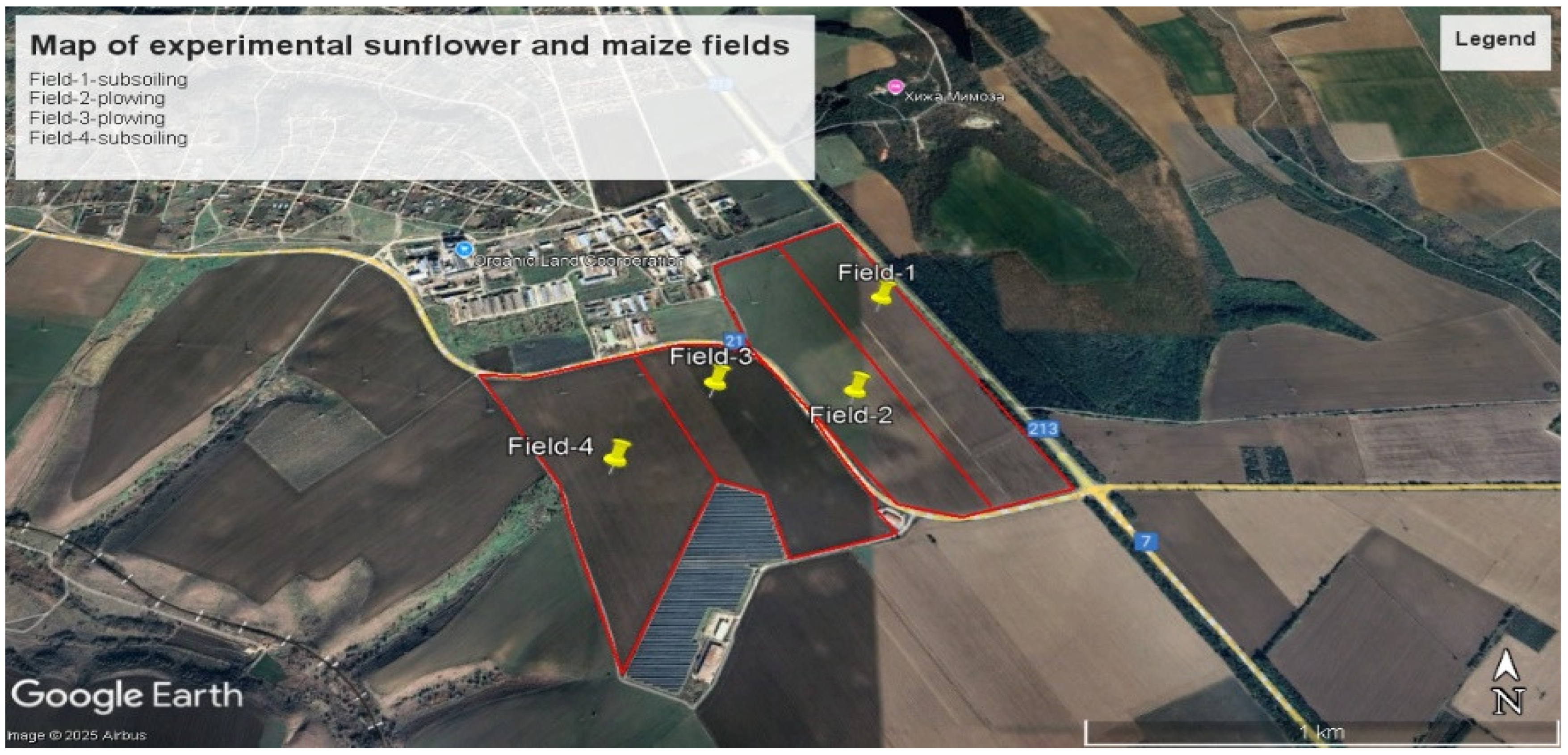
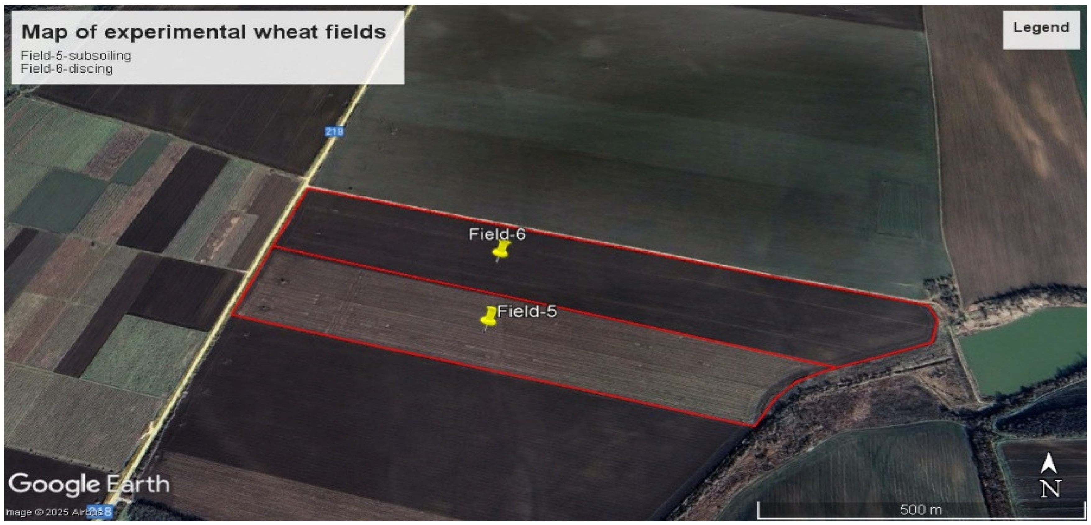
The experimental fields are located within a radius of 3 to 5 km from the village of Kalipetrovo. For the purposes of this study, the fields were designated as Field 1 through Field 6, as shown in Figure 1 and Figure 2. The crop rotation system in the cooperative is dynamic, with different crops cultivated each year according to a rotational plan aimed at preserving soil fertility and reducing pest and disease pressure.

During the 2023–2024 agricultural season, sunflowers were cultivated on both Field 1 and Field 2. On Field 1, subsoiling was implemented as the primary tillage method, while Field 2 underwent conventional deep plowing. Maize was sown on Field 3 and Field 4, with plowing applied to Field 3 and subsoiling to Field 4. Wheat was cultivated on Field 5 and Field 6. On Field 5, subsoiling was employed as a secondary soil preparation technique, whereas Field 6 was managed using disk harrowing.

Field operations were carefully scheduled and performed using the same equipment to ensure uniformity across treatments. On 15 November 2023, subsoiling was conducted on Field 1 to a depth of 50 cm across 30 ha using a Case IH Magnum 340 tractor (Racine, WI, USA) equipped with a Lemken “Karat 9” deep loosening cultivator (Alpen, Germany). On the same date, deep plowing was performed on Field 2 to a depth of 35 cm over the remaining 15.6 ha using the same tractor model.

Similarly, on 15 November 2023, Field 3 was plowed, and Field 4 underwent subsoil deepening, both using the Case IH Magnum 340 tractor with appropriate implements. The identical dates and equipment usage allowed for controlled comparisons of the two tillage techniques under similar soil and weather conditions.

On Field 5, preparatory tillage was carried out earlier in the season. Disk harrowing was performed on 28 September 2023, reaching a depth of 25 cm, using a Väderstad Carrier disk harrow (Väderstad, Sweden) attached to the same Case IH Magnum 340 tractor. Based on operational scheduling and field assessments, Field 6 underwent subsoil loosening to a depth of 27 cm using the Lemken “Karat 9” deep loosening cultivator and the same tractor model.

This experimental setup allowed for a direct comparison of different tillage methods—subsoiling, plowing, and disking—across various crop types and soil conditions while maintaining consistency in mechanization and timing. Such methodological uniformity enhances the reliability of the observed agronomic and soil-related outcomes.

3. Results and Discussion

3.1. The Internet and Generative Models as a Source of Information for Farm Machinery Management

It can be assumed that the amount of information available on the Internet regarding agricultural machinery, technologies, and management is virtually limitless for a single individual to process. Despite conducting searches using carefully selected keywords and phrases, we cannot claim that the results are entirely representative. Therefore, in the following section, alongside general observations, we will highlight selected good practices and useful sources of relevant data.

The first obstacle farmers often encounter is the language barrier. Some specialized terms in this professional field are synonymous, while others—despite having different meanings—are used interchangeably. Such a problem is most often the result of translation from the original language. To some extent, they can be avoided by using multilingual websites. A good example of such a solution is the agricultural machinery specs portal [55], which is available in Polish, English, Spanish, Italian, French, German, Dutch, and Russian. This website focuses on providing essential technical data, including specifications and parameters for agricultural machinery such as agricultural tractors, combine harvesters, and telescopic loaders.

As a result of the withdrawal of some governments from research and testing activities related to agricultural machinery—including in Bulgaria—the availability of information about newly manufactured machines has significantly decreased. Such data are increasingly scarce and often incomplete; see, for example, [56,57].

Naturally, most sources of specific data are from traders and manufacturers. On one hand, these sources can be considered trustworthy, as they have legal responsibilities regarding accuracy and an interest in maintaining a good reputation. Additional advantages include the ability to provide quick and frequent updates, as well as opportunities for direct personal contact. On the other hand, such sources often only highlight the advantages of their products. Measurements are frequently taken under ideal rather than real-world conditions, and objective comparisons with competing products are usually lacking. Furthermore, some sources may be deliberately misleading, for example, due to SEO-driven marketing tactics. This underscores the need for the critical analysis and evaluation of such information—based on logical reasoning, self-reflection, and openness to new perspectives. This approach supports the formulation of well-founded conclusions and decisions based on factual evidence.

From a user perspective, in our opinion, some of the most complete and useful sites for farm machinery management are provided in [58,59]. This data format allows for not only direct use but also the possibility of comparisons and informed choices between closely related purpose machinery.

It is also essential to consider some of the most advanced information retrieval tools available today, particularly large language models (LLMs). In addition to general insights, we will present specific examples of queries/prompts and corresponding responses from some of the more widely used AI-based text and content generation models. The questions vary in scope and specificity, depending on the nature of the information sought after—for example, questions about principles, rules, procedures, or dilemmas requiring a choice.

For example, we started with the following question: How can the Internet and LLMs assist in informing farmers’ decisions in farm machinery management?

Answer: Large language models (LLMs) can assist farmers in making informed decisions about farm machinery management by providing data-driven insights, expert recommendations, and real-time support.

• What is the best farm machinery for my specific needs? LLMs can analyze farm size, crop type, soil conditions, and budget to recommend suitable machinery.
• When should I replace or upgrade my machinery?
• How can I optimize fuel and maintenance costs?
• What are the latest advancements in farm machinery technology?
• How do I troubleshoot common machinery problems?
• Where can I find reliable spare parts and service providers?
• How can I integrate smart farming tools (IoT, drones, GPS) into my existing machinery?
• What are the best practices for machinery storage and seasonal maintenance?
• How do I calculate the ROI of a new machinery investment?
• What government schemes or subsidies are available for farm machinery purchases?

While these responses were relevant, they remained mostly generic. To evaluate the accuracy and utility of LLM outputs, we undertook a basic qualitative and comparative assessment across three dimensions:

• Consistency between models—we compared answers from multiple LLMs to identify discrepancies.
• Alignment with verified data—when possible, answers were compared with known technical specifications or expert sources.
• Practical relevance and completeness—were the responses applicable, specific, and detailed enough to support decision-making?

As a quantitative example, we tested the response to the question: “What is the throughput of the CASE IH 2388 combine harvester (t/h)?”

The results are summarized in

Table 1. Throughput of CASE IH 2388, t/h, according to two LLMs.

Crop	Wheat	Corn/Maize	Canola/Rapeseed	Sunflower	Soybean
1. LLM	35	30	18–25	20–28	25
2. LLM	22–28	25–35	12–18	15–20	18–24

.

The variation in output values was notable. To verify the data, we asked for sources, but the models could not provide any citations. A typical reply was: “I don’t have specific citations for the throughput data I provided… this information wasn’t drawn from formal published sources”.

This raised concerns about the verifiability and reliability of the generated information. In contrast, conventional sources such as technical manuals, field trials, or manufacturer documentation are more dependable.

Another evaluation case involved the prompt:

“If a fertilizer spreader has a working width of 12–42 m and a speed up to 8 km/h, how to select the right width?”

The LLM’s response listed key factors: field shape, terrain, tractor power, wind, etc., and concluded that the optimal working width should be selected based on field tests. While accurate, the advice was too general and not feasible in pre-purchase scenarios, where testing is not yet possible. This highlighted a lack of contextual depth and cost-awareness in the response.

We also tested LLMs with complex tasks such as crop rotation planning or machine selection under economic and agronomic constraints. Some models labeled the tasks as unsolvable, while others provided low-quality or contradictory answers. Despite iterative prompt refinement, human reasoning was still required to obtain practical solutions. This suggests that while LLMs offer support, human-in-the-loop validation remains essential.

Furthermore, we observed hallucinations—fabricated responses that appeared plausible but were inaccurate. For instance, fictitious citations, overconfident conclusions, and misinterpreted technical parameters were noted. This underscores the need for a systematic accuracy verification process when integrating LLM outputs into decision-making.

Lastly, we found that LLMs and search engines lacked robust information on two crucial categories:

⮚

Quality of machine work (e.g., coverage uniformity, loss rates);

⮚

Reliability and durability under specific farm conditions.

These indicators are critical but often absent from AI-generated responses, reinforcing the importance of on-farm studies and experiments.

3.2. Information at First Hierarchical Level

As was mentioned in the Section 2 “Material and Methods”, any significant change in crops, areas, crop rotation, technologies, and tools regarding their implementation should be modeled in advance. Let us start with base or primary tillage plowing. To decide when to plow, naturally, we first have to take into account the crop, the predecessor, whether it is heavy or light soil, and whether the goal is loosening or simply preparing the soil for sowing. For the subsequent winter after maize has been planted on moderately heavy soil, the expected field capacity and fuel consumption for loosening and inverting the soil are presented in

Table 2. Segment of the spreadsheet model representing the first hierarchical level of farm machinery management. The figure illustrates the calculated field capacity (dka/shift) and fuel consumption (g/dka) for various agricultural units comprising seven different tractors and two types of plows (Lemken Vario Diamant 6 + 1 and Lemken Vari-Opal 5).

Agricultural Operations	Power Unit: Tractor, Self-Propelled Machine, Track		First Machine		WCM	g	Initial Solution		Final Solution
	Brand, Model, Modification	Traction System: 1—2WD 2—MFDW 3—4WD 4—Track	Brand, Model, Modification	Working Width, m	dka/shift	g/dka	Utilization of Speed	Utilization of Power	Utilization of Speed	Utilization of Power
				B1			ΔV	Δη	ΔV	Δη
Autumn Plowing to a depth of 32 cm	CASE IH Magnum 340	2	Lemken Vari-Diamant 6 + 1	2.2	137	2160	0.00	0.07	0.00	0.02
	New Holland T7.315 (Turin, Italy)	2		2.2	128	2070	0.00	−0.05	0.18	0.00
	CASE IH Magnum 335	2		2.1	131	2170	0.00	0.04	0.00	0.03
	Deutz Fahr Agrotron 260 (Lauingen, Germany)	3		1.8	101	2230	0.00	−0.06	0.28	0.03
	CASE IH PUMA 210	2		1.8	89	1930	0.00	−0.05	0.58	0.09
	CASE IH Maxxum 140	2		1.8	69	1720	0.00	−0.12	1.08	0.05
	CASE IH Magnum 340	2	Lemken Vari-Opal 5	1.8	112	2340	0.00	0.42	0.00	0.19
	New Holland T7.315	2		1.8	112	2200	0.00	0.35	0.00	0.09
	CASE IH Magnum 335	2		1.8	112	2290	0.00	0.40	0.00	0.16
	Deutz Fahr Agrotron 260	3		1.5	94	2390	0.00	0.19	0.00	0.04
	CASE IH PUMA 210	2		1.3	81	2180	0.00	0.10	0.00	0.06
	CASE IH Maxxum 140	2		1.3	64	1900	0.00	−0.05	0.58	0.02

.

The calculations are based on data related to terrain and soil properties, which directly influence motion resistance, the tractive coefficient, and the slip of the agricultural unit. The different colors of cells have to make easy enter and visual analysis.

The initial evaluation of machinery performance is shown in columns Initial Solution “ΔV” and “Δη”, which display the reserves of speed and current engine power, respectively. Values highlighted in red indicate power shortages, signaling potential overload or an inability to operate effectively. To ensure optimal performance, it is proposed to reduce the working width of the plow; these reductions are indicated in red in column “Working Width, m B1”. This adjustment guarantees sufficient power when using the Lemken Vario Diamant 6 + 1 plow, with the final optimized solutions presented in columns Final Solution “ΔV” and “Δη”.

For tractors with a lower engine power—specifically those listed in rows for CASE IH Magnum 340, New Holland T7.315, and CASE IH Magnum 335 with Lemken Vari-Diamant 6 + 1—the required working width reduction is more significant. When using the smaller Lemken VARI-PAL 5 plow, only the last tractor CASE IH Maxxum 140 with Lemken Vari-Opal 5 requires such a reduction. Additionally, to maintain consistent plowing depth and quality with the larger plow, a slight to moderate reduction in forward speed is recommended for some agricultural units, as indicated by positive values in column Final Solution “Utilization of Power”.

Similarly, a plowing simulation was performed for spring preparation before sowing corn and sunflowers, targeting a soil depth of 22 cm. For the crops grown on the farm—winter wheat, winter barley, winter rapeseed, sunflower, corn, and rapeseed—tractors are not needed for other operations, which simplifies prioritizing agricultural units based on field capacity and fuel consumption. However, the situation differs for plowing after harvesting crops with shorter growing periods. In such cases, decision-making requires careful consideration of competing crop schedules within overlapping time windows.

This is the case with the harvest, the simulation of which is shown in

Table 3. Segment of the spreadsheet model for the first hierarchical level of farm machinery management. The figure presents calculated field capacity (dka/shift) and fuel consumption (g/dka) for harvesting operations involving four major crops: winter wheat, winter rapeseed, maize (corn), and sunflower.

Agricultural Operations	Power Unit: Tractor, Self-Propelled Machine, Track	First Machine	WCM	g	Final Solution		Residue-to-Product Ratio	Fertilization, Spraying, Sowing Rate, Yield, t/dka
	Brand, Model, Modification	Brand, Model, Modification	dka/shift	g/dka	Utilization of Speed	Utilization of Power
					ΔV	Δη
Summer—harvesting of winter wheat	New Holland CX 8.90	New Holland 24V Rigid Grain Header	231	1340	0.00	0.56	1.4	0.37
	CASE IH Axial Flow 8120	Case IH 2020	208	1320	0.00	0.53
	CASE IH 2388	Case IH 3020	268	750	0.00	0.25
Autumn—harvesting of maize/corn	New Holland CX 8.90	New Holland Corn Header	192	980	0.00	0.80	1.1	0.162
	CASE IH Axial Flow 8120	Case IH 2083	147	1160	0.00	0.80
	CASE IH 2388	Case IH 3200	199	730	0.00	0.73
Summer—harvesting of sunflower	New Holland CX 8.90	New Holland Sunflower Header	160	1230	0.00	0.79	2.2	0.20
	CASE IH Axial Flow 8120	Case IH Sunflower Header (Low-Cut)	128	1340	0.00	0.79
	CASE IH 2388	Case IH Sunflower Header	132	1090	0.00	0.73
Summer—harvesting of rapeseed	New Holland CX 8.90	New Holland Grain Draper	160	1660	0.00	0.69	1.7	0.24
	CASE IH Axial Flow 8120	Case IH FlexDraper™	220	1200	0.00	0.59
	CASE IH 2388	Case IH FlexDraper™	230	830	0.00	0.44

.

In this figure, two additional columns “Residue-to-Product Ratio” and “Fertilization, Spraying, Sowing Rate, Yield” have been added to the previous calculation table to determine the mass of plant material entering the combine harvester. This input directly influences the throughput capacity of the threshing system. This parameter includes not only the grain yield but also the proportion of material other than grain (MOG), which varies depending on the crop—such as small grains (e.g., wheat, rapeseed) or row crops (e.g., maize/corn, sunflower). These data were derived from both on-farm yield records and standardized coefficients obtained from technical documentation for the specific harvester models. The different colors in the table facilitate their visual analysis. For example, the green background refers to input data, the red and gray - to intermediate results for the field-only and the entire machine complex operation phases, respectively, and the white - to the final results.

Although the diversity of combine harvesters on the farm is not as extensive as that of tractors, inconsistency in machinery fleet renewal policies poses significant challenges for effective farm machinery management. For instance, the varying field capacities of different grain harvesters and headers can interrupt the optimal flow of the harvesting process and complicate synchronization with grain transport logistics.

The combines currently in use have been properly selected to cope with the highest expected grain yields and high straw-to-grain ratios in winter wheat. However, the effective utilization of engine power during these operations—reflected in column Final Solution “Utilization of Power”—is significantly lower than during power-intensive tasks such as plowing. This discrepancy becomes even more pronounced when harvesting lower-yield crops like maize, sunflower, and rapeseed, where engine loading drops further.

Due to the uneven terrain and field configurations on the farm, increasing header width is not a feasible solution for improving capacity. Likewise, increasing the forward working speed is limited by the resulting rise in grain losses and compromised harvesting quality. This highlights the trade-off between throughput and harvest precision.

Another critical factor affecting harvesting efficiency is the dynamic variation in motion resistance caused by the increase in grain mass as the hopper fills. A fully loaded combine experiences substantially greater resistance than when operating empty. Moreover, fluctuations in grain and straw moisture content—common in real-world harvesting conditions—demand adaptive engine power to maintain optimal threshing quality. This necessitates an increased engine power reserve, especially under high-moisture or heavy weed conditions.

Overall, the data presented in Table 3 emphasize the complex interplay between machine specifications, terrain characteristics, and crop-specific requirements. Proper interpretation of these results helps inform decisions regarding machinery allocation and scheduling, ultimately contributing to more efficient harvesting operations and reduced grain losses.

It is important to emphasize that the performance of harvesting units is not solely determined by the engine power of the combine. A significant influence is exerted by both the type and width of the header, as well as the capacity and efficiency of the threshing unit. These components dictate the combine’s ability to process biomass effectively under varying field conditions.

Additionally, the level of weed infestation and the general condition of the plants at the time of the harvest play a critical role in determining the maximum feasible harvesting speed. Increased weediness or uneven ripening can reduce working speed, increase the load on the threshing system, and increase fuel consumption per hectare.

Another crucial factor is the time efficiency of the harvesting process, which typically ranges between 60% and 75%. Unlike primary tillage, harvesting efficiency is not solely dependent on field conditions and machinery performance. It also depends on the availability and scheduling of supporting transport vehicles, the condition of farm roads, field access logistics, and even general traffic conditions within the farm. All these variables affect idle time and transport delays.

Therefore, the realistic value used for time efficiency in the calculations of field capacity and fuel consumption has a substantial impact on the final operational assessments. Underestimating or overestimating this factor may lead to poor planning and bottlenecks during peak harvesting periods. The approach used in this study assumes conservative estimates based on historical farm data, combined with manufacturer benchmarks and standard engineering references to ensure practical relevance.

3.3. Information at Second Hierarchical Level

To evaluate and select the most suitable combination of different machines and their numbers, sufficient simulations were performed. The calculation process was terminated when high productivity and, consequently, reduced idle time were achieved. Below is the outcome for the simulation of harvesting by a machinery complex composed of two grain harvesters, without an intermediate bunker, three vehicles, and one storeroom with a truck scale and a loading conveyor.

The total idle time, $Ti,$ and operating time, $T02,$ are given below:

• Grain harvesters:

For number 1—$Ti$ = 0:31 h and $T02$ = 9:06 h; for number 2—$Ti$ = 0:27 h and $T02$ = 9:11 h; and total idle time = 0:57 h.

• Vehicles:

For number 1—$Ti$ = 1:50 h and T02 = 9:15 h; for number 2—$Ti$ = 1:54 h and $T02$ = 9:08 h; for number 3—$Ti$ = 2:46 h and $T02$ = 6:30 h; and total idle time = 6:14 h.

Storehouses: for number 1—$Ti$ = 7:00 and $T02$ = 9:38 h.

• Amount of harvested product and general indicators for the complex:

For grain harvester number 1—142 m³.

Area from which the product was harvested—148 decares.

Productivity of machinery complex—0.256 m³/min.

Machine hours for 1 m³ of product—0:05 h.

Idle time per unit capacity—0:03/m³.

Process continuity coefficient—0.73.

Utilization productivity of the harvesting equipment—0.94.

Utilization productivity of the vehicles—0.76.

When the machinery complex includes intermediate bunkers, relative data is presented with text and numbers. The summary indicator of the complex’s performance is the process continuity coefficient. The goal is to make it as close to 1 as possible. Naturally, this should not be carried out with an unjustified increase in the number of machines and service personnel involved.

To determine the expected time efficiency, downtime should also be taken into account when a resource is unable to operate or be productive (for example, because of breakdowns, failures, and other unexpected issues).

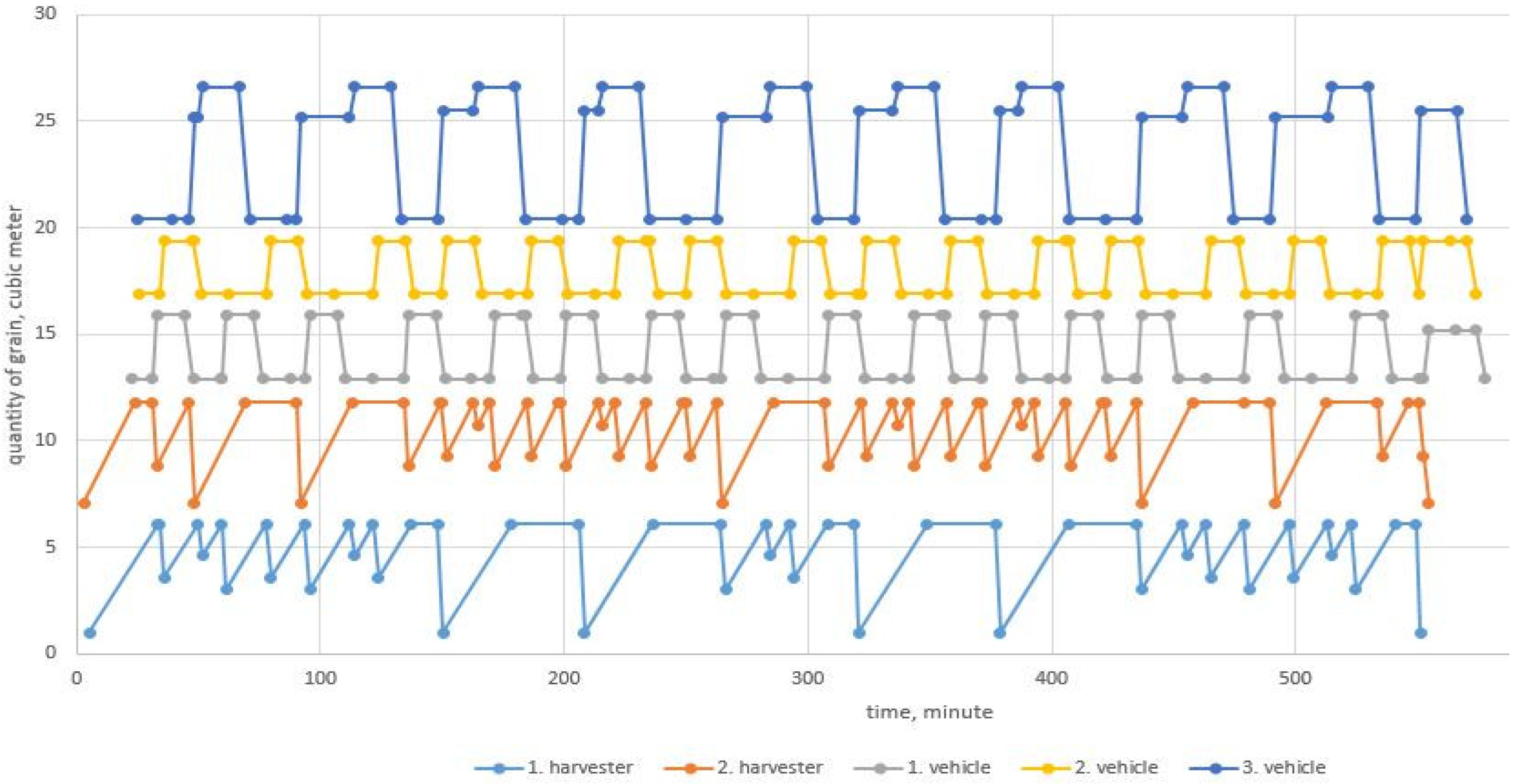
Additional information about the interaction between individual machines is provided through visualization. A diagram shows the change in the amount of material in hoppers, bodyworks, tanks, or machines’ volumes for harvested products from the field or for products sowed, sprayed, or spread in a field during a shift.

It is possible to see that more vehicles arrived in the field than combines—see Figure 3. For example, combine number 2 had to maintain a filled hopper until all the product was unloaded into vehicle 3. Another vehicle—series 5—had larger bodywork so had to wait to be filled two times before it started traveling back to the storehouse. Also, the same vehicle had a capacity two times larger than that of the other two vehicles.

Some components of the machinery complex make presenting of the interaction between harvesters and vehicles difficult. Other scales and ordinates are required to depict intermediate bunkers and, in particular, storehouses with large volumes. At the same time, mobile or stationary field bins and dump trailers or those with an unloading screw conveyor can prolong transport times. It is a good idea to only implement time intensification for transportation. Regrettably, due to road restrictions, this time intensification did not prove acceptable for this particular farm.

In a similar way, the interaction between machines for operations such as sowing, spraying, and fertilizing can be simulated and presented—see Figure 4.

The fertilizer spreaders are mounted and have a small, approximately equal volume. This is the reason they achieve almost perfectly coordinated work in terms of quantity and time. For specific conditions, we were unable to use generated quasi-random values. The reason for this is that the samples were not representative and a small number of the complex’s components led to the distortion of the results.

In addition to the indirect method of transporting agricultural goods, the direct loading, transport, and operation of seeding, spraying, and fertilizing machines (for micronutrient fertilizers) are also possible. This minimizes idle time due to inconsistency and, in some cases, requires fewer technical and human resources. Important preconditions for applying this method are small quantities of product per unit area, short transport distances, and possibly significantly higher transport speeds than the working speed. To make the correct choice in each specific case, the previously discussed spreadsheet with some modifications can be used.

Table 4. Segment of the spreadsheet model for the second hierarchical level of farm machinery management. The figure presents the calculated field capacity (dka/shift) and fuel consumption (g/dka) for agricultural operations involving fertilization and spraying, incorporating transport distances and application rates.

Agricultural Operations	Power Unit: Tractor, Self-Propelled Machine, Track	First Machine	Field Capacity	Fuel Consumption	Field Capacity	Fuel Consumption
	Brand, Model, Modification	Brand, Model, Modification	dka/shift	g/dka	dka/shift	g/dka
Autumn—back to farmyard empty	CASE IH JX95	PT-10
Autumn—to field full	CASE IH JX95	PT-10	105	869
Autumn—manure spreading with 2 t/dka	CASE IH JX95	PT-10	53	1539	53	1539
Spring—back to farmyard empty	Berthoud BRUIN 2000 (Belleville sur Saône, France)
Spring—to field full	Berthoud BRUIN 2000		3752	46
Spring—spraying with 30 l/dka	Berthoud BRUIN 2000		1777	86	1777	86
Spring—back to farmyard empty	CASE IH Maxxum 140	AMAZONE UX 4200
Spring—to field full	CASE IH Maxxum 140	AMAZONE UX 4200	1420	76
Spring—spraying with 30 l/dka	CASE IH Maxxum 140	AMAZONE UX 4200	710	136	710	136
Spring—back to farmyard empty	CASE IH Maxxum 140	FC-3.2
Spring—to field full	CASE IH Maxxum 140	FC-3.2	1417	71	1417	71
Spring—spraying with 30 l/dka	CASE IH Maxxum 140	AMAZONE UX 4200			1418	50

presents the results of calculations related to manure spreading and solution spraying operations. Two additional columns—B and C—were introduced to reflect the distance from the farmyard to the field and the fertilization, spraying, or sowing rate per decare, respectively. These values are crucial inputs for accurately modeling time and fuel requirements under realistic field logistics.

In first 3 rows with CASE IH JX95, the field capacity of a tractor with a trailer for manure spreading is calculated. Intermediate results for transport and fertilization are presented in columns with gray background, while the final aggregated values for loading, transport, and spreading are shown in the last two columns in the right. The resulting field capacity for manure application is relatively low due to the heavy nature of the material and frequent transport cycles.

However, given the specific natural and climatic conditions of the farm, the impact of moderate delays in organic fertilization on overall crop returns is minimal. For this reason, alternative transport strategies (e.g., using trucks or additional trailers) were not modeled in detail.

In contrast, for solution spraying, timeliness is significantly more critical. Delays in application, especially for plant protection products, can lead to substantial yield losses. Although there is limited empirical data on a strict timeliness coefficient for spraying, the importance of completing the operation within a narrow time window is well-documented in the agronomic literature.

To address this, multiple operational strategies were simulated. The use of self-propelled sprayers—simulated in rows Berthoud BRUIN 2000—offers a significant increase in productivity (e.g., cell “1777”), enabled by faster working speeds and reduced time for maneuvering. The numbers presented in bold refer to the final characteristics of the machine complexes. These units also benefit from extended working hours facilitated by GPS guidance and precision control systems, making them particularly effective under time-sensitive scenarios.

For comparative purposes, a conventional approach using a tractor and mounted sprayer is analyzed (cell for “Spring—spraying with 30 l/dka” with CASE IH Maxxum 140 and AMAZONE UX 4200 – “770”), showing markedly lower field capacity. Additionally, a hybrid strategy is simulated, where the spraying solution is transported to the field using a tractor and tank trailer, and the spraying is performed by another tractor using the same sprayer (the two right cells of penultimate two lines). The number are shown in bold as In this case, at the tested transport distance, the field capacities of the transport and spraying units are very similar (1417 and 1418 decares per shift, respectively), resulting in high process efficiency.

For different distances or higher spraying rates, alternative ratios between the transport and spraying units may be optimized to maintain coordination. A key prerequisite for effective synchronization is that the higher field capacity should be a multiple of the lower one, ensuring continuous operation without idle time. Failing to meet this condition would result in a lower process continuity coefficient, reducing overall operational efficiency.

These calculations allow farm managers to select the most efficient spraying method based on field size, available machinery, and time constraints—ultimately improving productivity and reducing input costs.

3.4. Information at Third Hierarchical Level

The information obtained by searching publicly available sources and from the previous levels is used as a basis for entering data at the level of machine and fleet park management. Naturally, at this level, the set of possible solutions is the largest. Accordingly, their study is very laborious and time-consuming. Therefore, only selected results are presented below to demonstrate the decision-making logic and the system’s integrative capacity. A possible solution for the farm in Kalipetrovo is the use of a utility tractor, with the following main characteristics: 81 kW, MFDW, and 4100 kg mass. This configuration is suitable for most operations—tillage, plowing, seeding, fertilizing, spraying, row cultivation, and haulage—but not for harvesting.

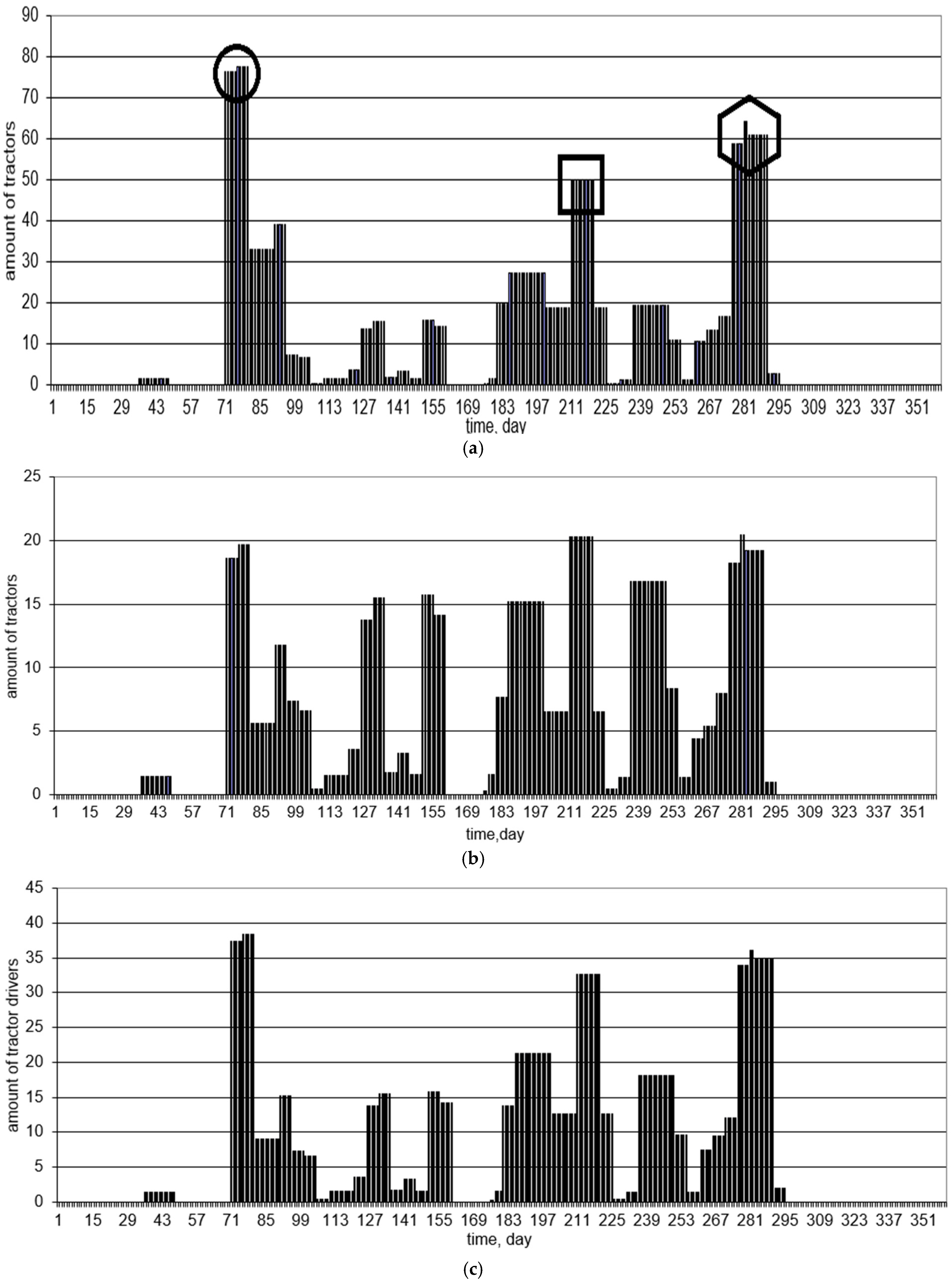
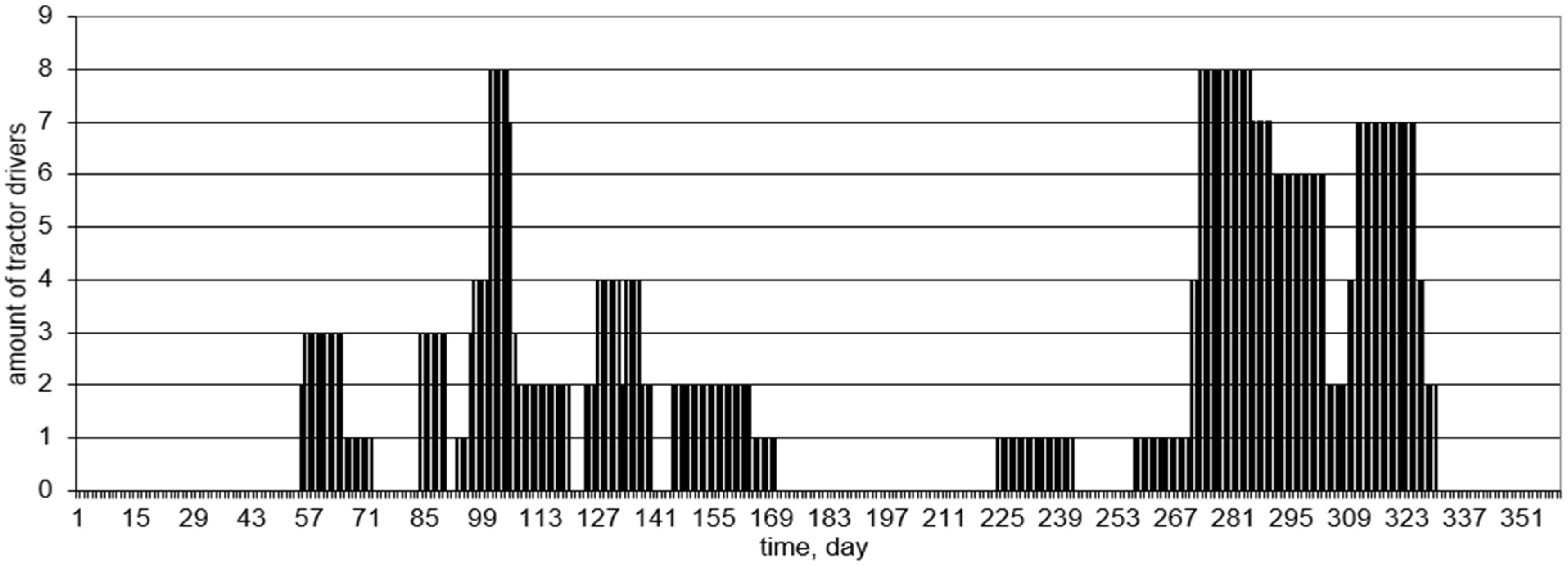
Using field capacity and fuel consumption data from the operational level, an initial estimate of the machinery demand is generated—Figure 5a. Peaks in tractor demand are identified (highlighted with shapes), and time windows are adjusted based on cursor positioning to align with these peaks. Modifications are then made to working hours, shift numbers, and workdays. The process concludes if such changes are no longer possible or do not reduce the quantity of relevant resources—Figure 5b.

As a result, the number of tractors needed was reduced by 3.5 times, and the number of tractor drivers was halved. If during periods of peak demand other tractor drivers are temporarily hired, it is possible to reduce their number to the number of tractors shown in Figure 5c.

Fleet scheduling, especially when resources cannot be renewed easily, is more complex. This complexity arises from regulatory limitations, banking policies, and the underdeveloped used-machinery market in Bulgaria. The wide variety of machines and environmental factors, along with integer solution requirements, further complicate optimization.

Despite these challenges, a feasible schedule was created (Figure 6 and Figure 7), showing integer-based solutions for both equipment and personnel deployment. The approach demonstrates how hierarchical information—starting from physical models (operational level) to machine coordination (logistics level) and culminating in strategic fleet planning—can be successfully integrated.

It turned out that tractors are sufficient for the eventual implementation of soil loosening. At the same time, increasing the number of disk harrows by one will allow for deep loosening up to 25 cm in an acceptably short time. A favorable condition for this on the Kalipetrovo farm is the availability of both general-purpose tractors and agricultural tractors with large capacities and weights.

Naturally, the potential for deeper soil cultivation is associated with a significant increase in fuel consumption, as illustrated in Figure 6. Detailed data on daily fuel requirements can be utilized to adjust fuel storage capacities accordingly. For instance, storage systems must allow for adequate diesel settling time—at least three days after delivery—to enable sediment and water to separate and settle at the bottom. Additionally, the approach provides an opportunity to optimize the fuel delivery schedule, ensuring continuous and efficient field operations.

It is worth noting that the actual employment of tractor drivers on the farm may be lower than projected in the earlier scenario involving a single primary tractor. Nevertheless, a positive outcome for the revised configuration is the observed 9% increase in the average tractor engine power, contributing to improved operational efficiency. While their practical utility has been demonstrated, we acknowledge—through self-critical reflection—that these procedures could be further developed into a comprehensive decision support system. Moreover, establishing a database that captures compatibility relationships among tractors, implements, agricultural operations, and crops would significantly enhance the applicability and scalability of this approach.

Similarly, the number of tractor drivers would increase in October and November, when, as a general rule, most of them are not engaged in fieldwork—see Figure 7.

Notable discrepancies may arise between the expected results derived from the modeling of machinery operations and their actual performance across different hierarchical levels. In such cases, it is advisable to critically assess the underlying models, computational procedures, and, most importantly, the empirical data. To clarify these differences, simple field experiments—along with their representation through regression analyses—can serve as effective validation tools.

3.5. Key Results from This Study

This study led to several important outcomes that illustrate the effectiveness of the proposed approach. Through the detailed scheduling and adjustment of work shifts, the required number of tractors was reduced by 3.5 times. This optimization was accompanied by a 50% reduction in the number of tractor drivers, achieved through better labor planning and allocation. To address peak workload periods, the inclusion of temporary labor proved effective in aligning workforce capacity with machinery availability.

Additionally, the optimized configuration resulted in a 9% increase in the average engine power of tractors compared to the baseline solution, enhancing overall field performance. Deep soil loosening operations were successfully completed within the available operational time by incorporating an additional disk harrow, demonstrating a targeted improvement in equipment deployment.

Finally, the development of seasonal schedules for both fuel consumption and tractor driver engagement provided actionable insights that can support more efficient planning for fuel deliveries and labor contracts. These integrated results highlight the value of this hierarchical approach in improving agricultural machinery management under real-world constraints.

4. Practical Implications

The developed informational support approach offers several tangible benefits for farm managers and practitioners:

✓

Enables resource optimization through detailed scheduling and equipment matching.

✓

Assists in investment decisions related to machine purchases or replacements.

✓

Enhances the resilience of operations to weather variability through flexible planning.

✓

Can be used as a training and educational tool for students in agricultural engineering.

✓

Offers a low-cost digital alternative to expensive farm management platforms, especially in regions with limited access to advanced systems.

Its implementation requires basic Excel skills and structured data, making it feasible for medium-scale farms with limited digital infrastructure.

5. Study Limitations

Despite these encouraging results, several limitations should be acknowledged:

✓

The data, soil, climate, and machinery setup are specific to the Kalipetrovo region and may not fully represent conditions elsewhere.

✓

Although the simulation results matched field outcomes relatively closely, full-scale multi-year validation is still lacking.

✓

Some dynamic factors like weather changes, mechanical failures, and labor constraints were only partially considered or idealized.

✓

This study relies primarily on spreadsheets and manual inputs rather than real-time IoT-based data collection, which could enhance accuracy and automation.

6. Conclusions

This study underscores the abundance of online information about agricultural machinery while highlighting the risks of misinterpretation due to incomplete, outdated, or biased sources. This underlines the need for critical thinking and evidence-based decision-making when managing mechanized field operations.

Our main contribution is the development and application of a hierarchical decision-making framework that integrates three levels:

⮚

Operational—focusing on field capacity and fuel efficiency;

⮚

Logistic—addressing machine coordination and idle time reduction;

⮚

Strategic—optimizing fleet composition and labor allocation.

The case study in Kalipetrovo demonstrated that significant resource savings can be achieved—such as a 3.5-fold reduction in tractor requirements and improved workload distribution—by applying structured information management and scheduling strategies. Figure 3, Figure 4 and Figure 5 illustrate how information flows from technical data to strategic planning, validating the hierarchical model’s capacity to support integrated machinery decisions.

This approach successfully bridges the data gap by combining expert knowledge, publicly available online information, and manually structured datasets into an adaptable decision-making tool. It also represents a low-cost alternative for farms that lack access to commercial precision agriculture platforms.

Future research directions include the following:

The incorporation of economic modeling, enabling cost–benefit analysis, investment evaluation, and machinery depreciation planning;

The development of AI-based decision support systems with compatibility databases for machines, operations, and crops;

Experimental studies focused on sowing quality and output variability with different machinery and technologies;

The integration of sustainability metrics, including environmental impact and labor welfare;

The gradual adoption of IoT-based real-time monitoring to refine models and reduce manual inputs.

We also acknowledge that a robustness analysis using sensitivity or scenario testing would provide additional confidence in the results.

Future work may include the integration of empirical datasets and comparative field trials to validate and refine the model under a broader range of conditions.