Pears Internal Quality Inspection Based on X-Ray Imaging and Multi-Criteria Decision Fusion Model

Abstract

Pears are susceptible to internal defects during growth and post-harvest handling, compromising their quality and market value. Traditional detection methods, such as manual inspection and physicochemical analysis, face limitations in efficiency, objectivity, and non-destructiveness. To address these challenges, this study investigates a non-destructive approach integrating X-ray imaging and multi-criteria decision (MCD) theory for non-destructive internal defect detection in pears. Internal defects were identified by analyzing grayscale variations in X-ray images. The proposed method combines manual feature-based classifiers, including Local Binary Pattern (LBP) and Histogram of Oriented Gradients (HOG), with a deep convolutional neural network (DCNN) model within an MCD-based fusion framework. Experimental results demonstrated that the fused model achieved a detection accuracy of 97.1%, significantly outperforming individual classifiers. This approach effectively reduced misclassification caused by structural similarities in X-ray images. The study confirms the efficacy of X-ray imaging coupled with multi-classifier fusion for accurate and non-destructive internal quality evaluation of pears, offering practical value for fruit grading and post-harvest management in the pear industry.

1. Introduction

Pears are susceptible to physiological diseases, bacterial infections, pest damage, collisions, and other factors during growth, storage, and transportation, which may result in defects such as corking, mold, insect infestation, and bruising [1,2,3], leading to a decrease in fruit quality. Traditional detection methods—manual inspection and physicochemical analysis—are often inefficient, subjective, destructive, or time-consuming. These limitations highlight the need for non-destructive internal quality inspection methods. Improving detection accuracy is essential for enhancing product consistency and meeting market demands for high-quality, differentiated agricultural produce, which in turn can boost the economic value of China’s pear industry.

Internal quality refers to the intrinsic characteristics of the fruit that are not visible from the outside, including internal defects, flesh texture, firmness, and chemical composition. This study focuses on detecting internal defects in pears—such as impact damage, woolliness, insect infestation, corking, and rot—which directly affect edibility and market value. Common non-destructive detection technologies include hyperspectral imaging, X-ray, NIR, electronic nose, and NMR, each with varying effectiveness and limitations. Hyperspectral imaging provides continuous spectral data across a wide wavelength range, offering higher resolution and richer detail than multispectral techniques, with coverage spanning dozens to hundreds of discrete wavelengths [4]. Zhang et al. used the CARS algorithm to select characteristic wavelengths and construct a GS-SVM model, achieving an accuracy of 96.77% for defect detection in peaches [5]. However, despite its comprehensive detection capabilities, hyperspectral imaging faces challenges such as band redundancy, high inter-band correlation, complex data processing, and slow image acquisition—limiting its suitability for rapid, real-time applications. The electronic nose mimics the human olfactory system through sensors and pattern recognition technology [6]. Fruits emit distinct volatile gases during growth and decay, which can be analyzed to assess internal quality. Gila et al. combined electronic nose sensors with pattern recognition to classify olive oil quality, achieving 90.2% accuracy [7]. Electronic nose technology offers real-time, low-cost, and rapid detection, but remains immature and prone to environmental interference and sensor sensitivity issues, leading to potential inaccuracies. Near-infrared spectroscopy (NIR) enables rapid analysis of chemical and biological samples by capturing spectral features that reflect their composition and structure [8,9]. Kang et al. developed an NIR detection method using IWOA-LSSVM, achieving determination coefficients of 0.8667 and 0.8216 for predicting soluble solids and vitamin C in cherry tomatoes [10]. However, NIR suffers from limited sensitivity, poor detection of trace components, weak anti-interference performance, and insufficient technological maturity. Nuclear magnetic resonance (NMR) detects molecular structure by analyzing nuclear spin behavior in a magnetic field, enabling imaging-based assessment of fruit internal quality. Qiao et al. used this technology to examine blueberry rot disease [11]. NMR relaxation analysis showed increased transverse relaxation time in decayed fruit, confirming its effectiveness. However, despite its high imaging accuracy, practical application remains limited due to technical and operational challenges.

X-ray non-destructive testing assesses internal fruit quality by detecting density-based differences in X-ray attenuation. X-ray CT further provides 3D imaging that visualizes internal structural variations based on these density contrasts. Arendse et al. used CT technology to characterize and quantify the internal structure of pomegranates and estimate their volume [12]. The method accurately segmented pomegranate structures and estimated component volumes, with results comparable to destructive testing, confirming X-ray CT’s suitability for internal morphological analysis and volume estimation in fruits. Unlike X-ray CT’s 3D imaging, standard X-ray imaging produces 2D projections where density variations are superimposed. Despite this, it effectively detects internal defects and enables rapid imaging (~10 s for multiple fruits), making it ideal for real-time, online inspection. Thomas et al. used X-ray imaging to detect weevil infestation in mangoes, where infected areas appeared darker than healthy tissues, demonstrating the technique’s effectiveness for identifying internal fruit defects [13]. Matsui et al. developed an automated detection system for internal decay in Hass avocados by combining X-ray imaging with deep learning-based semantic segmentation [14]. Using an enhanced U-Net++ model, they achieved 98% accuracy in detecting stem-end rot and pulp decay in avocados, even under low contrast, offering a reliable and efficient non-destructive inspection method with reduced false positives.

Thomas et al. used cGANs to generate synthetic CT images of healthy and damaged pears, demonstrating their potential in detecting internal bruises and cavities under limited training data [15]. Munera et al. applied X-ray imaging and random forest classification to detect heart rot in pomegranates, achieving 93.3% accuracy—significantly outperforming manual inspection (66.7%)—and proving highly effective for early-stage disease detection [16]. Tempelaere et al. used X-ray radiography with deep learning to detect pear defects, employing a cGAN-based method to generate synthetic CT images, enhance training data, and improve segmentation of internal browning and cavities [17]. Nugraha et al. developed a non-destructive porosity mapping method using X-ray CT, correlating grayscale values with tissue porosity. Reference scans and image normalization improved 3D accuracy and adaptability across various fruit and vegetable types [18]. Marinho et al. used digital radiography and CNNs to detect parasitism in fruit fly pupae. The Xception model achieved 99.33% accuracy and enabled non-invasive identification of all five parasitic stages—far outperforming traditional 16-day biological methods [19]. Yu et al. used X-ray scanning to detect freezing injury in pears, finding that freezing-induced cavities had higher grayscale values. They observed a negative correlation between damage area and temperature, and a monotonic grayscale increase with longer freezing duration [20]. Tim et al. used X-ray CT and SVM classification on 2D slices to detect internal pear defects, achieving over 90% accuracy. Feature importance analysis identified key discriminative traits, highlighting the method’s potential for non-destructive quality assessment [21]. Raza et al. proposed the FEViT model, combining vision transformers with CNN modules to classify citrus freshness from X-ray images, achieving 99.25% accuracy—outperforming standard ViT models [22]. Joseph et al. combined X-ray CT with spatially resolved spectroscopy to assess pear porosity, finding a strong linear correlation with scattering coefficients at 760 and 835 nm, demonstrating the potential of optical methods for rapid, porosity-based fruit sorting [23].

While spectral imaging techniques offer detailed chemical information, they are limited by surface dependency, complex analysis, and slow processing. In contrast, X-ray imaging is fast, non-destructive, and capable of detecting deep internal defects by capturing density-based grayscale variations, making it more practical for large-scale fruit inspection. With its maturity and robustness, X-ray technology—originally developed for medical use—offers high accuracy and strong anti-interference capabilities, making it well-suited for internal fruit quality assessment. This study adopts X-ray imaging as the core method for inspecting pears.

In recent years, ensemble learning has garnered significant attention in defect detection tasks due to its ability to leverage multiple models’ strengths while mitigating individual biases. Techniques such as bagging, boosting, and stacking have been widely used to improve robustness and accuracy. Pan et al. developed a hybrid ensemble model combining ResNet, ResNeSt, and attention mechanisms, achieving 99.70% accuracy on the WM-811k dataset—significantly outperforming individual models and highlighting the strength of ensemble methods in complex defect detection [24]. Raei et al. used a U-Net with ResNet-34 backbone to classify irrigation systems from high-resolution images, achieving up to 86% accuracy and demonstrating deep learning’s effectiveness in complex agricultural image analysis [25]. Ferdousi et al. developed an AI-based defect detection system for rail surfaces, integrating machine vision and deep learning, and achieved 97.3% accuracy under diverse environmental and lighting conditions [26].

Ensemble learning has also been effectively applied in agricultural imaging for fruit quality assessment. Ramakrishna et al. proposed a real-time ensemble model combining VGG16, VGG19, ResNet, and InceptionResNetV2 for fruit freshness classification, achieving over 98% accuracy. Integrated into a Streamlit-based tool, the model demonstrated strong performance and practical applicability, with growing emphasis on efficiency and interpretability in resource-constrained agricultural settings [27]. Galabuzi et al. used EfficientNetB0 for plant disease detection, achieving 99.65% accuracy on a 38-class dataset. Its compact and scalable design makes it ideal for real-world agricultural use, where deep segmentation models are increasingly applied in remote sensing [28]. Savaş et al. proposed a deep ensemble model (DELM1) for palm disease detection, combining transfer learning with ResNet, DenseNet121, and others. Trained on augmented datasets, it achieved a 99% ROC AUC, showcasing the robustness of ensemble methods in complex agricultural disease classification [29]. Kayaalp used deep ensemble learning to classify cherry cultivars from 3570 images. DenseNet169 reached 99.57% accuracy, and its combination with NASNet via Maximum Voting achieved 100%, confirming the method’s precision and reliability for non-destructive classification [30]. This study addresses internal defect detection in pears by comparing various methods and selecting X-ray imaging for its superior performance. To overcome grayscale similarities between defects and normal structures (stem, core, calyx), a multi-criteria decision theory approach was applied, significantly improving detection accuracy.

2. Materials and Methods

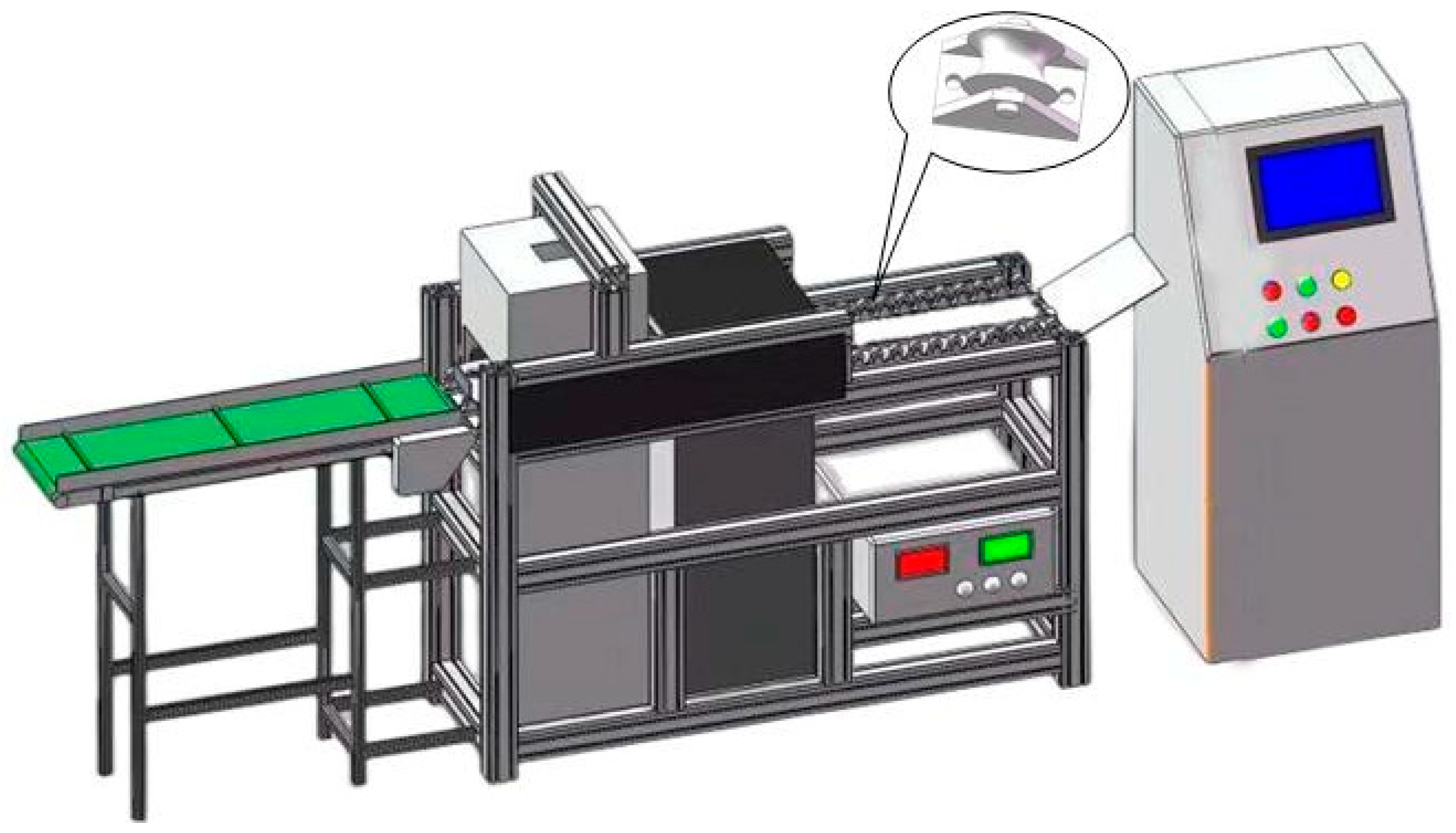
2.1. X-Ray Imaging Detection System

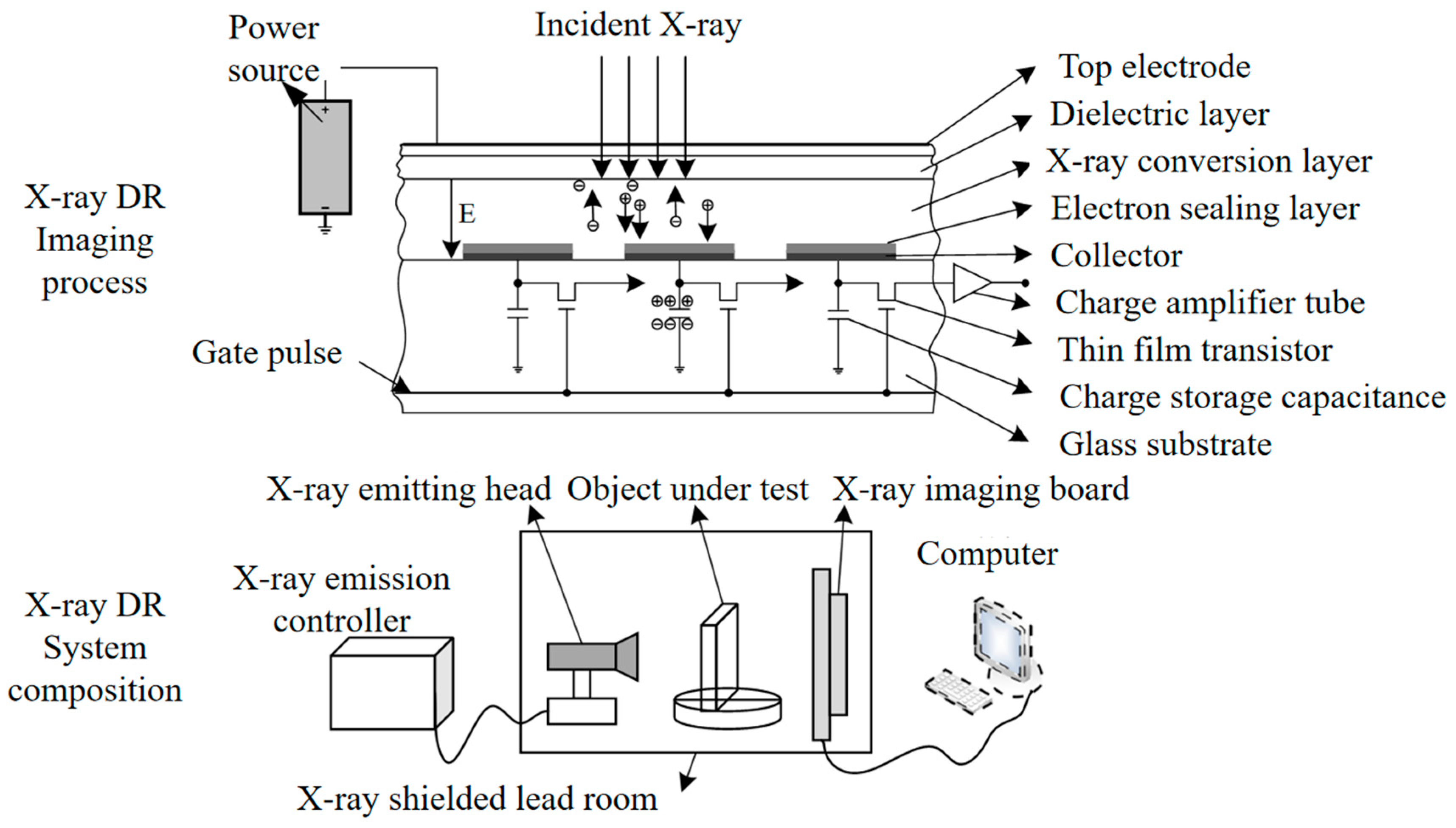
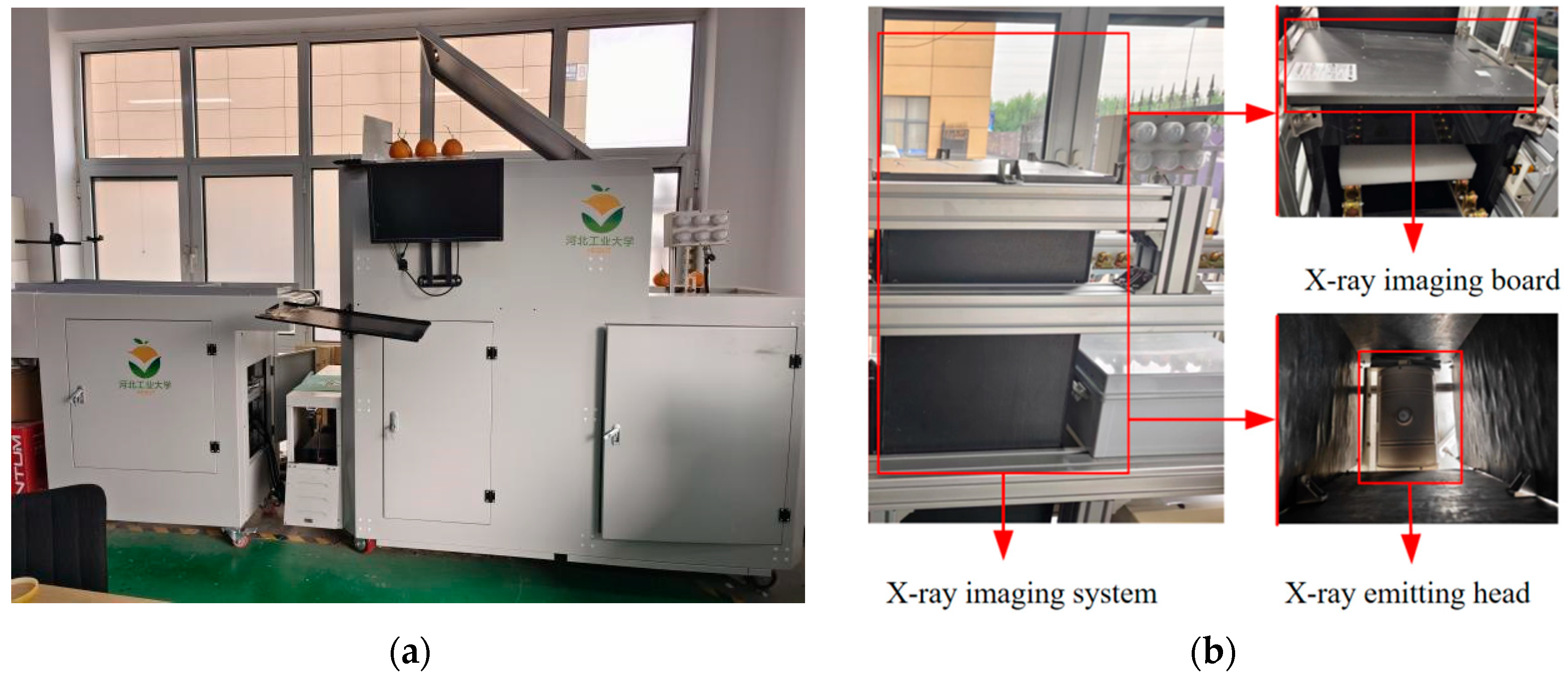
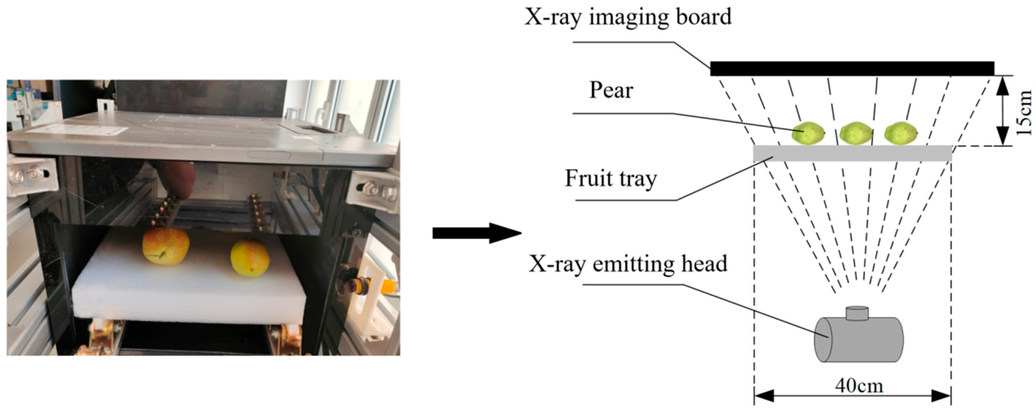
X-ray DR (Direct Radiography) technology uses photoconductive materials for imaging. When X-rays are applied to photoconductive materials, electron-hole pairs are generated. Under the influence of an external electric field, the electron-hole pairs move in opposite directions, creating a current. The magnitude of the current is directly proportional to the number of incident X-ray photons. Thin-film transistors integrate the current into charges for storage. As a result, each thin-film transistor becomes a pixel. Under the action of a field-effect transistor within the pixel, when the electric signal in the pixel unit is read, the charges inside the pixel unit are transferred to the external circuit for release. The read electric signal is amplified and synchronized to be converted into a digital signal, as shown in Figure 1. X-ray DR imaging provides high resolution, can directly output X-ray images, and offers high work efficiency, enabling online detection. For detecting the internal quality of pears, X-ray DR technology is employed.

Using the strong penetrating ability of X-rays, internal defects in pears can be detected. When incident X-rays penetrate the interior of the object, some of the X-ray photons can pass through the object without interacting with it, while others are absorbed by the object, with their energy being absorbed by the object’s electrons, or scattered. The initial energy of the X-ray photons affects their ability to penetrate the object. The initial energy of the X-ray photons can be calculated using the Planck equation:

$$E={\displaystyle \frac{hc}{\lambda }}$$

(1)

where $E$ is the initial energy of the X-ray photons, $h$ is Planck’s constant, $c$ is the speed of light, and $\lambda$ is the wavelength. The shorter the wavelength, the greater the photon energy, and the stronger the penetration ability. X-rays, in particular, have a relatively short wavelength, granting them strong penetration capability. Meanwhile, the density of the object also affects the ability of X-rays to penetrate. The denser the object, the more X-rays it absorbs, and the less it allows penetration. The intensity of monochromatic X-ray transmission through an object follows the formula:

$$I=I_0{e}^{-\mu z}$$

(2)

where $I$ is the transmitted intensity of the X-ray after penetrating the object, $I_0$ is the initial transmitted intensity of the X-ray, $\mu$ represents the attenuation coefficient, which is related to the density of the object, and $z$ denotes the path length of the X-ray through the object.

Since the density of the internal defect areas of the object differs from that of the normal parts, the absorption of X-rays also differs, causing a change in the intensity of the X-rays after passing through the object. This change is captured by the X-ray flat panel detector and is ultimately displayed as an image with varying grayscale distribution. The areas with higher density in the object will have lower grayscale values on the corresponding regions of the image, appearing darker to the human eye.

X-ray imaging is a non-destructive testing method that does not alter the chemical composition or nutritional content of fruits, unlike traditional physical and chemical testing methods. By measuring the internal density variations in the fruit, X-ray imaging effectively detects internal defects without affecting its appearance, hardness, sugar content, or other chemical parameters. When using X-rays to detect internal defects in pears, the density of the defect areas differs from that of the normal tissues, leading to variations in X-ray absorption, which are reflected in the resulting image. However, since the internal defects, core, stem, and calyx parts of the pear may be confused in the 2D X-ray image, misjudgments may occur during quality detection. Deep learning technology lays the foundation for high-accuracy detection.

2.2. Internal Quality Detection Evaluation Indicators of Pears

When performing internal quality detection of pears using X-ray imaging technology, the X-ray images of the pears can clearly reflect internal defects. Since the grayscale variations in the regions corresponding to the fruit stem, calyx, and core in the X-ray image are similar to those in the defect areas, traditional machine learning methods often perform poorly when using X-ray images for non-destructive internal defect detection in pears. This section will focus on the X-ray imaging detection system and the application of deep learning in detecting internal defects in pears using X-ray images.

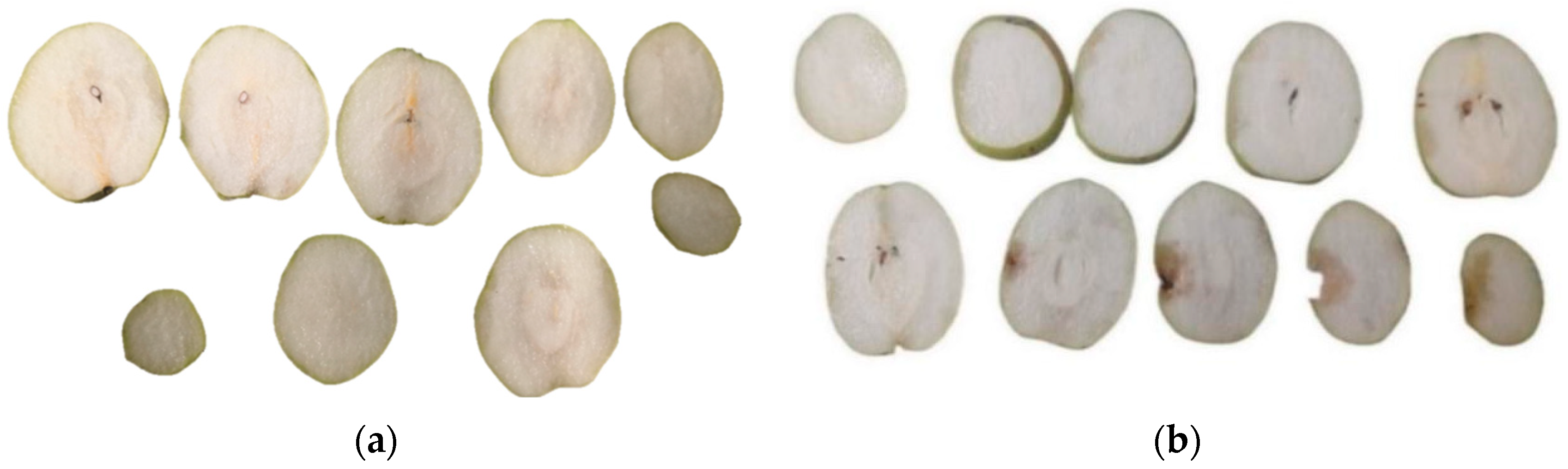
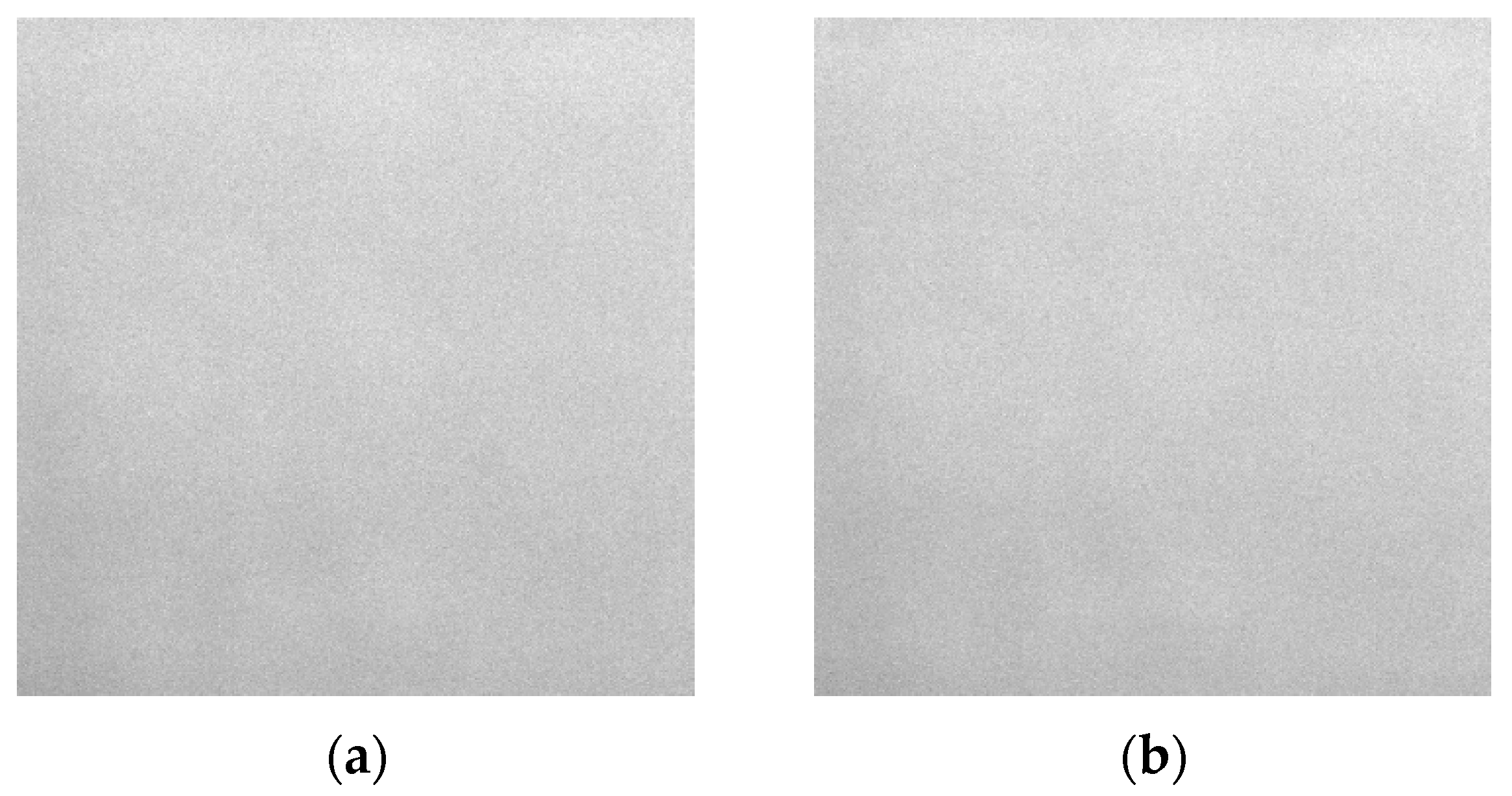
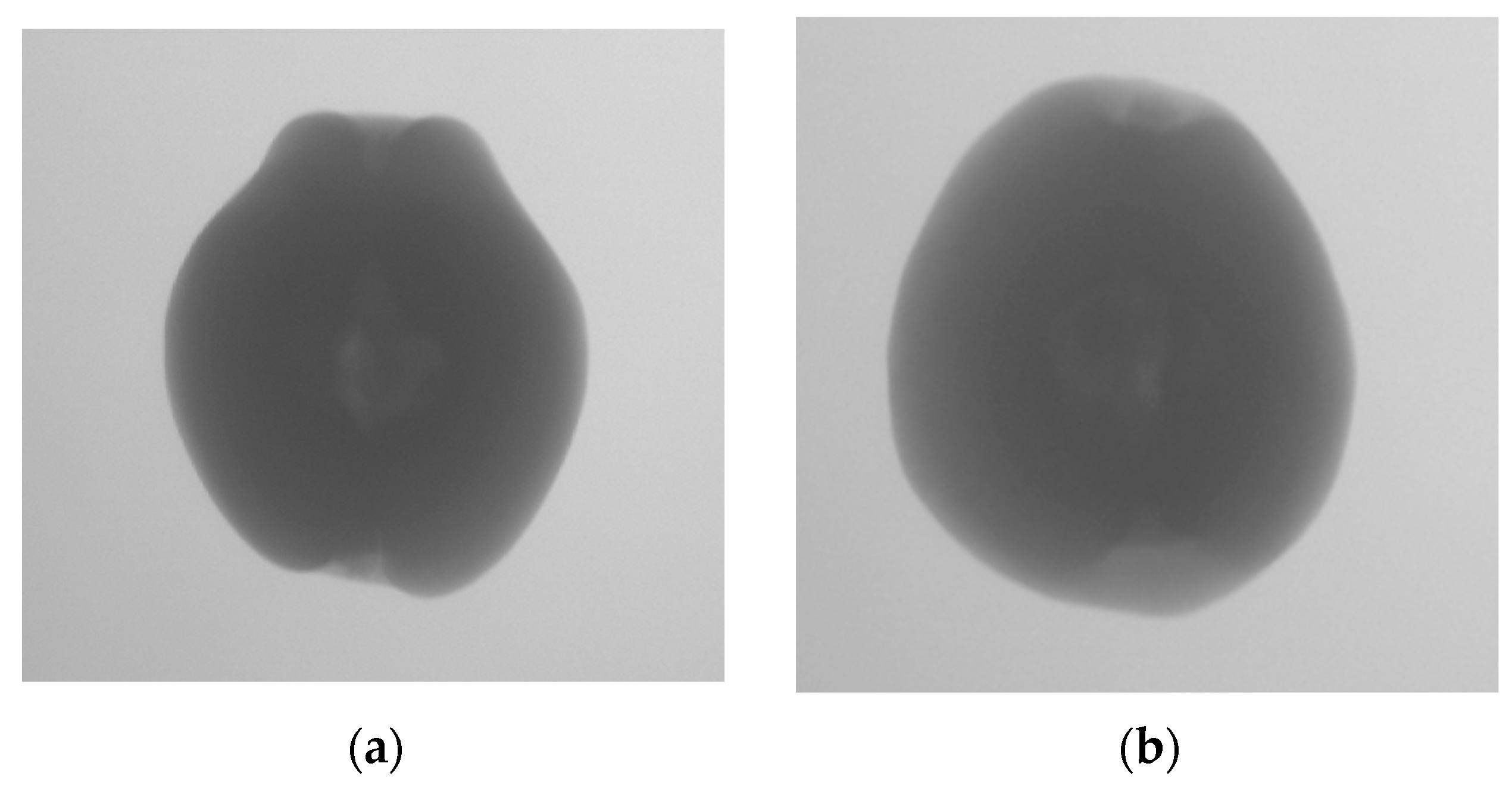
The evaluation of the internal quality of pears is still conducted through manual experiments. First, pears are subjected to X-ray imaging to obtain X-ray images that reflect internal defects. Then, the pears are sliced multiple times after X-ray imaging, and the internal defect information is observed. The internal quality of the pears is evaluated based on this observation, and the X-ray images are annotated accordingly. The annotations are divided into two categories: those with internal defects and those without internal defects, as shown in Figure 2.

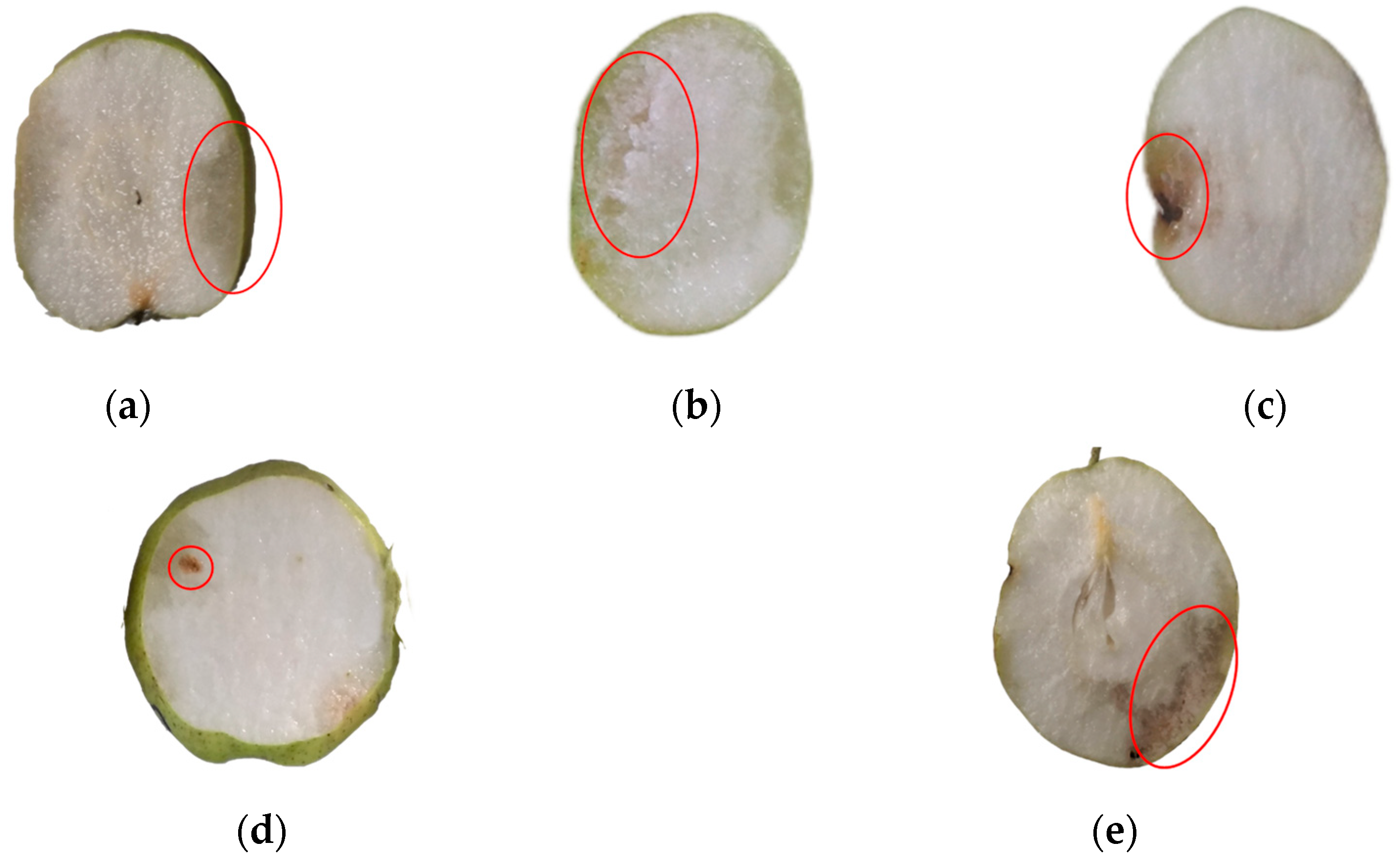
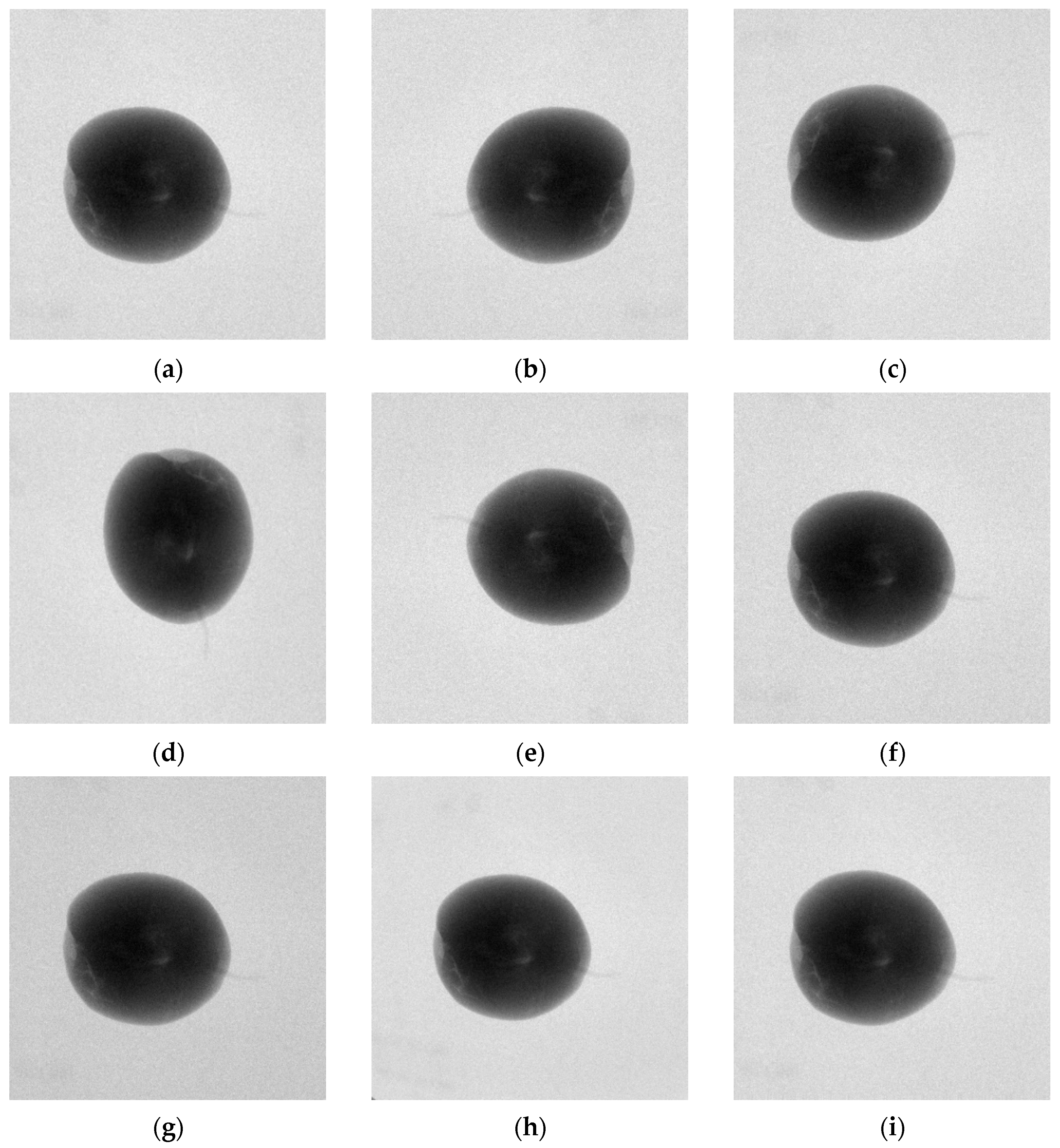
The common internal defects in pear samples discussed in this paper include bruises, russeting, insect infestations, corking, internal rot, etc., as shown in Figure 3. Different types of internal defects in pears can cause changes in the grayscale distribution in the pear’s X-ray image.

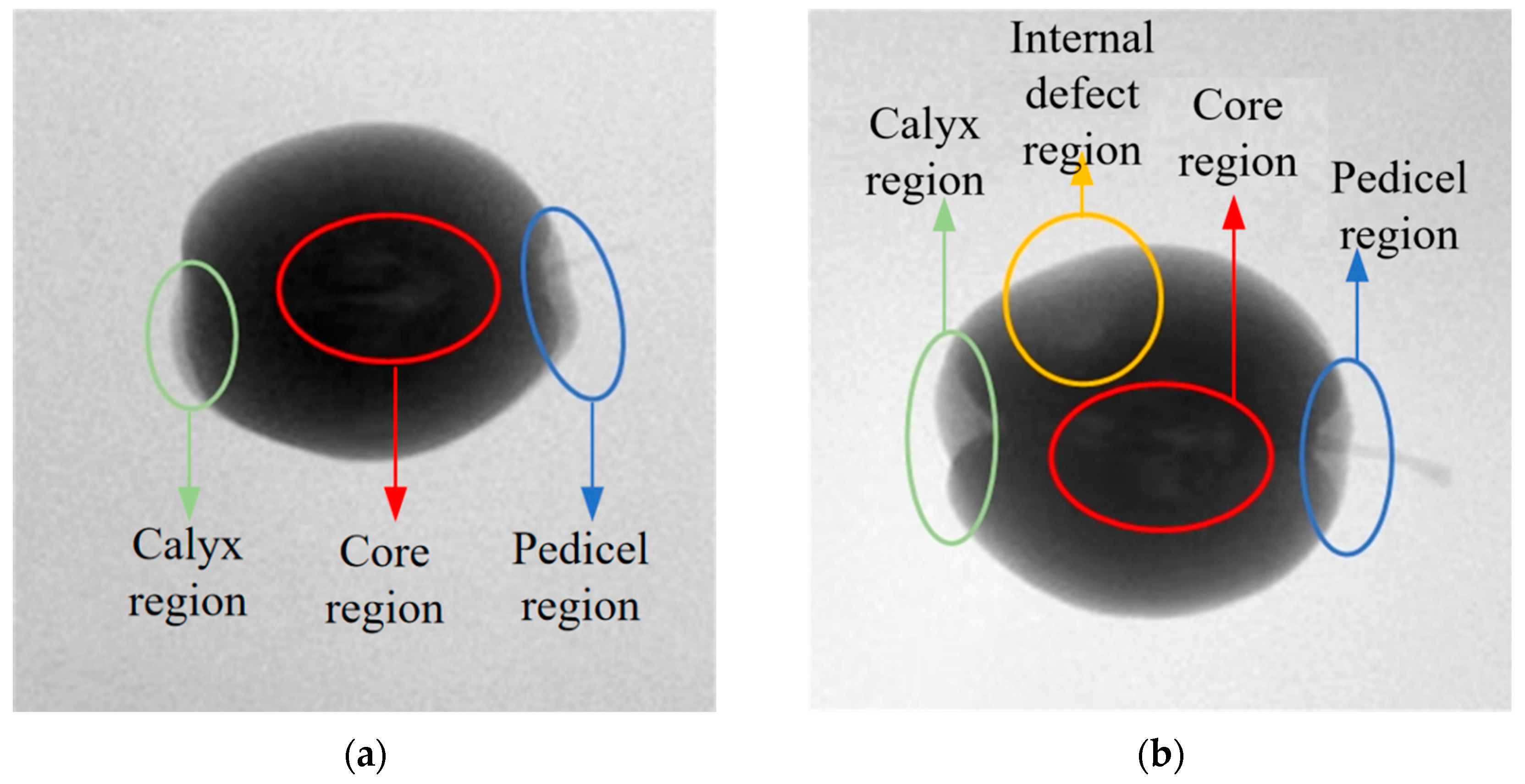
After performing X-ray imaging on the pears, X-ray images are obtained. Figure 4 shows the X-ray images of pears with no internal defects and pears with internal defects. The red circle marks the core region, the green circle marks the calyx region, the blue circle marks the stem region, and the yellow circle marks the internal defect region. It can be observed that there are grayscale value differences between the defective tissue inside the pear and the surrounding healthy tissue in the corresponding X-ray image. Meanwhile, similar grayscale value differences are also present in the X-ray image regions corresponding to the pear’s stem, calyx, and core. This causes interference when judging the internal quality of the pear based on its X-ray image. However, the regions of the pear’s stem, calyx, and core are relatively fixed in distribution compared to the internal defect regions. Based on this observation, we construct a probabilistic spatial prior map, which reflects the likelihood of these structural regions occurring in normalized image coordinates. For instance, the core generally appears near the center of the image, while the stem and calyx are distributed at the top and bottom ends, respectively.

During the inference phase, the spatial prior map is employed to modulate the classifier’s response. When a suspected defect region overlaps with a high-probability structural zone, the classifier applies a confidence suppression mechanism, such as threshold elevation or Gaussian attenuation, to reduce false positives. This allows the model to diminish spurious activations originating from non-defective anatomical features. Moreover, this prior knowledge can be fused with intermediate feature maps from the deep network, serving as a structural guidance signal during training. It encourages the model to focus on truly anomalous regions while suppressing attention to known non-defect areas. As a result, the approach significantly improves the classifier’s robustness, particularly under challenging conditions such as low contrast or background interference, and effectively reduces the overall false detection rate.

2.3. Artificial Feature Classifier and DCNN Classifier

The combination of an artificial feature classifier and a DCNN (Deep Convolutional Neural Network) classifier may promote the improvement of the detection accuracy for internal quality of pears. This paper considers combining the artificial feature classifier and the DCNN classifier under multi-criteria decision theory to enhance the detection accuracy.

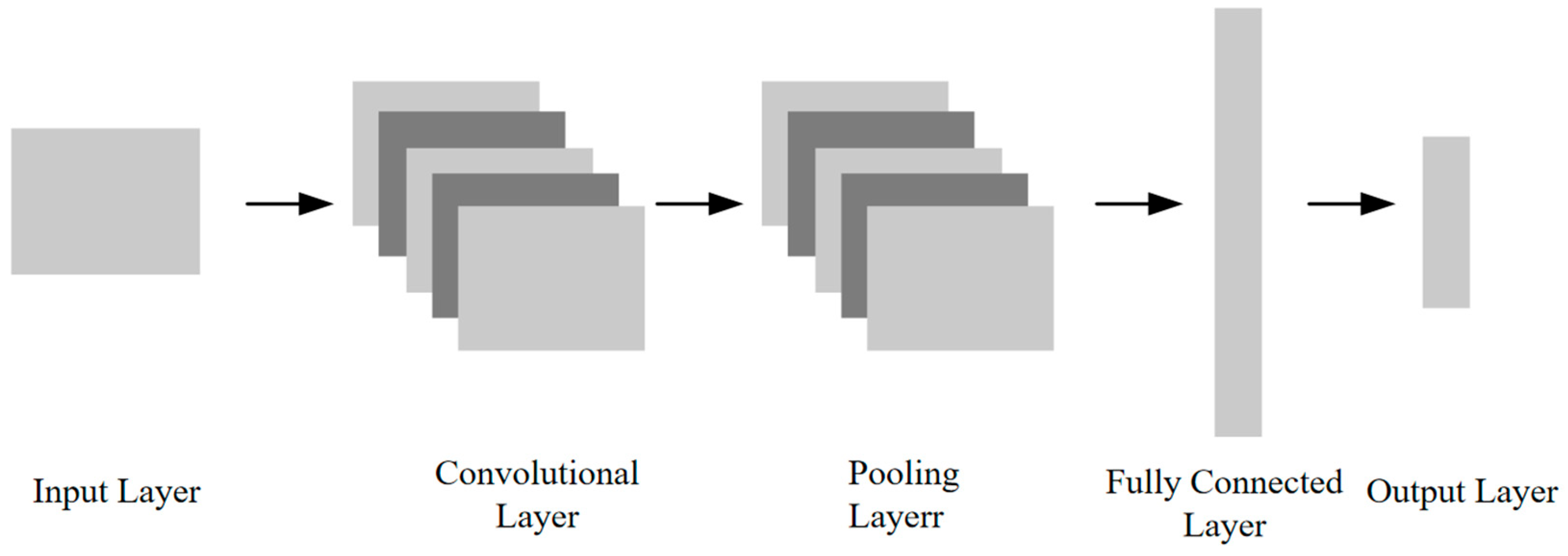
A DCNN is a widely used architecture for object classification, leveraging operations such as feature mapping, weight sharing, local connectivity, and pooling. Typically, a DCNN consists of an input layer, multiple convolutional layers, pooling layers, fully connected layers, and an output layer, as illustrated in Figure 5.

The input layer receives the sample image and feeds it into the network in the form of a tensor. The output layer produces the corresponding category label.

The convolutional layer enables DCNNs to effectively learn representative features by applying fixed-size filters across the input image to capture local spatial patterns. Varying kernel sizes allow for multiscale feature extraction. With a defined stride (S) and padding (P), the filter slides over the input, aggregating local information into a feature map that feeds into the next layer. For square inputs and kernels, the output feature map size is given by

$$A={\displaystyle \frac{W-F+2P}{S}}+1$$

(3)

where $A$ represents the number of pixels along each edge of the square output feature map after the convolution operation, $W$ denotes the size (width or height) of the input feature map, $F$ is the size of the convolutional kernel, $S$ is the stride with which the kernel slides across the input, and $P$ is the number of zero-padding pixels added to the input along each border. When the result of the calculation is not an integer, the output size is typically rounded down using the floor function. The formula for computing the output feature map size is given by

$$f\left[x,y\right]\ast g\left[x,y\right]={\int }_{n_1=-\infty }^{\infty }{\int }_{n_2=-\infty }^{\infty }f[n_1,n_2]·g[x-n_1,y-n_2]$$

(4)

where $f\left[x,y\right]$ represents the input image and $g\left[x,y\right]$ denotes the convolution kernel. The operation is a two-dimensional discrete convolution, which can be intuitively understood as the kernel sliding across the image. At each spatial position, element-wise multiplication is performed between the overlapping regions of the kernel and the input image, followed by summation to produce a single output value in the corresponding location of the feature map.

The pooling layer, or downsampling layer, reduces the spatial dimensions of feature maps to lower computational complexity while retaining key features. Unlike convolutional layers that learn spatial hierarchies, pooling emphasizes feature presence over exact location, enhancing translational invariance. Common types include max pooling, which selects the highest value in a region, and average pooling, which computes the mean.

The fully connected (FC) layer follows the convolutional and pooling stages. Flattened feature maps are passed through one or more FC layers, where each neuron connects to all previous activations, enabling high-level abstraction and classification. The final layer typically employs a Softmax function to convert raw scores into normalized probabilities summing to one, defined as

$$P\left(x_i\right)={\displaystyle \frac{e^{x_i}}{\sum _{k=1}^n{e}^{x_k}}} , i=1,\dots n$$

(5)

where $x_i$ represents $i$-th element in the one-dimensional feature vector, and $P\left(x_i\right)$ denotes its corresponding probability output.

The architecture of a DCNN inherently includes both feature extraction and classification components, allowing it to autonomously learn from image data and extract hierarchical, deep-level features. However, the learned features are often abstract and not easily interpretable by humans, which has led to DCNNs being commonly referred to as “black-box” models. In this study, we exploit the strong feature learning capability of DCNNs to detect internal defects in pears using X-ray imaging, where conventional manual or shallow-feature approaches fall short in capturing subtle structural differences.

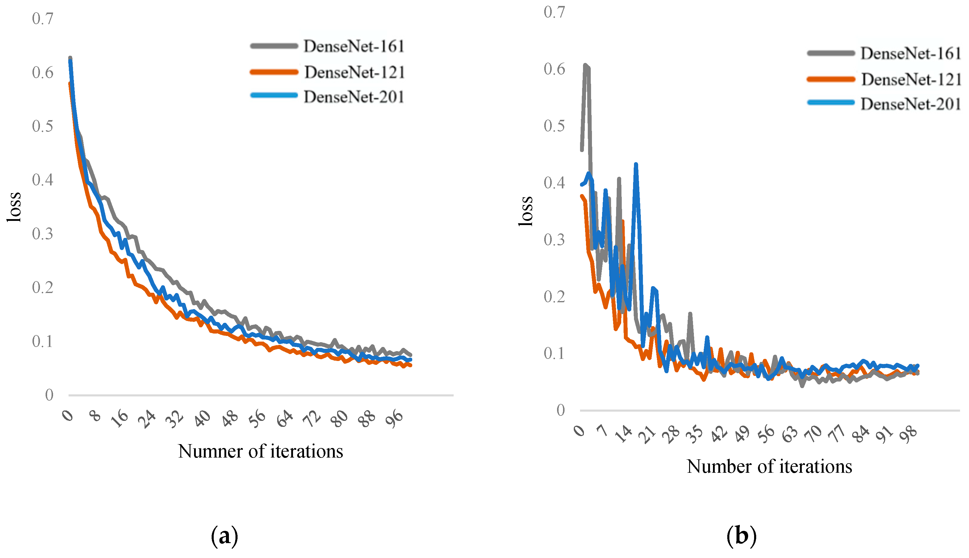
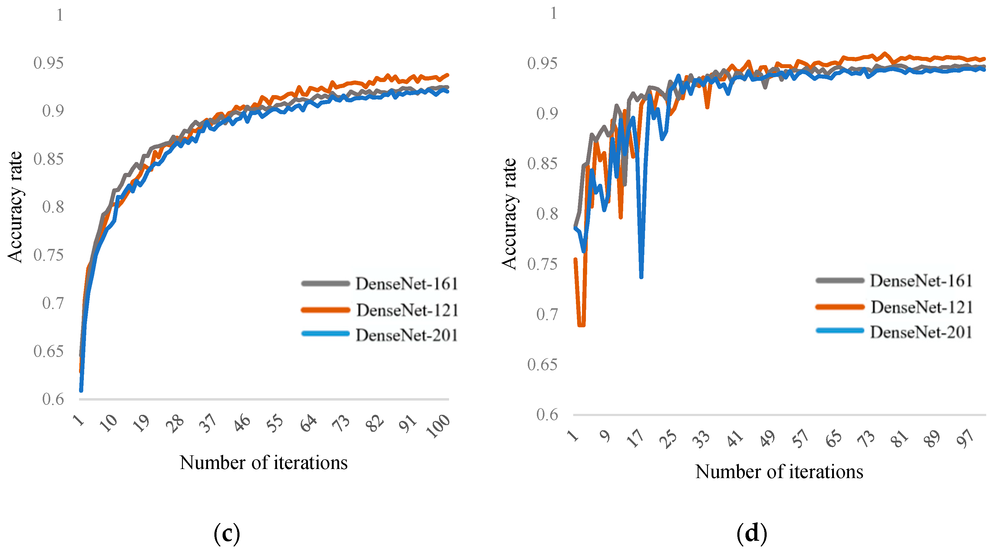
In the process of detecting internal defects in pears using X-ray images, the DCNN channel selects the DenseNet-121 network, which is commonly used in medicine for classifying X-ray images. The network structure is shown in the

Table 1. DenseNet-121 network structure.

Layer Name	Layer Settings	Output Size	Output the Number of Feature Maps
Convolution Layer	$\begin{array}{cc}7\times 7& conv\end{array},stride=2$	112 × 112	64
Pooling Layer	$\begin{array}{cc}3\times 3& max pool\end{array},stride=2$	56 × 56	64
Dense Module(1)	$\left[\begin{array}{cc}1\times 1& conv\\ 3\times 3& conv\end{array}\right]\times 6$	56 × 56	256
Migrating Layer(1)	$\begin{array}{cc}1\times 1& conv\end{array}$	56 × 56	128
	$\begin{array}{cc}2\times 2& average pool\end{array},stride=2$	$28\times 28$	$128$
Dense Module(2)	$\left[\begin{array}{cc}1\times 1& conv\\ 3\times 3& conv\end{array}\right]\times 12$	28 × 28	512
Migrating Layer(2)	$\begin{array}{cc}1\times 1& conv\end{array}$	28 × 28	256
	$\begin{array}{cc}2\times 2& average pool\end{array},stride=2$	14 × 14	256
Dense Module(3)	$\left[\begin{array}{cc}1\times 1& conv\\ 3\times 3& conv\end{array}\right]\times 24$	14 × 14	1024
Migrating Layer(3)	$\begin{array}{cc}1\times 1& conv\end{array}$	14 × 14	512
	$\begin{array}{cc}2\times 2& average pool\end{array},stride=2$	7 × 7	512
Dense Module(4)	$\left[\begin{array}{cc}1\times 1& conv\\ 3\times 3& conv\end{array}\right]\times 16$	7 × 7	1024
Classifier Layer	$\begin{array}{cc}7\times 7& global average pool\end{array}$	1 × 1	—
	$\begin{array}{cc}1000& fully-connected, softmax\end{array}$	—	—

below.

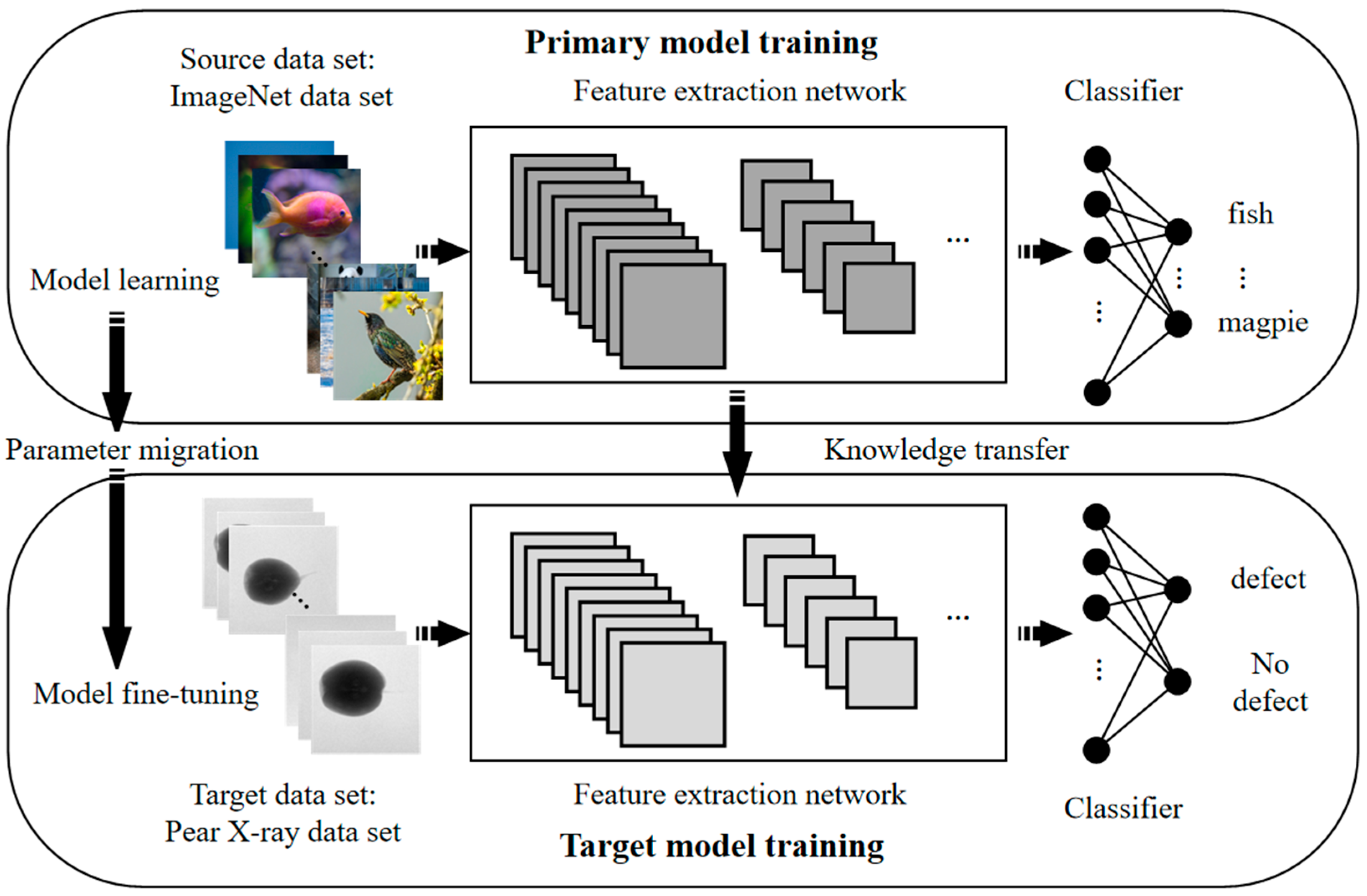
As can be seen from Table 1, the DenseNet-121 network model mainly consists of several Dense blocks and transition blocks. Compared to other DCNN, its advantages lie in reduced parameter quantity and higher computational efficiency. In the final classification, it can utilize both high-level and low-level features, achieving feature reuse and alleviating the problems of gradient vanishing and explosion. Due to the limitations of the dataset, in order to enhance learning efficiency and improve fitting results, although data augmentation was performed, the DCNN still requires large-scale datasets, which are insufficient for this task. Therefore, this paper uses a transfer learning strategy, as shown in Figure 6. The goal of transfer learning is to apply the knowledge learned from a related domain (source domain) to the target domain (target domain). ImageNet is a large-scale dataset used for image classification tasks, containing over 12 million images from 1000 categories. This dataset can be used for pre-training the DenseNet-121 model. The pre-trained model on the ImageNet dataset is then fine-tuned on the pear X-ray dataset for internal quality evaluation based on pear X-ray images.

When training with transfer learning, it is necessary to fine-tune the original model to adapt it to the target classification task. In this paper, the weights of the network before the fully connected layers are frozen, and the output layer of the fully connected layers is modified to suit the internal quality detection task of pears. Then, the model is retrained using pear X-ray images, focusing primarily on training the parameters of the fully connected layers. Once training is completed, the model can be used for detecting internal quality in pears by determining whether internal defects exist based on the X-ray images.

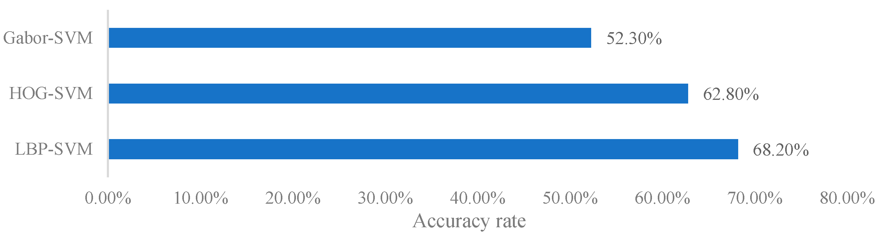
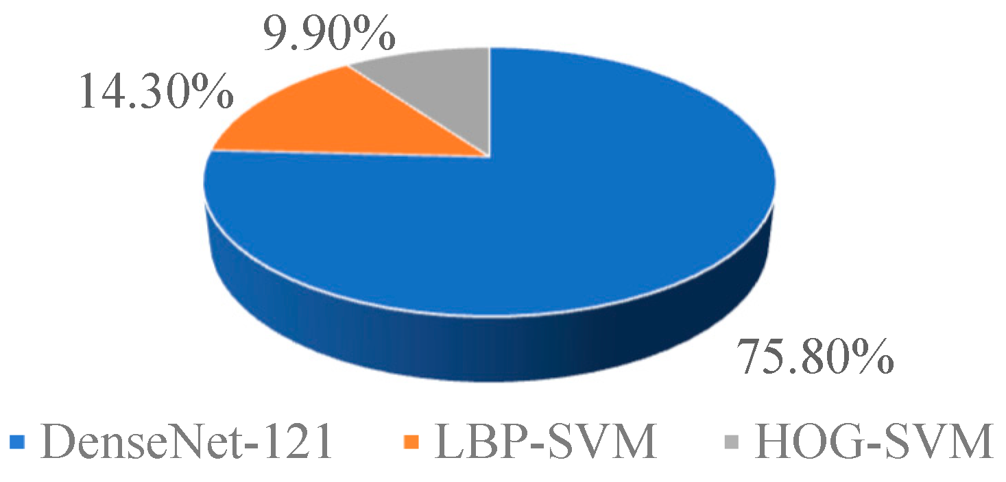
For the artificial feature classifier, commonly used features for X-ray images such as LBP (Local Binary Pattern) and HOG (Histogram of Oriented Gradients) are adopted. In X-ray images of pears, the grayscale variations in the core, stem, and calyx regions are similar to those in defect areas. The use of Local Binary Pattern (LBP) features can effectively prevent confusion between these regions and defect areas, thereby improving detection accuracy. Histogram of Oriented Gradients (HOG) features, on the other hand, are better at capturing edge information in images. When detecting internal grayscale variations in pears, HOG can precisely identify regions associated with internal defects. The integration of these traditional feature extraction methods with deep learning models contributes to enhancing the accuracy of internal quality detection in pears, particularly in the presence of complex image backgrounds and noise interference. Since the detection of internal defects in pears is still a binary classification problem, SVM (Support Vector Machine) is used as the classifier.

LBP is a feature used to describe the local texture of an image. It uses the grayscale value of the specified center pixel $h_c$ as a threshold. The grayscale value of the center pixel $h_c$ is compared with the grayscale values of $P$ neighboring pixels at a distance $R$ from the center pixel, denoted as $(h_0:h_{p-1})$. If the grayscale value of a neighboring pixel is greater than the threshold, it is assigned a value of 1; otherwise, it is assigned a value of 0. Starting from the first pixel $h_0$ at the top left, the values of the $P$ neighboring pixels are read in a clockwise direction to form a binary number. This binary number is then converted into a decimal value, which becomes the LBP value for the center pixel $h_c$. By calculating the LBP value for all pixels in the entire image, the LBP image is obtained. The LBP image is then gridded, and the histogram of the LBP values within each grid is calculated to form the feature vector for that grid. The feature vectors of all grids are concatenated to obtain the final feature vector.

LBP features are grayscale-invariant but not rotation-invariant. To achieve rotation invariance, the $P$ neighboring pixels surrounding the center pixel are rotated with a radius $R$, and a series of initial LBP values are computed. The minimum value from these values is then taken as the LBP value of the center pixel. This process makes the LBP feature rotation-invariant. However, as the number of sampling points increases, the LBP value increases dramatically, which is not favorable for texture recognition. Therefore, dimensionality reduction in the LBP feature is necessary. The number of times the binary LBP value of the center pixel transitions from 0 to 1 or from 1 to 0 is counted. If this number is less than or equal to two, it is classified as an equivalent pattern class; otherwise, it is classified as a mixed pattern class. This reduces the number of possible LBP values for the center pixel significantly, from $2^P$ to $[P\left(P-1\right)+2]$, which greatly reduces the dimensionality of the feature vector. This type of LBP feature is called the LBP equivalent pattern feature, which is one of the features extracted from pear X-ray images in this study.

HOG features can effectively describe the density distribution of local pixel gradient or edge direction in an image. The internal defect regions of pears in X-ray images are presented as variations in grayscale, so HOG features can be used to distinguish whether there are defects inside the pear in X-ray images. The HOG feature vector is generated by concatenating the directional gradient histograms of the local regions in the original image. To suppress noise interference, gamma correction is applied to normalize the color space of the grayscale image. Afterward, the image is processed, and the gradient magnitude and direction of each pixel are calculated. The gradient direction is the object of interest for counting, and the gradient magnitude serves as the weight for the corresponding direction. The grayscale image is gridded, with grid size set as $n_g\times n_g$. The feature vector for each grid is generated by calculating the gradient histogram of the grid. Adjacent grids form a region block, with block size set as $n_b\times n_b$. The number of gradient directions $n_o$, grid size, and block size determine the dimensionality $l$ of the feature vector, with the following formula:

$$l={(floor\left({\displaystyle \frac{224-n_g\times n_b}{n_g}}\right)+1)}^2\times n_b^2\times n_o$$

(6)

By combining DCNN (Deep Convolutional Neural Network) and the artificial feature classifier, the advantages of both methods can be leveraged. DCNN has a stronger ability to learn features and offers advantages in terms of recognition accuracy and generalization ability. Compared to DCNN, the artificial feature classifier still needs improvement in overall recognition accuracy. However, for this study, the artificial feature classifier shows different tendencies in recognizing samples from different categories. The integration of DCNN and the artificial feature classifier under multi-criteria decision theory enhances the recognition ability of the classification model even further. The following section will present experimental verification and result analysis of the internal quality detection method for pears based on multi-criteria decision theory.

2.4. Multi-Criteria Decision Theory

The method of combining multiple classifiers under multi-criteria decision theory includes the construction of an evaluation matrix, normalization and weighting of the evaluation matrix, calculation of the weights of the classifiers in the combination process, and the classification decision process.

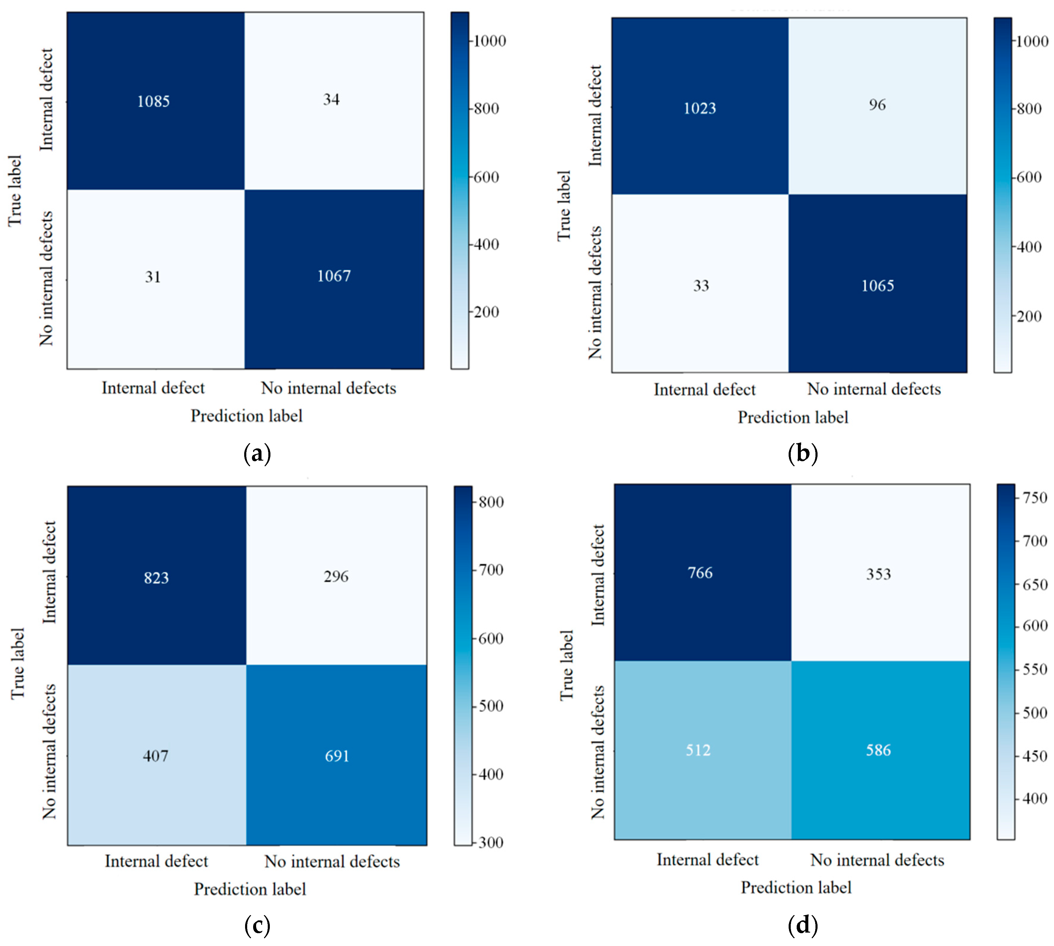
The evaluation matrix is established based on the classification performance metrics of each classifier, including weighted average recall, weighted average precision, weighted average F1 score, accuracy, and Cohen’s Kappa. The above performance metrics are calculated based on the confusion matrix of each classifier. The formulas for calculating the recall, precision, and F1 score for each class are as follows:

$${recall}_i={\displaystyle \frac{{TP}_i}{{TP}_i+{FN}_i}}$$

(7)

$${precision}_i={\displaystyle \frac{{TP}_i}{{TP}_i+{FP}_i}}$$

(8)

$${F1-score}_i={\displaystyle \frac{2\times {precision}_i\times {recall}_i}{{precision}_i+{recall}_i}}$$

(9)

where ${TP}_i$ represents the number of samples that actually belong to category $i$ and are predicted as category $i$, ${FN}_i$ represents the number of samples that actually belong to category $i$ but are not predicted as category $i$, and ${FP}_i$ represents the number of samples that do not belong to class category $i$ but are predicted as category $i$.

The formulas for calculating the weighted average recall, weighted average precision, and weighted average F1 score are as follows:

$$recall={\displaystyle \frac{{\sum }_{i=1}^I{recall}_i}{I}}=1$$

(10)

$$precision={\displaystyle \frac{{\sum }_{i=1}^I{precision}_i}{I}}$$

(11)

$$F1-score={\displaystyle \frac{{\sum }_{i=1}^I{F1-score}_i}{I}}$$

(12)

where $I$ is the number of classes. The formula for calculating accuracy is as follows:

$$accuracy={\displaystyle \frac{{\sum }_{i=1}^I{TP}_i}{A}}$$

(13)

where $A$ is the total number of samples in the validation set. The formula for calculating Cohen’s Kappa is as follows:

$$\mathrm{C}\mathrm{o}\mathrm{h}\mathrm{e}\mathrm{n}\mathrm{’}\mathrm{s} \mathrm{K}\mathrm{a}\mathrm{p}\mathrm{p}\mathrm{a}={\displaystyle \frac{accuracy-p}{1-p}}$$

(14)

where $p$ represents the chance agreement. The formula for calculating it is as follows:

$$p={\displaystyle \frac{{\sum }_{i=1}^H{a}_i{b}_i}{A^2}}$$

(15)

where $a_i$ represents the number of samples in the validation set that actually belong to category $i$, and $b_i$ represents the number of samples in the validation set predicted as category $i$.

The classification performance metrics calculated above are used to construct an evaluation matrix, $Q_{M\times N}={\left(q_{m,n}\right)}_{M\times N}$, where $M=3$, $N=5$, $m=1,\dots ,M$, $n=1,\dots ,N$,$M$ represents the number of classifiers, and$N$represents the number of performance evaluation indicators $C$.$q_{m,n}$ corresponds to the classification performance evaluation metric for each classifier.

The performance evaluation metrics of each classifier are combined with weights ${\alpha }_k$, which are calculated using the following formula:

$${\alpha }_k={\displaystyle \frac{C_k}{\sum _{\mathrm{n}=1}^N{C}_n}},k=1,\dots ,N$$

(16)

where $C_k$ represents the relative importance of each classification performance evaluation metric in the multi-classifier combination. The formula for calculating it is as follows:

$$C_k={\sigma }_k·{\sum }_{j=1}^N\left(1-r_{k,j}\right),j=1,\dots ,N$$

(17)

where ${\sigma }_k$ represents the standard deviation of a classification performance evaluation metric corresponding to all classifiers. The formula for calculating it is as follows:

$${\sigma }_k=\sqrt{{\displaystyle \frac{1}{M}}{\sum }_{m=1}^M{(q_{m,k}-{\overline{q}}_k)}^2}$$

(18)

where $r_{kj}$ represents the elements in the correlation coefficient matrix. The formula for calculating it is as follows:

$$r_{k,j}={\displaystyle \frac{{\sum }_{m=1}^M(q_{m,k}-{\overline{q}}_k)(q_{m,j}-{\overline{q}}_j)}{\sqrt{{\sum }_{m=1}^M{(q_{m,k}-{\overline{q}}_k)}^2·{(q_{m,j}-{\overline{q}}_j)}^2}}}$$

(19)

In Equation (18), ${\overline{q}}_k$ represents the average value of the $k$ classification performance evaluation metric across all classifiers. Similarly, in Equation (19), the meaning is the same.

The evaluation matrix $Q$ is normalized and weighted to obtain $\widehat{Q}$, and the calculation formula is as follows:

$${\widehat{q}}_{m,k}={\displaystyle \frac{{\alpha }_k·q_{m,k}}{\sqrt{{\sum }_{m=1}^M{q}_{m,k}^2}}}$$

(20)

Above is the method for constructing and normalizing the evaluation matrix with weighting. Additionally, the weight ${\omega }_m$ of each classifier in the process of combining multiple classifiers is also evaluated. The calculation formula is as follows:

$${\omega }_m={\displaystyle \frac{d_{m,min}}{d_{m,min}+d_{m,max}}}$$

(21)

where $d_{m,min}$ and $d_{m,max}$ represent the Euclidean distances between the vector ${\overrightarrow{q}}_m$ (Equation (22)), the vector ${\overrightarrow{C}}^{min}$ (Equation (23)), and the vector ${\overrightarrow{C}}^{max}$ (Equation (22)). The calculation formulas for $d_{m,min}$ and $d_{m,max}$ are as follows:

$${\overrightarrow{q}}_m=[{\widehat{q}}_{m,1},\dots ,{\widehat{q}}_{m,n},\dots ,{\widehat{q}}_{m,N}]$$

(22)

$${\overrightarrow{C}}^{min}=[c_1^{min},\dots ,c_n^{min},\dots ,c_N^{min}]$$

(23)

$${\overrightarrow{C}}^{max}=[c_1^{max},\dots ,c_n^{max},\dots ,c_N^{max}]$$

(24)

$$d_{m,min}=\sqrt{{\sum }_{n=1}^N{({\widehat{q}}_{m,n}-c_n^{min})}^2}$$

(25)

$$d_{m,max}=\sqrt{{\sum }_{n=1}^N{({\widehat{q}}_{m,n}-c_n^{max})}^2}$$

(26)

In Formulas (25) and (26), $c_n^{max}$ and $c_n^{min}$ represent the minimum and maximum values of each classification performance evaluation metric across all classifiers, respectively. The calculation formulas for ${\overrightarrow{C}}^{min}$ and ${\overrightarrow{C}}^{max}$ are as follows:

$${\overrightarrow{C}}^{min}=\left\{\min \left({\widehat{q}}_{m,n}|m=1,\dots M\right)|n=1,\dots ,N\right\}=\left\{c_n^{min}\right|n=1,\dots ,N\}$$

(27)

$${\overrightarrow{C}}^{max}=\left\{\max \left({\widehat{q}}_{m,n}|m=1,\dots M\right)|n=1,\dots ,N\right\}=\left\{c_n^{max}\right|n=1,\dots ,N\}$$

(28)

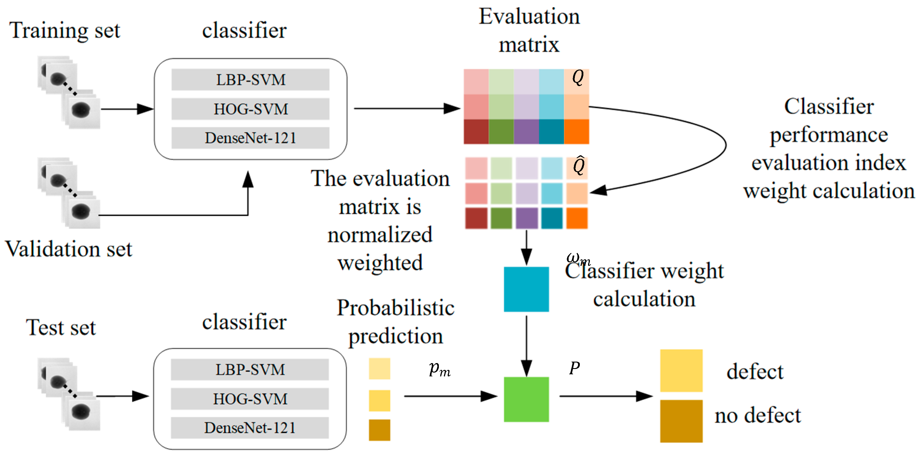
After obtaining the weights of each classifier in the combination process, the next step is to combine the classification decisions from multiple classifiers. As shown in Figure 7, the artificial feature classifier and DCNN classifier are trained using the training set. The validation set is then input into the trained classifiers, and the classification performance evaluation metrics of each classifier are calculated. This completes the establishment and normalization weighting of the evaluation matrix, and the weights of each classifier in the combination process are computed. During the testing phase, the test set is input into each of the trained classifiers to obtain the probability of each sample belonging to the corresponding class. The formula for calculating the probability of each sample in the test set belonging to the corresponding class is as follows:

$$P={\sum }_{m=1}^M{\omega }_m{p}_m$$

(29)

After the above process, the probabilities are converted into classification labels to obtain the final classification result, determining whether there are internal defects in the pear.

3. Results

3.1. X-Ray Imaging System Setup

In this paper, X-ray imaging technology is used for the internal quality detection of pears, and the establishment of the dataset requires an X-ray imaging system. As shown in Figure 8, regarding the X-ray imaging system, the X-ray imaging plate is placed on top of a lead-shielded chamber. The distance between the fruit tray and the X-ray imaging plate is 15 cm, and the X-ray emitter is positioned at the bottom of the X-ray shielded chamber, emitting X-rays from below. The collimator can adjust the coverage of the X-ray to inspect all the fruits. The X-ray imaging system uses DR (Direct Radiography) technology. The relevant parameters of the image acquisition experimental system are shown in

Table 2. Parameters of image acquisition experimental system.

X-ray emitter	Model	SF100BY
	Power supply requirement	Greater than 8 kW (voltage 220 V, current 37 A (instantaneous))
	Launch time range	0–6.3 s (adjustable)
	Transmitting current gear	16, 32, 63, 100 mA
	Transmitting voltage range	40–100 kV
X-ray imaging board	Model	IRay-Venu 1717 X
	Dimension	17 × 17 inches
	Communication Interface/protocol	RJ45 Gigabit Ethernet output
	Resolution ratio	3072 × 3072
	Gray scale	16-bit
Industrial computer	Operating system	Windows 10
	CPU	AMD Ryzen 5 3400G
	Internal memory	8G
	Graphics card	NVIDIA GeForce GTX 1660 (6G)

, and the parameters of the industrial control computer are also explained in the same table.

In addition to the hardware, the pear X-ray image acquisition is performed using the iDetector software (IRay Venu 1717X iDetector A3) on the imaging plate. The X-ray imaging plates provide the necessary interfaces for secondary software development. The pear quality detection and grading software developed after secondary development will be explained in later sections. The subsequent content related to/internal quality detection of pears based on X-ray imaging and pear quality grading will all be developed using Python as the platform.

3.2. Pear X-Ray Image Dataset Construction

3.2.1. Pear X-Ray Image Acquisition

This section describes the acquisition of pear X-ray images using the equipment. Six pears are collected for each image acquisition session. The placement of the pears on the fruit tray is similar to that during the appearance image collection, with the axis of the fruit stem and calyx kept as level as possible. The relative positions of the X-ray imaging plate, the pear, and the X-ray emitter are shown in Figure 9. The pears to be imaged are placed on the fruit tray, and the relevant operating parameters of the equipment are listed in

Table 3. Operating parameters of X-ray imaging equipment.

Parameter Name	Parameter Description
Transmitting voltage	75 kV
Transmitting current gear	63 mA
Launch time	1.6 s
Exposure time	4 s

.

In Figure 9, the pears being imaged are supported by the fruit tray. During X-ray imaging, the X-ray imaging plate is positioned at the top, and the X-ray emitter is positioned at the bottom. When imaging, the X-rays also penetrate the fruit tray, which affects the reflection of the pear’s internal quality in the X-ray image. To reduce the impact on the X-ray imaging quality, foam boards made of EPE material were used as the fruit tray. In the experiment, the X-ray images resulting from the penetration of the fruit tray and the penetration of air were visually indistinguishable to the human eye, which is influenced by the inherent parameters of the X-ray imaging plate, as shown in Figure 10.

3.2.2. Data Augmentation and Dataset Division

Due to the limited number of pear X-ray image samples, data augmentation techniques were employed. Data augmentation increases the dataset size, allowing for more thorough network training and positively contributing to the improvement of detection accuracy. For the pear X-ray images, image segmentation was performed to obtain X-ray images containing only a single pear. Subsequently, image augmentation techniques were applied, including horizontal flipping, vertical flipping, transposition, flipping, random Gamma transformation, random brightness and contrast transformation, optical distortion transformation, and grid distortion transformation. The parameters for image augmentation are shown in

Table 4. Data enhancement method and parameter description of pear X-ray image.

Image Processing Method	Parameter
Horizontal flip	None
Vertical flip	None
Transposition	None
Flip	None
Stochastic Gamma transform	[100, 200]
Random brightness contrast transformation	${limi}_{brightness}=0.1, {limit}_{contrast}=0.1$
Optical distortion transformation	${limit}_{disort}=0.2, {limit}_{shift}=0.2$
Mesh distortion transformation	${limit}_{disort}=0.1, {num}_{steps}=6$

, and the augmented images are shown in Figure 11.

Before image augmentation, the pear X-ray image dataset contained 622 defect-free images and 610 defect images. After image augmentation, there were 11,196 pear images with internal defects and 10,980 pear images without internal defects. Therefore, when using pear X-ray images to classify the presence or absence of internal defects, the sample size for different categories is roughly balanced. The dataset was divided into training, validation, and test sets in a 6:2:2 ratio.

3.3. Experiment and Result Analysis

Before the formal experiment began, to verify whether X-ray imaging would affect the chemical and nutritional composition of pears, we measured the sugar content, acidity, and vitamin C levels before and after imaging. The experimental results showed no significant changes between the pre- and post-imaging measurements, indicating that X-ray imaging does not affect the chemical or nutritional composition of pears.

In the previous sections, we introduced the internal quality detection method for pears based on multi-criteria decision theory. This method aims to improve detection accuracy by combining different classifiers at the decision stage. Traditional classification methods that combine manual feature extraction and machine learning classifiers often do not achieve excellent results for X-ray images. This paper takes further steps by utilizing a common DCNN model for X-ray images in medical applications. Based on the DenseNet-121 classification model, we combined manual feature extraction and machine learning classifiers, merging multiple classifiers. The following sections will present experiments and result analysis based on this method.

Traditional manual features used for image classification include LBP (Local Binary Pattern) features, HOG (Histogram of Oriented Gradients) features, Gabor features, Scale Invariant Feature Transform (SIFT), Speeded Up Robust Features (SURF), and others. In the early stages of this project, the SIFT and SURF were found to be poorly suited for classifying internal defects in pear X-ray images. Figure 12 compares the classification accuracy of internal defects in pears on the validation set of pear X-ray images, using LBP, HOG, and Gabor features combined with SVM. To reduce the feature dimensionality, we used a grid number of 4, and the histogram bin length was set to 12. To retain feature details while reducing feature dimensionality, we set the number of gradient directions to 9 when extracting the HOG features from pear X-ray images. The grid size was set to 8 × 8, and the number of grids in each region block was set to 4. The pear X-ray images were processed with these settings for HOG feature extraction.

From Figure 12, it can be observed that the classification performance of the Gabor feature classifier is only close to random guessing. Although the LBP and HOG feature classifiers perform better than the Gabor classifier, they still fall short of achieving a higher classification accuracy. This suggests that traditional manual feature extraction combined with machine learning classifiers has limited feasibility for classifying the presence or absence of internal defects in pear X-ray images.

For classification using DCNN on pear X-ray images, this study chose the DenseNet-121 network model and compared it with DenseNet-161 and DenseNet-201. The relationship between the loss, accuracy, and the number of iterations for these three DCNN models on the training and validation sets is shown in Figure 13.

From Figure 13, it can be seen that the DenseNet-121 network model converges with fewer iterations during training and quickly reaches a stable minimum for the loss error. In terms of detection accuracy, DenseNet-121 outperforms DenseNet-161 and DenseNet-201 in both the training and validation sets. However, the difference in accuracy is not significant. Considering the large number of parameters in deeper networks, DenseNet-121 is suitable for classifying internal defects in pears.

The machine learning classifiers based on manual features and DenseNet-121 were fused according to the method described in Section 3.2, and the weights of each classifier in the fusion process are shown in Figure 14. At this point, the parameters for the entire fusion model are determined and used for classifying the test set. From Figure 14, it can be seen that DenseNet-121 has the highest fusion weight, which is because the classification performance metrics of DenseNet-121 on the validation set were significantly higher than those of the other two machine learning classifiers.

The fused model was used to classify the test set and compared with the individual application of LBP-SVM, HOG-SVM, and DenseNet-121 classifiers. The confusion matrices of the classification results from the four models are shown in Figure 15. The accuracy, recall, precision, and F1 score for these four classifiers are calculated and presented in

Table 5. Classifier performance indicators of fused model and DenseNet-121, LBP-SVM, HOG-SVM.

	DenseNet-121	LBP-SVM	HOG-SVM	Post-Fusion Model
Accuracy rate	94.2%	68.3%	61.0%	97.1%
95% CI	[92.8, 95.5]	[66.0, 70.4]	[59.2, 63.3]	[96.1, 98.1]
Recall rate	91.4%	73.5%	68.5%	97.0%
95% CI	[89.1, 93.7]	[71.2, 75.7]	[66.0, 70.7]	[96.0, 98.0]
Precision rate	96.9%	66.9%	59.9%	97.2%
95% CI	[95.2, 98.2]	[64.5, 69.3]	[57.1, 62.4]	[96.1, 98.3]
F1 score	94.1%	70.0%	63.9%	97.1%
95% CI	[92.5, 95.8]	[68.1, 71.8]	[61.4, 66.0]	[96.0, 98.1]

. It can be seen that the fused model performs better in classifying the test set, which also demonstrates the effectiveness of the proposed multi-criteria decision-based internal quality classification method for pears.

The reason why the proposed multi-criteria decision-based internal defect grading method effectively improves classification accuracy can be analyzed based on Figure 15 and Table 5. To assess the reliability of the classification metrics, we employed a 1000-iteration bootstrapping method to estimate 95% confidence intervals for each model. The bootstrap approach involved resampling the test set with replacement and recalculating each metric across the resamples. The DenseNet-121 deep learning network performed well in classifying the presence or absence of internal defects in pears, achieving an accuracy of 94.2%. In contrast, the other two machine learning classifiers based on manual features performed poorly. However, by examining the confusion matrices of these classifiers, we can observe the tendencies of LBP-SVM and HOG-SVM for classifying different categories. For negative samples (samples without internal defects), the recall rates of LBP-SVM and HOG-SVM are 62.9% and 53.4%, respectively, which are lower than the recall rates of positive samples (samples with internal defects) at 73.5% and 68.5%. This indicates that the two machine learning classifiers have a stronger ability to distinguish positive samples, which is the reason for the improved detection performance of the fused model.

4. Discussion

4.1. Generalization Ability Evaluation

To evaluate the model’s ability to generalize across different pear varieties and unseen defect types, additional experiments were conducted. Firstly, a variety of pear types with distinct characteristics, such as “Korla Pear”, as shown in Figure 16, were selected for testing. The model performed well across these varieties, successfully detecting internal defects in most cases. However, when tested on pear varieties with subtle structural differences, such as variations in fruit density or skin texture, the model’s performance slightly decreased. Specifically, the accuracy dropped from 97.1% on the original dataset to 94.5% on the new pear varieties. Despite these variations, the model maintained relatively high accuracy for detecting defects, indicating that it could generalize reasonably well to different pear types, but with some limitations when confronted with more nuanced differences.

In addition to testing on multiple pear varieties, the model was also evaluated on unseen defect types. Pear samples with novel defects, such as newly discovered frost damage or atypical diseases, were included in the test set. The model’s performance on these unseen defect types showed a decrease in both accuracy and recall compared to known defect types. This result highlighted a limitation of the model: while it performed excellently on familiar defects, it struggled with recognizing new and rare defects, leading to a higher misclassification rate. This indicates that the model’s ability to generalize to new defect types remains a challenge, underscoring the importance of diversifying the defect types included in the training data. To further assess the model’s generalization ability, cross-validation was employed, where the model was tested on various subsets of the dataset. These subsets included variations in both pear varieties and defect types, providing a comprehensive evaluation of the model’s performance. The cross-validation results revealed that while the model showed strong performance on most subsets, its accuracy fluctuated when tested on pear samples with diverse defect characteristics or from different varieties. This variability suggests that, although the model excels in detecting defects within a specific range of conditions, it faces difficulties when dealing with variations in either the pear variety or defect type.

In conclusion, the evaluation demonstrates that, while the model is robust and effective at detecting common defect types, its generalization ability to handle new pear varieties and unseen defects needs improvement. The model’s performance on novel defects and diverse pear varieties was not as strong, indicating a need for more diverse data to enhance its robustness. Future improvements could involve incorporating a wider variety of pear samples and defect types into the training dataset, along with utilizing advanced techniques such as transfer learning and synthetic data generation. These methods could simulate rare defect scenarios and further boost the model’s generalization capacity, making it more adaptable to real-world applications where diverse products and defect types are inevitable.

4.2. System Latency, Throughput, and Integration Feasibility

The proposed X-ray imaging and multi-classifier fusion method demonstrated a per-sample inference time of approximately 0.85 s, including image preprocessing, DCNN inference, and decision fusion. With a parallelized implementation and optimized batch processing, the system achieves a throughput of ~6 fruits/second, equating to 14,400 fruits/hour, which satisfies typical industrial sorting line speeds (generally 8000–20,000 fruits/hour).

The integration potential into industrial grading lines is promising. The X-ray DR system’s hardware footprint is compact, and the imaging setup (with a 4 s exposure time and 1.6 s launch time) aligns with the conveyor belt-based continuous inspection frameworks, as shown in Figure 17. Moreover, the classification model was embedded into a custom Python-based software platform (Pear internal defect detection software v1) that supports Gigabit Ethernet communication protocols, enabling real-time communication with industrial PLCs and actuators for sorting control.

5. Conclusions

The internal quality of pears is evaluated based on the presence or absence of internal defects. A method based on multi-criteria decision theory for internal quality detection of pears is proposed. This method uses pear X-ray images, extracts LBP and HOG features, and constructs a multi-criteria decision fusion model that includes LBP-SVM, HOG-SVM, and DenseNet-121. The weights of each classifier in the fusion process are determined through the evaluation matrix. Experimental validation of the proposed method is conducted, which includes the construction of the X-ray image dataset (labels determined by pear slicing experiments), validation of the multi-criteria decision fusion model, and internal quality detection experiments for pears. Fusion is performed at the decision layer, combining DCNN with machine learning classifiers based on manual features, resulting in an improvement in detection accuracy. The accuracy of the fused classification model and three individual classifiers (DenseNet-121, LBP-SVM, and HOG-SVM) are 97.1%, 94.2%, 68.3%, and 61.0%, respectively, demonstrating the effectiveness of the proposed method.