Automatic Correction of Labeling Errors Applied to Tomato Detection

Abstract

Accurate labeling is critical for training reliable deep learning models in agricultural applications. However, manual labeling is often error-prone, especially when performed by non-experts, and such errors (modeled as noise) can significantly degrade model performance. This study addresses the problem of correcting labeling errors in object detection datasets without human intervention. We hypothesize that label noise can be reduced by exploiting the feature space representation of the data, enabling automatic refinement through repeated model-based filtering. To test this, we propose a recursive methodology that employs a YOLOv5 detector to iteratively relabel a dataset of Prunaxx and Paipai tomato images captured in greenhouse environments. The correction process involves training the detector, predicting new labels, and replacing existing labelings over multiple iterations. Experimental results show substantial improvements: the mean Average Precision at an IoU threshold of 0.50 (mAP-50) increased from 0.8 to 0.86, the mean Average Precision across IoU thresholds from 0.50 to 0.95 (mAP-50:95) increased from 0.46 to 0.63, and Recall improved from 0.68 to 0.82. These results demonstrate that the model was able to detect more true positives after filtering, while also achieving more accurate bounding box predictions. Although a slight decrease in Precision was observed in later iterations due to false positives, the overall quality of the dataset improved consistently. In conclusion, the proposed filtering method effectively enhances label quality without manual intervention and offers a scalable solution for improving object detection datasets in precision agriculture.

1. Introduction

The technological revolution in agriculture is characterized by increased use of neural networks to optimize crop production [1,2]. Numerous studies have focused on enhancing agricultural yields through the precise detection of weeds, flowers, fruits, and ripe produce using various neural network models [3,4]. The accurate detection of fresh fruits is essential for their classification, reducing labor and the use of chemical products [5,6]. In addition, the growth of the global population and the limited arable land requires the development of controlled agricultural production [5,7]. To meet increasing food demands, farmers are adopting new agricultural technologies; it is essential to produce more crops with lower energy consumption [8,9]. This requires heat-resistant, high-yield, and easy-to-cultivate plant varieties [10,11]. Using available tools and datasets for agriculture will reduce time and labor costs and maximize agricultural productivity [12,13]. Automation in fruit detection not only facilitates automated harvesting operations and fruit development monitoring but also improves field management and optimizes plant quality [14].

Accurate tomato detection is a critical challenge in precision agriculture and agriculture automation. Advances in deep learning have shown promise in this area, enabling highly accurate identification and classification of tomatoes in images. However, this approach faces significant challenges related to the need for more annotated data and difficulties in manual labeling.

Currently, there are two fundamental approaches to object detection algorithms: those based on a single step and those based on two steps. Some examples of two-step algorithms can be found in [15], which presents a method for the accurate and fast detection of ripe tomatoes in plants. This method combines deep learning (F-RCNN) with contour detection (using fuzzy techniques and HSV color space), which efficiently separates target tomatoes from adjacent tomatoes, thus improving detection accuracy. Another interesting work is [16], which presents a paper detailing the development of a detector using the Mask-RCNN algorithm to identify tomatoes in greenhouse images. The results obtained show accurate detection, comparable and even superior to previous works, even under laboratory conditions or with higher-resolution images. In addition, the algorithm can capture the depth of objects, which is crucial for background removal, by taking advantage of a RealSense RGB-D camera as a sensor. On the other hand, in [17], the authors introduce a system based on Mask-RCNN and image processing for crop mass detection and estimation. They perform a backbone modification using Resnet11 with a pyramidal feature network, resulting in accurate detection and segmentation. Regarding single-step-based algorithms, developments stand out, such as the one presented in [18], in which the authors propose a deep learning-based approach for the detection of cherry tomatoes in greenhouses. They use the single-shot multiple-box detector (SSD), with a backbone modification resulting in two distinct networks: one based on Mobilenet and the other on InceptionV2. Results show that the InceptionV2-based network achieves an average accuracy of 98.85%. Algorithms based on the general purpose object detector YOLO also stand out, such as the one proposed in [19], in which the authors present an improved tomato detection model, YOLO-Tomato, based on YOLOv3. It incorporates a dense architecture for improved accuracy and uses a circular bounding box instead of the traditional rectangular one for more accurate tomato localization. This model outperforms other state-of-the-art detection methods in performance. On the other hand, a study by Zheng et al. [20] introduces the YOLOX-Dense-CT algorithm to detect cherry tomatoes effectively. This method uses DenseNet as the basis for YOLOX, precisely adjusting it for these tomatoes, and uses the CBAM attention mechanism to improve feature fusion, achieving an average Precision of 94.80%. In addition, YOLOX-Dense-CT has fewer parameters than comparable models. One of the latest developments can be seen in [21], where it is proposed to employ the YOLOv7 algorithm, to which a new structure called ReplkDext is added to extend the receptive field. In addition, the head structure is redesigned using FasterNet to achieve a tradeoff between speed and accuracy, and ODConv is incorporated to improve feature extraction. The experiments show a 26.9% increase in mAP-50:90 compared with the original YOLOv7.

The main barrier to the effective development of Deep Learning models for tomato detection is the need for extensive and properly annotated datasets. Manual collection and labeling of tomato images require considerable and costly human effort. Existing datasets are often small and may need to capture a sufficient diversity of environmental conditions, tomato varieties, and maturity stages. In addition, the manual labeling process is prone to error and subjectivity, which can result in nonuniform and biased datasets. Variability in tomato shape, color, and size and the presence of occlusions and complex backgrounds further complicate the manual labeling process.

1.1. Related Work

Several automatic labeling methods have been developed to address the paucity of data and the limitations of manual labeling; several automatic labeling methods have been proposed. These methods use image processing and machine learning techniques to generate labels in a semi-automatic or full-automatic manner. In this context of automatic labeling for fruit detection in agriculture, several techniques have been explored to improve the efficiency of the data labeling process.

Among these techniques are semi-supervised learning, which capitalizes on both labeled and unlabeled data for model training; active learning, which involves the strategic selection of samples for labeling, thus maximizing the information obtained from each label; and transfer learning, whereby knowledge gained from one dataset is transferred to another, reducing the need for exhaustive labeling [22,23]. Some existing applications include the work in [24], which addresses the application of active learning with MaskAL to reduce the annotation effort in Mask R-CNN training on a broccoli dataset with visually similar classes. The main objective is to improve the efficiency of automatic labeling in fruit detection. Using active learning techniques, the authors managed to significantly reduce the workload associated with manual data annotation, resulting in a more efficient and accurate fruit detection process in agricultural settings. In [25], the authors present an automatic labeling approach to overcome the limitations of deep learning in applications with insufficient training data, focusing on fruit detection in pear orchards. The study focuses on developing an automatic labeling system that can generate accurate labels for a limited dataset, thus improving the ability of fruit detection models under sparse data conditions. Reference [26] focuses on the automatic construction of automatically annotated datasets for object detection. The study proposes an innovative approach to automatically generate labels, which facilitates the development of more efficient and accurate fruit detection models. In [27], the authors present an automatic image labeling approach based on an improved nearest-neighbor technique with a semantic label extension model. The study focuses on improving the quality and relevance of automatically generated labels, which contributes to the accuracy of fruit detection models in agriculture. Reference [28] proposes a transformer-based maturity segmentation for tomatoes. The study focuses on developing an effective and accurate method for segmenting tomato ripeness using advanced image processing techniques, which contributes to improving the quality and efficiency of fruit detection in agriculture.

Among the most recent works is that in [29], which proposes an adaptive optimized residual convolutional residual image annotation model with bionic feature selection. The goal is to improve the accuracy and efficiency of automatic labeling in fruit detection in agriculture. The proposed model achieves a significant improvement in the quality of the labels generated, which contributes to the general accuracy of the fruit detection systems.

Although machine learning methods are solving many tasks [30,31], the majority of such works are based on the use of supervised approaches, where a curated dataset is available. However, in many cases, the dataset is corrupted, with issues such as missing labels, incorrect boundaries, or incorrectly assigned classes [32]. To overcome these limitations, further research is imperative in robust and scalable automatic labeling methods and synthetic data generation techniques. Therefore, this work aims to contribute to the construction of new knowledge in the area of automatic labeling to facilitate this arduous task.

1.2. Contribution

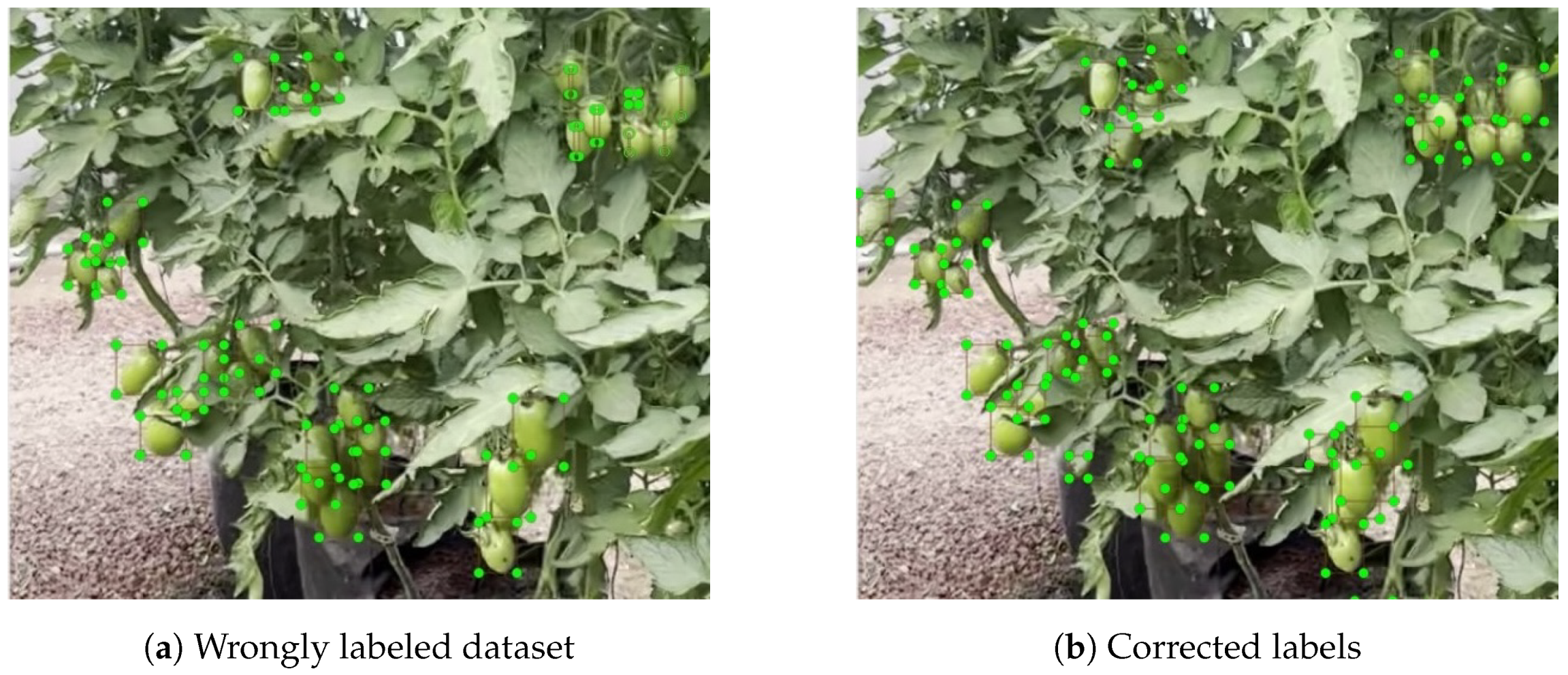
In this paper, we present a case study of tomato detection, where the dataset is composed of pictures taken inside a greenhouse, and the labels are specified as a bounding box with its corresponding object class. The dataset was manually labeled by nonexperts and is not curated. Therefore, it contains errors. These errors are due to displacements in the bounding boxes, which can be seen as perturbations in the image space. Since only a single class is detected in this case, there is no corruption in the class labels. See Figure 1a, where an example picture shows the labels assigned by a non-expert user. If such a dataset is used to train a machine learning model, the model will perform poorly in production because the incorrect labels will affect the predictions. In the literature, it has been shown that the performance of a machine learning model can be improved by introducing human feedback [33], but such interventions require extra effort. Therefore, the problem addressed in this study is to correct labels using only the information within the same dataset.

To address this problem, we propose an iterative refinement of the dataset using a neural network-based predictor that is fine-tuned on the same dataset. Our underlying hypothesis is that errors observed in the image space are averaged in the concept space (also known as the feature space). This averaging happens during the stochastic gradient descent process for mini-batches larger than a single example. To test this hypothesis, we use the YOLO detector [34], which relabels the training and validation datasets after each training session. Each repetition of this process will be called an iteration.

The results show that the dataset is improved to an upper bound as the number of iterations increases. In particular, throughout the iterations, a significant improvement in metrics (mAP-50, mAP-50:90, Precision, and Recall) was observed in the early iterations, reaching a stable point in later iterations, although some false positives increased in the final iterations. Mathematical models were developed to analyze the behavior of the metrics, indicating a generally good fit. The models suggest that as the number of iterations increases, Precision might decrease while other metrics (Recall, mAP-50, and mAP-50:90) improve, reflecting the model’s ability to detect more positive cases under various conditions. However, it is recommended that the number of iterations be limited to no more than four in this study case to avoid an excessive increase in false positives. Then, the presented methodology was applied to correct the labels in a dataset where the labels included perturbations in the bounding boxes. Although the experiments are limited to tomato detection, we believe that this approach is not restricted to this task.

1.3. Paper Organization

The rest of the paper is presented as follows: Section 2 describes the dataset and the methodologies that are applied, and describes the main contribution of the paper: dataset auto-filtering. Next, Section 3 presents the experimentation and result analysis in the study case: tomato detection. Finally, in Section 4, we describe the conclusions and future research directions.

2. Materials and Methods

This section outlines the materials and methodologies employed in this study to ensure reproducibility and transparency. This study was designed to investigate the effectiveness of a novel dataset filtering approach for improving the accuracy of object detection models, specifically in the context of tomato detection in greenhouse environments. Detailed descriptions of the dataset, experimental design, procedures, and analytical techniques are provided below to facilitate replication and validation of the findings.

2.1. Mathematical Notation and Variable Definitions

In this subsection, we formally define the mathematical variables and symbols used throughout this work. These notations are classified by their roles in the dataset, error modeling, neural network learning process, and evaluation metrics.

2.1.1. Notation of Variables Used in YOLO Predictions

The following symbols and terms are used throughout this study to represent the outputs of the YOLO object detection model:

• X: Input image.
• $X_i$: The i-th image in the dataset, where $i=1,\dots ,n$.
• $\widehat{Y}$: Set of all predicted detections for a given image.
• ${\widehat{y}}_i$: Individual predicted detection, where i denotes the index of the detection.
• p: Confidence score indicating the probability that an object exists in the predicted bounding box.
• c: Predicted object class identifier.
• $x,y$: Coordinates of the center of the predicted bounding box (horizontal and vertical, respectively).
• $w,h$: Width and height of the predicted bounding box.

These notations are reused throughout the subsequent sections for model training, label correction, and performance evaluation.

2.1.2. Notation of Variables Used in the Problem Definition

This subsection outlines the following key variables used to formalize the label correction problem:

• $\mathcal{D}$: Original dataset consisting of input images and manually assigned labels.
• L: Set of original ground truth labels corresponding to an image.
• l: Individual label, defined by object class and bounding box parameters.
• e: Perturbation vector modeling labeling errors.
• z: Perturbed label, obtained by applying the perturbation vector to l.
• Z: Set of perturbed labels for a given image.
• $\overline{l}$: Corrected label after applying the filtering procedure.
• $\overline{L}$: Set of corrected labels for an image.
• $\overline{D}$: Corrected dataset obtained after label refinement.
• $D^T$: High-quality test dataset used to evaluate performance.
• ${\Phi }_D,{\Phi }_{\overline{D}}$: Models trained with the original and corrected datasets, respectively.
• $\mathcal{P}(·,·)$: Performance metric used for evaluation (e.g., mAP, Precision).

These variables are essential to the mathematical formulation and analysis of the label correction methodology proposed in this study.

2.1.3. Notation of Variables Used in Hypothesis Explanation

This subsection introduces the following additional variables required to express the theoretical justification of the dataset correction process in terms of concept learning and noise reduction:

• C: True concept representation in the feature space (concept space).
• $T\left(e\right)$: Transformation function that maps labeling noise from the image space into the concept space.
• $\eta$: Learning rate used during the update of neural network weights.
• m: Number of samples in a mini-batch.
• W: Weights of the neural network.

These variables underpin the theoretical assumption that, due to stochastic gradient descent, the model gradually converges toward an averaged concept that mitigates the effects of labeling noise.

2.2. YOLO Predictions

The object detector used in this paper is part of the You Only Look Once (YOLO) family, which employs convolutional neural networks for accurate object detection. These models are recognized for their speed and efficiency, making them ideal for applications that require real-time detection without compromising accuracy. YOLO has been devised in [34]. In [34], YOLO has been improved with subsequent versions, such as YOLOv2 in [35] and YOLOv3 in [36].

In YOLO, object detection is treated as a regression problem instead of a classification problem. This implies that the convolutional neural network (CNN) assigns spatial coordinates to the bounding boxes and computes the probabilities associated with each detected object in a single forward pass.

Let us write a prediction as

$$\widehat{Y}=\mathtt{YOLO}\left(X\right),$$

(1)

where X is an image and $\widehat{Y}$ is a set of predictions,

$$\widehat{Y}=({\widehat{y}}_1,\dots ,{\widehat{y}}_n).$$

(2)

Each prediction is a tuple of six elements,

$${\widehat{y}}_i=(p,c,x,y,w,h),$$

(3)

which represents the confidence of the existence of an object (p), the object’s class (c), the center of the bounding box ($x,y$), and the width and height of the same bounding box ($w,h$).

This approach significantly reduces computational time since image grids perform both detection and recognition. However, it can generate duplicate predictions, a situation addressed by techniques such as non-maximum suppression.

Currently, the original authors of this model have no further modifications to YOLO. However, new versions have continued to be created based on the original model, such as YOLOv4 [37] and YOLOv5 [38] developed by other research groups. The latter was developed by the Ultralytics Working Group, which combines the best of YOLOv3 and YOLOv4. In addition, YOLOv5, a set of open-source object detection models trained on the COCO dataset, will be used in this research. YOLOv5 includes functionalities such as test time enhancement (TTA), model assembly, hyperparameter evolution, and export to ONNX, CoreML, and TFLite, all implemented in the PyTorch 1 framework. This version of YOLO will be used to solve the problem posed in this paper.

2.3. Image Acquisition

The data on tomatoes presented in this paper were collected in a greenhouse in Zempoala, Hidalgo, Mexico, from March to July 2023. The coordinates of the greenhouse are 19°57′22.7″ N, 98°41′40.9″ W, as shown in Figure 2. In this greenhouse, two types of tomatoes were cultivated: Prunaxx and Paipai. The images were captured with a digital camera with a resolution of $1080\times 1920$ pixels. This Full HD resolution is widely adopted in agricultural computer vision tasks and has been shown to be sufficient for detecting small and medium-sized fruits with high accuracy [39,40]. It provides a good balance between image detail and computational efficiency, especially in real-time detection scenarios.

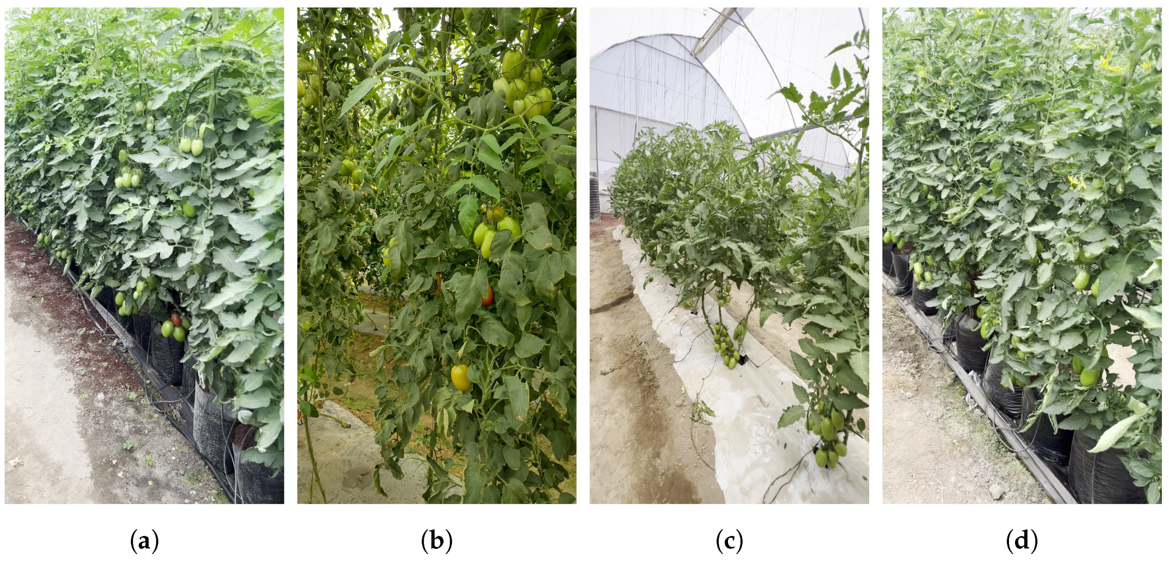
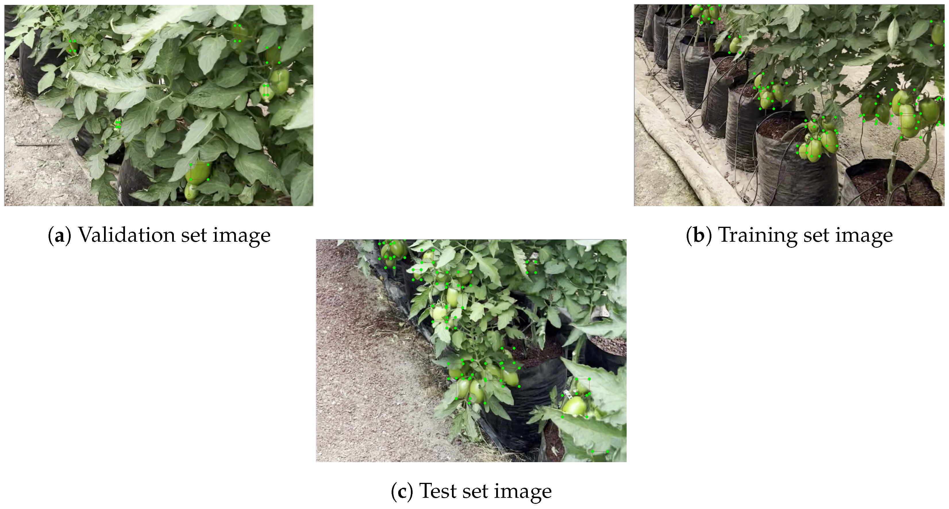
A total of 4391 tomato images were captured at various growth stages, ranging from early fruit development to pre-harvest maturity. This approach ensured a diverse dataset to improve model robustness. The dataset was subsequently divided into a training set, a validation set, and a test set. The dataset was divided as follows: the training set comprised 3538 images (80.6%), the validation set consisted of 752 images (17.1%), and the test set contained 101 images (2.3%). This distribution was designed to ensure sufficient data for training and validation while preserving an independent test set for unbiased evaluation. Figure 3 shows some samples of the dataset in different environments.

In the test set, special attention was paid to labeling the images with utmost precision, as they will be used to validate each experiment. However, in training and validation sets, several images contain labeling errors that can be attributed to human errors. These errors could involve situations such as not defining the entire contour of the tomato, marking only a portion of it, enclosing three tomatoes in a single rectangle, or mistaking a tomato for a part of the leaf. It is important to note that only some tomato labels are correct, as shown in Figure 4.

It is important to note that the training and validation sets were intentionally used in their imperfect state, as the purpose of this work is to evaluate a methodology for automatic correction of labeling errors. These datasets were manually labeled by non-experts and are expected to contain inaccuracies such as partial or misplaced bounding boxes, as shown in Figure 4. Consequently, the initial data used in the auto-filtering method were not assumed to be free of errors. The effectiveness of the correction process was evaluated using a separate, meticulously labeled test set that serves as a reliable benchmark, as described in Section 2.4.

The dataset with labeling errors can be accessed using the following link: https://www.kaggle.com/datasets/gerardoantony/tomate-detection-with-errors (accessed on 6 June 2025).

2.4. Problem Definition

A ground truth dataset can be described as a set of observations, as follows:

$$\mathcal{D}=\{(X_1,L_1)\dots (X_n,L_n)\},$$

(4)

where X is an image and $L=\{l_1,\dots ,l_n\}$ is its corresponding ground truth labels. Note that a label is composed of a set of bounding boxes and classes. In this work, each label is defined by a class and a bounding box, namely,   

$$l=(c,x,y,w,h),$$

(5)

where c is the object class, x is the horizontal center of the object, y is the vertical center of the object, and w and h are the width and height of the bounding box.

Since the labeling is performed manually, it is prone to human errors. To formalize this, let us suppose that the registered label is affected when

$$z=l\oplus e,$$

(6)

where $e=(e_c,e_x,e_y,e_w,e_h)$. This implies that $e_l$ is a label that could or could not be the same as c, while $e_x,e_y,e_w,e_h$ are random variables, zero centered and under the normal distribution. This could be seen as an observation that is perturbed by random errors. Formally, the operation ⊕ is defined as

$$l\oplus e=\left(\begin{array}{c}{e}_c\\ x+e_x\\ y+e_y\\ w+e_w\\ h+e_h\end{array}\right)$$

(7)

From Equation (7), we observe that the ground truth values are perturbed. In the case of the label, it is entirely replaced by the provided value. For the remaining elements, those are perturbed by the random values. Therefore, as in many other tasks, we obtain a perturbed dataset whose errors are introduced by the labelers. When the labelers are experts, we expect that the errors introduced will be close to zero. To formalize, we define a perturbed dataset as

$$D=\{(X_1,Z_1)\dots (X_n,Z_n)\}$$

(8)

Considering Equation (6), we can establish the general problem as estimating the ground truth l from z. Since the perturbation, e is unknown; the real values, l, will remain unknown. However, we expect to compute a better approximation of l. We will call such approximation a corrected label,

$$\overline{l}=(\overline{c},\overline{x},\overline{y},\overline{w},\overline{h}).$$

(9)

With this estimation, a corrected dataset can be built, namely,

$$\overline{D}=\{(X_1,{\overline{L}}_1)\dots (X_n,{\overline{L}}_n)\}.$$

(10)

To validate that $\overline{D}$ is a better dataset than D, we can use an indirect way to measure its goodness. For this paper, we propose measuring the precision of the corrected dataset on a given target task that has good ground truth values. Formally, let us suppose a target task provided by a target dataset, $D^T=\{(X_1^T,L_1^T)\dots (X_n^T,L_n^T)\}$. It is a dataset that has suitable labels. In fact, we are using the super index T to specify that the value is used as a test value. Therefore, it will be used as a test set. Therefore, we will consider that a model is well trained if its performance evaluated on $D^T$ is closer to 1 (considering that zero is the worst performance and one the best). Given the previous definitions, we formalize the problem as follows:

To compute a corrected dataset $\overline{D}$, so that

$$\mathcal{P}({\Phi }_{\overline{D}}\left(X^T\right),L^T)>\mathcal{P}({\Phi }_D\left(X^T\right),L^T),$$

(11)

this can be read as to estimate a corrected dataset, $\overline{D}$, so that if a model is trained with it, ${\Phi }_{\overline{D}}$, such trained model will perform better, under the performance metric $\mathcal{P}$, on a target dataset than the same model trained with the raw dataset, ${\Phi }_D$ (manually labeled with errors), on the same test dataset.

2.5. Dataset Auto-Filtering

To compute a corrected dataset, we propose using the same stored labels and refining them. Our main idea is to train a model recursively, meaning we train a model with the current labels and then use the trained model to refine those labels. We hypothesize that when the model is trained, stochastic gradient descent combines all the errors and causes the predictions to be the average of those errors.

The process starts with the manually labeled dataset, identified as $D_0$. Additionally, we have a predictor capable of solving the task. For this paper, we consider the predictor to be an instance of the YOLO predictor [34]. The YOLO predictor with default parameters (weights) is written as $\Phi$. Then, to compute the corrected dataset, we recursively execute the estimation using Algorithm 1 for n iterations. In other words, we used the previous dataset, ${\overline{D}}_{t-1}$, to estimate a new dataset, ${\overline{D}}_t$, n times.

The recursive estimation (Algorithm 1) requires the previous estimated dataset ${\overline{D}}_{t-1}$ and a trainable predictor $\Phi$. The first step is to set the estimation as an empty set, line 1. The predictor is then trained using the previous dataset, line 2. For this study, YOLO is trained using back-propagation and gradient descent to detect tomatoes in the images. Details of the training are provided in Section 3.2.2. The trained model is written as ${\Phi }_{{\overline{D}}_{t-1}}$. Then, the new labels are estimated in lines 3 to 6. Each image of the dataset, x, is passed to the trained predictor, a set of objects is detected, $\widehat{Y}$, and a label accompanies each detection. The new labels are then predicted by updating the previous labels and the detected objects. This update is explained in Section 2.5.1. Finally, the input image, X, is matched with the estimated labels, $\overline{L}$, and they are added to the estimated dataset, line 6.

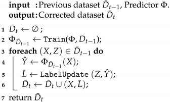
Algorithm 1: Dataset Filtering ($\Phi ,{\overline{D}}_{t-1}$).

The filtering mechanism in Algorithm 1 helps reduce labeling errors by leveraging the model’s internal representation of objects. After each training phase, the YOLO model captures the average concept of the labeled data, which is then used to relabel the dataset. Over multiple iterations, this process reduces inconsistencies in the original annotations by refining bounding box placements, thus minimizing annotation noise and aligning the labels with the model’s learned features.

2.5.1. Label Update

The dataset filtering computes new labels. Therefore, it is necessary to have a rule for carrying out the update of the label. This process is called label update. There are several ways to perform ii: (i) replacement, (ii) averaging, or (iii) weighted averaging.

Full replacement. As a first approach, in this paper, we use full replacement; namely, given an input X, the previous label, Z, is completely replaced by the predicted label, $\overline{Y}$. Formally, the updated labels are computed as

$$\mathtt{LabelUpdate}(Z,\widehat{Y})=\bigcup _{{\widehat{y}}_i\in \widehat{Y}}\left(\begin{array}{c}{\widehat{y}}_i\left[c\right]\\ {\widehat{y}}_i\left[x\right]\\ {\widehat{y}}_i\left[y\right]\\ {\widehat{y}}_i\left[w\right]\\ {\widehat{y}}_i\left[h\right]\end{array}\right)$$

(12)

Equation (12) formalizes the full replacement approach for label correction. In this method, the previously annotated label Z is entirely substituted by the predicted label $\widehat{Y}$ obtained from the trained detector. This choice ensures that the updated dataset accurately reflects the model’s current understanding, which is derived from training on potentially noisy data. Although this can lead to variations in the number of labeled objects over iterations, as described in Section 3.1, it also enables the model to converge to a cleaner concept representation through repeated refinement progressively. We chose this approach instead of averaging strategies to maximize the impact of learned features in the concept space and minimize reinforcement of original annotation errors.

Equation (12) has the consequence that the number of detected objects varies as the iteration progresses. This could happen because the trained predictor could detect more or fewer objects with respect to the old labels. This issue is commented on in the experiments section.

2.5.2. Hypothesis Explanation

From stochastic filtering theory [41], we know that every measurement is inaccurate but relatively close to the real value. As the reading deviates from the true value, its uncertainty increases. This effect can be observed in Equation (7), which can be rewritten as follows:

$$z=\mathrm{x}+e,$$

(13)

where $\mathrm{x}$ is the true value and e is a random variable with an assumed distribution. Such perturbations, e, occur in the image space, meaning that incorrect labels are applied by humans, introducing errors in terms of pixels. However, when training a model, these errors are translated into the feature space, consequently leading to incorrect concepts. Thus, we can write that a concept will be affected by an incorrect label, as follows:

$$\mathcal{Z}=\mathcal{C}+\mathcal{T}\left(e\right)$$

(14)

This means that the learned concept, $\mathcal{Z}$, is the true concept, $\mathcal{C}$, perturbed by the error mapped to the concept space. $\mathcal{T}\left(e\right)$ is a theoretical function that transforms pixel errors to concept space.

For a single example, we believe that there is no way to improve the learned concept; however, for multiple examples, the learned concept is averaged across all readings. This is encapsulated in stochastic gradient descent theory [42], where network weights are updated using the average loss gradient.

$$W\leftarrow W+{\displaystyle \frac{\eta }{m}}\mathcal{L}(\Phi (W,X),Z),$$

(15)

where W represents the weights, $\eta$ is the learning rate, and m is the number of examples. Notice that $\mathcal{L}(\Phi (W,X),Z)$ compares the predictions with the perturbed readings. Therefore, once the weights are updated, they average the concept.

$$\overline{\mathcal{Z}}=\mathcal{C}+{\displaystyle \frac{1}{m}}\sum _i\mathcal{T}\left(e_i\right)$$

(16)

Our main hypothesis is that, after training, the concept is averaged. Sampling from the averaged concept $\overline{Z}$ corresponds to making predictions using a trained model on an input image, X, i.e.,

$$\mathrm{Sample}\left(\overline{\mathcal{Z}}\right)={\Phi }_{\mathrm{trained}}\left(X\right),$$

(17)

where X is the input image and ${\Phi }_{\mathrm{trained}}$ is the trained YOLO model.

The new samples are anticipated to exceed the original samples. To this end, a meticulously labeled test set is employed, serving as a benchmark to assess the progress of the relabeling process. This process can be repeated with the new samples. However, just as filtering an image reduces noise but can also erase the image if applied excessively [43], repeated concept filtering could diminish the concept. In the following section, we provide positive evidence supporting the validity of this hypothesis.

3. Results and Discussion

A series of iterations was carried out using a progressive relabeling approach, detailed in Section 2.5. Initially, the dataset contained labeling errors, as illustrated in Figure 5a. The training was first performed with the dataset that contains these incorrect labels in both the validation and training sets, as shown in Figure 4. After completing the first training cycle, the training and validation sets were relabeled to retrain the model. Each of these training processes was referred to as an iteration, and a total of seven iterations were carried out. Although a significant improvement was observed in Figure 5h from the first to the second iteration, this improvement stabilized with increasing iterations. In some cases, a slight decrease was observed due to increased false positives in some images. Despite this, the improvement compared with the original dataset was significant in each of the iterations.

A computer equipped with 128 GiB of RAM, an AMD Ryzen 7 5700 G processor with Radeon X16 graphics, an NVIDIA GeForce RTX 3090 graphics card, and the Ubuntu 22.04.3 LTS operating system was used to train the neural networks in each iteration. In these experimental tests, the image dataset obtained from the greenhouse, as mentioned in Section 2.3, was used. To carry out these experiments, YOLOv5 was used with the parameters specified in [44], including a learning rate of $1\times {10}^{-3}$ and a batch size of 16, along with the ADAM optimizer. The neural network was trained for 200 epochs.

3.1. Iterative Filtering Results

Figure 5 illustrates that changes occur from the first iteration, and many tomatoes are fully recognized. This process gradually improves, but in the last three iterations, while some false positives are eliminated, new false positives also emerge. This occurs because relabeling the validation set tends to create some false positives in the training dataset. However, an overall improvement is evident compared with the initial state. 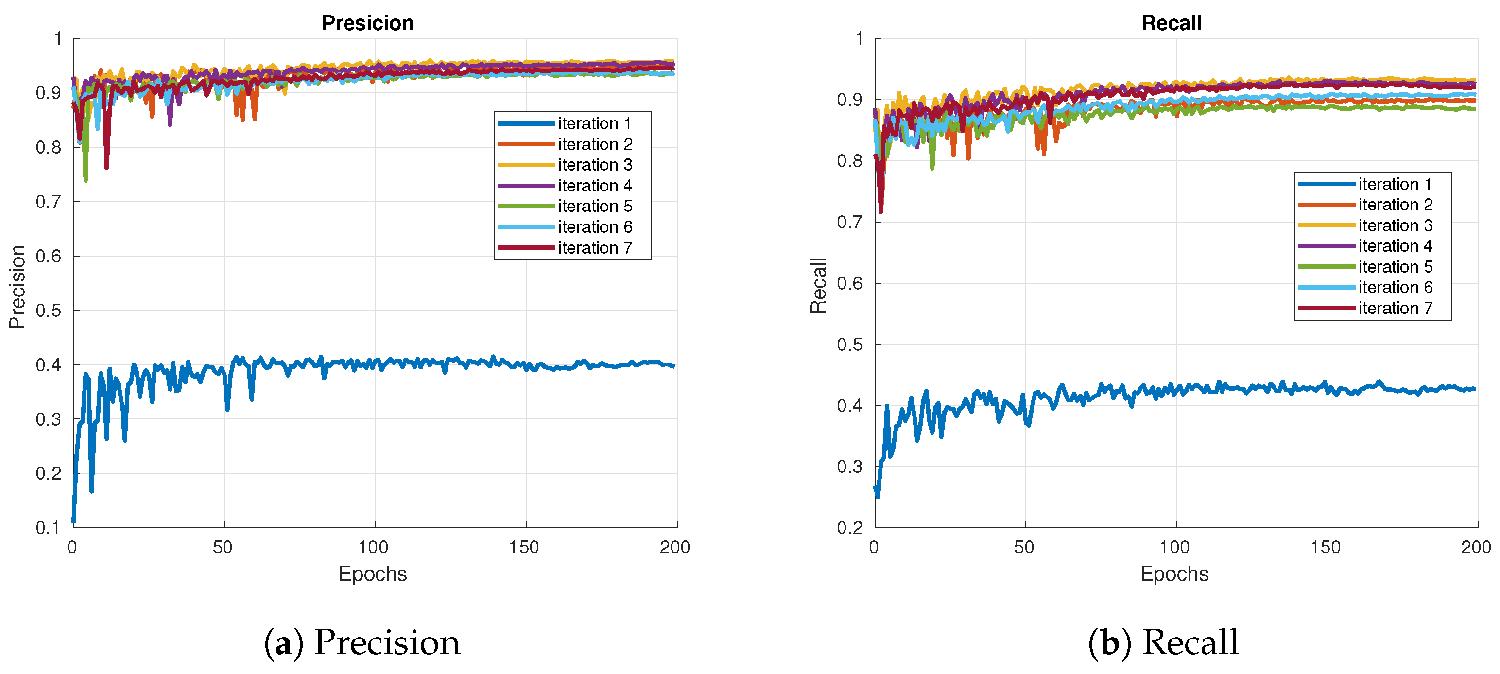Figure 6 displays the losses and metrics obtained during training at each iteration: Training Object Loss, Validation Object Loss, Training Box Loss, Validation Box Loss, Precision Metric, and Recall Metric.

Figure 6a depicts the Precision Metric for each iteration. This metric evaluates the accuracy of bounding boxes in unseen data during training, indicating the percentage of true positives among all predictions made by the model in each iteration. In other words, it measures how many of the predicted objects are actually present in the data. The Recall Metric for each iteration is shown in Figure 6b, indicating the percentage of true positives among all actual instances of objects in the data for each iteration, focusing on the model’s ability to detect all positive cases. In other words, it measures how many of the actual objects are detected by the model.

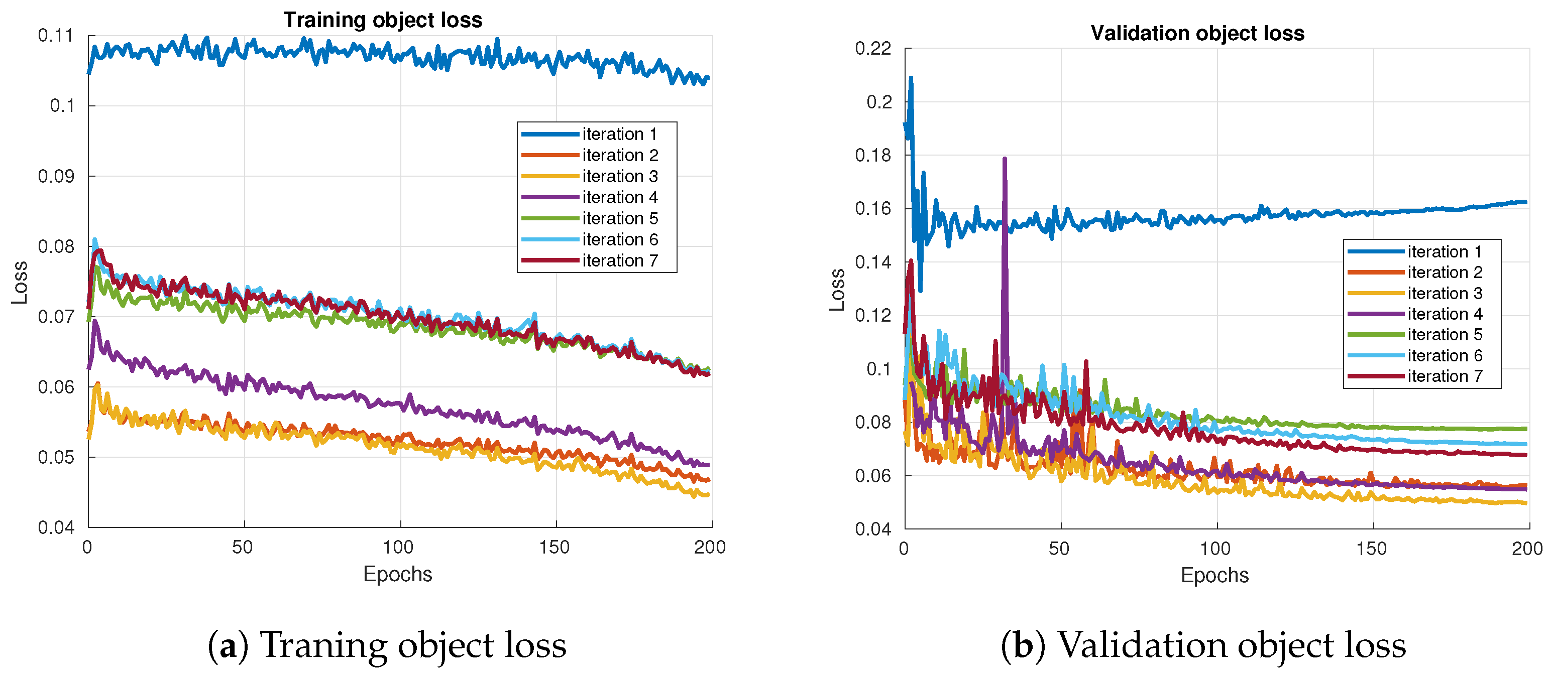
Figure 7a shows the loss of training objects, representing the loss associated with object detection in the training dataset. This graph helps identify the iteration that best predicts the presence of objects during training. Figure 7b illustrates the Validation Object Loss, which refers to the loss associated with object detection in the validation dataset. This metric assesses the model’s generalization capability with data not seen during training.

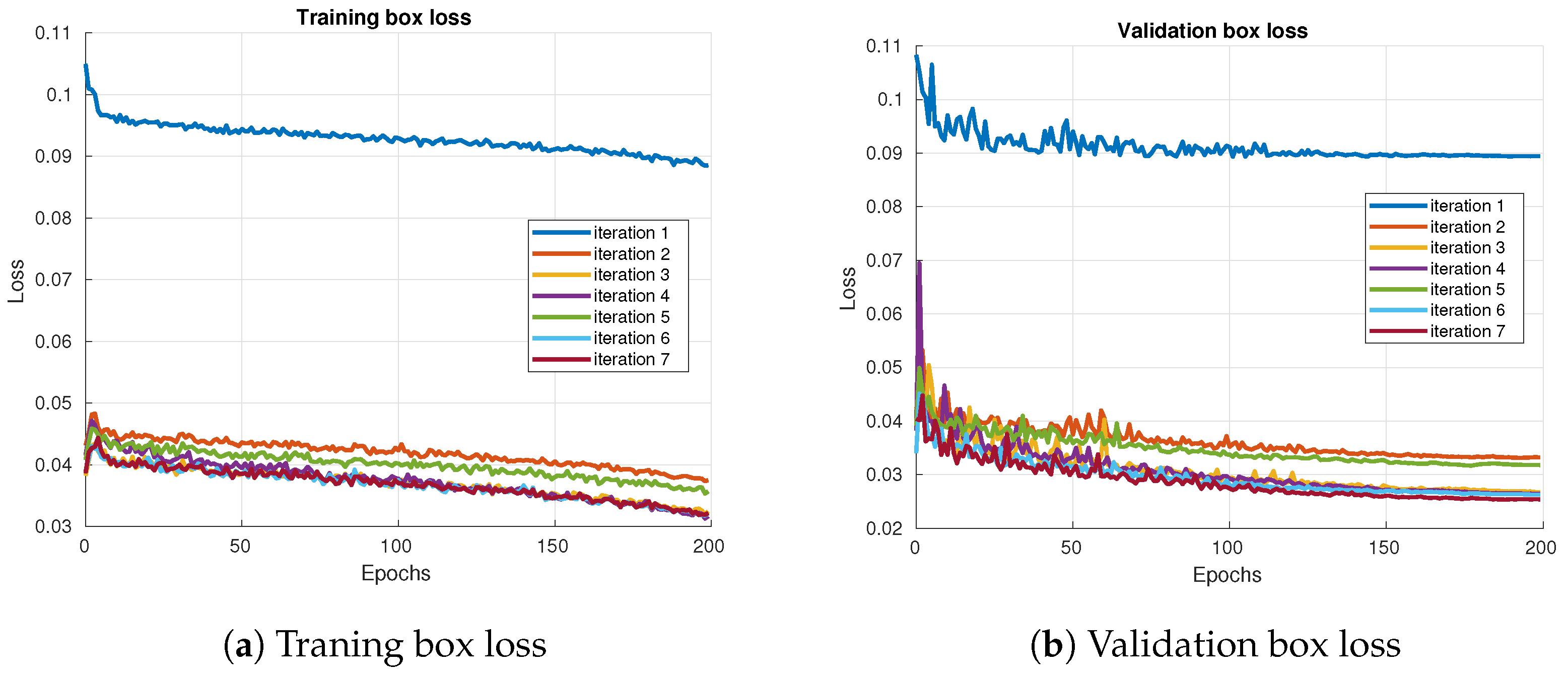
Figure 8a presents the Loss of the Training Box, measuring the accuracy of the bounding boxes in the training dataset, indicating which of the predicted boxes best matches the actual boxes of the object. Figure 8b shows the loss of the validation box, which evaluates the precision of the bounding boxes in the validation dataset. This metric evaluates the precision of the boxes in data not seen during training.

Among all iterations, iteration 1 shows the worst results. From there, an improvement is observed up to iteration 3. However, from iteration 4 to iteration 7, the upgrades are inconsistent; some iterations show improvements, while others exhibit slight deteriorations, though not significantly deviating from previous iterations except for iteration 1. This inconsistency is a result of relabeling, a process that, in some cases, introduces false positives in the validation and training datasets, causing slight variations in the metrics.

Once each iteration’s training was completed under the same conditions and with the same number of epochs, a comparison was made using the test dataset. It is important to note that no training had contact with this set, which was also correctly labeled, allowing for a comparative analysis in each iteration. Metrics such as mAP-50, mAP-50:90, Precision (P), and Recall (R) were calculated. The P metric indicates the model’s predictions, that is, the percentage of correct predictions out of the total predictions made. The R metric indicates the model’s ability to identify all positive instances, i.e., the percentage of actual positive cases detected by the model. The mAP-50 metric considers a detection to be correct if the overlap (IoU) between the prediction and the detection box is at least 0.5. In contrast, the mAP-50:90 metric considers correct detections over a range of overlaps from an IoU of 0.5 to 0.95.

3.2. Recursive Estimation and Metric Modeling

3.2.1. Parameter Definitions in Metric Models

We present the mathematical variables specifically employed in the modeling and analysis of metric behavior throughout the recursive estimation process. These variables are used to characterize the system’s performance across successive iterations.

• i: The iteration index, where $i\in \{1,2,\dots ,7\}$.
• $Y_P$: Fitted model output for the Precision Metric across iterations.
• $Y_R$: Fitted model output for the Recall Metric across iterations.
• $Y_{\mathrm{mAP}\text{-}50}$: Fitted model output for the mAP at an IoU threshold of 0.50.
• $Y_{\mathrm{mAP}\text{-}50:90}$: Fitted model output for the mean Average Precision over IoU thresholds from 0.50 to 0.95.
• $R^2\in [0,1]$: Coefficient of determination indicating the goodness-of-fit of the model to the empirical data. Values closer to 1 indicate a better fit.

These variables are central to understanding the empirical behavior of the labeling correction strategy and the evolution of model performance throughout iterative refinement.

3.2.2. Metric Model Estimation

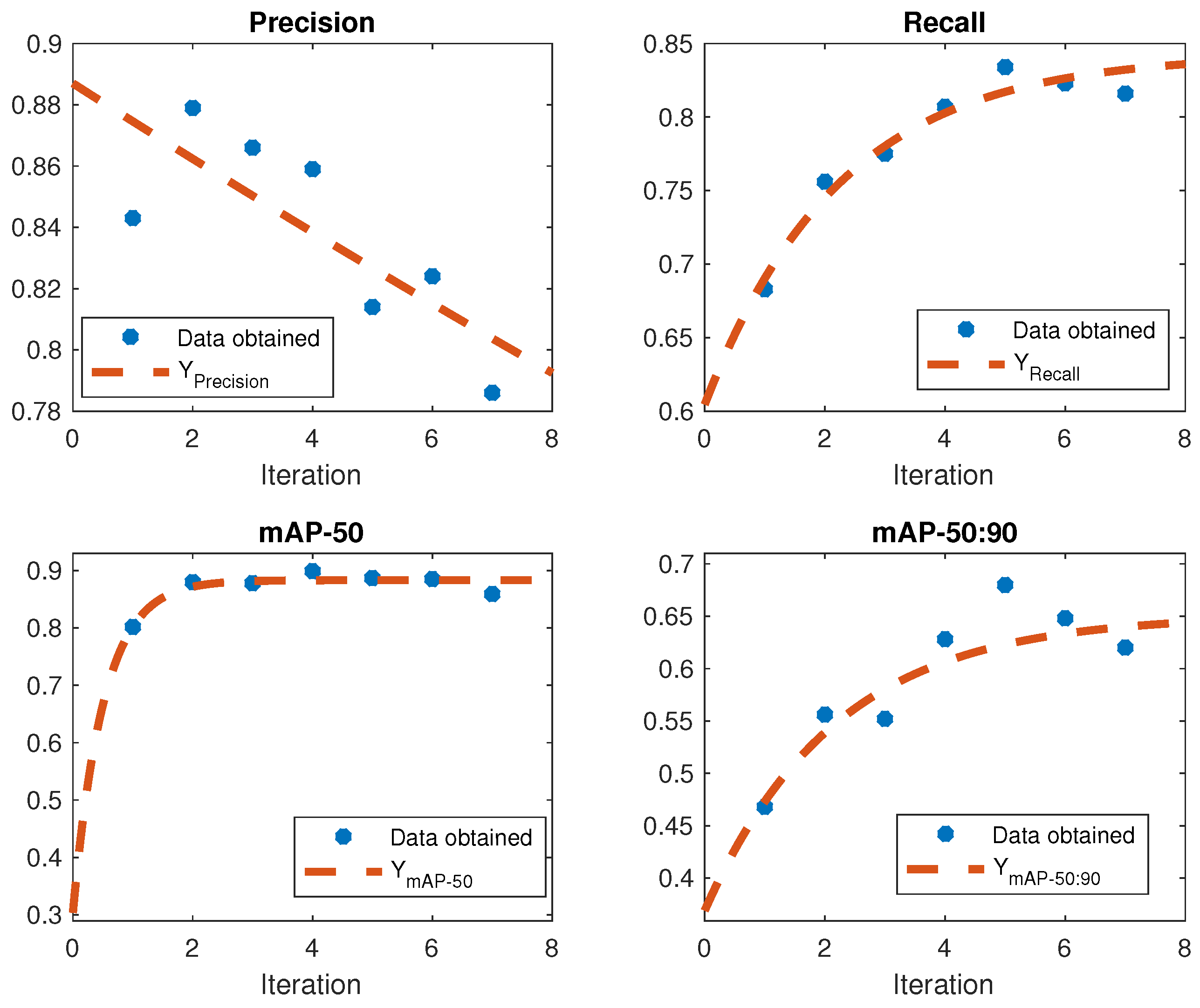
After completing seven iterations, as detailed in Section 3.2.2, the results for the four metrics—Precision, Recall, mAP-50, and mAP-50:90—were obtained. These results, previously mentioned, are shown in Figure 9. It can be seen that all the metrics increased in the first iteration but varied subsequently. The metric shows a downward trend. To confirm this behavior, we developed mathematical models for each metric based on the experimental results, allowing for an analysis of their behavior over time. The mathematical models obtained for each metric are as follows:

$$Y_P=0.0006+0.8864e^{-0.01409i}$$

(18a)

$$Y_R=0.8427-0.2381e^{-0.4463i}$$

(18b)

$$Y_{mAP\text{-}50}=0.8833-0.5798e^{-1.9618i}$$

(18c)

$$Y_{mAP\text{-}50:90}=0.6511-0.2821e^{-0.4608i}$$

(18d)

where i denotes the iteration, $Y_P$ represents the variation in the metric value per epoch of the Precision, $Y_R$ represents the variation in the metric value per epoch of the Recall, $Y_{mAP\text{-}50}$ signifies the variation in the metric value per epoch of the mAP-50 metric, and $Y_{mAP\text{-}50:90}$ denotes the variation in the metric value per epoch of the mAP-50:90 metric. The graphical representations of the mathematical models obtained, along with the corresponding values of these metrics, are depicted in Figure 9. To assess the precision of the models, the determination coefficients $R^2$ indicate the strength of the relationship between our experimental data and the models generated from Equations (18a)–(18d). The accuracy of each fitted model is evaluated using the coefficient of determination $R^2$, which quantifies how well the model predictions approximate the actual metric values across iterations. The values of $R^2$ for each metric model are summarized in

Table 1. Table depicting the calculations of determination coefficients for the model derived from the metrics data.

	${\mathit{Y}}_{\mathit{P}}$	${\mathit{Y}}_{\mathit{R}}$	${\mathit{Y}}_{\mathit{mAP}\text{-}50}$	${\mathit{Y}}_{\mathit{mAP}\text{-}50:90}$
$R^2$	0.6097	0.9534	0.8497	0.8253

, providing a numerical validation of the models’ explanatory capacity.

Table 1 displays determination coefficients with a value of 0.6097 for the mathematical model that predicts the metric variation in each iteration, 0.9534 for the model that predicts the Recall Metric variation of each iteration, 0.8497 for the model that predicts the mAP-50 metric variation, and 0.8253 for the model that predicts the mAP-50:90 metric variation in every iteration. The lowest coefficient, represented by the Precision Metric at 0.6097, signifies that the variability of the dependent variable can be accounted for by the independent variables within the model at 60.97%. The model thus provides a significant explanation for most of the data’s variability. In contrast, the remaining 39.03% variability needs to be accounted for due to the inability to quantify the potential false positives the algorithm may generate in every iteration within both the validation and training datasets. However, the remaining metrics exceed 80%, suggesting a strong fit of the corresponding models. By examining these values along with Equations (18a)–(18d) in the mathematical model, an inference can be drawn stating that increasing the number of iterations in image labeling could result in 60.97% chances that the metric reaches 0.0006, a 95.34% probability of the Recall Metric hitting 0.8427, an 84.97% possibility of the mAP-50 metric reaching 0.8833, and an 82.53% probability of the mAP-50:90 metric obtaining 0.6511. This implies that, with multiple iterations of the Precision Metric (P), the model might yield a small number of incorrect predictions relative to the overall optimistic predictions made. However, it may also lead to an increase in the generation of false positives. Alternatively, the Recall Metric (R) indicates the model’s ability to encompass most positive cases within the dataset. Currently, the mAP-50 metric implies a robust and accurate model, particularly in terms of positive instances. In addition, the mAP-50:90 metric indicates enhanced robustness of the model in terms of object detection across a more comprehensive range of confidence thresholds.

3.3. Generalization and Evaluation Consistency

In this study, we chose to employ the YOLOv5 detector architecture both for the filtering process and for performance evaluation across all iterations. This decision was guided by the need for experimental consistency and the desire to isolate the effects of the label correction methodology. Using a single architecture eliminates confounding factors that might arise from architectural or training differences, thereby allowing a clearer interpretation of the impact of iterative label refinement.

Moreover, the evaluation was conducted on an independently labeled test set, which was excluded from all training and filtering procedures. This served as an unbiased benchmark for assessing the generalization capability of the filtered dataset.

While testing with a different detector architecture (e.g., Faster R-CNN or SSD) could further reinforce the robustness of our approach, we reserve this as future work. Our current strategy allows us to attribute observed performance gains specifically to the proposed filtering mechanism, without interference from differences in model structures or capacities.

Recursive Estimation Analysis

The tomato detection model showed a notable performance boost with the filter’s use. While Precision slightly decreased, the Recall (R), mAP-50, and mAP-50:90 metrics saw significant improvements. See

Table 2. Test performance of the variants of the method for label replacement. The best values are remarked.

Method	Precision	Recall	mAP-50	mAP-50:90
Yolo Original	0.84	0.68	0.8	0.46
Filtered Yolo (Replacement)	0.79	0.82	0.86	0.63

. This indicates that the model can now detect more tomatoes in images, even under challenging conditions.

To further assess the reliability of these improvements, we analyzed the coefficient of determination ($R^2$) for the fitted models describing the evolution of each metric. As detailed in Table 1, the Recall and mAP metrics exhibit high $R^2$ values (above 0.82), confirming that the proposed models capture the underlying performance trends effectively. This provides quantitative support for the improvements observed in the iterative filtering process and aligns with the empirical data shown in Figure 9.

However, the auto-filtering method may introduce false positives. In summary, the filter improves detection, which is crucial for precision agriculture, by accurately identifying crops. It is recommended that the iterations be limited to four to prevent false positives.

To address potential overfitting from recursively regressing the same model, we evaluated all iterations using a fully independent and manually verified test set, as described in Section 2.3. This test set was never exposed during training or label correction and thus served as an external benchmark to assess generalization. Future work will incorporate datasets from different greenhouse environments to further validate robustness.

4. Conclusions

We have proposed an iterative relabeling approach for dataset correction. The goal of this approach is to correct errors in the dataset caused by incorrect annotations. This method relabels the training dataset over several iterations. Significant improvements were observed, particularly between the first and second iterations. However, in subsequent iterations, the improvements stabilized and occasionally decreased due to an increase in false positives, though the performance remained superior to that of the original dataset.

To comprehensively evaluate the effectiveness of the model, we employed various metrics, such as Precision (P), Recall (R), mAP-50, and mAP-50:90. By formulating mathematical models to analyze metric trends, we observed that both mAP-50 and mAP-50:90 improved with each new iteration. However, these improvements were limited, reaching values of 0.8833 for mAP-50 and 0.6511 for mAP-50:90. This indicates enhanced detection of tomatoes but also an increase in false positives as Precision decreased over multiple iterations. Despite this, the labeling of the database improved significantly. The mathematical models derived from the metrics of each iteration provided a detailed and reliable understanding of the performance of the model, allowing us to reach this conclusion.

The results of our research suggest that relabeling enhances detection capabilities and highlights the challenge of false positives. To address this issue, we recommend limiting the iterations to four to avoid an excess of false positives and to develop an efficient model with a well-labeled dataset. This research demonstrates significant performance advances with practical applications, such as precision agriculture, where accurate crop identification is crucial for informed decision making. This underscores the relevance of our work to the field of precision agriculture.

In future research, we will test different ways to merge the corrected labels with the original data. In addition, we will test the approach in contexts different from agriculture.