
Reconstruction, Segmentation and Phenotypic Feature Extraction of Oilseed Rape Point Cloud Combining 3D Gaussian Splatting and CKG-PointNet++


Abstract
1. Introduction
2. Materials and Methods
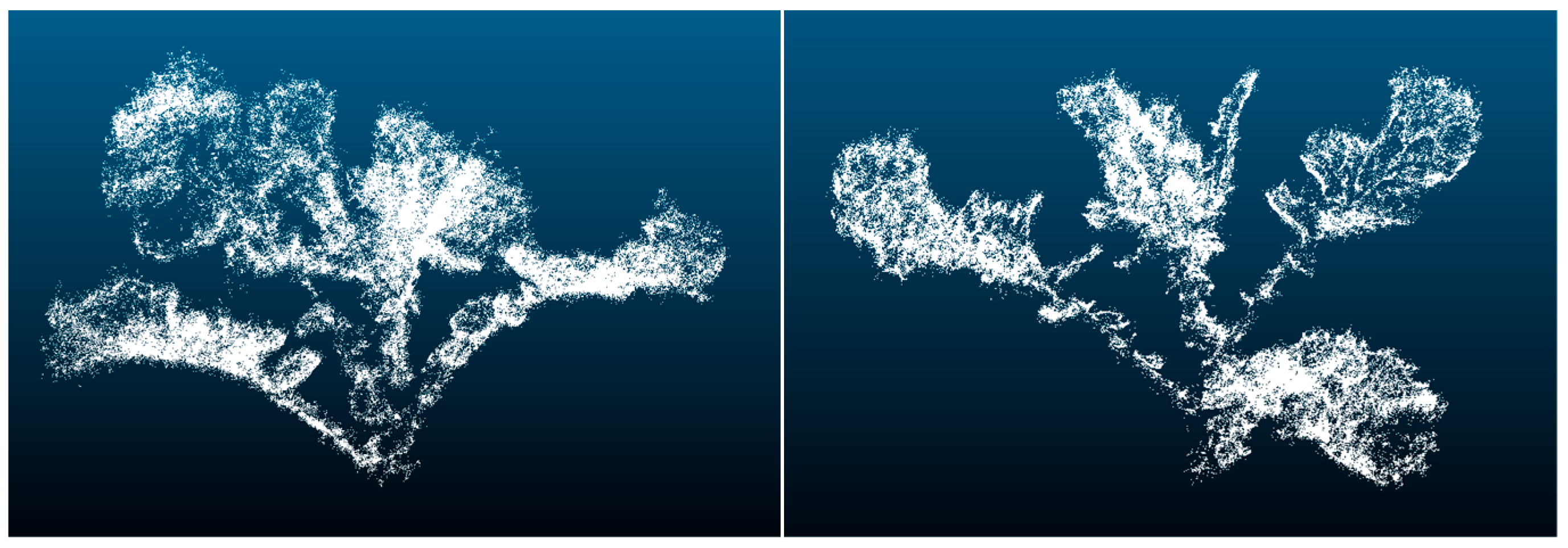
- Collecting multi-view image sets of oilseed rape and inputting them into Gaussian Splatting pipeline for processing, and generating Gaussian point clouds representing the 3D morphology of the plants through dense modeling of the scene and Gaussian voxelization.
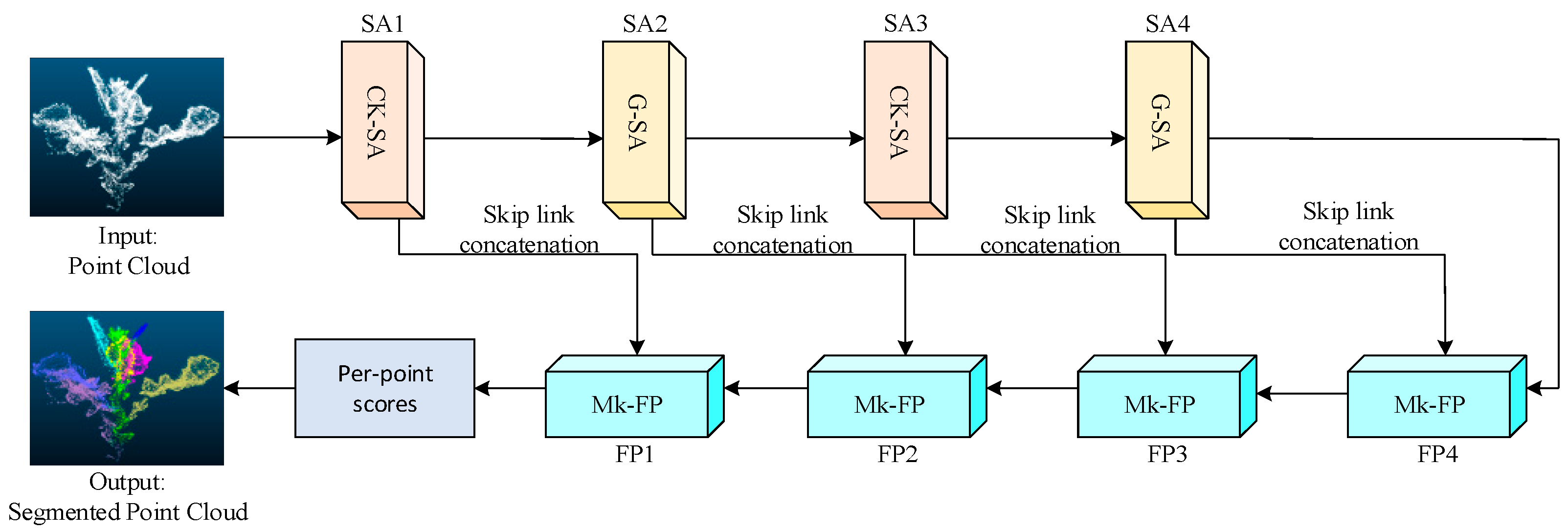
- A preprocessing step is performed on the generated point cloud, combining statistical outlier removal (SOR) [33] and radius outlier filter (ROL) [34] to remove noisy and abnormal point clouds, and then using the RANSAC [35] algorithm to segment the target plant point cloud. Based on the preprocessed point cloud, segmentation is performed using the improved CKG-PointNet++ model. The fine-grained geometric and local semantic information in the point cloud is effectively captured at the feature extraction (SA) layer, and the global information is gradually integrated while maintaining the local details. The local information is effectively integrated with the global context in the feature propagation (FP) layer to improve the overall expression capability and segmentation accuracy.
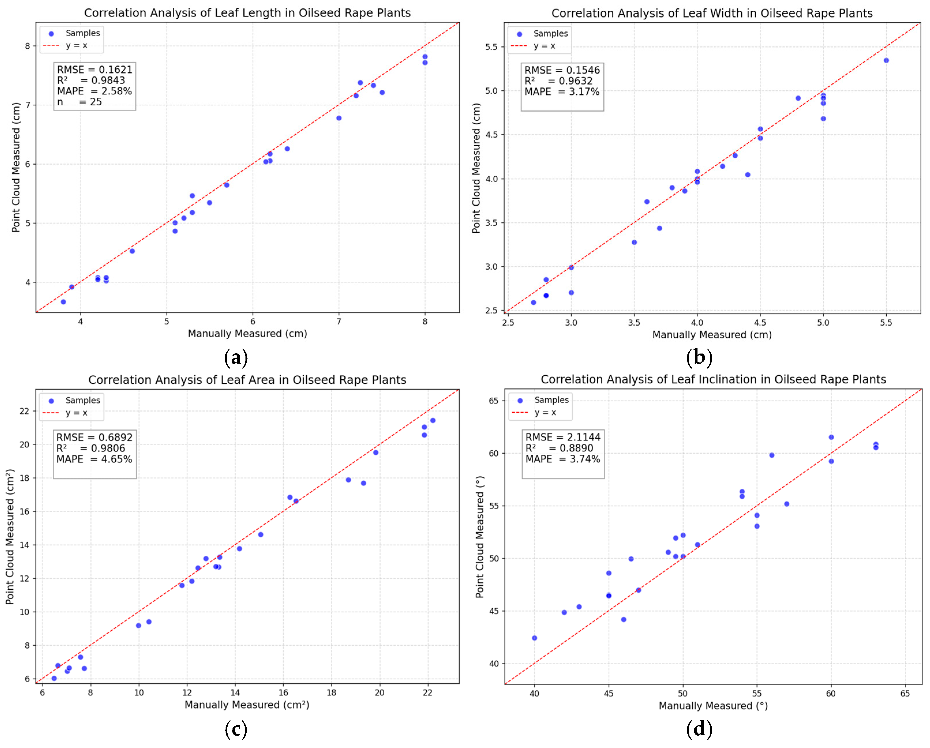
- Key phenotypic features, such as plant height, leaf length, leaf width, leaf area and leaf inclination, were calculated based on the segmented oilseed rape point cloud. The results are compared and analyzed with the real measured phenotypic parameters to assess the measurement accuracy and reliability of the process.
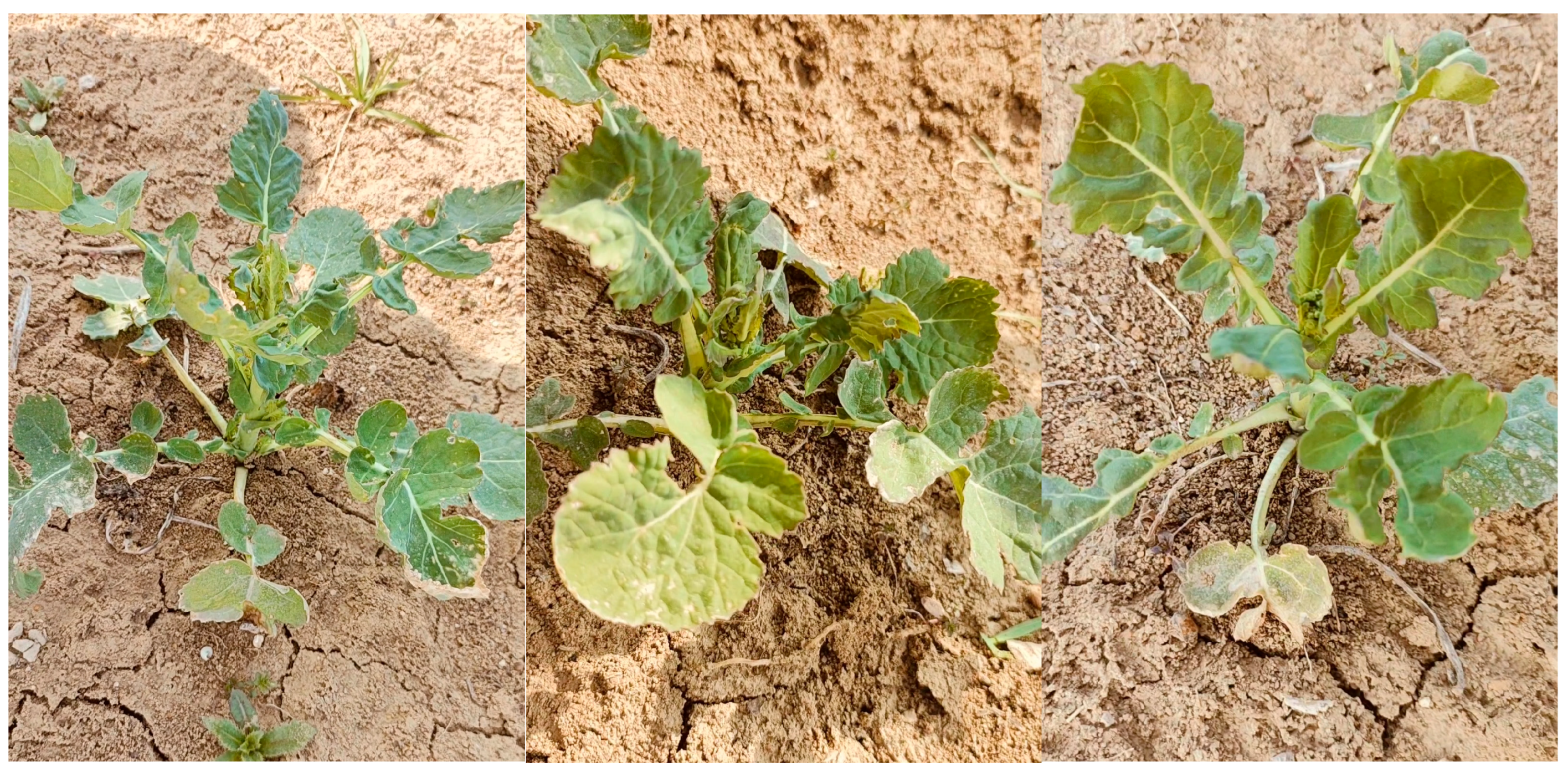
2.1. Oilseed Rape Data Collection
2.2. Oilseed Rape Point Cloud Generation
2.2.1. 3D Reconstruction of Point Clouds
2.2.2. Point Cloud Processing
2.3. Oilseed Rape Point Cloud Segmentation Model
2.3.1. CKG-PointNet++
- Feature Extraction (Set Abstraction, SA) Layer. It uses furthest point sampling (FPS) to select a set of representative sampling points from the original point cloud, and uses ball query to construct local regions from the sampling points and nearby points. Local feature extraction is performed in each local region, a multilayer perceptron is used to transform the features of the local points, and the local feature representations are aggregated through the max pooling operation.
- 2
- Feature Propagation (FP) Layer: The FP layer samples the low-resolution abstract features back to the original point cloud size, and fuses the fine-grained information from the earlier SA layers mainly through interpolation and cross-layer hopping connections to generate the final feature representation for each point. This is finally fed into the multilayer perceptron (MLP) for segmentation prediction.
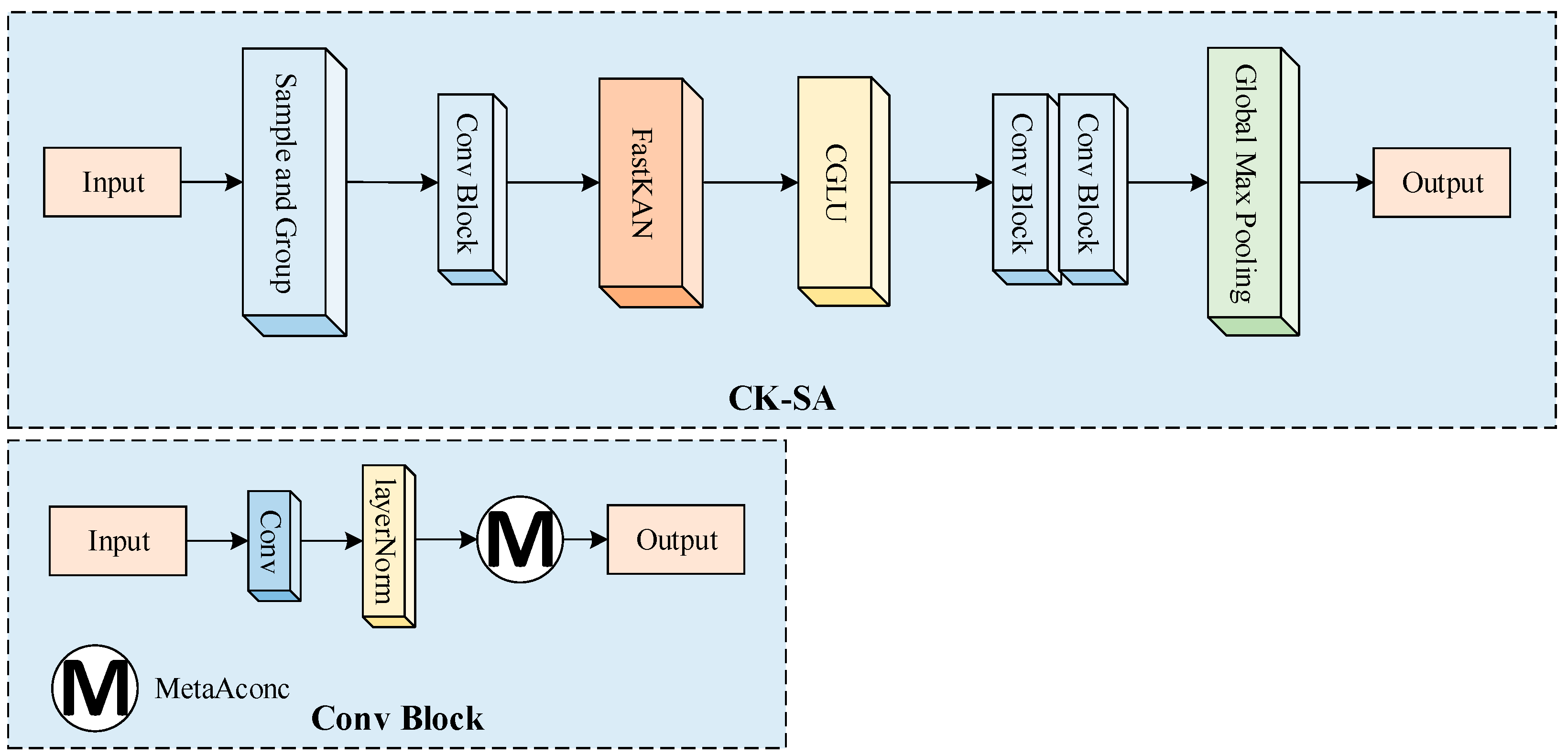
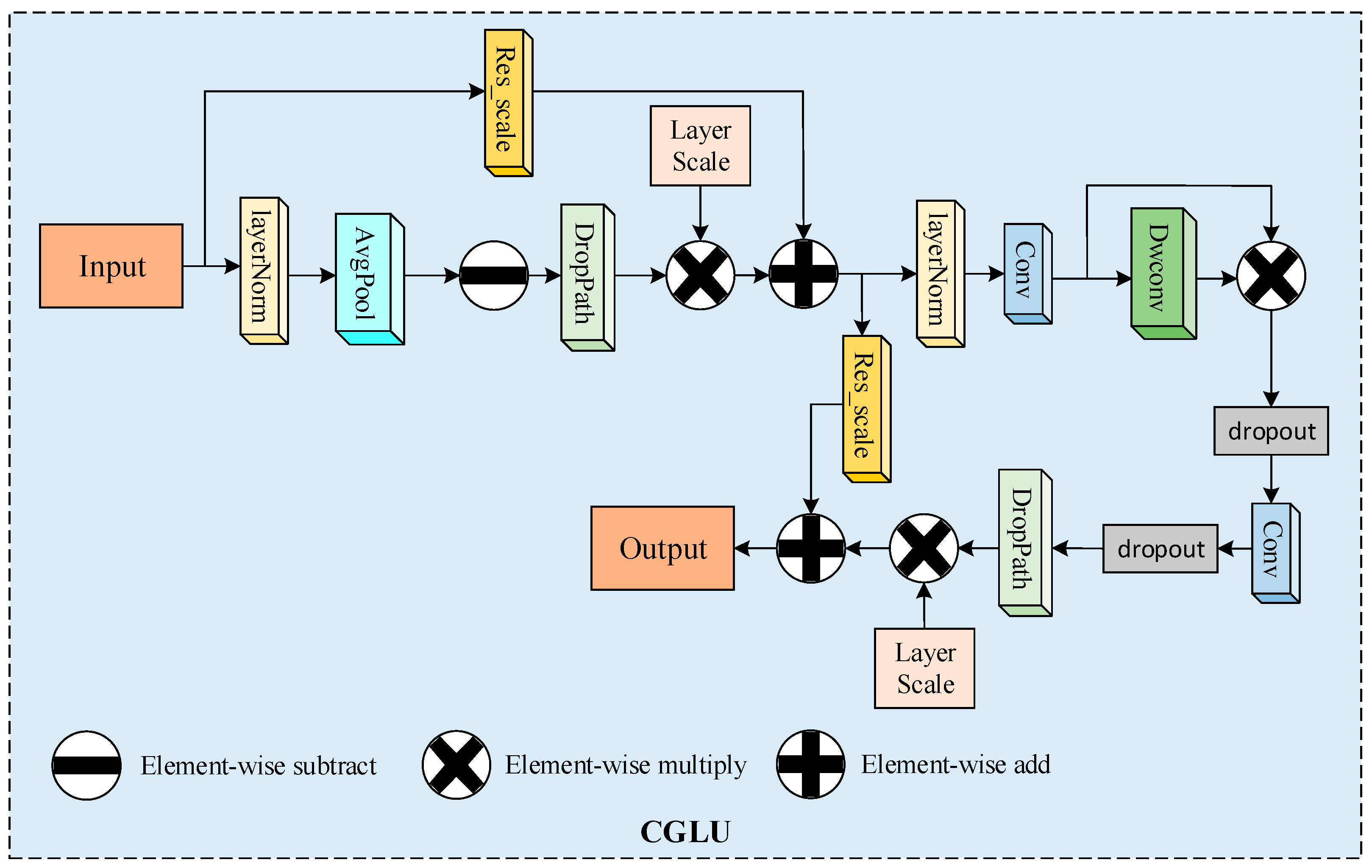
2.3.2. CK-SA
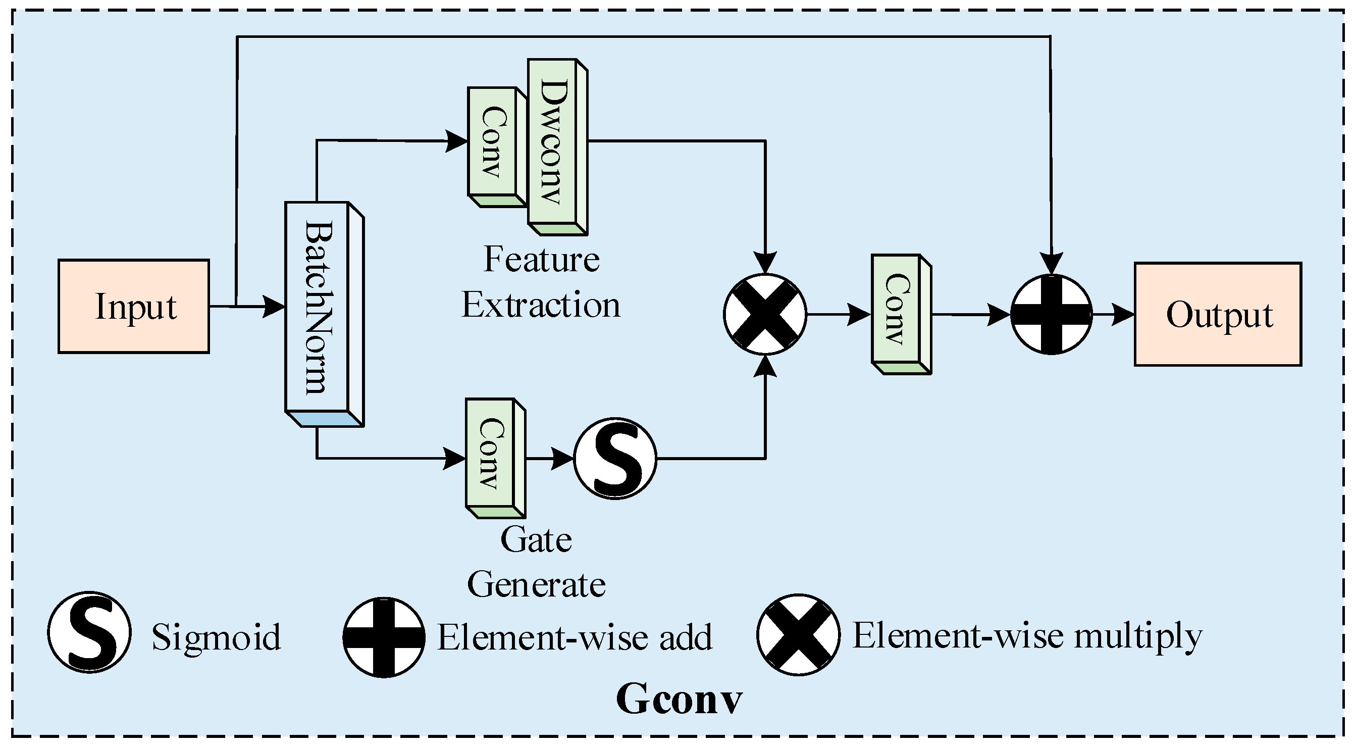
2.3.3. G-SA
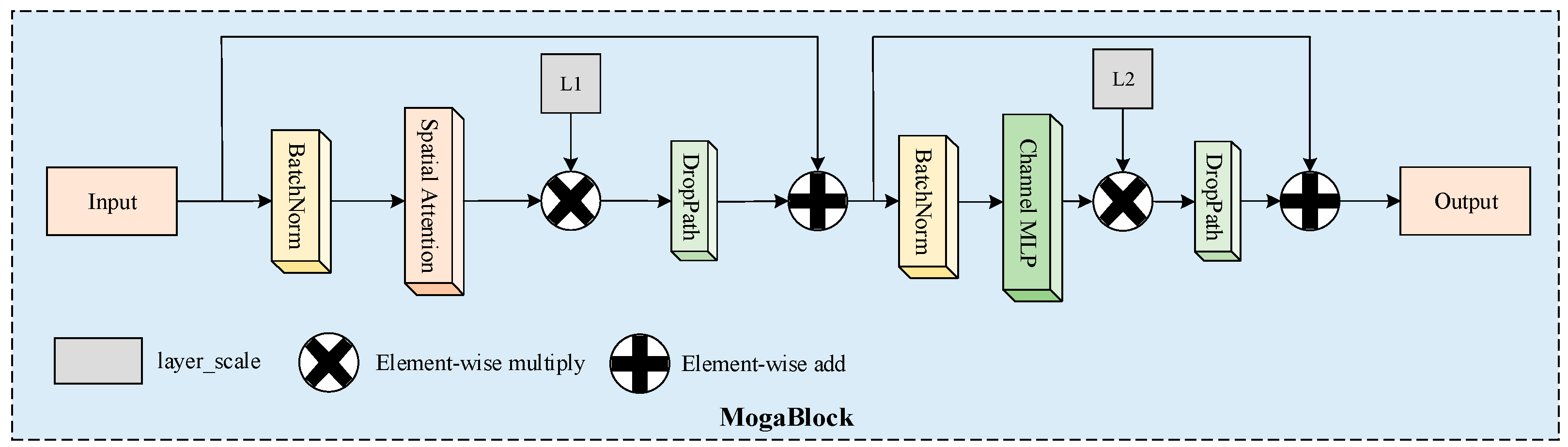
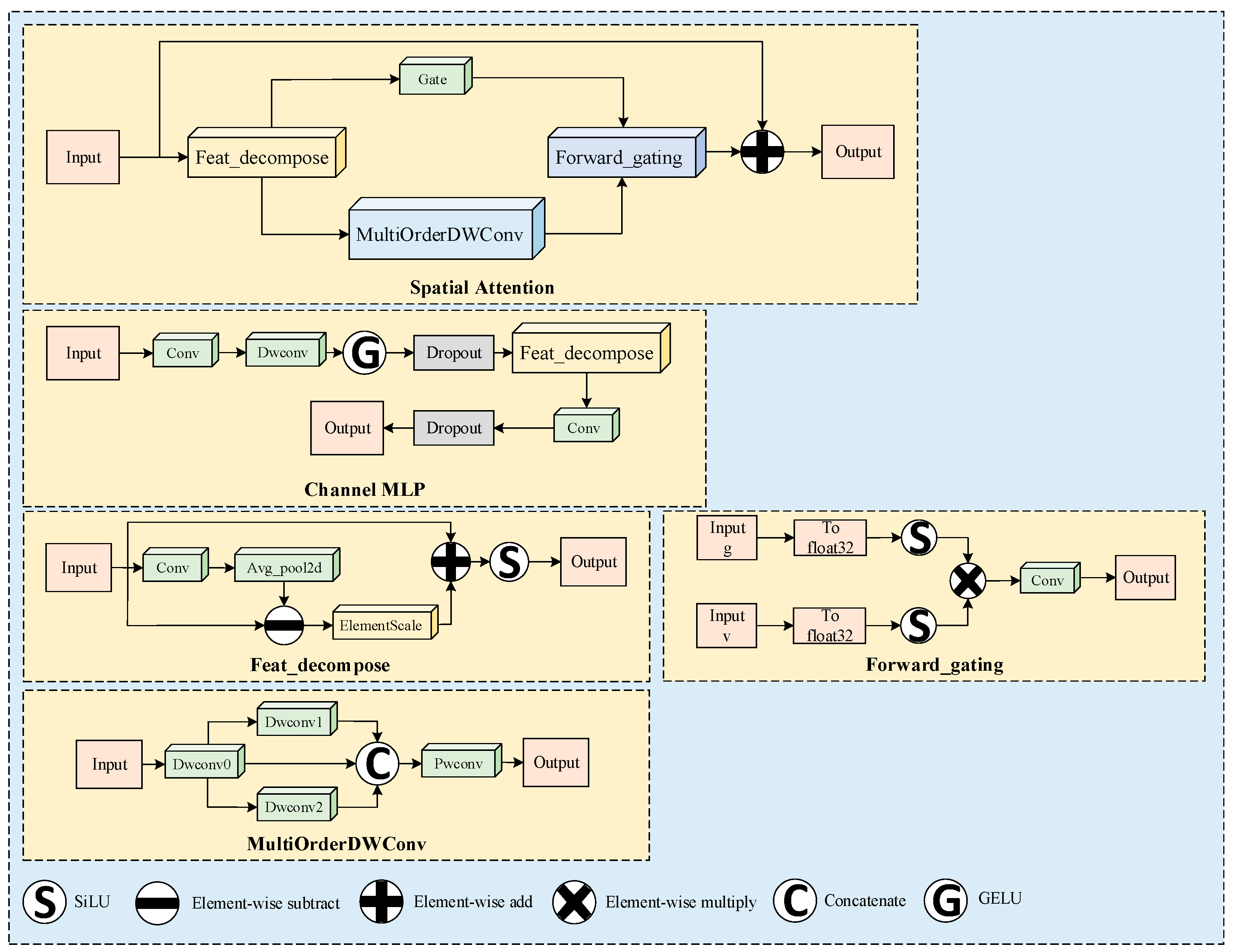
2.3.4. FP-Moga
2.3.5. FP-Self-Attention
2.4. Model Training and Performance Evaluation
- (1)
- Model Training Parameters
- (2)
- Three-dimensional Reconstruction Evaluation
- (3)
- Semantic Segmentation Evaluation
- (4)
- Evaluation of phenotypic parameter measurements
3. Results
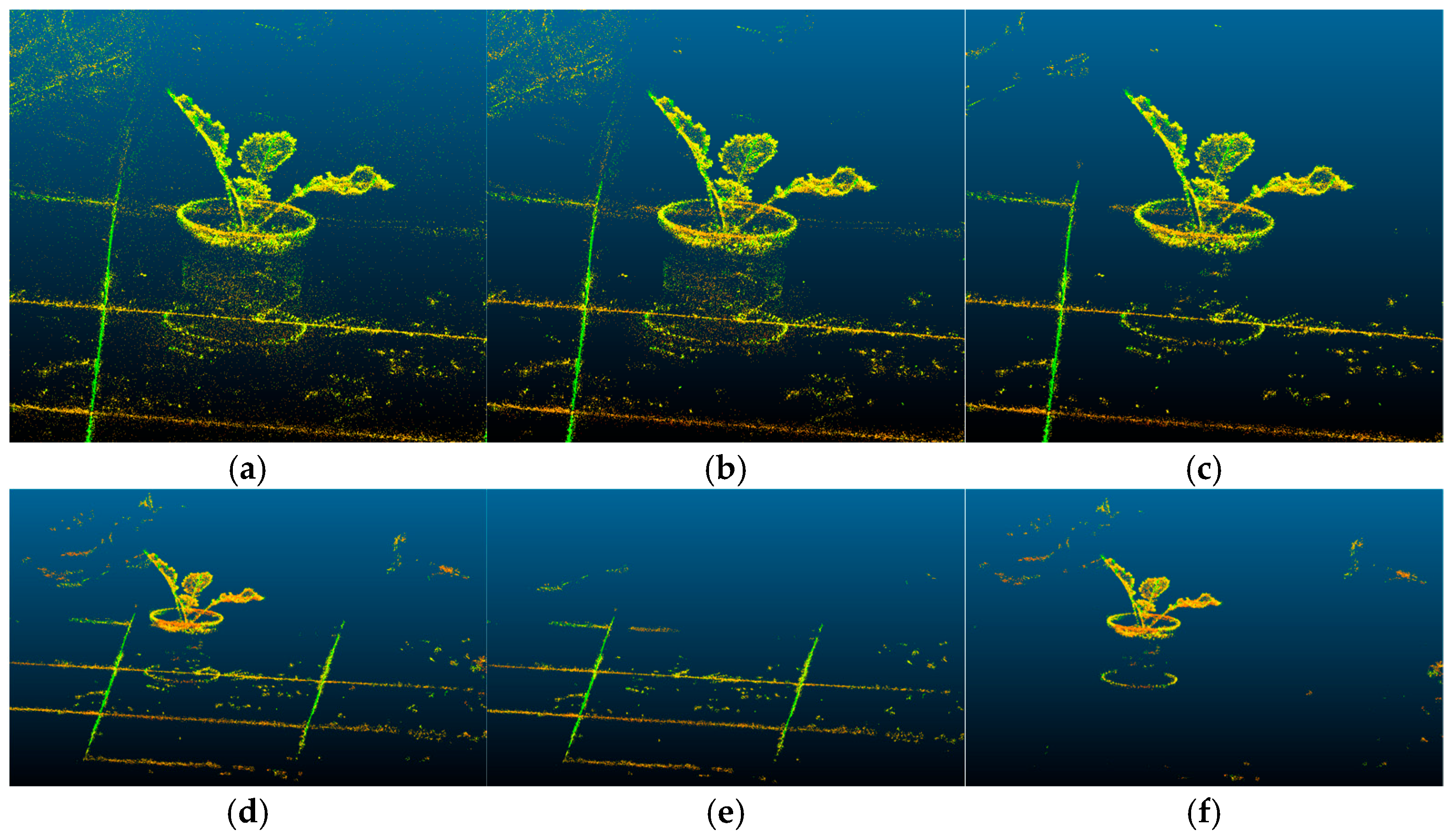
3.1. 3D Gaussian Splatting Reconstruction
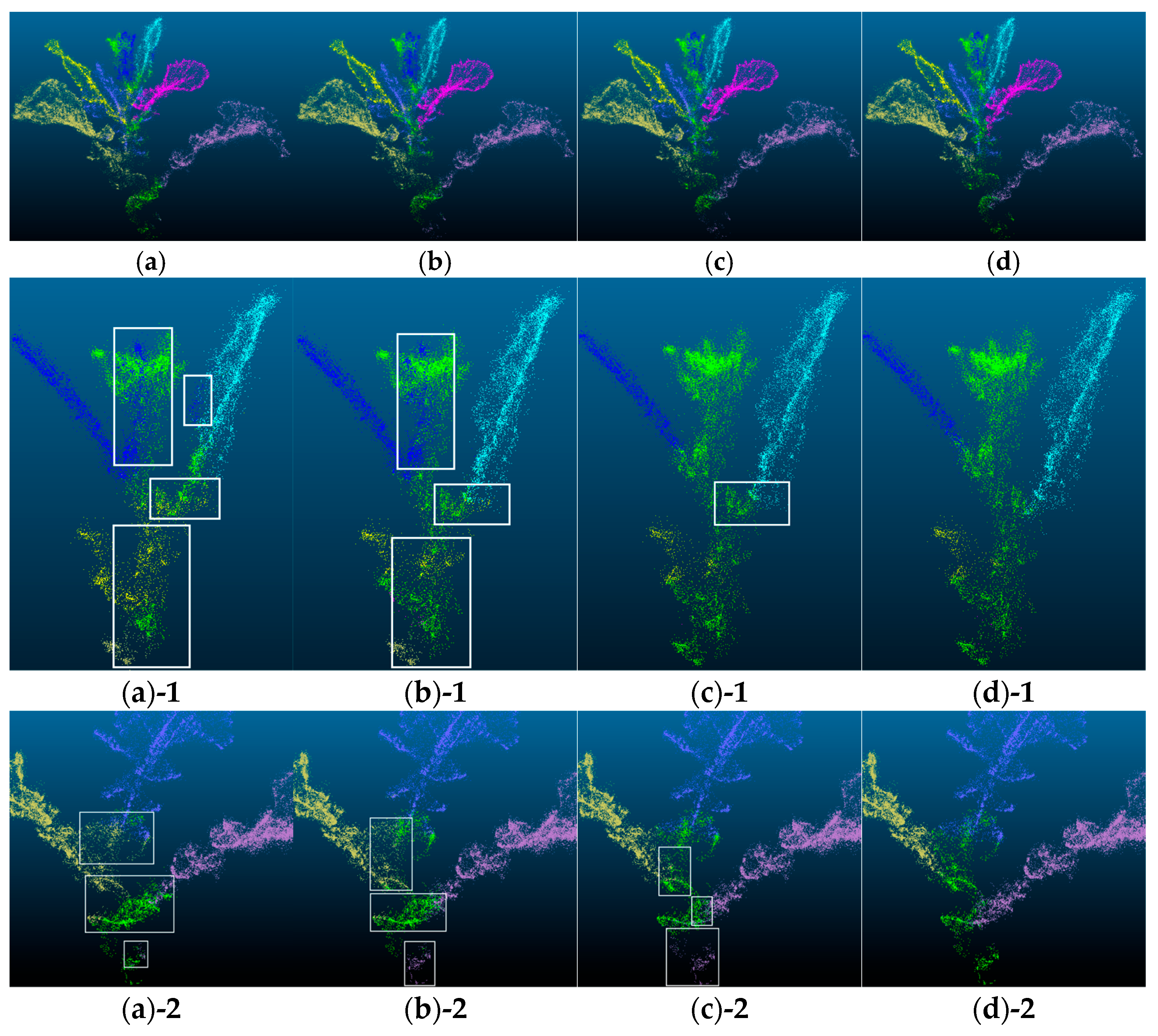
3.2. Point Cloud Segmentation Results
3.3. Calculation of Phenotypic Parameters
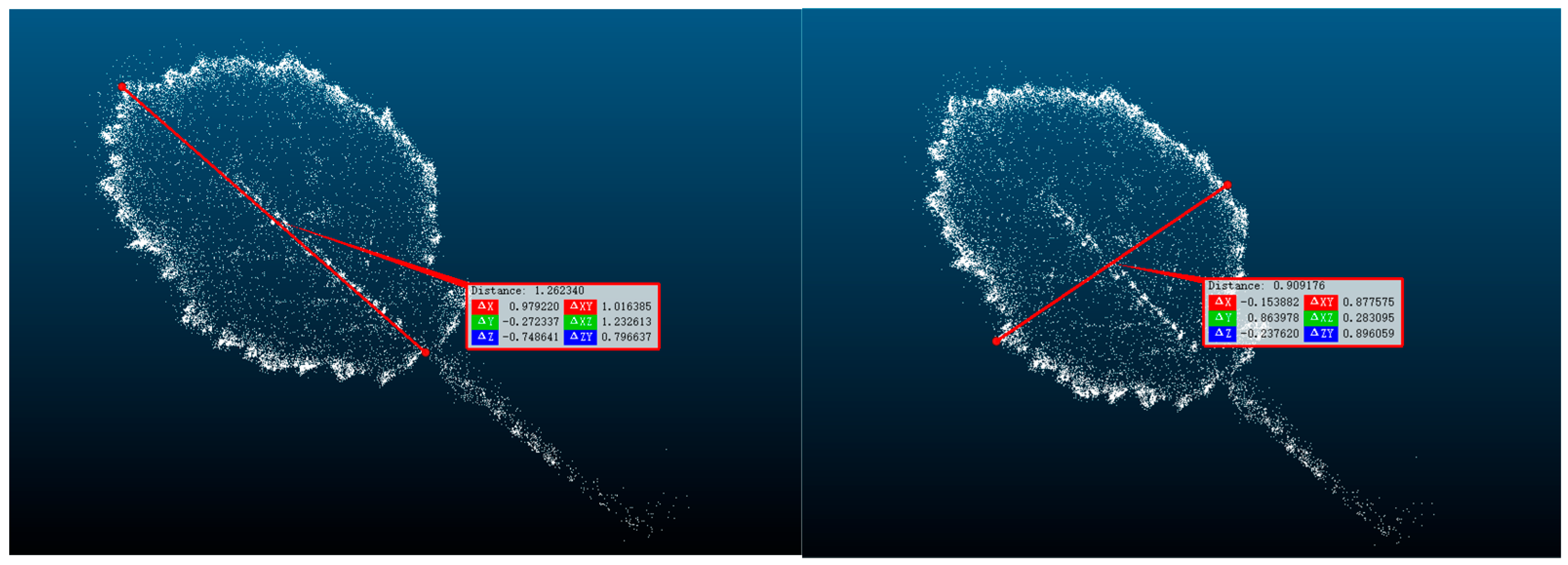
3.3.1. Oilseed Rape Point Cloud Processing
3.3.2. Calculation of Oilseed Rape Phenotypes
4. Discussion
5. Conclusions
Author Contributions
Funding
Institutional Review Board Statement
Data Availability Statement
Conflicts of Interest
References
- Fang, Z.; Liu, P. The source of capacity improvement of China’s three major oilseed crops. Chin. J. Oilseed Crops 2025, 47, 243–259. [Google Scholar]
- Fu, D.-H.; Jiang, L.-Y.; Mason, A.S.; Xiao, M.-L.; Zhu, L.-R.; Li, L.-Z.; Zhou, Q.-H.; Shen, C.-J.; Huang, C.-H. Research progress. J. Integr. Agric. 2016, 15, 1673–1684. [Google Scholar] [CrossRef]
- Wang, H. Development strategy of oilseed rape industry oriented to new demand. Chin. J. Oilseed Crops 2018, 40, 613. [Google Scholar]
- Hu, Q.; Hua, W.; Yin, Y.; Zhang, X.; Liu, L.; Shi, J.; Zhao, Y.; Qin, L.; Chen, C.; Wang, H. Rapeseed research and production in China. Crop J. 2017, 5, 127–135. [Google Scholar] [CrossRef]
- Li, H.; Feng, H.; Guo, C.; Yang, S.; Huang, W.; Xiong, X.; Liu, J.; Chen, G.; Liu, Q.; Xiong, L.; et al. High-throughput phenotyping accelerates the dissection of the dynamic genetic architecture of plant growth and yield improvement in rapeseed. Plant Biotechnol. J. 2020, 18, 2345–2353. [Google Scholar] [CrossRef]
- Zhang, H.; Wang, L.; Jin, X.; Bian, L.; Ge, Y. High-throughput phenotyping of plant leaf morphological, physiological, and biochemical traits on multiple scales using optical sensing. Crop J. 2023, 11, 1303–1318. [Google Scholar] [CrossRef]
- Li, Y.; Wen, W.; Miao, T.; Wu, S.; Yu, Z.; Wang, X.; Guo, X.; Zhao, C. Automatic organ-level point cloud segmentation of maize shoots by integrating high-throughput data acquisition and deep learning. Comput. Electron. Agric. 2022, 193, 106702. [Google Scholar] [CrossRef]
- Guo, W.; Zhou, C.; Han, W. Rapid and non-destructive measurement system of plant leaf area based on Android mobile phone. J. Agric. Mach. 2014, 45, 275–280. [Google Scholar]
- Xiao, Y.; Liu, S.; Hou, C.; Liu, Q.; Li, F.; Zhang, W. Organ Segmentation and Phenotypic Analysis of Soybean Plants Based on Three-dimensional Point Clouds. J. Agric. Sci. Technol. 2023, 25, 115–125. [Google Scholar]
- Yang, X.; Hu, S.; Wang, Y.; Yang, W.; Zhai, R. Cotton Phenotypic Trait Extraction Using Multi-Temporal Laser Point Clouds. Smart Agric. 2021, 3, 51–62. [Google Scholar]
- Liang, X.; Yu, W.; Qin, L.; Wang, J.; Jia, P.; Liu, Q.; Lei, X.; Yang, M. Stem and Leaf Segmentation and Phenotypic Parameter Extraction of Tomato Seedlings Based on 3D Point. Agronomy 2025, 15, 120. [Google Scholar] [CrossRef]
- Yang, Z. Research and Implementation of a Phenotypic Measurement System for Wolfberry Plants Based on Three-Dimensional Reconstruction. Master’s Thesis, Ningxia University, Ningxia, China, 2022. [Google Scholar]
- Xu, Q.; Cao, L.; Xue, L.; Chen, B.; An, F.; Yun, T. Extraction of Leaf Biophysical Attributes Based on a Computer Graphic-based Algorithm Using Terrestrial Laser Scanning Data. Remote Sens. 2019, 11, 15. [Google Scholar] [CrossRef]
- Thapa, S.; Zhu, F.; Walia, H.; Yu, H.; Ge, Y. A Novel LiDAR-Based Instrument for High-Throughput, 3D Measurement of Morphological Traits in Maize and Sorghum. Sensors 2018, 18, 1187. [Google Scholar] [CrossRef] [PubMed]
- Yau, W.K.; Ng, O.-E.; Lee, S.W. Portable device for contactless, non-destructive and in situ outdoor individual leaf area measurement. Comput. Electron. Agric. 2021, 187, 106278. [Google Scholar] [CrossRef]
- Li, Y.; Wen, W.; Fan, J.; Gou, W.; Gu, S.; Lu, X.; Yu, Z.; Wang, X.; Guo, X. Multi-source data fusion improves time-series phenotype accuracy in maize under a field high-throughput phenotyping platform. Plant Phenomics 2023, 5, 0043. [Google Scholar] [CrossRef]
- Xu, X.; Li, J.; Zhou, J.; Feng, P.; Yu, H.; Ma, Y. Three-Dimensional Reconstruction, Phenotypic Traits Extraction, and Yield Estimation of Shiitake Mushrooms Based on Structure from Motion and Multi-View Stereo. Agriculture 2025, 15, 298. [Google Scholar] [CrossRef]
- Kerbl, B.; Kopanas, G.; Leimkühler, T.; Drettakis, G. 3D Gaussian Splatting for Real-Time Radiance Field Rendering. ACM Trans. Graph. 2023, 42, 1–14. [Google Scholar] [CrossRef]
- Chen, Y.; Xiong, Y.; Zhang, B.; Zhou, J.; Zhang, Q. 3D point cloud semantic segmentation toward large-scale unstructured agricultural scene classification. Comput. Electron. Agric. 2021, 190, 106445. [Google Scholar] [CrossRef]
- Cui, D.; Liu, P.; Liu, Y.; Zhao, Z.; Feng, J. Automated Phenotypic Analysis of Mature Soybean Using Multi-View Stereo 3D Reconstruction and Point Cloud Segmentation. Agriculture 2025, 15, 175. [Google Scholar] [CrossRef]
- Guo, R.; Xie, J.; Zhu, J.; Cheng, R.; Zhang, Y.; Zhang, X.; Gong, X.; Zhang, R.; Wang, H.; Meng, F. Improved 3D point cloud segmentation for accurate phenotypic analysis of cabbage plants using deep learning and clustering algorithms. Comput. Electron. Agric. 2023, 211, 108014. [Google Scholar] [CrossRef]
- Wang, P.S.; Liu, Y.; Guo, Y.X.; Sun, C.Y.; Tong, X. O-cnn: Octree-based convolutional neural networks for 3d shape analysis. ACM Trans. Graph. TOG 2017, 36, 72. [Google Scholar] [CrossRef]
- Graham, B.; Engelcke, M.; Van Der Maaten, L. 3d semantic segmentation with submanifold sparse convolutional networks. In Proceedings of the IEEE Conference on Computer Vision and Pattern Recognition, Salt Lake City, UT, USA, 18–23 June 2018; pp. 9224–9232. [Google Scholar]
- Meng, H.Y.; Gao, L.; Lai, Y.K.; Manocha, D. Vv-net: Voxel vae net with group convolutions for point cloud segmentation. In Proceedings of the IEEE/CVF International Conference on Computer Vision, Seoul, Republic of Korea, 27 October–2 November 2019; pp. 8500–8508. [Google Scholar]
- Wang, Z.Y.; Sun, H.Y.; Sun, X.P. Survey on Large Scale 3D Point Cloud Processing Using Deep Learning. Comput. Syst. Appl. 2023, 32, 1–12. [Google Scholar] [CrossRef]
- Zhai, Y. Research on 3D Point Cloud Stitching Method Based on Multi-View Camera. Master’s Thesis, Tianjin University of Technology, Tianjin, China, 2022. [Google Scholar]
- Qi, C.R.; Su, H.; Mo, K.; Guibas, L.J. PointNet: Deep learning on point sets for 3d classification and segmentation. In Proceedings of the IEEE Conference on Computer Vision and Pattern Recognition, Honolulu, HI, USA, 21–26 July 2017; pp. 652–660. [Google Scholar]
- Qi, C.R.; Yi, L.; Su, H.; Guibas, L.J. PointNet++: Deep hierarchical feature learning on point sets in a metric space. arXiv 2017, arXiv:1706.02413. [Google Scholar]
- Zhang, C.; Wang, Z.; Wu, H.; Chen, D. Lidar Point Cloud Segmentation Model Based on Improved PointNet++. Laser Optoelectron. Prog. 2024, 61, 0411001. [Google Scholar]
- Guo, M.H.; Cai, J.X.; Liu, Z.N.; Mu, T.J.; Martin, R.R.; Hu, S.M. Pct: Point cloud transformer. Comput. Vis. Media 2021, 7, 187–199. [Google Scholar] [CrossRef]
- Xu, S.; Lu, K.; Pan, L.; Liu, T.; Zhou, Y.; Wang, B. 3D Reconstruction of Rape Branch and Pod Recognition Based on RGB-D Camera. Trans. Chin. Soc. Agric. Mach. 2019, 50, 21–27. [Google Scholar]
- Zhang, L.; Shi, S.; Zain, M.; Sun, B.; Han, D.; Sun, C. Evaluation of Rapeseed Leave Segmentation Accuracy Using Binocular Stereo Vision 3D Point Clouds. Agronomy 2025, 15, 245. [Google Scholar] [CrossRef]
- Rusu, R.B. Semantic 3D object maps for everyday manipulation in human living environments. KI-Künstliche Intell. 2010, 24, 345–348. [Google Scholar] [CrossRef]
- Narváez, E.A.L.; Narváez, N.E.L. Point cloud denoising using robust principal component analysis. In Proceedings of the International Conference on Computer Graphics Theory and Applications, Setúbal, Portugal, 25–28 February 2006; SCITEPRESS: Setúbal, Portugal, 2006; Volume 2, pp. 51–58. [Google Scholar]
- Derpanis, K.G. Overview of the RANSAC Algorithm. Image 2010, 4, 2–3. [Google Scholar]
- Schönberger, J.L.; Frahm, J.-M. Structure-from-Motion Revisited. In Proceedings of the 2016 IEEE Conference on Computer Vision and Pattern Recognition (CVPR), Las Vegas, NV, USA, 27–30 June 2016; pp. 4104–4113. [Google Scholar]
- Shi, D. Transnext: Robust foveal visual perception for vision transformers. In Proceedings of the IEEE/CVF Conference on Computer Vision and Pattern Recognition, Seattle, WA, USA, 16–22 June 2024; pp. 17773–17783. [Google Scholar]
- Li, Z. Kolmogorov-arnold networks are radial basis function networks. arXiv 2024, arXiv:2405.06721. [Google Scholar]
- Song, Y.; Zhou, Y.; Qian, H.; Du, X. Rethinking performance gains in image dehazing networks. arXiv 2022, arXiv:2209.11448. [Google Scholar]
- Li, S.; Wang, Z.; Liu, Z.; Tan, C.; Lin, H.; Wu, D.; Chen, Z.; Zheng, J.; Li, S.Z. Moganet: Multi-order gated aggregation network. arXiv 2022, arXiv:2211.03295. [Google Scholar]
- Wang, P.; Wang, X.; Wang, F.; Lin, M.; Chang, S.; Li, H.; Jin, R. Kvt: K-nn attention for boosting vision transformers. In European Conference on Computer Vision; Springer Nature: Cham, Switzerland, 2022; pp. 285–302. [Google Scholar]
- Wang, Z.; Bovik, A.C.; Sheikh, H.R.; Simoncelli, E.P. Image quality assessment: From error visibility to structural similarity. IEEE Trans. Image Process. 2004, 13, 600–612. [Google Scholar] [CrossRef] [PubMed]
- Dalmago, G.A.; Bianchi, C.A.M.; Kovaleski, S.; Fochesatto, E. Evaluation of mathematical equations for estimating leaf area in rapeseed. Rev. Cienc. Agron. 2019, 50, 420–430. [Google Scholar] [CrossRef]
- Cargnelutti Filho, A.; Toebe, M.; Alves, B.M.; Burin, C.; Kleinpaul, J.A. Estimação da área foliar de canola por dimensões foliares. Bragantia 2015, 74, 139–148. [Google Scholar] [CrossRef]


| Methods | Advantages | Disadvantages | Applicability in Agriculture |
|---|---|---|---|
| Voxel-based methods | Well-structured data and more efficient processing | Presence of voxel quantization errors and loss of detail due to resolution limitations | For modeling the overall morphology of large, structured crops, such as fruit trees |
| 2D projection-based methods | Can use 2D convolutional networks with low computational cost | Significant loss of information in 3D space makes it difficult to capture complex crop structures | Suitable for crop identification in relatively flat areas, such as fields |
| Point-based learning methods | Directly process raw point clouds, preserve geometric structure and have a high accuracy | Sensitive to point count and high computational cost | Suitable for fine-grained segmentation of irregular crops or weeds |
| Model | ITER | Point Number | Loss | L1 | PSNR |
|---|---|---|---|---|---|
| Gaussian Splatting | 7000 | 2,638,272 | 0.134 | 0.0685 | 20.35 |
| Gaussian Splatting | 30,000 | 3,012,945 | 0.082 | 0.0543 | 22.06 |
| Model | AR (%) | Eval Loss | F1 Score | OA (%) | mIoU (%) |
|---|---|---|---|---|---|
| PointNet | 90.95 | 0.235 | 0.911 | 90.73 | 83.60 |
| PointNet++ | 92.99 | 0.191 | 0.931 | 92.80 | 87.15 |
| PointNet_msg | 95.64 | 0.093 | 0.957 | 95.54 | 91.70 |
| CKG-PointNet++ | 98.19 | 0.051 | 0.971 | 97.70 | 96.01 |
| Model | OA (%) | mIoU (%) | Epoch Training Time | Inference Memory (GB) | Peak Training Memory (GB) | Convergence Epochs |
|---|---|---|---|---|---|---|
| PointNet++ | 92.80 | 87.15 | ~4 min | 0.82 GB | 1.46 GB | >20 epochs |
| CKG-PointNet++ | 97.70 | 96.01 | 28 ~ 30 min | 1.66 GB | 5.43 GB | >5 epochs |
| Module | Params (M) | Inference Time (Ms/Sample) | Peak CUDA Memory (MB) |
|---|---|---|---|
| SA (Original) | 0.0038 | 320.66 | 28.36 |
| SA (Improved) | 0.0482 | 333.35 | 54.52 |
| FP (Original) | 0.2637 | 0.84 | 27.06 |
| FP (Improved) | 1.1470 | 2.26 | 40.00 |
| Model | AR (%) | Eval Loss | F1 Score | OA (%) | mIoU (%) |
|---|---|---|---|---|---|
| Base | 92.99 | 0.191 | 0.900 | 92.80 | 87.15 |
| Base+GLUKAN | 97.55 | 0.064 | 0.973 | 97.10 | 94.79 |
| Base+GLUKAN+Moga | 97.77 | 0.062 | 0.975 | 97.26 | 95.13 |
| Base+GLUKAN+Moga+Gconv | 97.74 | 0.057 | 0.976 | 97.35 | 95.26 |
| Base+GLUKAN+Moga+Gconv+Self Attention | 98.19 | 0.051 | 0.971 | 97.70 | 96.01 |
Disclaimer/Publisher’s Note: The statements, opinions and data contained in all publications are solely those of the individual author(s) and contributor(s) and not of MDPI and/or the editor(s). MDPI and/or the editor(s) disclaim responsibility for any injury to people or property resulting from any ideas, methods, instructions or products referred to in the content. |
© 2025 by the authors. Licensee MDPI, Basel, Switzerland. This article is an open access article distributed under the terms and conditions of the Creative Commons Attribution (CC BY) license (https://creativecommons.org/licenses/by/4.0/).
Share and Cite
Huang, Y.; Pang, J.; Yu, S.; Su, J.; Hou, S.; Han, T. Reconstruction, Segmentation and Phenotypic Feature Extraction of Oilseed Rape Point Cloud Combining 3D Gaussian Splatting and CKG-PointNet++. Agriculture 2025, 15, 1289. https://doi.org/10.3390/agriculture15121289
Huang Y, Pang J, Yu S, Su J, Hou S, Han T. Reconstruction, Segmentation and Phenotypic Feature Extraction of Oilseed Rape Point Cloud Combining 3D Gaussian Splatting and CKG-PointNet++. Agriculture. 2025; 15(12):1289. https://doi.org/10.3390/agriculture15121289
Chicago/Turabian StyleHuang, Yourui, Jiale Pang, Shuaishuai Yu, Jing Su, Shuainan Hou, and Tao Han. 2025. "Reconstruction, Segmentation and Phenotypic Feature Extraction of Oilseed Rape Point Cloud Combining 3D Gaussian Splatting and CKG-PointNet++" Agriculture 15, no. 12: 1289. https://doi.org/10.3390/agriculture15121289
APA StyleHuang, Y., Pang, J., Yu, S., Su, J., Hou, S., & Han, T. (2025). Reconstruction, Segmentation and Phenotypic Feature Extraction of Oilseed Rape Point Cloud Combining 3D Gaussian Splatting and CKG-PointNet++. Agriculture, 15(12), 1289. https://doi.org/10.3390/agriculture15121289