Analysis of Carbon Sequestration Capacity and Economic Losses Under Multiple Scenarios in Major Grain-Producing Regions of China: A Case Study of the Urban Agglomeration the Huaihe River Basin

Abstract

The Huaihe River Basin stands as a vital grain-producing base in China. Predicting the dynamic evolution of its carbon storage (CS) is of great theoretical value and practical significance for maintaining regional ecological security, guaranteeing food production capacity, and coping with climate change. This study established a multi-dimensional analysis framework of “scenario simulation–reservoir assessment–value quantification”. Using a sample of 195 cities, the PLUS-InVEST-GIS method was combined to explore the overall CS, spatial differentiation, and value changes in future scenarios. The results indicate that the following: (1) From 2000 to 2020, CS kept on declining, with cultivated land and forest land being the dominant carbon pools, accounting for over 86% of the total CS. (2) From a “city–grid–raster” perspective, the spatial pattern of high-value hot spots of CS remained stable, and the overall pattern remained unchanged under multi-scenario simulation, yet the overall carbon sink center of gravity shifted to the southwest. (3) The top five driving factors are elevation, slope, NDVI, GDP per capita, and population density, accounting for 77.2% of the total driving force. (4) The carbon sequestration capacity at the county scale continued to weaken, and the overall capacity presented the following order: 2035 Farmland protection scenario (FPS) > 2035 Natural development scenario (NDS) > 2035 Urban development scenario (UDS). The resulting carbon economic losses were USD 2.28 × 10⁸, 4.57 × 10⁸, and 6.90 × 10⁸, respectively. The research results will provide scientific land use decision-making support for the realization of the “double-carbon” goals in the Huaihe River grain-producing area.

1. Introduction

Global climate change has emerged as a critical challenge confronting governments worldwide, garnering significant attention due to its profound practical implications [1]. Ecosystems possess remarkable carbon sequestration capacity (CSC) and serve as the planet’s primary carbon sink, playing a pivotal role in mitigating climate anomalies [2,3]. Terrestrial ecosystems are not only an important part of the global ecosystem but also an important carbon reservoir of the Earth’s surface system and participate in the global carbon cycle [4,5]. Terrestrial ecosystems mainly absorb carbon from the air through photosynthesis and sequester it in vegetation and soil, alleviating the greenhouse effect and maintaining ecosystem stability [6]. Land cover is an important factor affecting the CS of terrestrial ecosystems. By analyzing the evolution of land use, we can obtain the temporal and spatial distribution characteristics of CS. This discovery holds substantial importance for alleviating global climate change [1].

In recent years, numerous scholars have carried out extensive research on CS estimation in various regions. The primary methods involve the sample-site measurement method [7,8], model simulation [9,10,11], and biomass inventory [12,13] for CS assessment. However, sample measurements and biomass inventories are limited to small-scale assessments [14,15]. This method is time-consuming and labor-intensive and requires a lot of field investigation work. Additionally, it cannot reveal changes in the spatial and temporal characteristics of CS throughout the entire region. Therefore, many scholars adopt model simulation methods for CS assessment, such as the CASA model [16,17], Biome-BGC model [18,19,20], and InVEST model [14,15,21]. Among these, the InVEST model features a built-in carbon value estimation module and has gained widespread application due to its advantages, such as low data requirements and spatial visualization capabilities. For multi-scenario simulation (MSS) research on land, the main models are the CLUE-S model [22,23], CA model [24,25], PLUS model [26,27,28], etc. Among them, the PLUS model has the advantages of high visualization and accurate MSS. In the study of driving factors, scholars often use regression analysis [29], principal component analysis [30], an Optimal Geodetector (OPGD), and Multi-scale Geographically Weighted Regression (MGWR) to conduct research. Among them, OPGD [31,32,33] immune collinearity can detect interactions between factors. MGWR [34] is more effective in measuring the spatial heterogeneity of factors. This study therefore integrates the PLUS-InVEST coupled model for MSS-based CS quantification and net value change analysis, complemented by OPGD-MGWR for comprehensive driver exploration.

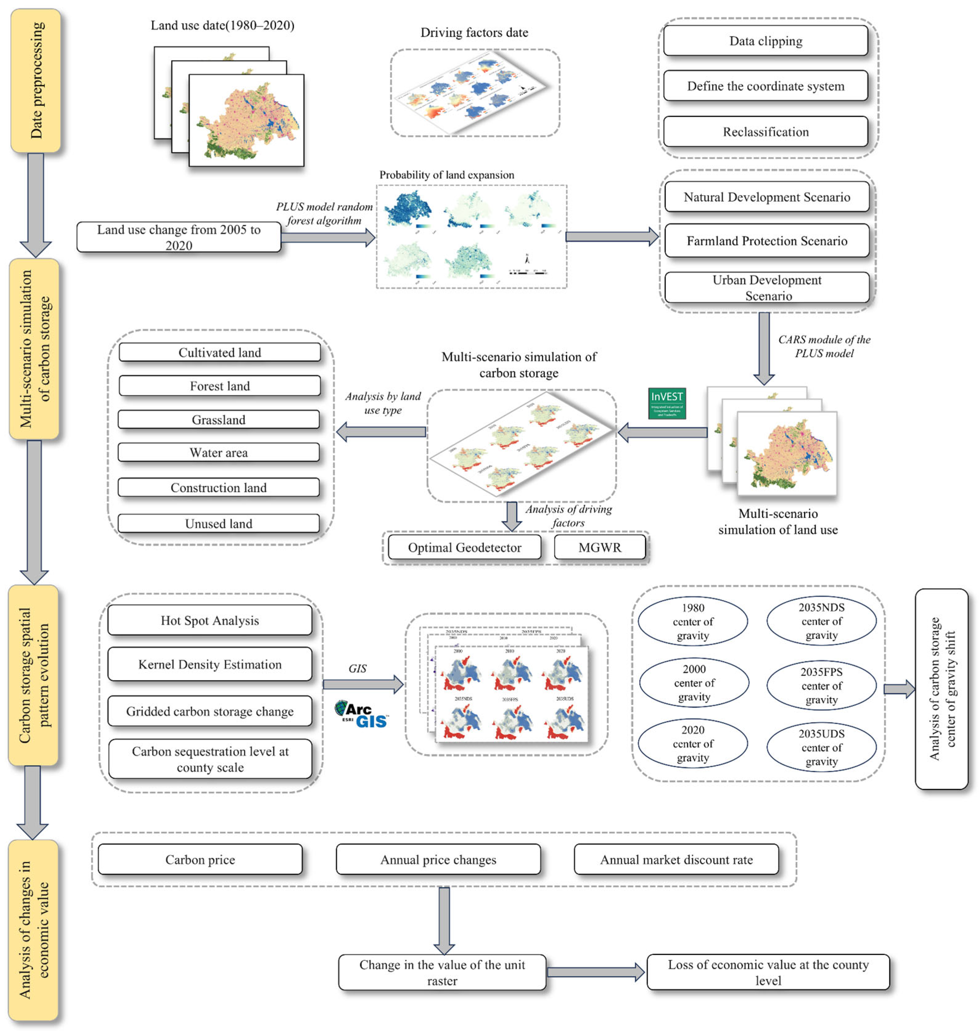
Currently, the aforementioned studies have primarily focused on CS quantification, yet a critical research gap remains regarding the economic valuation of CS loss. To address this knowledge gap, this study establishes an integrated analytical framework encompassing scenario simulation, CS assessment, attribution analysis, and economic valuation. Furthermore, a multi-scale analytical approach (city–grid–raster) is employed to investigate the spatial heterogeneity of CS dynamics.

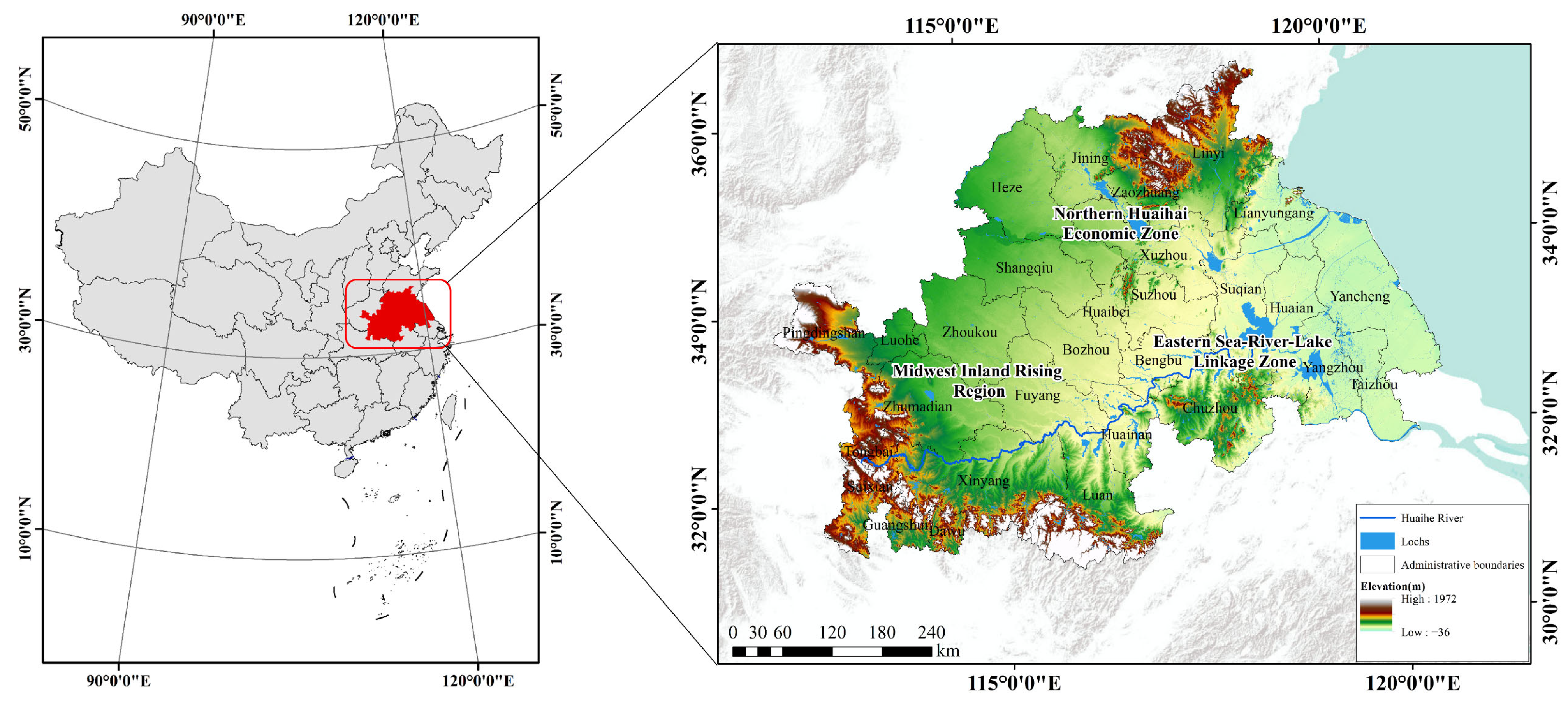
As an important grain-producing area in China, the Huaihe River Basin (HRB) has a large proportion of cultivated land (CUL) and high grain output, along with a substantial CS capacity, thus serving as an important ecological and environmental protection barrier in China [35,36,37]. In this region, consisting of 195 cities, there exists a development imbalance, with eastern cities taking the lead in development over other cities. With the implementation of planning policies, it is inevitable that the development and construction intensity in the region will increase, which poses a risk of CS degradation. Conducting a comprehensive analysis of CS economic value losses under multiple scenarios will provide scientific evidence for land use policy formulation in this region.

The objectives of this study are outlined as follows: (1) to investigate the total quantity and spatial pattern distribution of CS in the HRB during the period from 2000 to 2020 and under multiple scenarios; (2) to examine the driving factors that influence CS; and (3) to explore the alterations in urban-scale CSC and the economic value losses under MSS.

2. Methods

2.1. Study Area

The study area comprises 25 prefecture-level cities and 4 counties, covering a planned territory of 2.43 × 10⁵ km² (Figure 1). This region, with a population of 146 million and 2300 km of navigable waterways, generates a regional GDP of CNY 82.80 trillion. It contributes 1/6 to the national grain production while accounting for 1/4 of the nation’s commercial grain output [21,35,36,37]. The region has a complete transportation infrastructure network, including railways, highways, and waterways, and its energy facilities are continuously upgraded. The region is located in the monsoon climate zone, where the warm-temperate zone transits to the subtropical zone [38]. This region has significant natural ecological advantages. The Huaihe River and its numerous water systems provide abundant freshwater resources and a stable ecosystem. In the western part of the region, there is a high forest coverage. Functionally, this region serves as both a crucial grain production base and a key destination for industrial relocation in China.

2.2. Data Source and Pre-Processing

The main data sources are presented in

Table 1. Data source.

Name	Introduction	Period	Source
Land use data	30 m	1980–2020	https://www.resdc.cn (accessed on 12 March 2025)
Elevation	30 m	2000–2020	https://www.resdc.cn/ (accessed on 12 March 2025)
Average annual temperature	°C	2000–2020	https://www.resdc.cn/ (accessed on 12 March 2025)
GDP per capita	CNY/person	2000–2020	https://www.resdc.cn/ (accessed on 12 March 2025)
Population density	Persons/km2	2000–2020	https://www.worldpop.org/ (accessed on 12 March 2025)
Distance from primary rivers	1 km	2020	https://www.openstreetmap.org/ (accessed on 12 March 2025)
Distance from primary roads	1 km	2020	https://www.openstreetmap.org/ (accessed on 12 March 2025)
Silt content	%	2020	https://gaez.fao.org/pages/hwsd/ (accessed on 12 March 2025)
Clay content	%	2020	https://gaez.fao.org/pages/hwsd/ (accessed on 12 March 2025)
NDVI	0.5°	2020	https://www.resdc.cn/ (accessed on 12 March 2025)

. Among these, the land use data for this study were derived from the land cover remote sensing dataset (CNLUCC) released by the Chinese Academy of Sciences, with a spatial resolution of 30 m × 30 m. The slope was calculated from the elevation date. The driving factors were extracted based on administrative divisions, and the WGS_1984_Albers projection coordinate system was used to ensure uniformity. To enhance the efficiency of software operation, the land use data were resampled to 300 m using the nearest-neighbor method.

2.3. Process Framework

This research mainly goes through four parts and conducts relevant research on CS by coupling multiple models (Figure 2).

2.4. Land Use Transfer Matrix (LUTM)

The LUTM [39] can intuitively reflect the quantity, structure, type, and spatial differentiation of land use. The calculation formula is

$$S_{ij}=\left[\begin{array}{cccc}{S}_{11}& S_{12}& \dots & S_{1n}\\ S_{11}& S_{11}& \dots & S_{2n}\\ \dots & \dots & \dots & \dots \\ S_{n1}& S_{n2}& \dots & S_{nn}\end{array}\right]$$

(1)

where $S$ is the area of a land use type; $n$ is the number of land use types; $i$ is the land use type at the beginning of the study; $j$ is the land use type at the end of the study.

2.5. CS and Net Value Change Assessment Based on the InVEST Model

InVEST is a model system for evaluating the quantity and economic value of ecosystem service functions and supporting ecosystem management and decision-making. It is capable of calculating CS under specific land use conditions and is widely utilized in regional CS assessment. The calculation formula is

$$\begin{array}{l}{C}_t=C_a+C_b+C_s+C_d\\ C_t=\left(C_a+C_b+C_s+C_d\right)\times A_i\end{array}$$

(2)

where $i$ is the average carbon density of each land use type and $A_i$ is the area of land use. Note: $C_a$ is the CS of aboveground organisms; $C_b$ is the CS of underground organisms; $C_s$ is the CS of soil; and $C_d$ is the CS of dead organic matter.

The InVEST valuation module is employed to investigate the alterations in the economic value of CS. Drawing on previous research, it is known that the social cost associated with carbon emissions in China stands at USD 24. Regarding the economic value of carbon sinks, the market discount rate is set at 10%, and the annual variation rate of the social costs for carbon emissions is determined to be 0 [40,41,42].

Carbon density varies according to climate, soil, and land use type and needs to be corrected. This study uses results from relevant scholars [43]. Specific parameters are shown in

Table 2. Carbon density in Huaihe River Basin (unit: T/hm²).

Land Use Type	AbovegroundCarbon Density	UndergroundCarbon Density	Density of SoilCarbon	Carbon Density of Dead Organic Materials
Cultivated land	1.57	0.15	35.1	0
Forest land	8.8	3.17	67.47	0.8
Grassland	0.27	0.69	68.34	0.04
Water area	0.48	0	0	0
Construction land	1.6	0.94	15.92	0
Unused land	1.91	0.31	8.53	0

.

2.6. MSS of Land Use

The PLUS framework functions as a grid-based computational platform specifically designed to simulate land cover dynamics through spatially explicit patch evolution. Its architecture integrates two synergistic components: the LEAS and the CARS. Within the LEAS module, a random forest classifier systematically analyzes the driving factors underlying land use transitions to quantify transition probabilities across heterogeneous landscapes. Concurrently, CARS incorporates spatial proximity effects and stochastic selection mechanisms to resolve inter-category competition, thereby generating multi-scenario land use configurations through iterative optimization. This study referred to the literature of many scholars and set three scenarios based on regional realities [27,44,45,46]. The specific scenario settings and parameter adjustments (

Table 3. Weights in the field of land expansion.

	Cultivated Land	Forest Land	Grassland	Water Area	Construction Land	Unused Land
NDS	0.6	0.1	0.1	0.1	0.7	0.7
FPS	0.4	0.1	0.2	0.1	0.5	0.9
UDS	0.8	0.1	0.3	0.1	0.8	0.5

) are as follows:

(1)

Natural development scenario (NDS): This scenario is based on the land conversion patterns from 2010 to 2020. According to the current development model, no restrictions on land conversion are set and the impact of policy intervention is not considered. The future is predicted and simulated according to the past regular patterns.

(2)

Farmland protection scenario (FPS): High-quality CUL is the lifeblood of a nation. FPS added the concept of CUL protection into NDS. It strictly restricts the expansion of construction land (COL) and gives priority to ensuring the availability of CUL resources. In the scenario setting, the conversion of CUL to other land types is decreased by 30%, and the conversion probabilities among other land types remain unchanged.

(3)

Urban development scenario (UDS): Considering that the HRB is in a strategically important period of development, the urbanization rate of major cities in the region has not yet reached the national average level and has high development potential. With the approval and implementation of relevant policies and planning projects, the region will usher in a period of rapid development. In this scenario, the probability of transforming other lands into COL (excluding forest land) is increased by 30%. The rate of loss of COL will be reduced by 10%. The probabilities of transfer between other land types will remain unchanged.

2.7. Hot Spot Analysis

Hot spot analysis [47] is an effective means to explore local spatial clustering. It can distinguish the degree of the spatial distribution aggregation of variables through hot spots. Its mathematical expression is as follows:

$$G_i^{\ast }={\displaystyle \frac{{\displaystyle \sum _{j=1}^n{W}_{ij}{X}_j-\overline{X}{\displaystyle \sum _{j=1}^{\mathrm{n}}{W}_{ij}}}}{S\sqrt{\frac{n{\displaystyle \sum _{j=1}^n{W}_{ij}^2-{\left({\displaystyle \sum _{j=1}^n{W}_{ij}}\right)}^2}}{n-1}}}}$$

(3)

where $X_j$ is the observed value of region $j$; $W_{ij}$ represents the spatial weight matrix; $n$ represents the number of studies; $\overline{X}$ is the average value of all regional observations; and $S$ is the standard deviation.

2.8. Standard Deviational Ellipse (SDE) and Center of Gravity Distribution

SDE [48] is a method in spatial statistics that can accurately reveal the multi-faceted characteristics of the distribution of samples. It is used to reveal the spatial distribution characteristics of geographic elements. The core formula of SDE is as follows:

$$\Sigma =\left(\begin{array}{cc}Var(x)& \mathrm{cov}(x,y)\\ \mathrm{cov}(x,y)& Var(y)\end{array}\right)$$

(4)

where $Var(x)$ and $Var(y)$ represent the variance of the data in the $x$ and $y$ directions, reflecting the degree of dispersion of the data. $\mathrm{cov}(x,y)$ represents the covariance of $x$ and $y$.

The center of gravity distribution [49] is used to analyze the movement trend of geographic features in space. Its formula is

$$\overline{X}={\displaystyle \frac{{{\displaystyle \sum }}_{i=1}^n{w}_i{x}_i}{{{\displaystyle \sum }}_{i=1}^n{w}_i}},\hspace{1em}\overline{Y}={\displaystyle \frac{{{\displaystyle \sum }}_{i=1}^n{w}_i{y}_i}{{{\displaystyle \sum }}_{i=1}^n{w}_i}}$$

(5)

where ($x_i{y}_i$) is the coordinate of the i-th geographic unit, and $x_i{y}_i$ is the weight. By comparing the centroid positions at different time points, the migration direction and intensity of the spatial distribution can be analyzed.

2.9. Optimal Geodetector

The Geodetector is a tool for detecting the driving mechanism of factors. On this basis, the OPGD searches for the optimal natural breakpoint method to find the best breakpoint.

2.10. Multi-Scale Geographically Weighted Regression

The MGWR model reveals the changing relationship of various influencing factors at different geographical locations and scales by setting different neighborhoods (bandwidths) for each explanatory variable and accurately analyzing their spatial heterogeneity. The formula is as follows:

$$Y_i={\beta }_0\left(u_i,v_i\right)+{\displaystyle \sum }_{j=1}^p{\beta }_j\left(u_i,v_i\right)X_{ij}+{\epsilon }_i$$

(6)

where $Y_i$ represents the observed value of the dependent variable at the $\left(u_i,v_i\right)$ geographical location. ${\beta }_0$ is a constant term related to the geographical location. It changes with the geographical location and reflects the baseline level of the dependent variable at different locations. $p$ represents the number of explanatory variables. ${\beta }_j$ is the coefficient associated with the j-th explanatory variable. $X_{ij}$ is the value of the i-th explanatory variable at the j-th observation point. ${\epsilon }_i$ represents the unexplained part of the model and the measurement error.

3. Results

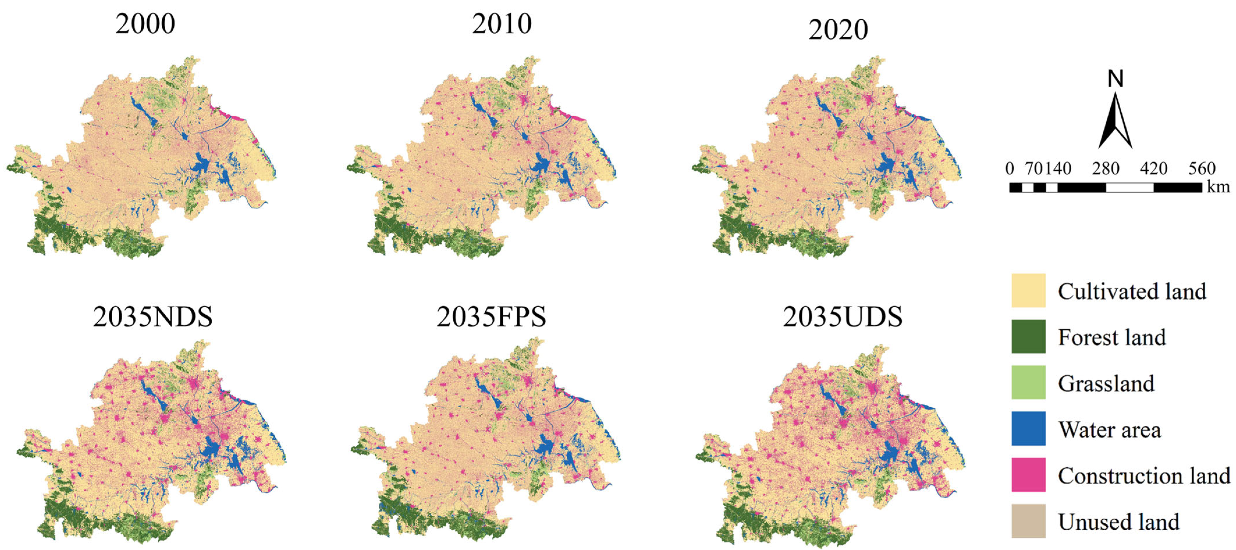
3.1. LUCC Changes from 2000 to 2020

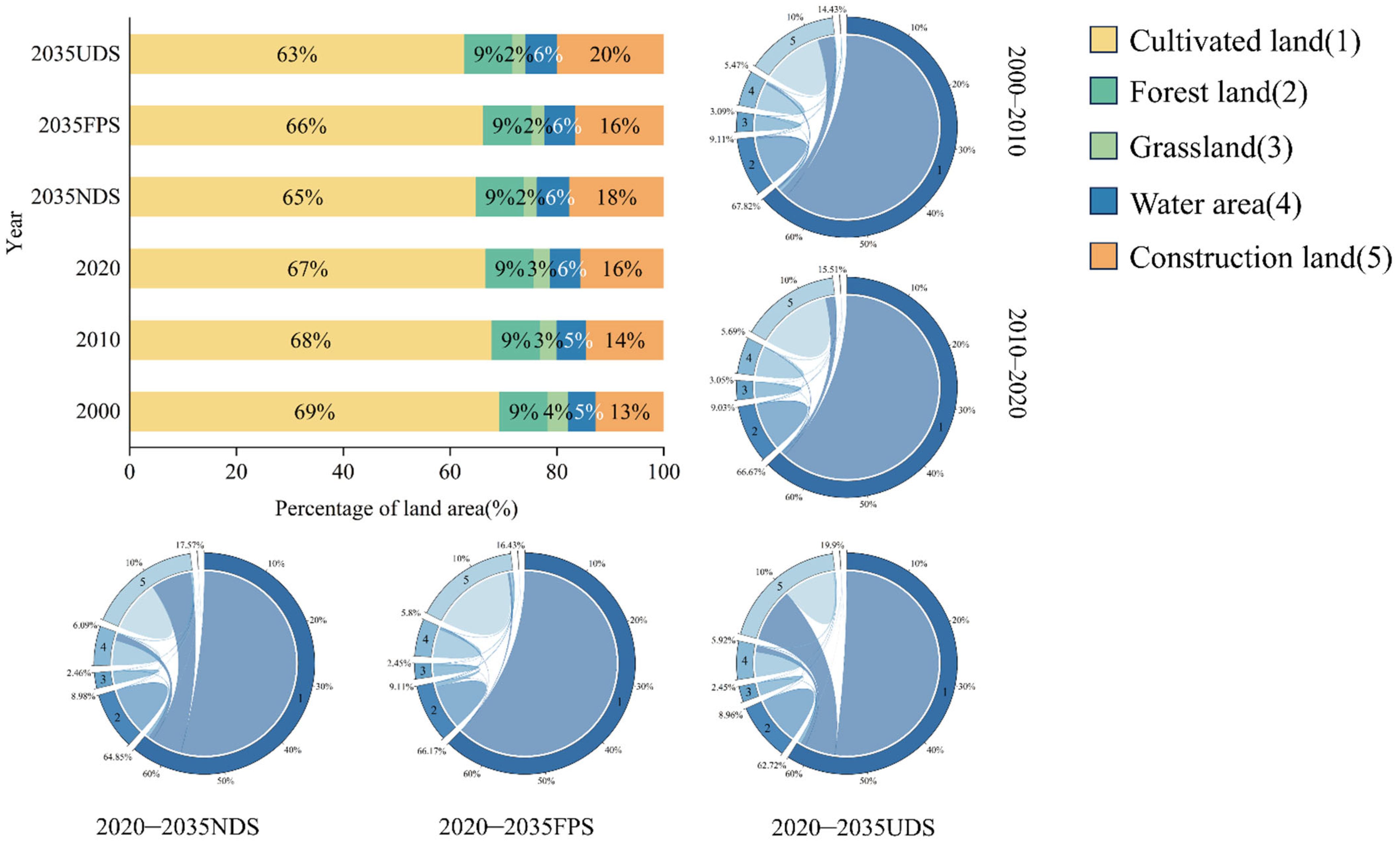
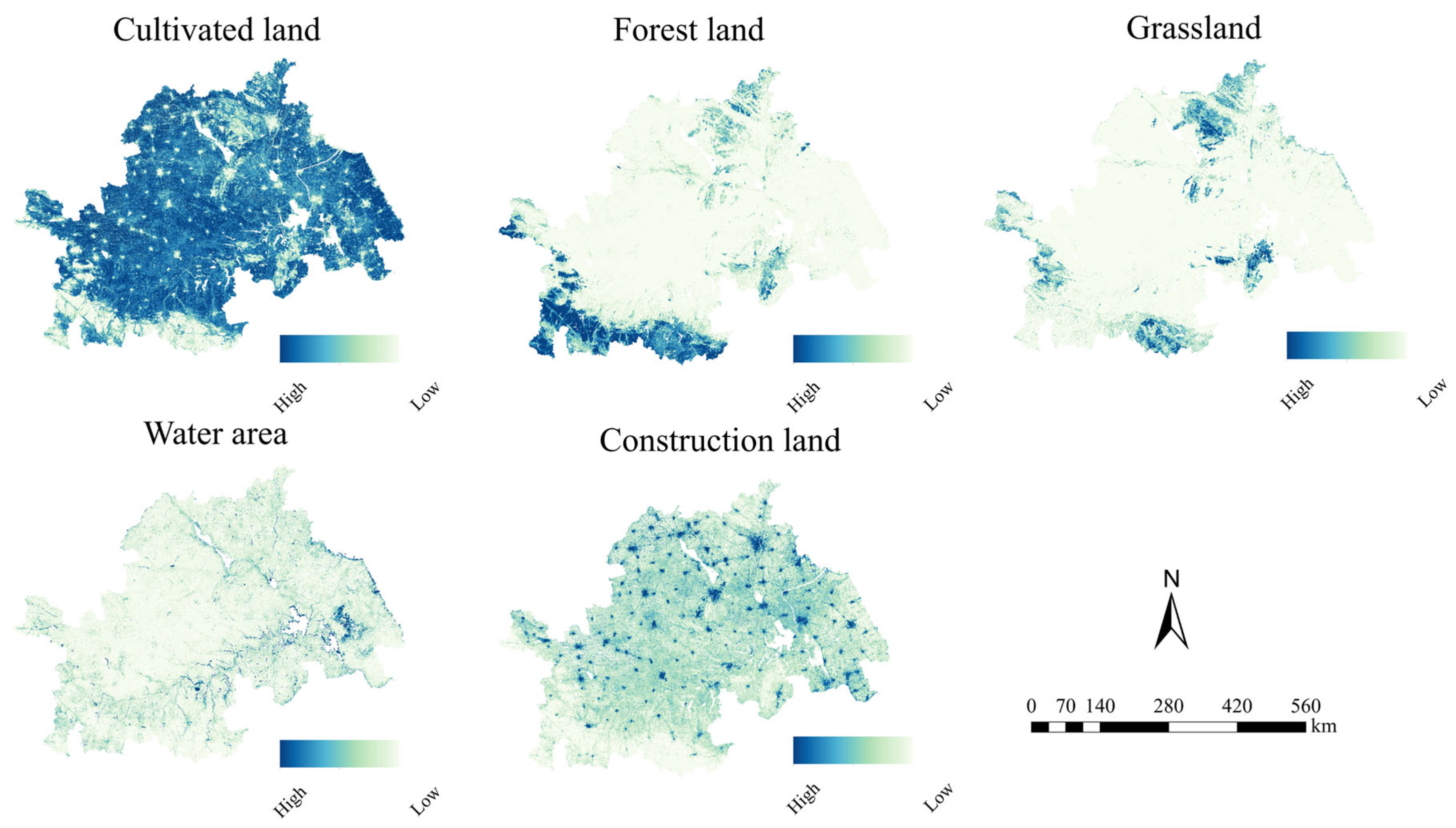
The land use structure exhibits a remarkable dual-dominant feature. CUL and COL prevailed during the period from 2000 to 2020, and both invariably accounted for over 80% of the total area (Figure 3 and Figure 4). The evolution trends of the two showed obvious differences: the CUL area continued to shrink, with a net decrease of 6710 km², a decrease of 3.7%. On the other hand, the COL expanded rapidly, with a net increase of 7551 km², an increase of 22.9%, which constituted the core contradiction of regional LUCC.

Other land types exhibited differentiated change characteristics: forest land had slight fluctuations (+124 km²), water areas expanded significantly (+1494 km²), and unused land decreased slightly (−31 km²). It is worth noting that the grassland area decreased rapidly (−2114 km²), and its change magnitude ranked first in negative changes. This is mainly attributed to the relatively low ecological and economic value of grassland, which was largely developed and converted into construction or agricultural space during the urbanization process. The cumulative land conversion area during the study period reached 24,644 km², accounting for 10.4% of the total area. The CUL-COL conversion process was particularly prominent, with the scale of conversion reaching 11,794 km², accounting for 47.9% of the total conversion volume.

The temporal analysis reveals that the period from 2000 to 2010 witnessed dramatic transformations, exhibiting an average annual change intensity of 1819.6 km²/year (cumulatively 18,196 km², representing 7.5% of the total area). This magnitude markedly exceeds the subsequent decade’s rate of 949 km²/year (2010–2020; cumulatively 9485 km², accounting for 3.6%), demonstrating distinct phase characteristics in the urbanization process.

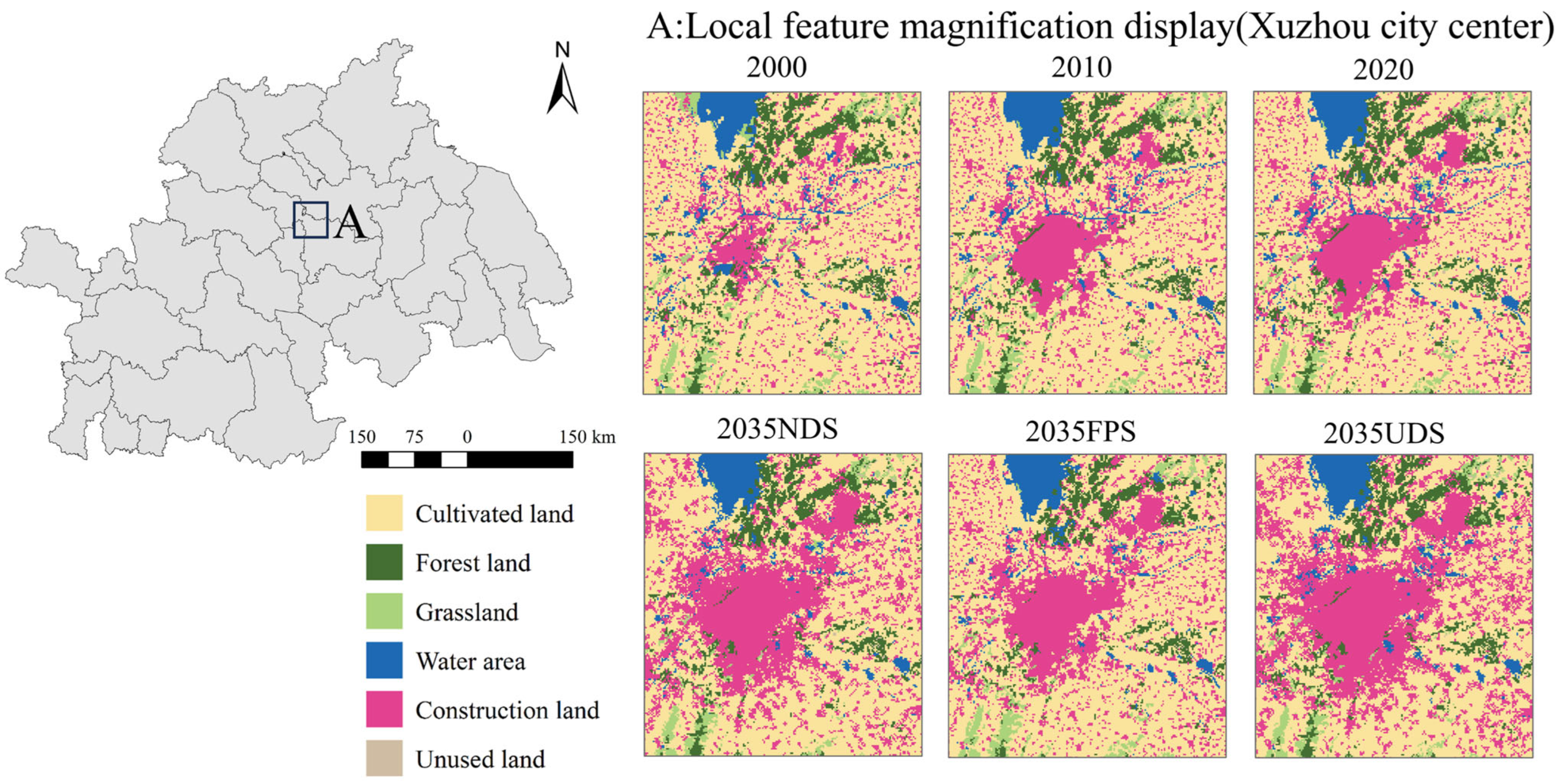
3.2. LUCC of MSS

The land use in 2020 was simulated by means of the transformation relationship from 2000 to 2010. The validation results yielded a Kappa coefficient of 0.83 and an overall accuracy of 0.92, indicating excellent predictive performance. The LEAS module of the PLUS model employs the machine learning random forest algorithm to calculate the probability of land expansion while taking into account the selected driving factors. The results indicate that, on the whole, arable land has the greatest likelihood of expansion. COL comes next in terms of expansion probability. Furthermore, regions with elevated probabilities of forest and grassland expansion are predominantly located in the southwestern study area (Figure 5).

Through the simulation and analysis of the three scenarios (compared with the base year of 2020), the research area exhibits the following common evolution patterns: the area of CUL is undergoing a decreasing trend, while the area of COL keeps increasing. In terms of the overall transfer rate of CUL to COL, there are certain differences among the different scenarios, specifically ranked as 2035UDS > 2035NDS > 2035FPS. These results suggest that the conversion rate of CUL to COL is the fastest under 2035UDS, and 2035FPS inhibits this transformation to a certain extent (Figure 6).

In addition to CUL and COL, other land types also exhibit their own change characteristics under the three scenarios. The grassland area shows varying degrees of reduction across all scenarios, whereas the water area exhibits a moderate increase, primarily attributed to water conservancy infrastructure development and improved water resource management. The spatial distribution pattern of forest land in the HRB is relatively stable, and its change rate does not exceed 1% in the simulations of the three scenarios. For instance, the overall pattern of the Dabie Mountain Ecological Protection Area in the southwest and the Shandong Hills in the northwest has remained basically unchanged. Meanwhile, the changes in the basin area of the mainstream HRB and lakes such as Hongze Lake, Luoma Lake, and Gaoyou Lake are relatively small. All these situations indicate that the overall ecological protection pattern in the HRB is favorable, and the ecosystem has a certain degree of stability and anti-interference ability.

Compared with the NDS, the UDS emphasizes the continuous promotion of urbanization. In the UDS, the probability of other land types being converted into COL is elevated, while the probability of existing construction land being transformed into other land uses is reduced. Under this precondition, from the corresponding time node, the area of COL is 6087 km² larger than that in the NDS. On the other hand, the CUL area is decreased by 5582 km² (

Table 4. LUCC status in different periods (unit: km²).

	Cultivated Land	Forest Land	Grassland	Water Area	Construction Land	Unused Land
2000	180,844	23,713	10,078	13,384	32,965	193
2010	177,119	23,791	8058	14,299	37,690	254
2020	174,134	23,589	7964	14,879	40,516	162
2035NDS	169,426	23,447	6427	15,907	45,893	143
2035FPS	172,854	23,788	6395	15,149	42,921	136
2035UDS	163,844	23,417	6401	15,462	51,980	139

). This indicates that while the UDS promotes the urbanization process, it may impose a certain pressure on CUL resources.

Compared with the NDS, the FPS plays a crucial role in the protection and high-quality development of CUL. By 2035, under the FPS, the CUL area will be 3428 km² more than that in the NDS, while the area of COL will be reduced by 2972 km². This fully illustrates the effects of the FPS in protecting cultivated land resources.

3.3. Changes in CS

3.3.1. CS Change in 2000–2020

CS from 2000 to 2020 has generally exhibited the characteristics of phased decline (Figure 7,

Table 5. CS in different land types (unit: T).

	Cultivated Land (×108)	Forest Land (×108)	Grassland (×107)	Water Area (×105)	Construction Land (×107)	Unused Land (×105)	Total (×108)
2000	6.66	1.90	6.99	6.42	6.09	2.08	9.88
2010	6.52	1.91	5.59	6.86	6.96	2.73	9.69
2020	6.41	1.89	5.52	7.14	7.48	1.75	9.61
2035NDS	6.24	1.88	4.46	7.64	8.47	1.54	9.42
2035FPS	6.36	1.91	4.43	7.27	7.92	1.47	9.52
2035UDS	6.03	1.88	4.44	7.42	9.60	1.50	9.32

), with CS in 2000 > CS in 2010 > CS in 2020, and with a total reduction of 2.64 × 10⁷ T in 20 years. The decline during 2000–2010 was greater than that during 2010–2020. Specifically, the decrease during 2000–2010 was 1.8%, representing a decrease of 1.83 × 10⁷ T, while the decrease in CS during 2010–2020 was 0.8%, with a decrease of 8.12 × 10⁶ T.

As the predominant carbon pools, CUL and forest land account for more than 86% of CS, constituting the regional carbon sink base. In contrast, water bodies and unused land exhibit limited carbon sequestration capacity, each contributing less than 1%, highlighting the marginal role of these land types in the carbon cycle.

The carbon pool loss of CUL (−2.47 × 10⁷ T) and the carbon pool gain of COL (+1.39 × 10⁷ T) form the main carbon flux, reflecting the dominant mechanism of “CUL-COL” transformation during the rapid urbanization process. The grassland CS has dropped sharply by 20.8%, showing its sensitivity as a fragile ecosystem. The CS of COL has increased by 22.9%, indicating that human activities have led to the transformation of some land carbon sink functions.

3.3.2. Changes in CS Under MSS

The carbon–land association mechanism exhibits a significant linear response characteristic. There are gradient differences in the carbon sequestration efficiency per unit area (forest land > grassland > cultivated land > construction land > unused land > water area), which verifies that land use type is a crucial factor in regulating the efficiency of carbon sinks.

The changes in CS simulated by MSS display different policy sensitivities (Table 5). Taking the 2035NDS as the benchmark, the 2035FPS increases CS by 1.2% (+1.53 × 10⁶ T) through the implementation of high-standard farmland construction, while the UDS leads to a 2% decrease in CS (−2.64 × 10⁶ T) because of the expansion of COL. The CS of the three scenarios is ranked as FPS (7.68 × 10⁷ T) > NDS (7.59 × 10⁷ T) > UDS (7.44 × 10⁷ T), emphasizing the regulatory potential of territorial spatial planning on the carbon balance. Compared with the base year of 2020, the area of CUL in 2035 will be reduced under the three scenarios, and the COL will keep expanding. In the FPS, a net increase of 3428 km² in the CUL area and an increase of 1.26 × 10⁷ T in the carbon sink were achieved through the strategy of improving the CUL quality. In the UDS, the carbon sink effect on the site is enhanced (+1.12 × 10⁷ T) due to a sharp increase of 6087 km² in the COL.

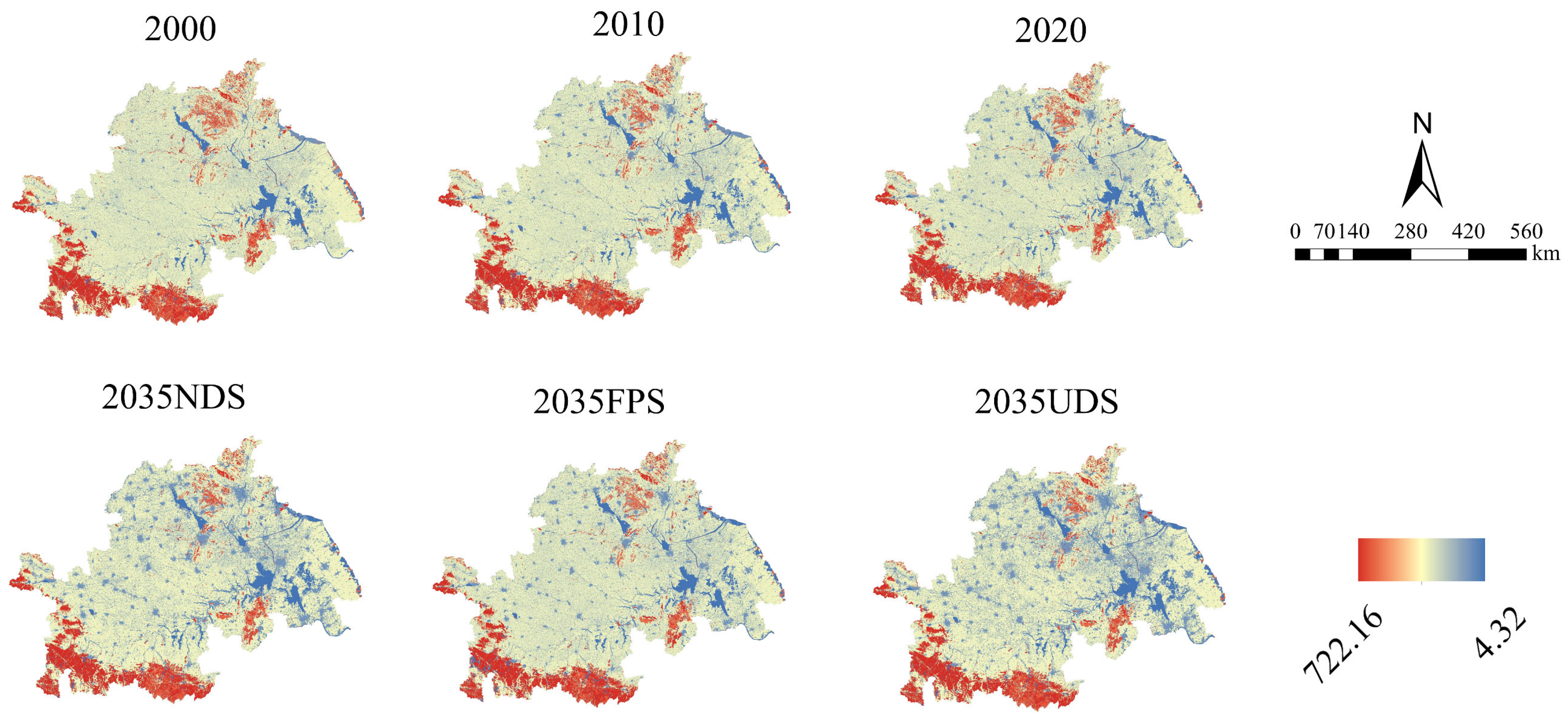
3.3.3. CS Spatial Differentiation from the “City–Grid–Raster” Perspective

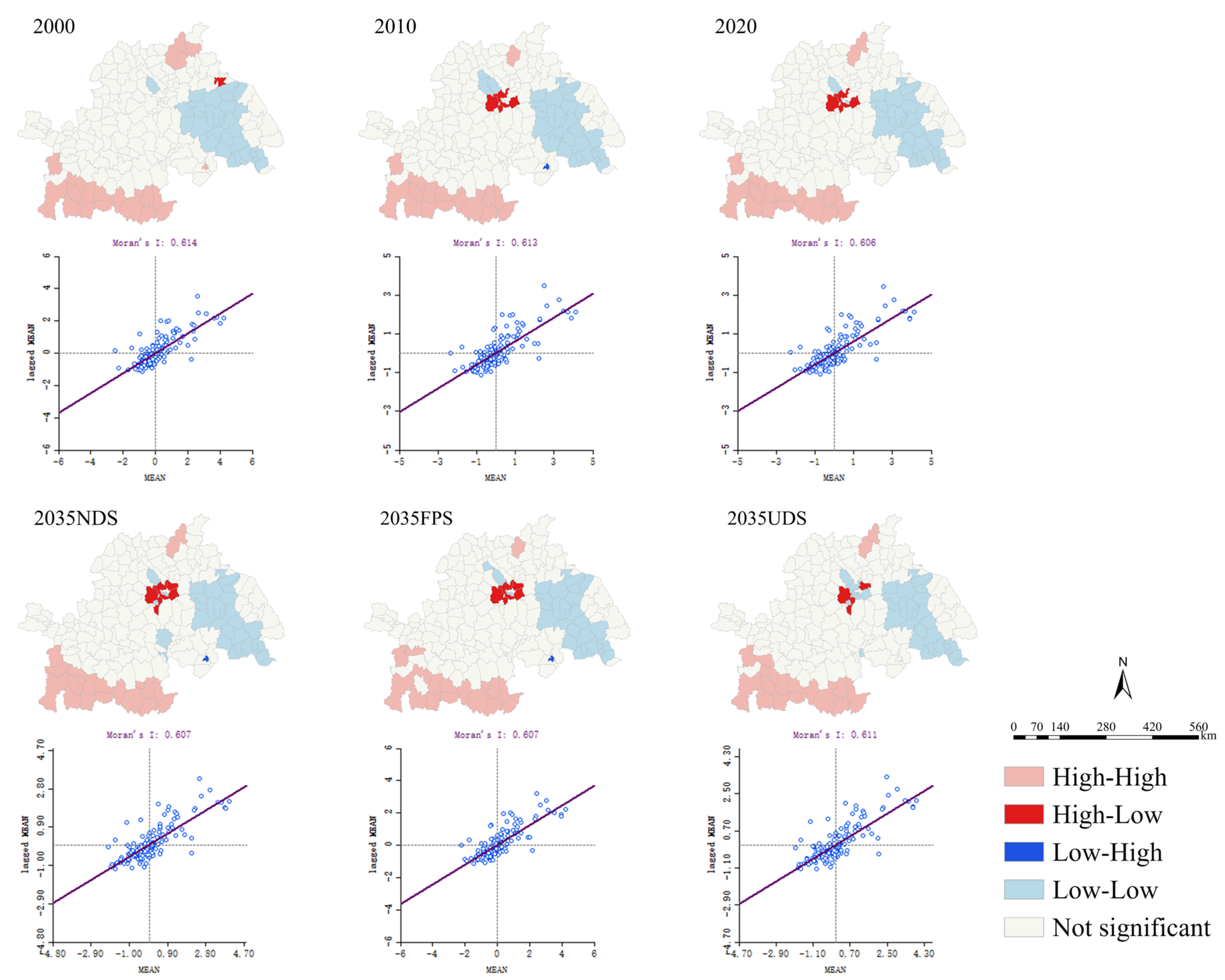
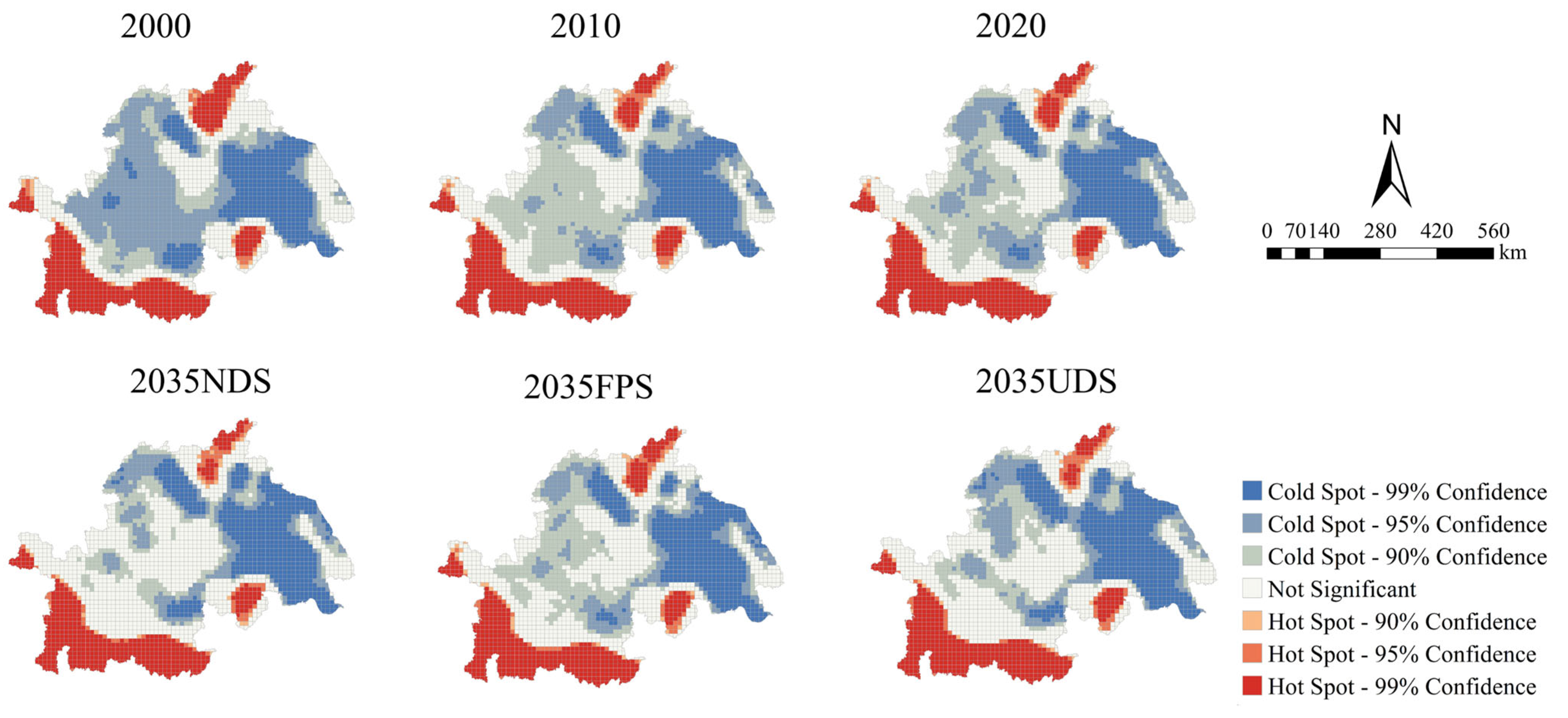
At the city scale, Moran’s I values in all six periods are greater than 0.6, which indicates significant spatial autocorrelation. Among them, the cities in the southwestern region show a continuous high–high agglomeration trend, the eastern region shows a continuous low–low agglomeration, and the central region shows a high–low agglomeration trend (Figure 8).

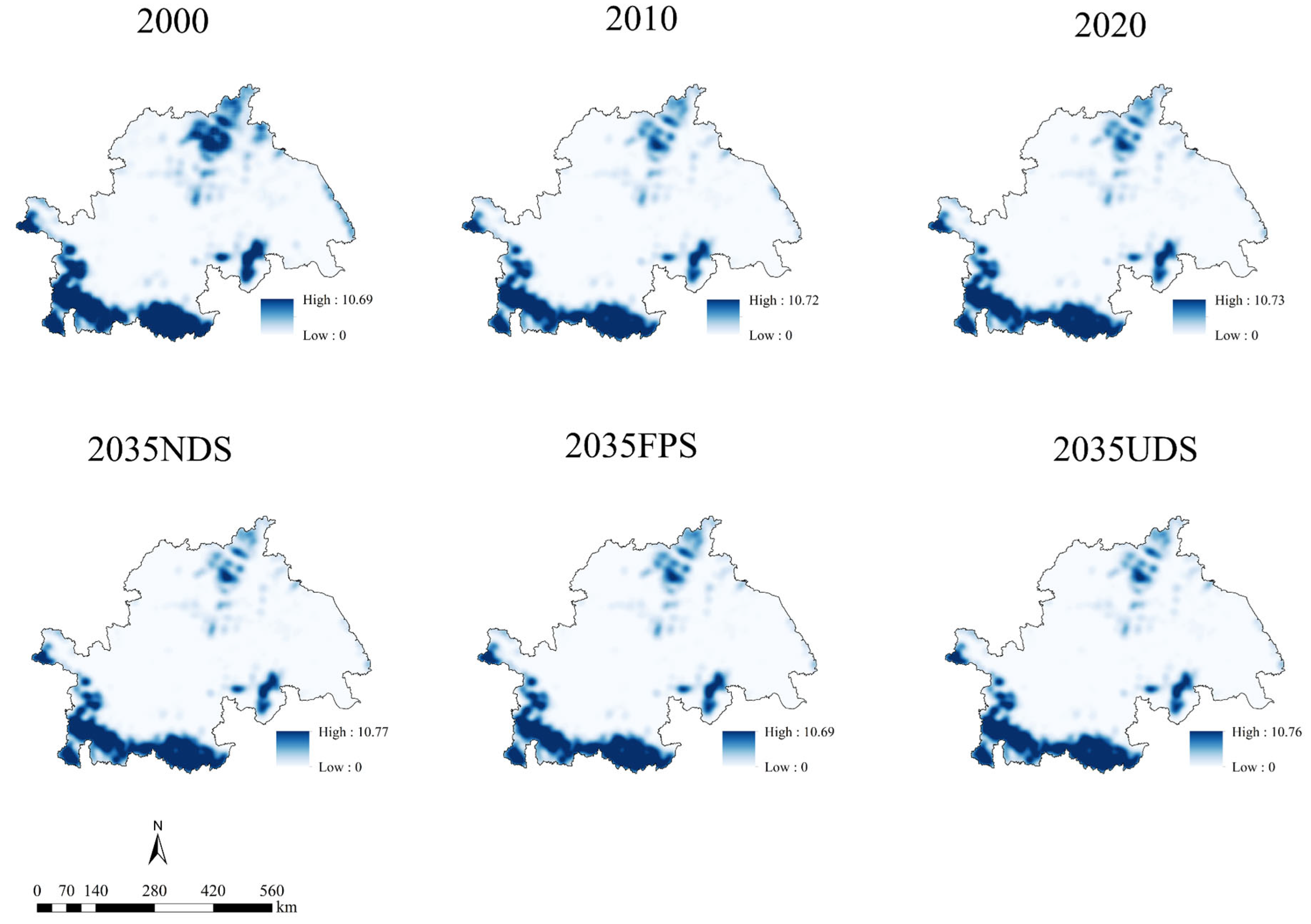
At the grid and raster scales, the distribution of CS shows significant spatial heterogeneity (Figure 9 and Figure 10). The spatial pattern of hot and cold spots is stable; however, there are temporal differences in the agglomeration intensity. High-value hot spots are distributed in three major ecological barrier areas: the Dabie Mountain tectonic belt in the southwest (including the extension area of the Tongbai Mountain), the mountainous and hilly areas in central and southern Shandong in the north, and the Zhangbaling low mountains and hills in Chuzhou. The low-value cold-spot area shows the characteristics of “agglomeration around the lake” and is mainly distributed around large water bodies such as Gaoyou Lake and Yunlong Lake.

The area of hot spots has shown a significant reduction trend from 2000 to 2020, from 57,571 km² (22%) to 54,890 km² (21%) in 2020. In the MSS, 2035FPS > 2035NDS > 2035UDS, but none of them are as large as the 2020 hot spot area (

Table 6. Extreme hot spot area (unit: km²).

	2000	2010	2020	2035NDS	2035FPS	2035UDS
Extremely hot spot area	57,571	55,820	55,433	54,388	55,299	53,720

).

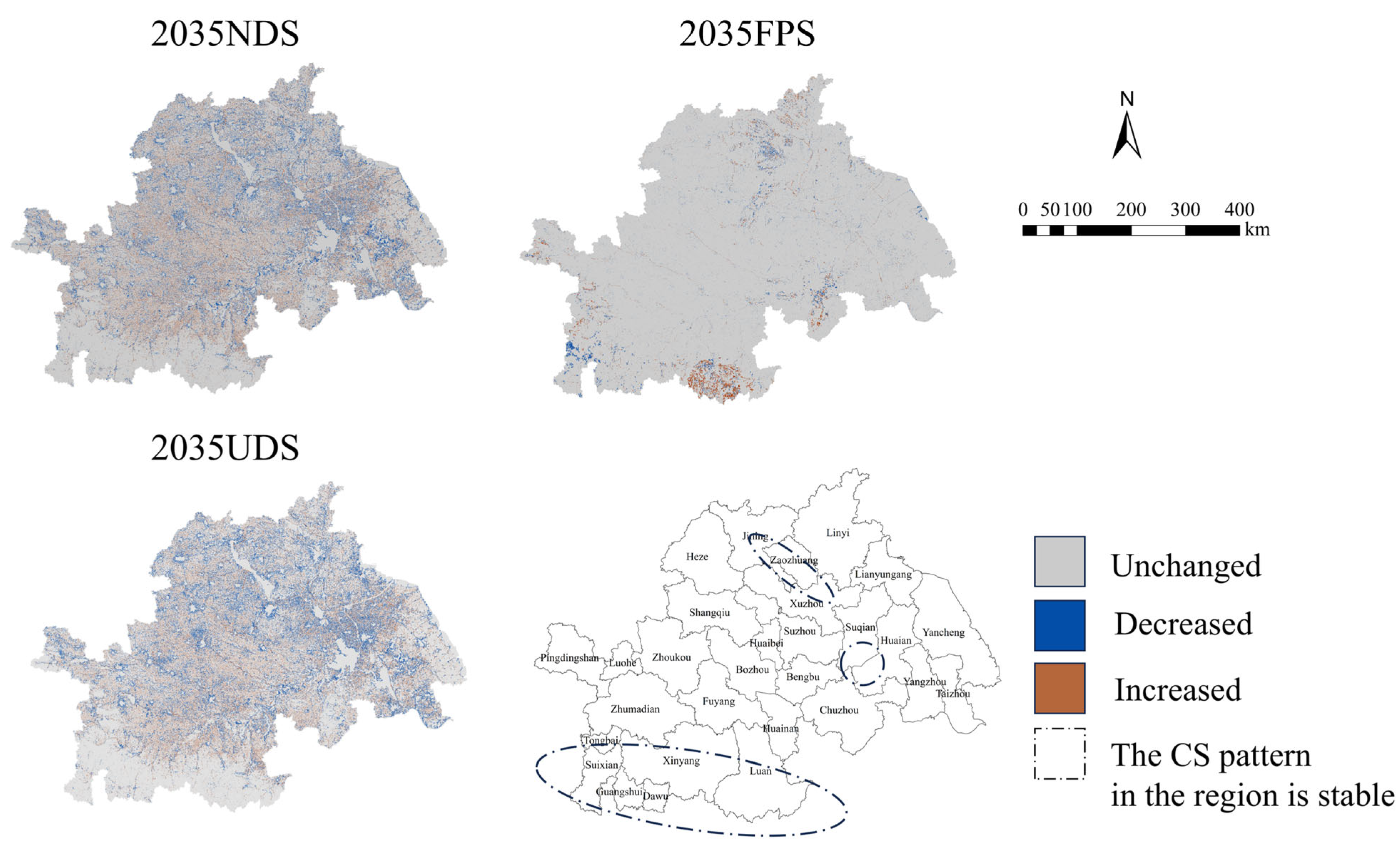
In the three scenarios, the base year of 2020 indicates that the number of grids with a decrease in CS is larger than that with an increase in CS. The number of reductions follows the order of 2035UDS > 2035NDS > 2035FPS, and overall, 2035FPS has the least change. Among the three scenarios, there are three major regions with minimal changes, suggesting that the overall spatial pattern in the southwest region and around lakes is stable (Figure 11).

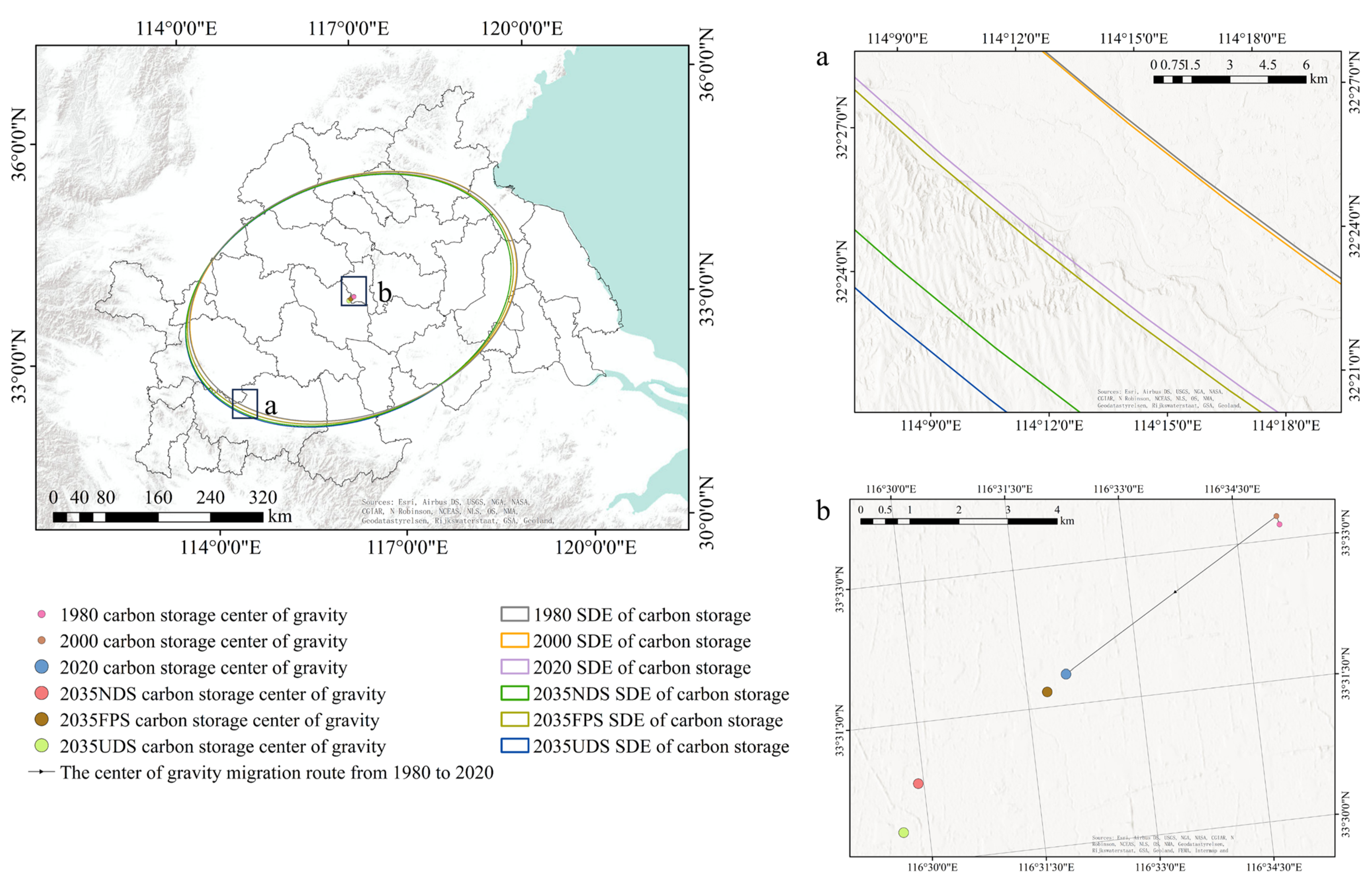
3.4. Analysis of CS Center of Gravity Shift

Based on the CSC of each municipal administrative unit, both the standard deviation ellipse (SDE) and the center of gravity distribution (CGD) indicate that the overall carbon sequestration pattern migrated towards the southwest between 1980 and 2020. The migration speed from 2000 to 2020 was higher than that from 1980 to 2000. Under the three forecast scenarios, the trajectory of the CGD continued to shift southwestward compared to 2020, with the UDS migration rate > NDS migration rate > FPS migration rate (Figure 12,

Table 7. Center of gravity coordinates.

	1980	2000	2020	2035NDS	2035FPS	2035UDS
Longitude	116°35′5.17″ E	116°35′3.45″ E	116°32′2.47″ E	116°29′55.58″ E	116°31′46.02″ E	116°29′39.50″ E
Latitude	33°33′9.57″ N	33°33′15.62″ N	33°31′49.84″ N	33°30′50.80″ N	33°31′39.89″ N	33°30′20.52″ N

). The primary reason for this migration is that land change in the southwest is relatively minor, the intensity of human activity is low, the overall forest pattern remains favorable, and the CSC remains stable. However, apart from the southwest region, urbanization in other regions has accelerated, and a large amount of land has been converted from CUL to COL, resulting in a decline in the overall CSC, which is manifested as the continuous movement of the center of gravity towards the southwest, reflecting the decline in the overall CSC of the region.

3.5. Analysis of Driving Factors

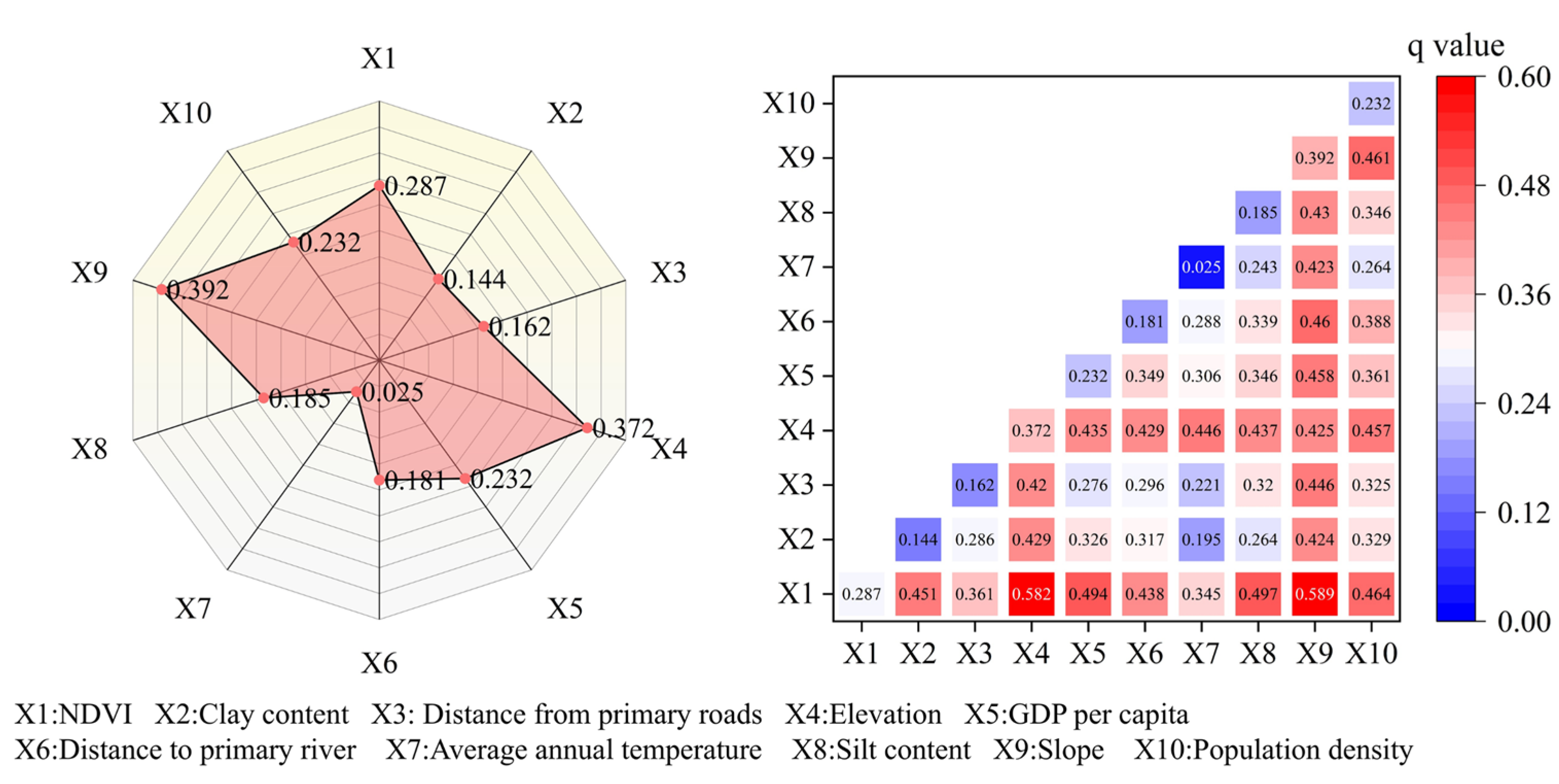
Based on relevant literature, ten driving factors were selected from multiple levels for analysis. All relevant data were masked in the GIS and matched with administrative regions, and then the grid factor data were discretized. The classified CS density was taken as the Y-value. The OPGD was utilized to conduct the best natural breakpoint iteration for grouping the interactive detection module and factor detection module to explore the interaction and single-factor influence among driving factors. For cities and counties, the CSC of each county-level administrative area was regarded as the dependent variable to explore the spatial heterogeneity of the driving factors. All operation results met the training accuracy requirements. The results are as follows:

The top five driving factors are elevation, slope, NDVI, GDP per capita, and population density, accounting for 77.2% of the total driving force. This shows that topographic natural factors and socio-economic factors significantly affect the regional CSC.

The interaction detection module shows that the interaction is of two types—dual-factor enhancement and nonlinear enhancement—indicating that the coupling driving effect of dual factors is stronger than that of single factors. Among them, the main mode of interaction between average temperature and other factors is dual-factor enhancement (Figure 13).

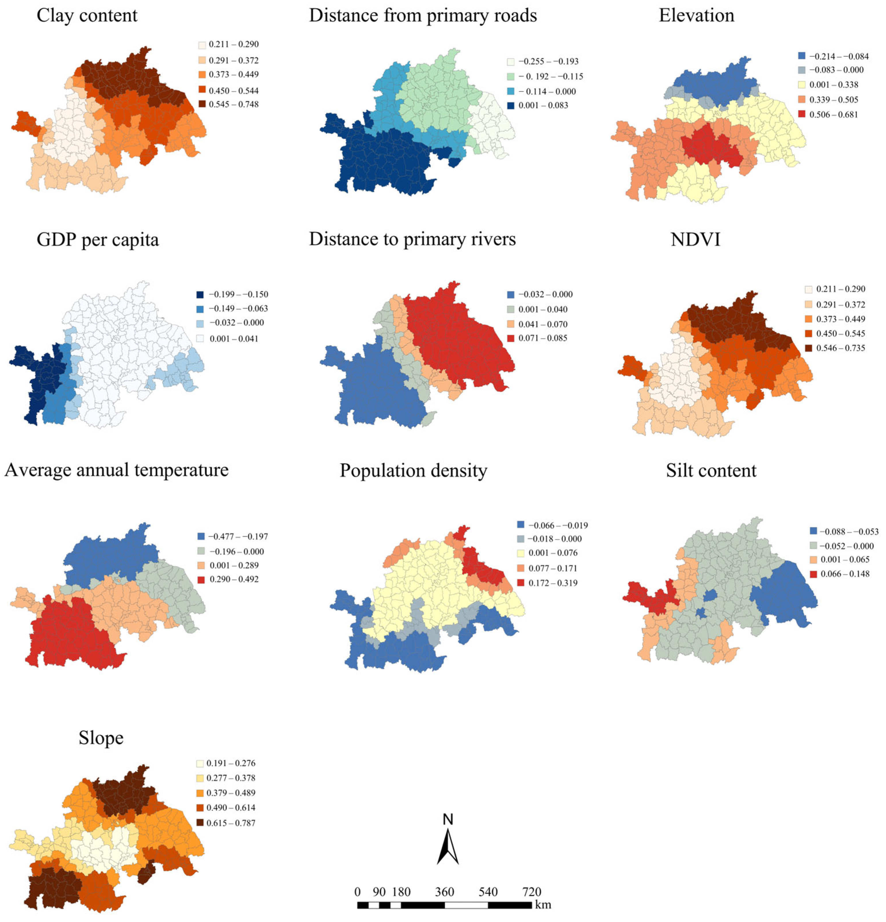
Analysis of the three models (OLS, MGR, MGWR) indicated that MGWR had the largest adjusted R², the smallest AICc, and the highest model fit and accuracy (

Table 8. Model accuracy comparison.

	R2	Adjusted R2	AICc
OLS	0.72	0.78	366.72
MGR	0.79	0.84	288.73
MGWR	0.82	0.88	236.54

). The results demonstrated the following (Figure 14): (1) The distribution of CS is influenced by the coupling of multiple factors and exhibits significant scale dependence, while the spatial heterogeneity of different factors varies considerably. Globally, slope, clay content, and NDVI have a significant positive impact. (2) The correlations between factors such as the distance from primary roads, average temperature, and CS vary between positive and negative in different regions, reflecting the complex impacts of these factors on CS.

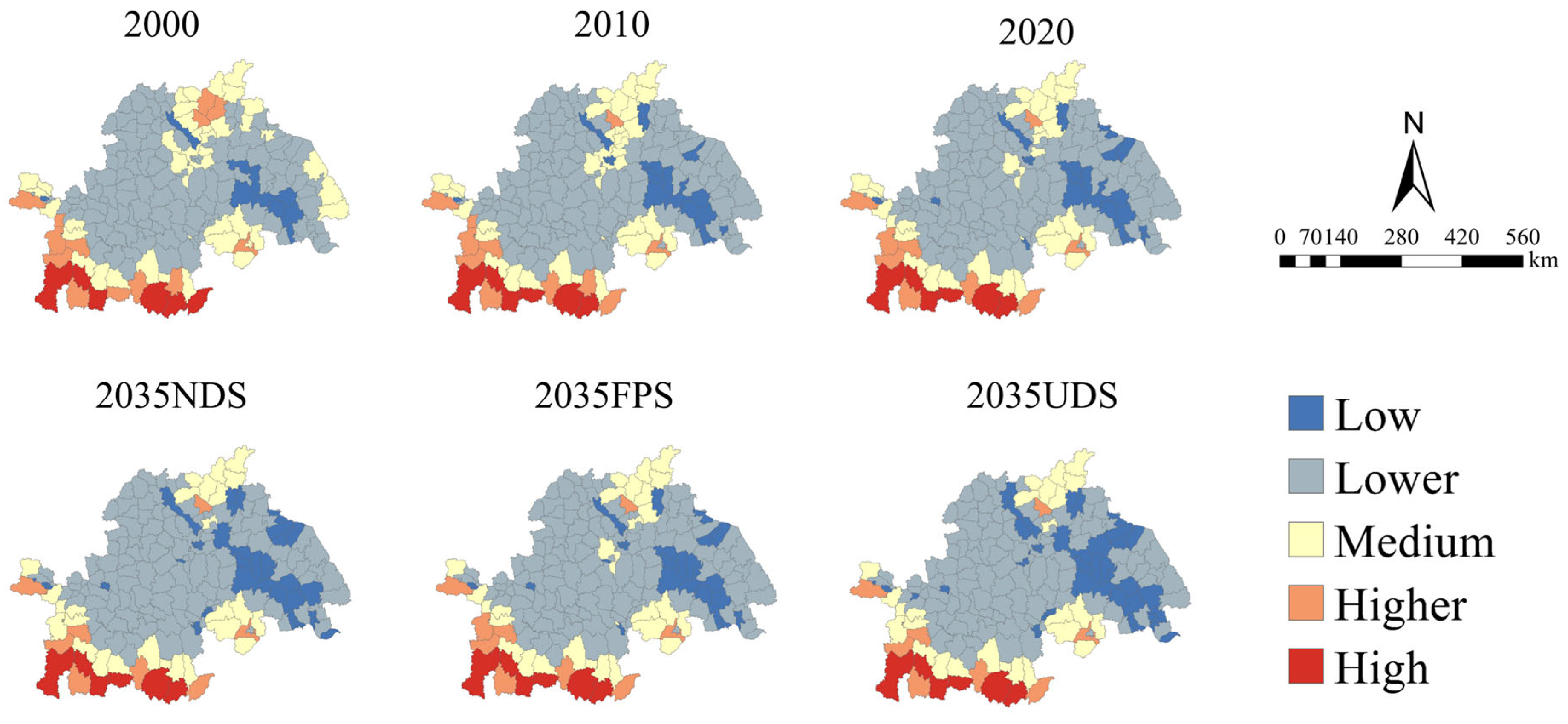
3.6. Changes in CSC at the City Level

This study assessed the regional CSC in light of the average CS per unit grid and classified it into five levels by means of the Jenks package in the R language (Figure 15,

Table 9. Level changes.

	I	II	III	IV	V	Number of Changes
2000	10	125	41	12	7	/
2010	20	124	34	11	6	23
2020	26	121	33	9	6	11
2035NDS	38	117	26	8	6	19
2035FPS	28	123	29	9	6	4
2035UDS	45	110	26	8	6	28

Note: The changes are relative to the previous period.

). Time-series analysis indicated that during 2000–2020, the spatial differentiation of carbon sequestration capacity exhibited a distinct gradient feature: the central and western inland rising areas > the northern Huaihai Economic Zone > the eastern Haihe River-Lake Linkage Area. Among them, the southwestern region maintained a strong carbon sequestration capacity, while the eastern coastal areas remained at a low level continuously.

Between 2000 and 2020, the CSC level of all city-level administrative units did not decline by more than one level, and no significant degradation took place. Observations by time period indicated that the CSC changed significantly from 2000 to 2010, with a total of 23 administrative units undergoing a one-level drop (mainly distributed in the northern and eastern coastal areas); the rate of change decelerated from 2010 to 2020, with only 11 administrative units having a level drop.

In the MSS, the influence of different scenarios on the change in CS in counties and cities follows the order of 2035UDS > 2035NDS > 2035FPS. Specifically, under the 2035NDS, a total of 19 boroughs will experience a one-level reduction in their CSC levels, and under the 2035UDS, a total of 28 city-level administrative regions will experience a one-level reduction in their CSC levels; however, under the 2035FPS, only 4 county-level regions will experience a one-level reduction in their CSC levels, which is basically the same as the carbon sequestration grade pattern in 2020.

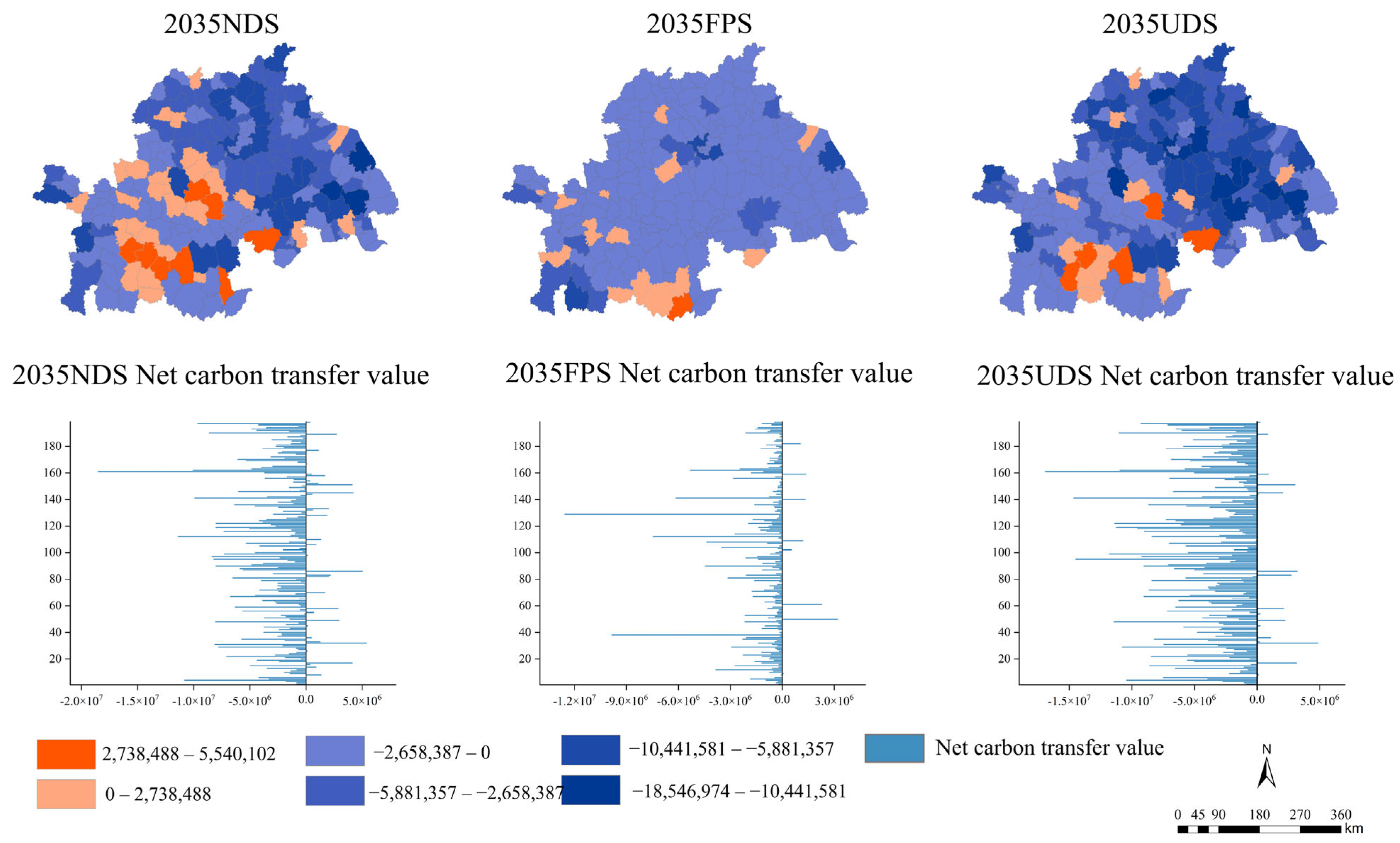
3.7. Changes in the Economic Value of CS Under MSS

Under MSS, CS decreased to varying degrees, with the degree of reduction following the order 2035UDS > 2035NDS > 2035FPS (Figure 16), and the resulting carbon economic losses were USD 6.90 × 10⁸, 4.57 × 10⁸, and 2.28 × 10⁸, respectively. At the county level, most of the carbon economic value was lost, with the number of cities with economic loss following the order 2035FPS > 2035UDS > 2035NDS, but the average loss followed 2035FPS < 2035NDS < 2035UDS (

Table 10. Loss of economic value.

	2020–2035NDS	2020–2035FPS	2020–2035UDS
Number of cities with net value increase	34	16	18
Number of cities with net value reduction	161	179	177
Loss of CS (T)	1.92 × 107	9.57 × 107	2.89 × 107
Loss of economic value (USD)	4.57 × 108	2.28 × 108	6.90 × 108

).

Overall, the eastern and northern regions have a greater risk of CS loss and a faster rate of economic loss. It is worth noting that high-intensity urbanization has a substantial negative effect on the regional carbon sink function. The ecological compensation costs it causes may increase the local fiscal burden and there is a systemic risk of triggering a chain reaction of local fiscal risks.

4. Discussion

4.1. Interrelationships Between Driving Factors and Land Use Patterns

The driving mechanisms of CS are complex, involving the coupled effects of multiple factors. This study attempts to analyze 10 selected factors across multiple dimensions to identify those with significant impacts on CS distribution and quantify their contribution values. Altitude, slope, NDVI, GDP per capita, and population density collectively account for 77.2% of the total driving forces, indicating that both natural factors and human activity intensity are key determinants of CS variations. Specifically, high values of DEM, slope, and NDVI are predominantly observed in the southwestern Dabie Mountain region, where CS levels are elevated and CSC is strong. These high-value areas typically correspond to forested land, reflecting the superior CSC of woodland ecosystems. Conversely, regions with a high population density and GDP per capita are generally urban built-up areas, demonstrating weaker CSC in construction land. These findings validate the accuracy of our carbon density table.

4.2. Comparison with the Research of Other Scholars

We conducted a comparison of our research outcomes with those of other scholars regarding CS research in this region. (1) The results showed that the overall spatial patterns were basically similar, with high-value clusters concentrated in the southwestern direction and low-value clusters in the eastern lake area [35,50,51]. This is consistent with the overall spatial pattern obtained from our findings. (2) In the analysis of driving factors, the results we obtained are close to those of relevant scholars [11,50]. Both our studies demonstrate that natural factors and human activities have a significant impact on the level of CS values. However, most of the existing studies in this region have failed to take into account the economic value loss resulting from CS changes. This study fills this research gap. (3) This study revealed that CS and its economic value exhibit varying degrees of response to MSS, with the intensity following the order UDS > NDS > FPS. The primary determinant underlying these differences is the regulation of CUL conversion into COL. Chinese scholars have previously explored this topic at the basin scale, and the majority of their findings indicate that managing the loss of critical land can effectively mitigate the decline in CS [9,21,50]. These prior research results are consistent with the distinct responses of CS observed across different scenarios in the present study.

4.3. Policy and Development Suggestions

(1) Different control areas can be demarcated according to the CSC within the county area and the degradation risk of the economic value of carbon sinks [14,52]. (2) From the overall regional scale, hot spot areas can be set up for protection, with a focus on hot spot areas (such as the southwestern area) to strictly prevent the degradation risk of CSC. (3) For cities with a declining CSC in multiple scenarios, different development and growth boundaries can be established with reference to the degree of decline. (4) A special economic mechanism could be established for ecological compensation, and certain economic compensation could be offered based on the conservation of CS in different cities, thus preventing the construction-level gap among cities from widening because of excessive ecological–environmental protection [10,52].

4.4. The Limitations of the Study

However, despite the satisfactory performance of the carbon density table on a large scale, it fails to accurately represent the heterogeneity of small-scale regions. Therefore, it is imperative to carry out actual measurements and analyses in conjunction with relevant vegetation and soil studies [9,10,11,53]. Moreover, there exist uncertainties between model simulations and the real-world situation. For instance, government policies can exert a significant influence on the outcomes of land simulations. Meanwhile, the accuracy of land use data will also have an impact on the accuracy of CS estimation.

In future research, the accuracy of simulations can be enhanced by further improving the precision of land simulations and refining the carbon density table [44,45,54,55].

5. Conclusions

This study focuses on the HRB urban agglomeration, a key grain-producing region in China, as the research area. Utilizing an integrated PLUS-InVEST coupled modeling approach combined with comprehensive analytical methods, we systematically investigate LUCC, CS dynamics, and associated economic value variations.

We developed a novel analytical framework encompassing scenario simulation, CS assessment, attribution analysis, and value loss quantification. In particular, we conducted a multi-scale spatial analysis of CS distribution patterns on city, grid, and raster scales. This approach fills a critical research gap by incorporating economic valuation into the assessment framework, offering valuable scientific support for regional land use planning and policy-making. The results demonstrate the following:

(1)

CS has shown a phased decline from 2000 to 2020. As the dominant carbon pools, CUL and forest land account for over 86% of CS. The MSS of carbon sink changes shows differences in policy sensitivity, with 2035FPS (7.68 × 10⁷ T) > 2035NDS (7.59 × 10⁷ T) > 2035UDS (7.44 × 10⁷ T).

(2)

From the “city–grid–raster” perspective, the KDE, LISA map, and hot spot analysis indicate that the spatial distribution of high-value hot spots is stable, and the overall pattern remains unchanged under MSS. In the future, the overall carbon sequestration center will continue to migrate to the southwest.

(3)

The top five driving factors are elevation, slope, NDVI, GDP per capita, and population density, accounting for 77.2% of the total driving force. This shows that topo-graphic natural factors and socio-economic factors significantly affect the regional CSC. Factors exhibit spatial heterogeneity, with different regional driving effects.

(4)

Between 2000 and 2020, the CSC level of all county-level administrative units decreased by no more than one level, and no significant degradation occurred. In the MSS, the impact of different scenarios on the CSC level of each county and city was 2035UDS (28 sample variations) > 2035NDS (19 sample variations) > 2035FPS (4 sample variations).

(5)

Under the MSS framework, CS of economic value showed varying degrees of decline. Specifically, the extent of reduction follows the order: 2035UDS > 2035NDS > 2035 FPS. Correspondingly, the resultant carbon-related economic losses amount to USD 6.90 × 10⁸, USD 4.57 × 10⁸, and USD 2.28 × 10⁸, respectively. A large portion of the county-level regional carbon economic value has been eroded. In particular, the eastern and northern regions demonstrate a relatively higher risk of CS economic value loss, accompanied by a more rapid rate of economic decline.