Laser Scanning for Canopy Characterization in Hazelnut Trees: A Preliminary Approach to Define Growth Habitus Descriptor

Abstract

The accurate definition of tree growth descriptors is a crucial step in enhancing orchard management, allowing cultivar identification within an orchard and in new genotype selection for breeding programs. In apple, almond, and olive orchards, Terrestrial Laser Scanning (TLS) technologies have been already used to identify different architectural groups, but not in hazelnut yet. This study utilized TLS to investigate the canopy structure of hazelnut trees of four different Italian varieties, with and without leaves. TLS proved to be a sensor capable of collecting three-dimensional data from hazelnut field trials and allowed the definition and selection of hazelnut plant descriptors by morphological traits and morphological indexes. Nineteen descriptors, eight morphologic traits and 11 morphological indexes have been identified as reliable suitable descriptors of hazelnut cultivar and in breeding evaluations, according to Biodiversity, FAO and CIHEAM. Many of the selected descriptors are related to the tree habit, vigour and branching density. Two useful indexes have also been defined: Canopy Uprightness (CU) Index and the Index of Canopy Opening (ICO). The descriptors allowed us to distinguish the four studied hazelnut cultivars based on their growth habit; in particular the cultivar Tonda Gentile delle Langhe showed a growth habit that is a lot different from that of the other ones.

1. Introduction

Tree architecture is a fundamental part of a functional structural plant model, and it has been defined as “the set of features delineating the shape, size, geometry and external structure of a plant”. It includes the size, shape, orientation and spatial distribution of the plant organs [1].

This is particularly evident in perennial tree crops, where the structure of the plant influences the position of source and sink organs, as well as light interception inside the canopy, and serves as a storage pool for exceeding carbohydrates [2,3]. Therefore, a precise description of tree 3D structure, i.e., the geometry and dimension of the branches and the canopy, is essential to realistically allocate carbohydrates in a Functional–Structural Plant Model (FSPM) [4].

Plant structural analysis leads to a better understanding of the processes involved in increasing yield and crop management, as well as providing a more detailed overview regarding the basis of plant development throughout the life cycle [5]. Moreover, plant models can measure and characterize complex plant shapes, providing essential information to plant breeding programs, as well as to the clonal selection or description of new varieties to be patented; this information is necessary to modify traits related to physiology, architecture, stress or agronomical management [6].

Additional information about canopy dimensions (length and diameter) is relevant to evaluate the effects of severe pruning on canopy architecture and can be sampled to estimate leaf area [7,8,9]. Thus, it is important to identify accurate and efficient methods for plant phenotyping to obtain models that enhance crop yields. In fact, tree habits have a major impact on orchard management, since the control of tree size and form, as well as the fruiting pattern, dictates many agronomic practices (choice of rootstocks, training, ferti-irrigation) [10]. The question of whole canopy representation has been developed mainly in the context of physical exchanges between canopy and the environment, especially light interception. In these approaches, canopy structure has been considered at the whole-tree, row, orchard scales, and simple geometrical models are sometimes considered sufficient [4]. For trees, branching geometry and the resulting canopy shape have a great influence on radiation utilization. Several studies showed the major role of canopy architecture in the light interception process [11,12,13,14]. Therefore, canopy architecture is also decisive for carbon and water fluxes between the trees and the atmosphere [15]. Tree shape has been shown to be influenced by environmental factors such as wind, water availability, light availability, terrain slope and competition [2,3]. Comprehension of tree architecture, i.e., how plants grow, develop and produce, is key for managing tree structure, enhancing the light interception inside the canopy or improving the vegetative–reproductive equilibrium [16].

The study of tree structure and form is highly relevant to diverse research fields, such as phylogeny and taxonomy, ecosystem modelling, tree physiology, and is crucial for the remote sensing of canopy landscapes, tree wind damage, carbon stock calculation for climate change mitigation schemes, as well as metabolic scaling theory [15]. The architectural tree models usually developed are based on temporal growth patterns, branching patterns, morphological differentiation models and the sexual differentiation of meristems [17,18,19,20,21]. These models analyse tree architecture as a succession of zones with a different proportion of node types, whose arrangement is defined by transition probabilities. This has been applied to several tree species [17,18,19,20,21,22], but, although these models are useful for describing and visualizing repetitive patterns in tree architecture and branching formation, they are difficult to incorporate into genomic analysis, as well as into orchard management or into cultivar identification [10].

Many methods for remote detection of plant physiology are inhibited by limitations in explicit information about vegetation structure. The spatial architecture of plant material, within natural and plantation-like environments, plays a pivotal role in controlling functional activities such as photosynthesis and evapotranspiration [8,15].

Until recently, highly labour-intensive and time-consuming methods were used to address tree structure in detail whenever the rather qualitative architectural models of the past did not satisfy the needs of modern science. Approaches to quantitatively assess tree structure and form were based on measures of specific tree features, such as height, diameter of the stem or canopy base height, among many others [15,23]. Lately, three-dimensional data from laser scanning approaches (LiDAR, Light Detection and Ranging) have also been used to derive tree characteristics such as tree canopy volume and canopy surface area, especially in forests [15,24,25], while few studies have been carried out on fruit species [9,18,26].

Methods based on three-dimensional (3D) digitizing were successfully used for characterizing whole-tree architecture, but they remain time-consuming and incompatible with high-throughput phenotyping [5,27,28]. Terrestrial Laser Scanners (TLS) have increasingly established themselves as promising tools for measuring 3D vegetation structures by revolutionizing the way we look at trees [29,30,31,32]. In fact, by allowing changes in tree architecture to be observed, the 3D data of the actual tree form can help to improve our understanding of why trees are shaped in a certain way [15]. Nowadays, TLS is mainly used to obtain the main tree characteristics such as canopy volume, total height, canopy height and canopy diameter [33,34], while specific architectural traits, such as branching patterns, are not studied yet in adult and pruned trees. The unique perspective of such portable TLS allows the characterization of the vertical distribution of vegetation structure, potentially replacing current labour-intensive and manual field inventory practices [8]. However, other tools, such as UAV (Unmanned Aerial Vehicle) or ALS (Airborne Laser Scanning), allow for the definition of only a few traits, such as canopy size and overall plant volume, but not structural traits, such as branch length and number or distance among the branches, and so on [26,35,36].

In comparison, TLS provides a more detailed representation of tree structure due to its higher point density and ground-based viewpoint. It allows the precise estimation of canopy base height, which ALS often fails to detect because of vertical occlusion by upper canopy level. It allows for the reconstruction of canopy volume and the capture of detailed branch architecture—including inclination and spatial arrangement—along with stem traits, such as curvature and tapering. Such features are generally beyond the detection capabilities of ALS, due to its nadir perspective and the lower point density resulting from flight altitude constraints. While ALS is effective for broad-scale metrics such as canopy height or cover, it remains limited in resolving fine-scale structural traits at the individual tree level.

Concerning hazelnut (Corylus avellana L.), its plant traits are described using a character list, mainly composed of qualitative traits, which are provided by Bioversity, FAO and CIHEAM (2008) [37] and used by the International Union for the Protection of new Varieties of Plants (UPOV) [38] to identify a new variety. Among the hazelnut growth descriptors, the most important are tree vigour, ranging from very low to very high, tree growth habit, varying from very erect to drooping, and branching density, from sparse to dense [37].

These traits of interest are easily recorded on young and unpruned trees, while there are many difficulties in measuring a substantial number of architectural traits in a large tree modified by pruning [18]. In apple, almond and olive orchards [9,18,39], TLS technologies have been used to identify different architectural groups.

The aims of this study were as follows: (1) to setup a scientific procedure, using three-dimensional data from TLS, to define hazelnut plant descriptors by morphological traits and morphological indexes, related to the tree vigour, tree growth habit and branching density, within an organized plantation, regularly pruned and fertilized; (2) to assess which geometric models of canopy volume best reproduce TLS estimates; and (3) to select and test which plant traits can be used as standard descriptors of hazelnut cultivars and in breeding evaluations.

2. Materials and Methods

The following sections describe in detail the study area, the data acquisition process and the methods adopted for data processing and analysis.

Two Terrestrial Laser Scanning (TLS) surveys were carried out on hazelnut plants from four different hazelnut cultivars: one in October 2023 (hereafter referred to as S1—with foliage) and another in March 2024 (hereafter referred to as S2—without foliage). The resulting high-resolution 3D point clouds were segmented to isolate individual trees, on which geometric traits were measured. These traits were then used to calculate morphological indexes based on specific ratios. Finally, the full set of descriptors was statistically analysed to assess their ability to discriminate among cultivars, as well as plant types, i.e., grafted plants or own-rooted ones (Figure 1).

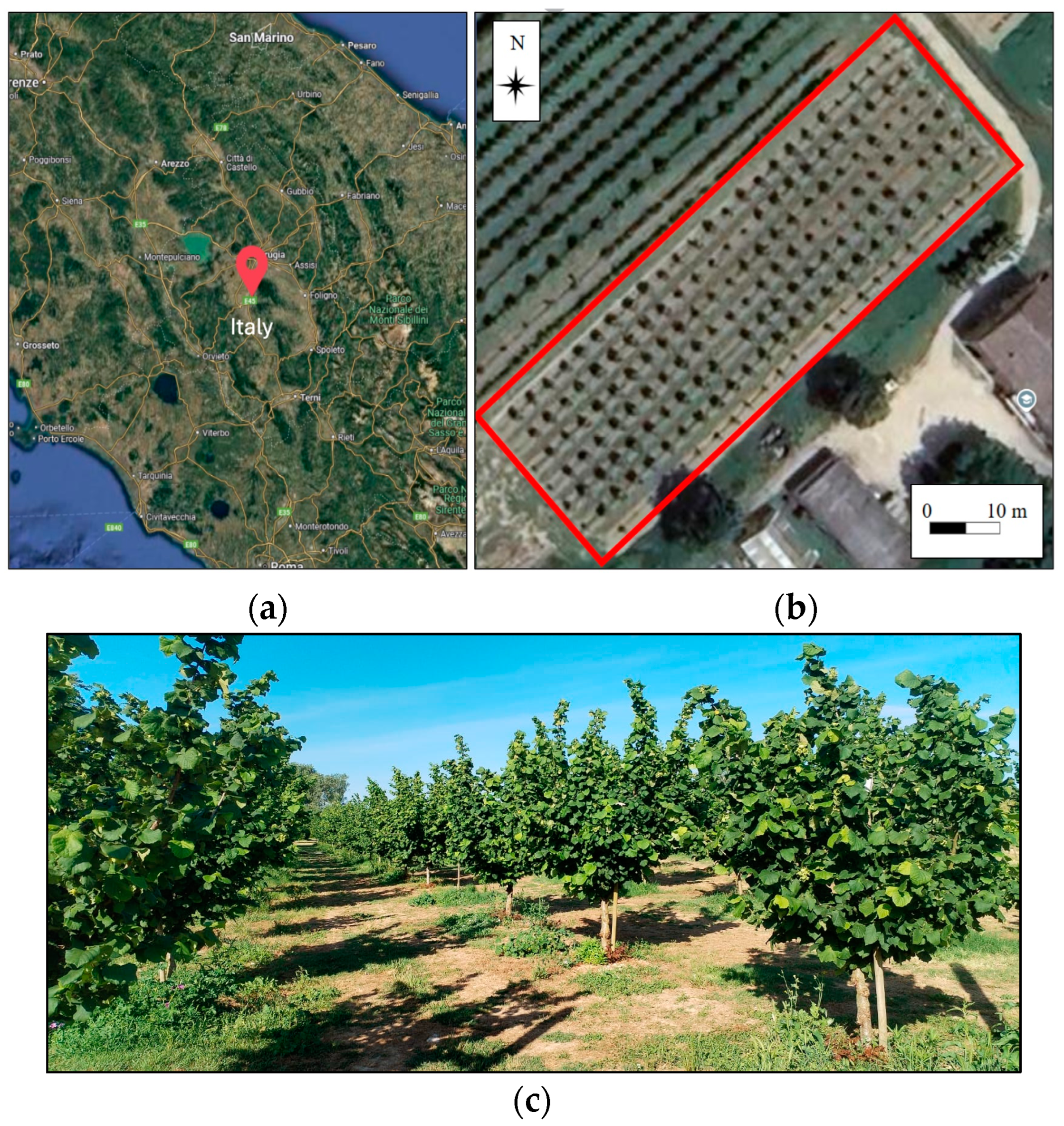
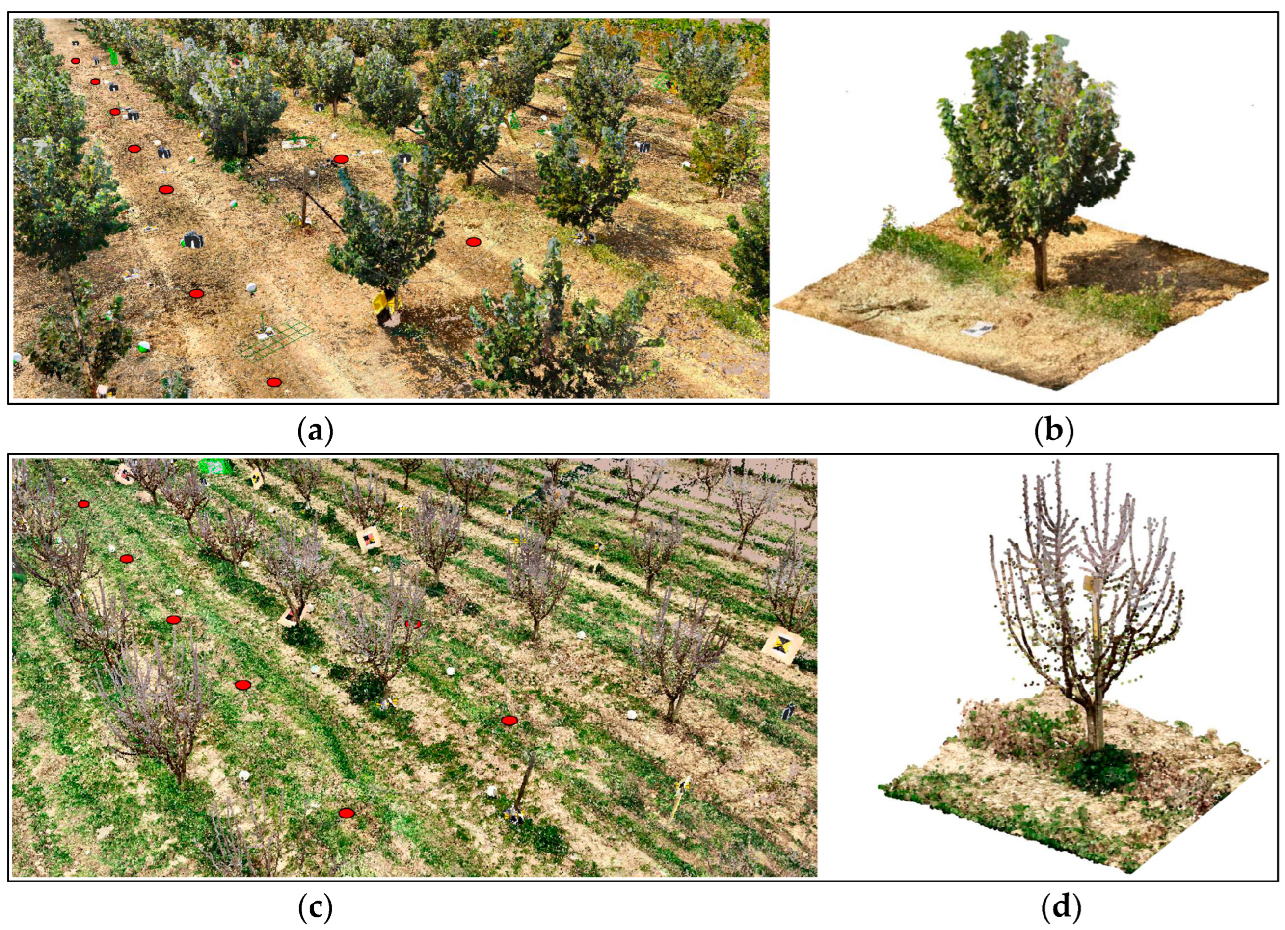
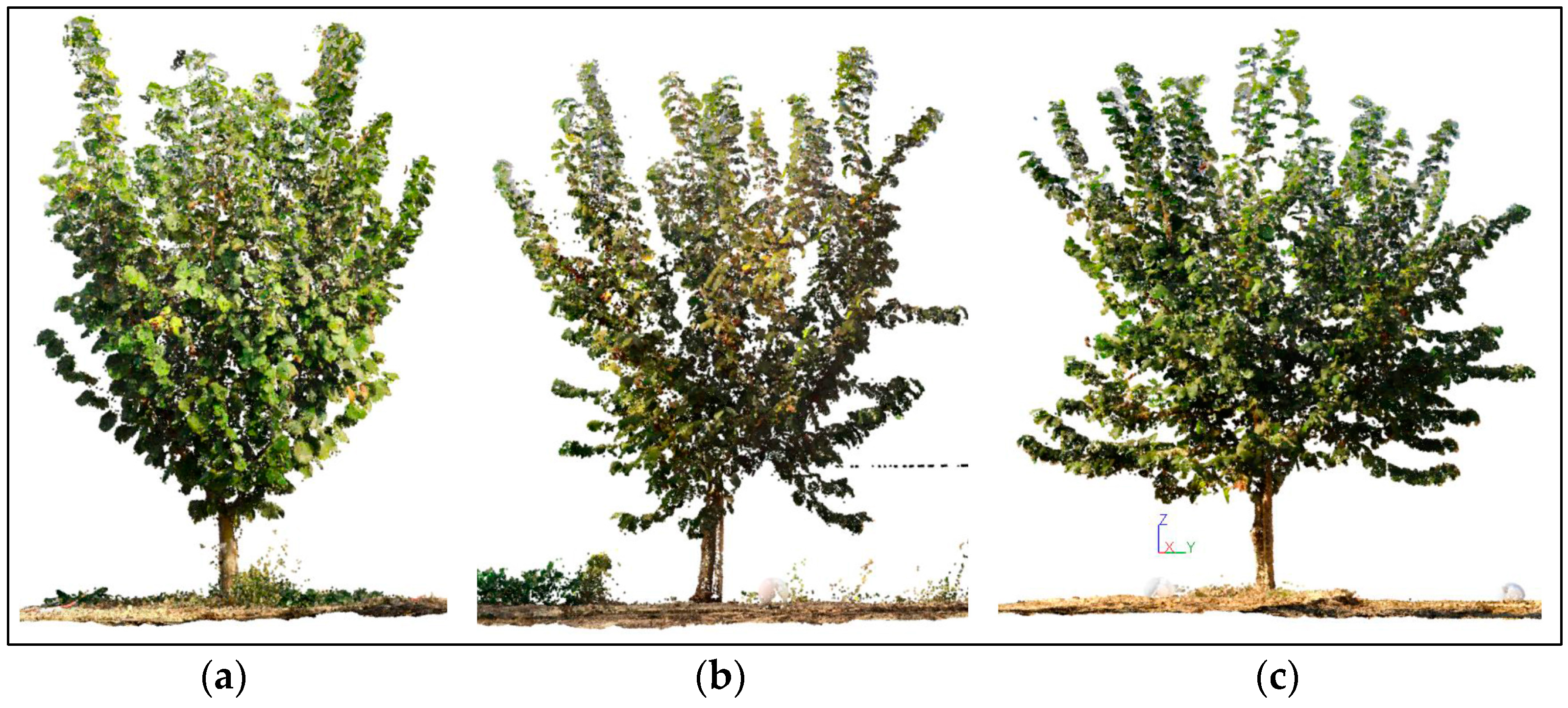
2.1. Study Area and Data Acquisition

This study was carried out in an experimental hazelnut orchard located in Deruta (PG), in central Italy (latitude 42°58′20.0″ N, longitude 12°24′11.1″ E—WGS84) at 163 m a.s.l. (Figure 2), managed by the University of Perugia and supported by Vivai Piante Battistini Società Agricola S.S (Cesena, Italy). The orchard was established in February 2020 with a planting density of 714 trees ha⁻¹, spaced 4 m between rows and 3.5 m on the row, and trained with a single trunk. At the time of the survey, the plants had already completed their structural development, i.e., primary and secondary branches were fully developed [39].

The trees were planted applying a split plot experimental design, where the main treatment was represented by three types of plant material (with a main block of 12 plants per type of plant material), as described later. The second treatment was represented by four hazelnut cultivars. As reported later, within each block defined by plant typology, there were three plants for each cultivar. The orchard was irrigated and managed according to good agricultural practices. Fertilization was applied, considering that the soil is sandy–silty, with a good amount of potassium and an average amount of phosphorus according to the recommendation for the crop [40]. The soil was kept grassed between the rows and hoed under the rows. The climatic characteristics of the area were reported by [40] and are a very hot summer and cold winter, while rainfall is spread in fall and springtime.

According to another study [18], which used 3 trees per cultivar/plant-type combination, and considering that the first aim was, first of all, to set up a methodology using laser scanning, thirty-six hazelnut trees were selected among the following cultivars: Tonda Gentile delle Langhe (hereafter referred to as TGL or T.G. Langhe), Tonda di Giffoni (hereafter referred to as TG or T. Giffoni or Tonda Giffoni), Tonda Francescana^® (hereafter referred to as TF or T. Francescana) and Tonda Gentile Romana (hereafter referred to as TR or T. Romana). All these plants are of the same age and have been managed using the same agronomic techniques and grown in the same environmental conditions. TGL and TG, according to the descriptors for hazelnut [37], are classified as having an intermediate tree vigour and branching density, while TR has a low tree vigour and sparse branching density. TF^® is a new cultivar obtained by crossing TG × TR, so its growth habit has not been defined yet.

Each cultivar was composed of three types of plant material obtained through in vitro propagation (hereafter referred to as micropropagated plant—M) by English double-cleft winter grafting on Corylus colurna L. rootstock (hereafter referred to as grafted plant—G) and by stump layering obtaining n rooted suckers (hereafter referred to as own-rooted plant—O) [40]. Micropropagated plants and rooted suckers are both own-rooted plants having a bushy form, but they show different rates of uniformity, according to [40], with a superficial and fasciculate root system and the ability to produce new suckers from the bottom part of the tree every year [41]. On the contrary, the grafted plants are characterized by the lack of sucker production, a single trunk shape and a deep root system [41].

In total, 9 plants per cultivar were studied, and 12 grafted plants per type of plant, 12 micropropagated plants and 12 own-rooted plants were evaluated. The studied plants were chosen randomly within each block.

The most important differences known about growth descriptors [37] among these three types of plant are that, according to a recent study [40], the grafted plants, regardless of the cultivars, showed an erect growth habit, whereas the own-rooted and micropropagated ones exhibited a semi-erect canopy; no data are available about branch density.

Two laser scanning surveys were conducted, one in October 2023, when the plants had leaves, and the other in March 2024, when budbreak had not yet begun and, therefore, the leaves were not yet present on the trees, following winter pruning. The first survey captured the geometric features of the canopy (height, surface and volume), while the second focused on the trunks and branches (angle, length and diameter).

The TLS Faro Focus 3D (Faro, Lake Mary, FL, USA) was used, performing four laser scans positioned at the four edges of each tree. The scan resolution was set to approximately 7 mm at 10 m (

Table 1. Specifications of the FARO Focus3D X130 laser scanner.

Laser Scanner	Range (m)	Measurement Speed (pts/s)	Ranging Error 1 (mm)	Ranging Noise 2 (mm)	Beam Divergence (mrad)	Point Distance 3 (mm/10 m)
Faro Focus 3D X130	up to 130	up to 976,000	±2	0.3–0.5	0.19	7.00

¹ Defined as a systematic measurement error at around 10 m and 25 m, one sigma. ² Defined as a standard deviation of values from the best-fit plane, based on a measurement speed of 122,000 points/s. ³ Defined as the scan resolution set for the surveys conducted.

). Checkerboard targets and spheres (Figure 3a,b) were employed to align the individual scans into a single, unified point cloud.

The same trees were also measured using manual tools such as a measuring pole with a metric scale marked in cm. Specifically, the average canopy diameter, trunk diameter and height, total tree height and canopy height (calculated as the difference between tree height and trunk height) were recorded to perform a comparison with the geometric features extracted from the laser scanning survey.

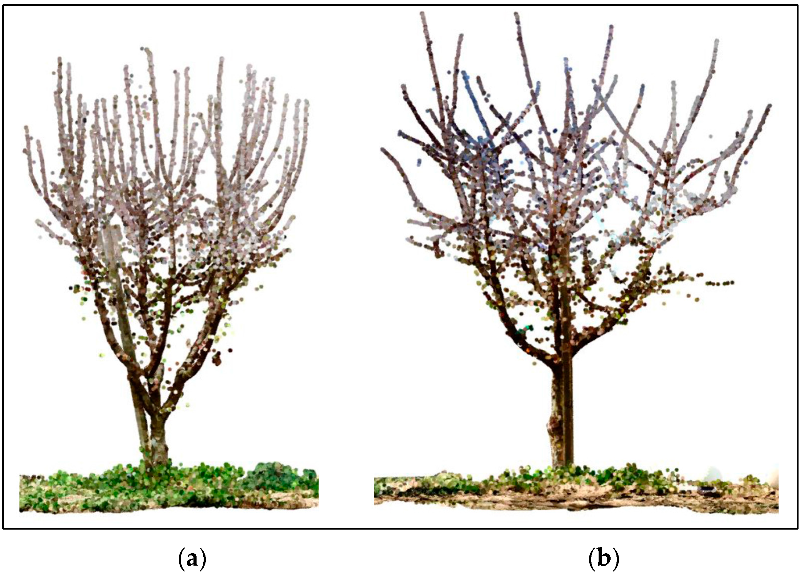
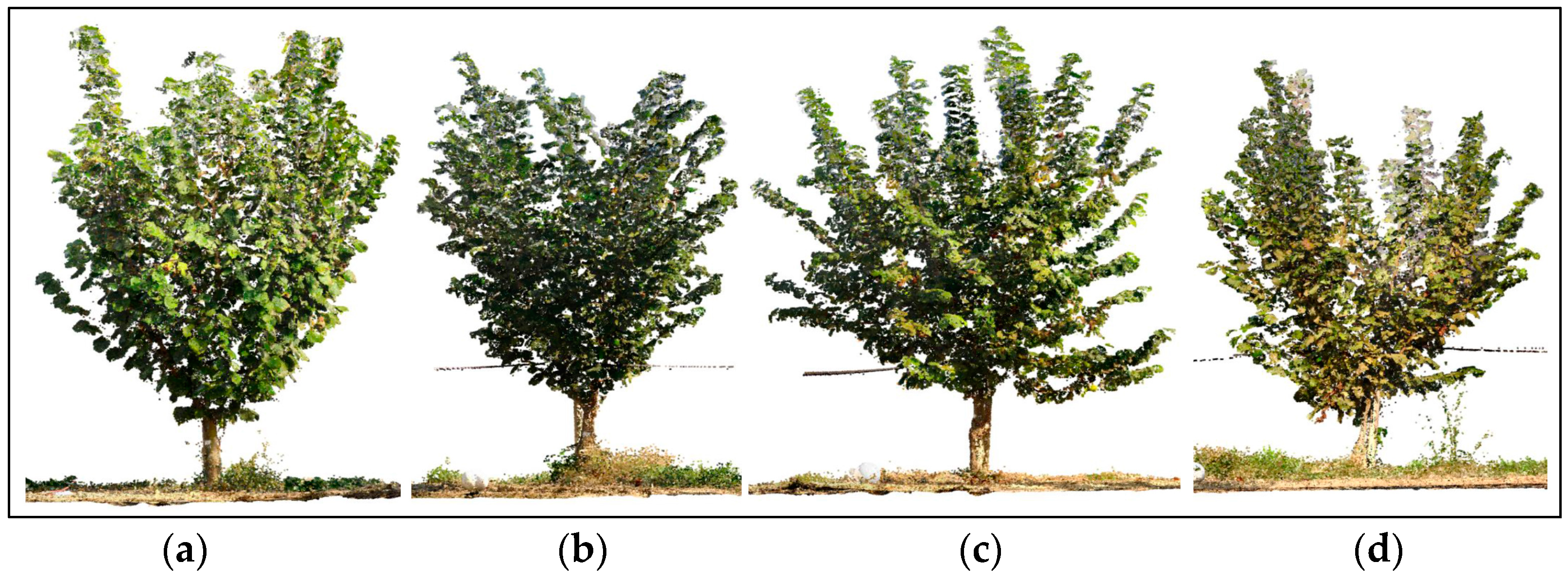
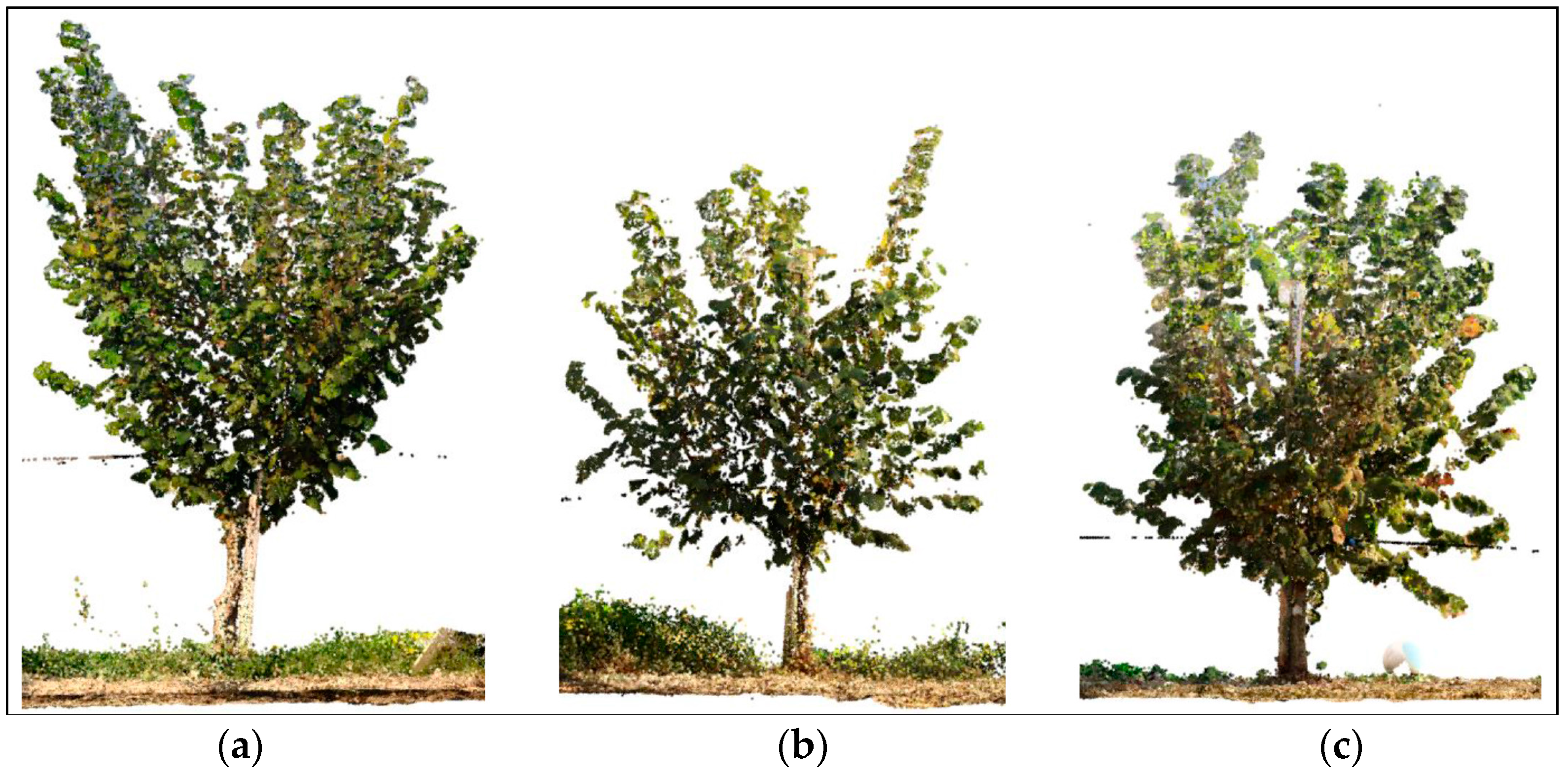
2.2. Point Cloud Generation and Geometrical Feature Extraction

The laser scans were processed using Faro Scene software v. 2021.4.0 (Faro), which automatically recognizes spheres and checkerboard targets for alignment (Figure 4a,c) in a local coordinate system. The resulting average planimetric and altimetric errors were approximately 1.62 cm and 0.61 cm for the October 2023 survey, and 1.23 cm and 0.89 cm for the March 2024 survey. The total point cloud was then processed using Cyclone 3DR software v. 1.7.5 (Leica Geosystem—Part of Hexagon), resulting in a mean point spacing of less than 0.5 cm. Subsequently, the point cloud from each survey was segmented to isolate individual trees (Figure 4b,d).

Specifically, for the October 2023 survey, the following geometrical features were extracted for each tree separately (Figure 5 and Figure 6 and

Table 2. Morphological traits.

Code	Traits	Measurement Method
CH	Canopy height (m)	Automatic from canopy point cloud
CA	Canopy area (m2)	Automatic from canopy point cloud projection
CV	Canopy volume (m3)	Automatic from canopy point cloud
bmin	Minimum planimetric dimension of the canopy projection (m)	Automatic from canopy point cloud projection
bmax	Maximum planimetric dimension of the canopy projection (m)	Automatic from canopy point cloud projection
CW	Canopy width (m)	Automatic from spreadsheet
TS	Trunk section (m2)	Automatic from a horizontal section of the trunk point cloud
BN	Branch number	Manual from tree point cloud
BL	Branch length (m)	Manual from branch point cloud
BLm	Branch length (mean per tree) (m)	Automatic from spreadsheet
BLt	Branch total length (per tree) (m)	Automatic from spreadsheet
α1	Attachment angle of the branches (measured with respect to the vertical direction)	Manual from branch point cloud
α2	Elevation angle of the branches (measured with respect to the vertical direction)	Manual from branch point cloud
BBD	Branch basic diameter (cm)	Manual from branch point cloud
BBS	Basal branch section (cm2)	Automatic from spreadsheet
BVC	Branch volume (cone) (cm3)	Automatic from spreadsheet
LSB	Lateral urface of branches (cm2)	Automatic from spreadsheet
DBm	Mean distance between principal branches (m)	Manual from branch point cloud

):

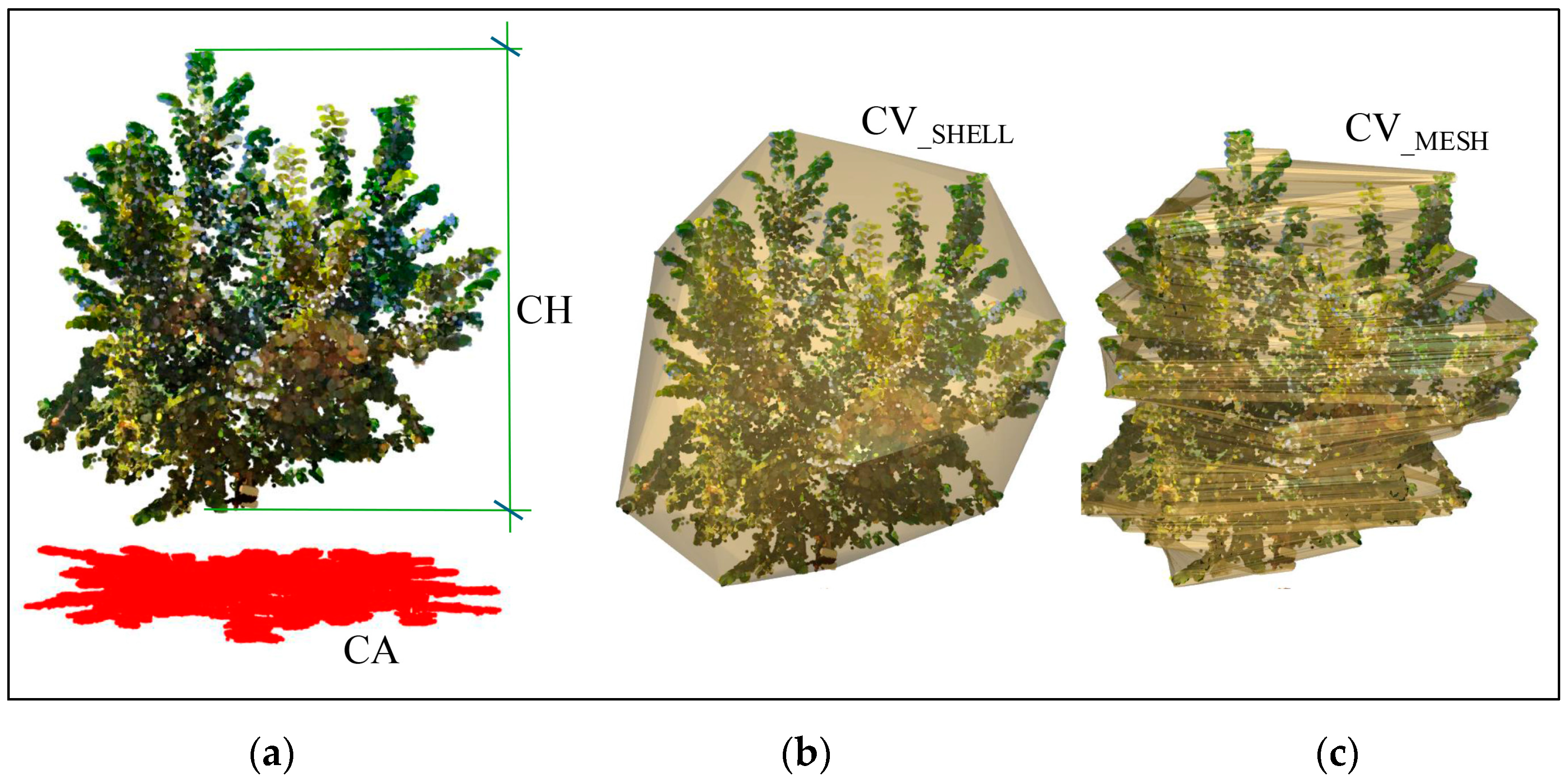
• Canopy height (CH), calculated as the difference between the maximum and the minimum elevation values of the point cloud (Figure 5a);
• Canopy area (CA), determined by measuring the area of the projected canopy point cloud onto a horizontal plane (Figure 5a);
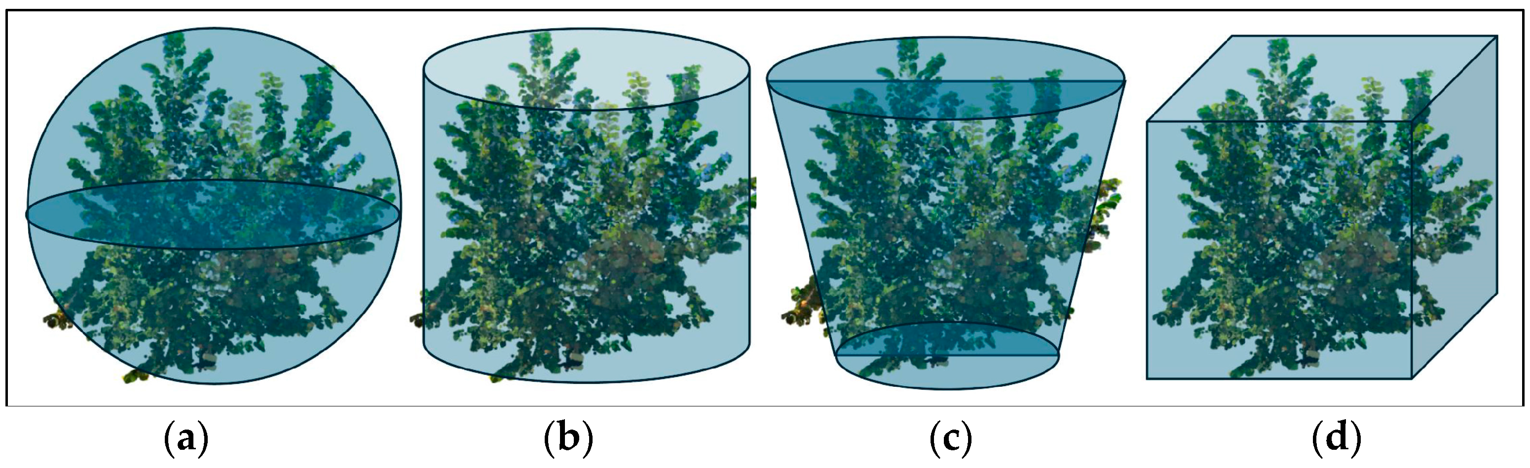
• Canopy volume (CV), estimated using two different approaches: a shell (CV_SHELL), a convex surface enclosing all the canopy points and accounting for the empty spaces between branches (Figure 5b) and a mesh (CV_MESH) derived from the “tree meshing script” in Cyclone 3DR (Figure 5c), which uses horizontal slices with assigned depth at regular intervals in the Z direction;
• bmin and bmax, the minimum and maximum planimetric dimensions, respectively, of a bounding box (the yellow box in Figure 6a,b) around the canopy projection, obtained in a GIS environment;
• Canopy width (CW), the average dimension of the bounding box around the canopy.

The point cloud obtained from the March 2024 survey was used to extract the following features (Figure 7 and Table 2):

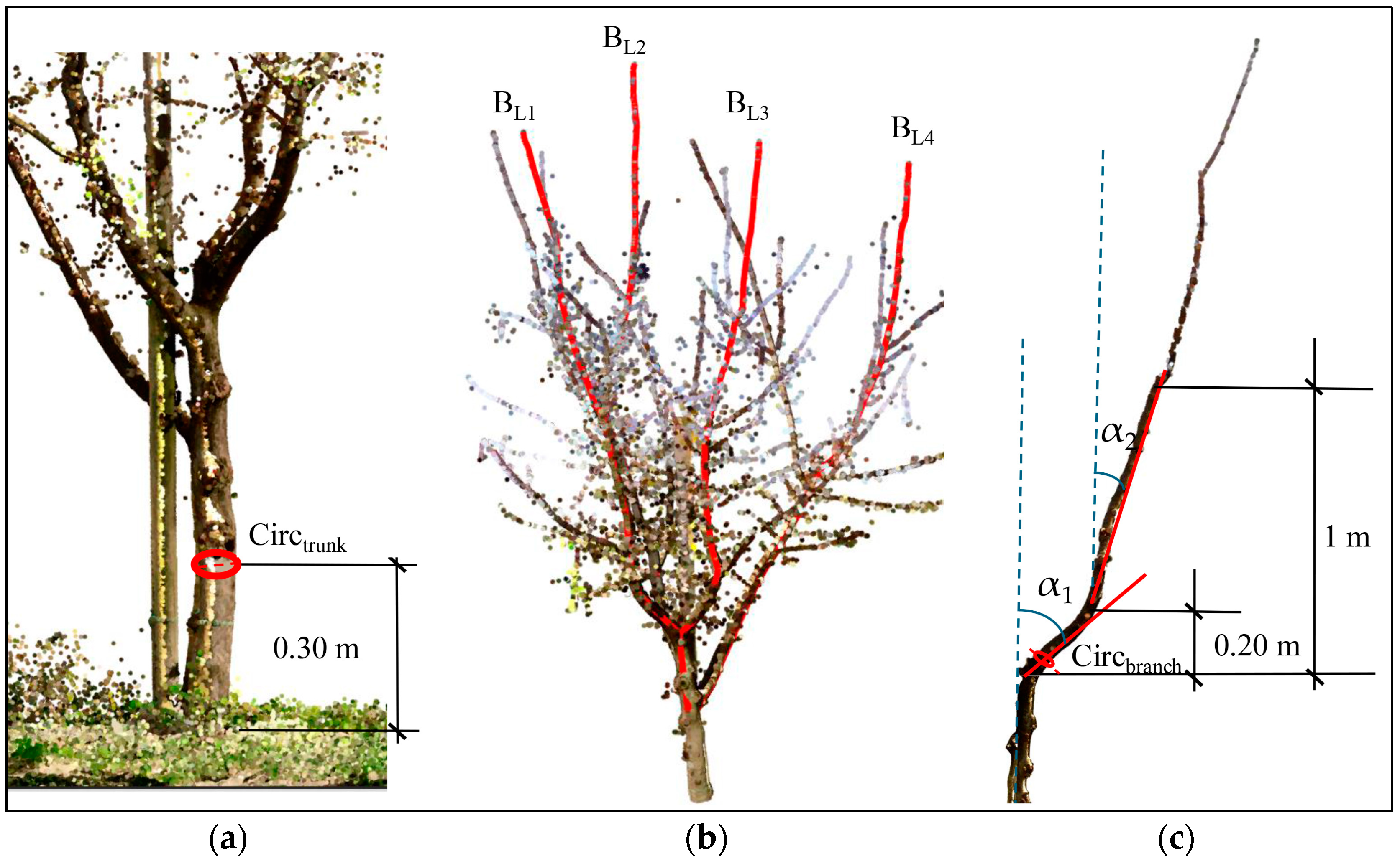
• Trunk circumference at 30 cm from the ground and the relative trunk section (TS) (Figure 7a);
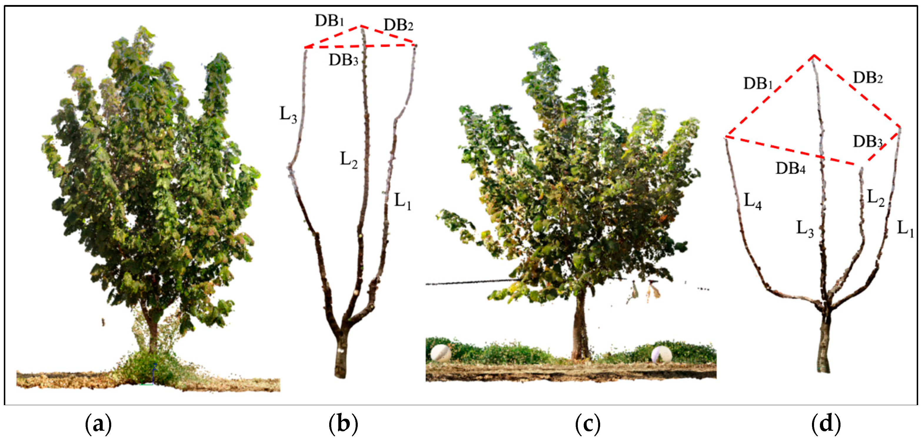
• The number of the principal branches (BN) and the respective length (BL) (Figure 7b), where principal branches are defined as those that are inserted directly on the trunk and constituting the permanent constituent portion of the plant;
• The mean value of the branch length (BLm) and the total length of the branches (BLt) for each tree;
• The branch angles, including the attachment angle (α1, calculated over an ~20 cm segment from the trunk attachment) and the elevation angle (α2, calculated over an ~1 m segment from the trunk attachment), both measured with respect to the vertical direction (Figure 7c);
• The circumference of the principal branches (Figure 7c) and the corresponding branch basic diameter (BBD) and basal branch section (BBS);
• The branch volume (BVC) and the lateral surface (LSB) of each principal branch, considered as a cone with a base area equal to BBS and a height equal to BL;
• The mean distance between principal branches (DBm) (Figure 8).

In Table 2 “Automatic” refers to operations performed using dedicated software tools or scripts with minimal user interaction (e.g., selecting the relevant point cloud and executing a predefined tool). “Manual” indicates traits measured directly by the operator on the 3D point cloud, involving user-driven identification or delineation of specific structures.

Morphological traits CH, CA, CV, bmin, bmax, CW, TS, BN, BL, BLm, BLt, BBD, BBS, BVC and LSB provide information regarding tree vigour; α1, α2 and DBm can help to define tree growth habit; while BN and BL can be used to evaluate branch density. Specifically, α1 was used to discriminate the plant growth habit, expressed as the percentage of branches falling in each class relative to the total. Growth habit was classified as erect when α1 was <35°, semi-erect between 35° and 55°, spreading between 55° and 75° and drooping when α1 was >75°.

This classification was developed following the guidelines suggested for other fruit tree species, such as peach, using the descriptors indicated in the Bioversity descriptor manual considering, however, the different habitus of the fruit tree species [18,37,42].

The calculation of previously defined morphological indices (Table 2) was based on a combination of automated and manual operations. The separation between canopy and trunk was performed manually. Features such as ground extraction, individual tree segmentation, canopy projection, bounding box, canopy height and volume, trunk circumference and branch volume were computed automatically using point cloud processing software (Cyclone 3DR, QGIS v. 3.34.15 and spreadsheet tools).

In particular, point cloud refer to the ground and terrain mesh were extracted using the DTM tool in Cyclone 3DR, which generates a digital terrain model by creating a mesh from the lowest Z values in the point cloud. Tree segmentation was then carried out in two automated steps: first, the terrain mesh was duplicated and vertically shifted to isolate the above-ground points representing vegetation; second, the ‘Distance’ tool was used to separate the point cloud into individual trees based on point proximity [33].

Canopy area was derived by projecting the canopy points onto the horizontal plane and extracting the crown contours in Cyclone 3DR, while area measurement was performed in QGIS. Canopy volume was automatically calculated using the “Tree Meshing” script and the “Convex Hull” tool in Cyclone 3DR. Canopy height was directly obtained from the point cloud attributes [33].

In contrast, the following traits required manual identification and measurement directly on the 3D point cloud: the separation of main branches, the measurement of their angles and lengths and the determination of the bounding branch diameter.

2.3. Morphological Indexes

From the geometric features of the trees extracted from the two surveys, several morphological indexes were calculated (

Table 3. Morphological indexes.

Code	Index	Equation
CS	Canopy symmetry	bmin/bmax
CU	Canopy uprightness	CW/CH
C_HW	Ratio between the height and width of the canopy	CH/CW
C_AV	Ratio between the area and volume of the canopy (m−1)	CA/CV
VPI—E	Volumetric Projection Index—Ellipsoid	CV/Vellipsoid
VPI—C	Volumetric Projection Index—Cylinder	CV/Vcylinder
VPI—CT	Volumetric Projection Index—Cone Trunk	CV/Vcone_trunk
VPI—P	Volumetric Projection Index—Parallelepiped	CV/Vparallelepiped
ICO	Index of Canopy Opening	DBm/BLm
BL_CV	Ratio between the total branch length and the canopy volume (m−2)	BLt/CV
LSB_CV	Ratio between the lateral surface of all the branches and the canopy volume (cm−1)	LSB/CV
BBS_CV	Ratio between the basal section of the branches and the canopy volume (cm2/m3)	BBS/CV
BBS_TS	Ratio between the basal section of the branches and the trunk section	BBS/TS
BN_CA	Ratio between the number of branches and the canopy area (m−2)	BN/CA
BN_CV	Ratio between the number of branches and the canopy volume (m−3)	BN/CV
BVC_CV	Ratio between branch volume and canopy volume (cm3/m3)	BVC/CV

). Some of these indexes have been previously proposed or described in different forms in the literature [28,43,44,45], while others were developed and proposed in this study for use with hazelnut. Here, some of the morphological indexes used are renamed using new acronyms to align with the specific aims of this study. Specifically, the following indexes were developed and proposed for hazelnut:

• CS (Canopy Symmetry), defined as the ratio between the minimum and the maximum planimetric dimension of the canopy projection;
• CU (Canopy Uprightness), defined as the ratio between the canopy width (CW) and the canopy height (CH);
• C_HW, defined as the ratio between the height (CH) and width of the canopy (CW);
• C_AV, defined as the ratio between the area (CA) and volume of the canopy (CV);
• VPI (Volumetric Projection Index), calculated as the ratio between the canopy volume and the volume of four “ideal” geometric shapes: ellipsoid (VPI-E), cylinder (VPI-C), cone trunk (VPI-CT) and parallelepiped (VPI-P), as shown in Figure 9a, Figure 9b, Figure 9c and Figure 9d, respectively;
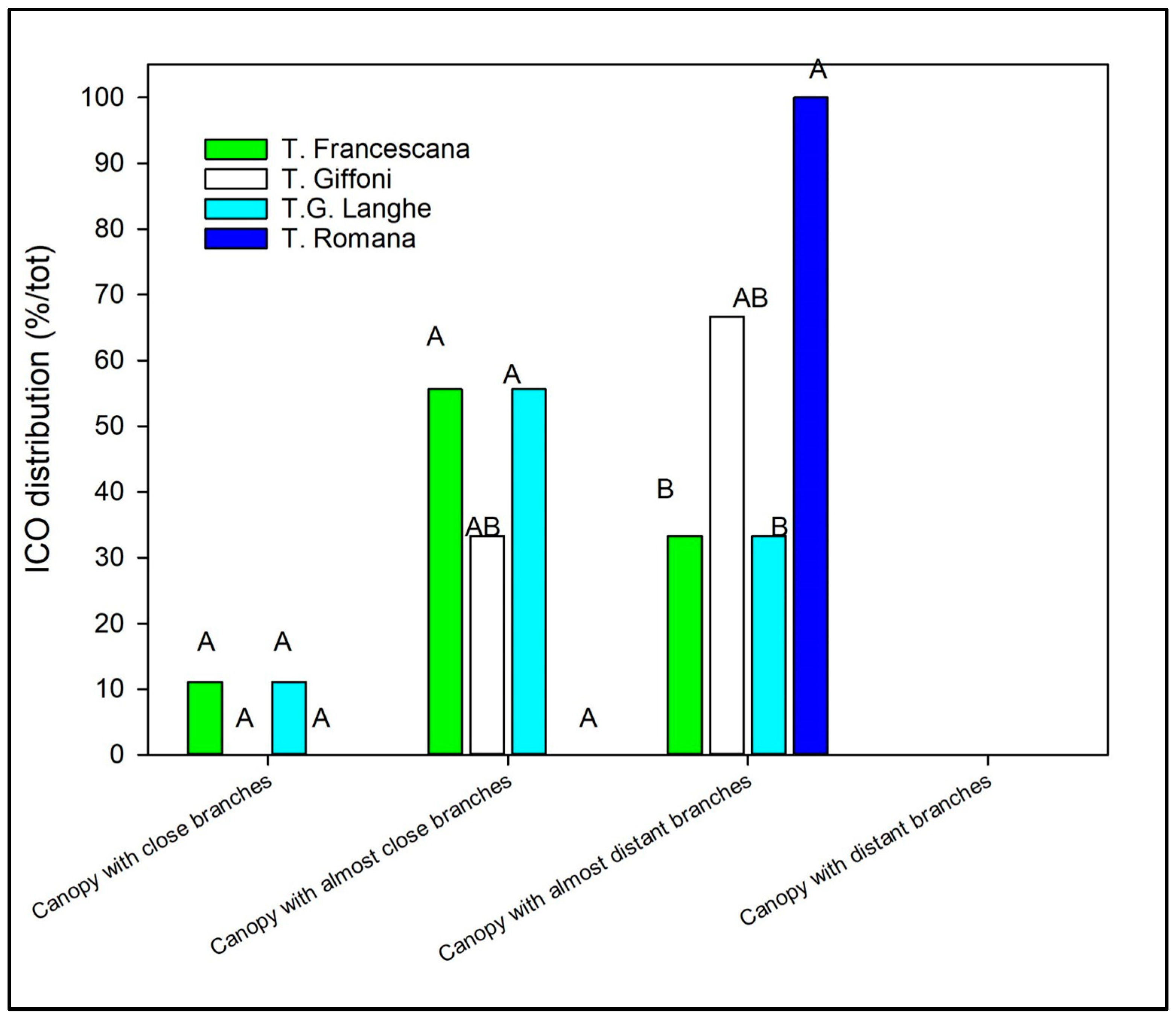
• ICO (Index of Canopy Opening), calculated as the ratio between the average distance between adjacent branches (DBm) and the average branch length (BLm);
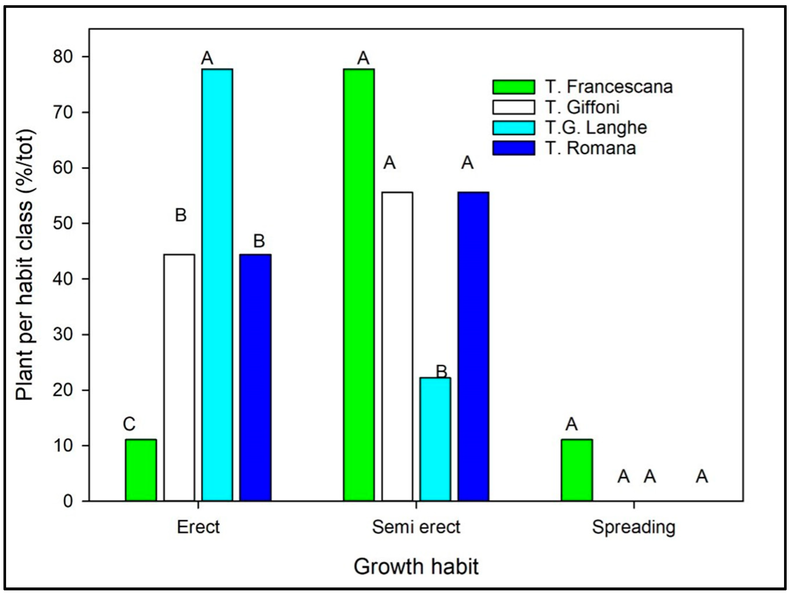
• ICO was used to define the canopy habit, expressed as the number of branches falling in each class relative to the total. If ICO was <0.35, the canopy was classified as “canopy with close branches”; ICO between 0.35 and 0.45 indicated a “canopy with almost close branches”; ICO between 0.45 and 0.55 indicated “canopy with almost distant branches”; and ICO > 0.55 indicated a “canopy with distant branches”;
• BL_CV, calculated as the ratio between the total length of branches (BLt) and the canopy volume (CV);
• LSB_CV, calculated as the ratio between the lateral surface of all the branches (LSB) and the canopy volume (CV);
• BBS_CV, calculated as the ratio between the basal branches section (BBS) and the canopy volume (CV);
• BBS_TS, calculated as the ratio between the basal section of the branches (BBS-TS) and the trunk section (TS);
• BN_CA, calculated as the ratio between the number of branches (BN) and the canopy area (CA);
• BN_CV, calculated as the ratio between the number of branches (BN) and the canopy volume (CV);
• BVC_CV, calculated as the ratio between branch volume (BVC) and canopy volume (CV).

Regarding these parameters, the following can be stated:

• CS values close to 1 indicate symmetry, while lower values reflect asymmetry in the canopy projection onto a horizontal plane;
• Higher CU values indicate a less compact canopy, while lower values reflect a more compact structure;
• Higher C_HW values indicate a more slender canopy, while values close to 1 indicate constant proportions between height and width;
• Larger C-AV values correspond to a less compact canopy, whereas smaller values indicate a denser structure;
• VPI values close to 1 indicate that the ideal solid closely approximates the canopy shape;
• Lower ICO values correspond to a more compact canopy with close branches;
• The values of BL_CV, LSB_CV, BBS_CV, BBS_TS, BN_CA, BN_CV, and BVC_CV provide information regarding branch density.

2.4. Statistical Analysis and Principal Component Analysis

The proposed morphological traits and morphological indexes (Table 2 and Table 3) were applied to 36 plants, and the obtained data were statistically analysed using ANOVA and considering two factors, namely cultivar and plant type. Means were compared using the Duncan test. Statistical analysis was performed per type of plant material and per cultivar to evaluate whether the suggested indexes could discriminate among the hazelnut plant traits, both among cultivars and among plant types, as well as to assess the validity of the proposed methodology of trait classification.

Principal component analysis (PCA) was performed using morphological traits as input variables to explore the variability among samples and to detect the most discriminating variables. PCA summarizes the information contained in the data matrix in fewer independent PCs, obtained as linear combinations of the original variables, oriented in the direction of maximum variance [46]. The data were statistically evaluated using R v.3.5.1 (R Core Team, 2018).

3. Results and Discussion

3.1. Definition of the Hazelnut Plant Traits by the Application of Morphological Traits and Morphological Indexes

The morphological traits and morphological indexes that were measured and calculated per each plant and cultivar (listed in Table 2 and Table 3), were useful in defining plant traits but not always capable of discriminating cultivars or plant types.

In particular, branch number (BN) was similar among the four cultivars, even if it was 3.3 in TR and around 3.7 in the other three cultivars (

Table 4. Branch number (BN), branch basic diameter (BBD), attachment angle of the branches (α1), elevation angle of the branches (α2), ratio between canopy height and canopy width (C_HW), Index of Canopy Opening (ICO), canopy symmetry (CS), canopy uprightness (CU), and ratio between canopy area and canopy volume (C_AV).

Cultivar/ Plant Type	BN (n)	BBD (cm)	α1 (°)	α2 (°)	C_HW	ICO	CS	CU	C_AV
TF	3.7 A	3.65 A	46.4 A	24.8 A	1.32 A	0.446 BC	0.94 A	0.90 A	0.52 C
TG	3.7 A	3.16 B	39.0 B	21.7 AB	1.28 A	0.514 AB	0.94 A	0.89 A	0.64 A
TGL	3.8 A	3.63 A	39.1 B	19.8 B	1.36 A	0.433 C	0.96 A	0.81 B	0.60 B
TR	3.3 A	3.13 B	41.2 AB	23.1 AB	1.34 A	0.529 A	0.91 A	0.86 AB	0.66 A
G	3.7 a	3.54 a	38.0 b	23.1 a	1.29 a	0.494 a	0.95 a	0.87 a	0.60 a
M	3.5 a	3.42 ab	41.0 ab	21.4 a	1.34 a	0.444 a	0.93 a	0.86 a	0.61 a
O	3.7 a	3.21 b	45.2 a	22.5 a	1.34 a	0.504 a	0.94 a	0.87 a	0.61 a

In each column, different lowercase letters indicate significant (p < 0.05) differences among types of plant. Different uppercase letters indicate significant (p < 0.05) differences among cultivars.

). Since the differences in branch number were found not to be statistically dependent on the cultivar, as highlighted by identical capital letters in Table 4, this trait resulted was not useful for defining canopy shape and branching in trained plants. Similarly, the number of branches per plant was not different among the three types of plants (Table 4), as indicated by identical lowercase letters next to the mean values in the table.

The branch basic diameter (BBD), however, allowed us to distinguish two groups of cultivars: one composed of TF and TGL, with an average of 3.64 cm, and one composed of TG and TR, with an average of 3.14 cm (Table 4). The BBD was different between grafted and own-rooted plants, while the micropropagated plant showed a similar BBD. However, in fact, they are both own-rooted plants produced through two different propagation techniques (layering and in vitro propagation). This behaviour could depend on the characteristics of own-rooted plants; in fact, these are also called rooted sucker plants, which are very different from each other. In contrast, the in vitro propagation by tissue culture or micropropagation as a method of vegetative propagation of plant or fruit species allows for the production of uniform clones [40,47].

The BBD trait could be also used to determine tree age, as suggested for forest trees, based on increments in branch size, and it can be measured on both young and old hazelnut plants [48].

The attachment angle of the branches (α1) allowed us to distinguish two groups of cultivars: one with a narrow angle α1, around 39°, composed of TGL and TG cultivars, and one with a wider angle α1, from 41.2° to 46.4°, composed of TF and TR cultivars (Table 4 and Figure 6). Moreover, the grafted plants showed a narrower angle with respect to that measured on own-rooted ones according to observations on hazelnut reported by [41]. On the contrary, no clear influence of rootstock on branch angle was observed in almonds [18].

According to the descriptor of tree growth habit, illustrated in paragraph 6.1.2 of Descriptors for Hazelnut [37], this trait includes six types of growth habit (very erect, erect, semi-erect, spreading, drooping and contorted), and they are defined using a reference cultivar for each type of habit (Figure 10). TGL, TG and TR are classified as having a semi-erect growth habit. In contrast, the measurement of α1 shows that TGL and TG have a narrower average attachment angle of the branches than that measured in TR plants (Table 3 and Figure 6).

Regarding the α₁ angle, a range was hypothesized for each growth habit class: erect when the angle between trunk and branches (α₁) is <35°; semi-erect between 35° and 55°; spreading between 55° and 75°; and drooping when the angle is >75° (Figure 11). This classification was obtained not on the mean value of α₁, but on the number of branches falling in each class, with respect to the total.

Based on this classification, the TGL showed an erect habitus, with 77.8% of α₁ values < 35° and TF exhibiting a semi-erect habitus, with 77.8% of α₁ values between 35° and 55° (Figure 12). The growth habit of the other two cultivars was between erect and semi-erect.

With respect to the tree growth habits reported in the Descriptors for Hazelnut [37], the use of α₁ allows for better discrimination of the habitus of the different cultivars; in fact, the TGL, TG and TR cultivars are reported as having the same habitus, namely semi-erect, while TGL clearly shows an upright habit (Table 4 and Figure 12).

The elevation angle of the branches, α₂, allowed discrimination between TF and TGL cultivars (Figure 13); in fact, TF showed an α₂ of 24.8°, while TGL showed 19.8° (Figure 7 and Table 4), confirming the growth habit of the TGL cultivar as erect, since α₂ also proved to be narrow, similar to α₁, and the growth habit of the TF cultivar is semi-erect.

It must be considered that the branch angle is a complex trait regulated by several processes, where light perception and gravity sensing play a major role and are primarily regulated in the aerial parts of the plant [18].

The ratio between canopy height and canopy width (C_HW) indicates the canopy slenderness in forest trees, where growth is more pronounced in height than in width [49] (Table 4). This ratio may also indicate the consistency of the canopy shape, meaning whether the canopy maintains constant proportions between height and width in different plants. In olive trees, this ratio defines the canopy shape index: if C_HW > 1, canopy shape is attributed to a cylinder with an elliptical basis; while if C_HW < 1, the canopy shape is attributed to an ellipsoidal shape [9]. According to this classification, all the cultivars studied show a canopy shape resembling a cylinder with an elliptical basis, the ratio always being >1 (Table 4). Moreover, no differences were observed among the cultivars and even among the plant types for the C_HW ratio. This could be due to the lack of restriction by, for example, factors such as water, light or nutrients, since the plants were still young (only 5 years old) and well managed [43]; therefore, this trait seems to be unsuitable for describing the structure of hazelnut plants.

The Index of Canopy Opening (ICO) (Figure 10) ranged from 0.43 to 0.53 and significantly varied among the four cultivars, while it was similar among the three plant materials (Table 4). The canopy habit, on average, resulted in a canopy with almost distant branches on TR and TG cultivars, with almost close branches on TGL and TF cultivars.

3.2. Assessment of Geometric Models of Canopy Volume That Best Reproduce TLS Estimates

Regarding the two different models used for volume estimation from TLS point clouds, when comparing the values obtained from CV_SHELL with those estimated using CV_MESH, it was observed that, on average, the former were approximately 10% higher than the latter. Furthermore, the differences between the canopy volumes obtained through manual measurements (which assume a cylindrical canopy shape) and those derived from the laser point clouds (CV_SHELL and CV_MESH) were evaluated.

Comparing the mean and standard deviation of the differences in canopy volume, the values obtained using CV_SHELL (0.786 m and 1.004 m for mean and standard deviation, respectively) show a greater deviation from those obtained through manual measurements, with higher statistical values compared to the differences derived from CV_MESH (0.374 m and 0.798 m for mean and standard deviation, respectively) (Figure 13). For this reason, the tree meshing script was chosen for the subsequent analysis of the canopy shape.

The C_AV ranged from 0.52 to 0.66, and the TG and TR cultivars showed plants with less compact canopy, having the highest index values, while TGL and TF exhibited a denser canopy structure (Table 4).

The Volumetric Projection Indexes (VPIs) were used to establish which geometric shape best described the canopy of the hazelnut tree. Specifically, the best assumption is that the hazelnut canopy shape could resemble an ellipsoid (VPI-E), a cylinder (VPI-C), a cone trunk (VPI-CT) or a parallelepiped (VPI-P) (

Table 5. Canopy shape according to the Volumetric Projection Index per cultivar and plant type.

Cultivar/ Plant Type	VPI—E	VPI—C	VPI—P	VPI—CT
TF	1.18 A	1.77 A	2.25 A	1.11 A
TG	1.10 A	1.65 A	2.09 A	0.91 B
TGL	1.11 A	1.67 A	2.13 A	0.94 B
TR	1.14 A	1.72 A	2.17 A	1.07 A
G	1.11 a	1.66 a	2.11 a	0.93 b
M	1.13 a	1.70 a	2.16 a	1.05 a
O	1.16 a	1.75 a	2.22 a	1.03 a

In each column, in plant type and cultivar, means followed by different letters are significantly different at p < 0.05. Different uppercase letters indicate significant (p < 0.05) differences among cultivars. Different lowercase letters indicate significant (p < 0.05) differences among types of plant.

).

The modelled parallelepiped canopy volume (VPI-P) and the modelled cylinder canopy volume (VPI-C) overestimated the geometric model since their values were very far from the value of 1; this means that the assumption was incorrect (Table 5). These results agree with those obtained by Owen and Lines [44] in mixed Mediterranean forests, where cylinders produced large overestimations for both concave and convex canopies.

Among all the ideal solids considered, the ellipsoid (VPI-E) and the cone trunk (VPI-CT) most closely approximate the shape of the hazelnut canopy, since their VPI values are close to 1. However, VPI-CT is the only one that is capable of discriminating canopy shape among different cultivars and plant types (grafted or own-rooted) (Table 5). Specifically, VPI-CT discriminates the canopy shapes of TF and TR cultivars (on average VPI-CT was 1.09) from those of TGL and TG cultivars (on average VPI-CT was 0.92) (Figure 14).

VPI-CT also distinguishes the canopy of grafted plants (0.93) from that of own-rooted plants (1.04 in average) (Table 5 and Figure 15).

VPI-CT was very useful in defining the best geometric model for tree canopy, which until now had been established using the ratio C_HW (Table 4). According to the C_HW values, the geometric model for the hazelnut canopy was a cylinder with an elliptical base, showing no difference among the hazelnut cultivars, unlike what has been observed in olive cultivars (Table 4) [9].

Considering the ICO distribution as number of plants per class (%/tot) (Figure 16), the TGL and TF cultivars have 55.6% of plants with almost close branches and 11.1% with close branches. TG has 66.7% of plants with almost distant branches and 33.3% with almost close branches. The TR cultivar has a unique distribution, with all plants falling in the same ICO class, which is characterised by a canopy with almost distant branches (Figure 16). Therefore, it can be said that the canopy habit was well described by the Index of Canopy Opening (ICO).

CS ranged from 0.91 to 0.96 among the cultivars and from 0.93 to 0.95 among the plant types, showing no statistical differences (Table 4). Considering that CS values close to 1 indicate symmetry, the data show that all plants have a symmetrical canopy, and those of the TGL cultivar were the most symmetric. This trait was affected by the presence of restriction such as light, agronomic management practices such as pruning and even age [3,43,50]. Therefore, this trait could be more useful for evaluating the correctness of canopy management within an organized plantation than for breeding evaluation.

Canopy uprightness (CU) ranged from 0.81 to 0.90, and the TGL cultivar showed the lowest value, which as significantly different from those of TF and TG, confirming that the TGL cultivar has a more compact structure compared to those of the other cultivars, since lower values reflect a more compact structure (Table 4). CU was not different in the three types of plants, regardless of the cultivars (Table 4).

The basal branch section (BBS) allowed us to distinguish two groups of cultivars: one group with greater BBS (10.6 cm²), and therefore greater vigour, composed of TF and TGL cultivars; and one with smaller BBS (7.9 cm²), composed of TG and TR cultivars (

Table 6. Basal branch section (BBS), lateral surface of branches (LSB), branch volume cone (BVC), branch length (mean per tree) (BLm), branch total length (per tree) (BLt), ratio (BL_CV) between the total branch length (BLt) and the canopy volume (CV), LSB_CV = ratio between the lateral surface of the branch length (LSB_CV) and the canopy volume (CV).

Cultivar/ Plant Type	BBS (cm2)	LSB (cm2)	BVC (cm3)	BLm (m)	BLt (m)	BL_CV (m/m3)	LSB_CV (cm2/cm3)
TF	10.6 A	1334 A	825 A	2.3 A	7.8 B	1.6 C	0.00096 B
TG	8.0 B	976 B	537 B	1.9 B	8.0 B	2.6 A	0.00112 AB
TGL	10.6 A	1191 A	741 A	2.1 B	9.0 A	2.5 A	0.00123 A
TR	7.9 B	882 B	478 B	1.8 C	5.3 C	2.1 B	0.00111 AB
G	10.1 a	1148 a	700 a	2.1 a	8.3 a	2.1 a	0.0011 a
M	9.4 ab	1107 a	653 a	2.0 a	7.4 b	2.3 a	0.0012 a
O	8.4 b	1031 a	584 a	2.0 a	6.9 b	2.1 a	0.0011 a

In each column, different uppercase letters indicate significant (p < 0.05) differences among cultivars. Different lowercase letters indicate significant (p < 0.05) differences among types of plant.

). Thus, the BBS of the grafted plants was higher (10.1 cm²) than that of the own-rooted plants (8.4 cm²) (Table 6).

Similarly, the lateral surface of branches (LSB) showed a difference between two groups of cultivars: the TF and TG cultivars showed an LSB of around 1263 cm², while TG and TR showed around 929 cm². The same trend was observed for the branch volume cone (BVC) (Table 6). On the contrary, the TF cultivar showed the longest branches, with a mean branch length (BLm) of 2.3 m, while the TR cultivar had the shortest branch, with a mean branch length of 1.8 m. The TG and TGL cultivars’ mean branch lengths were around 2 m (Table 6). Considering, however, the overall branch length per tree (BLt), which is also linked to the number of branches (BN), the TGL cultivar showed the longest value of 9.0 m, followed by TG and TF (Table 6).

The ratio BL_CV between the total length of the branches (BLt) and the canopy volume (CV) may represent an evaluation of the canopy density (Table 6). The highest BL_CV was obtained by the TG and TGL cultivars, around 2.6, followed by the TR cultivar, while the lowest ratio BL_CV was observed in TF (Table 6).

LSB_CV (the ratio between the lateral surface of the branch’s length and the canopy volume) ranged from 0.00096 to 0.00123 (Table 6).

Branching density can be assessed using several traits (

Table 7. Branching density. BN_CA ratio between branches number (BN) and canopy area (CA); BN_CV ratio between branches number (BN) and canopy volume (CV); BBS_TS ratio between basal section of the branches (BBS-TS) and trunk section (TS); BBS_CV ratio between basal section of the branches (BBS) and canopy volume (CV); BVC_CV ratio between branch volume (BVC) and canopy volume (CV).

Cultivar/ Plant Type	BN_CA (n./m2)	BN_CV (n./m3)	BBS_TS	BBS_CV (cm2/m3)	BVC_CV (cm3/m3)
TF	1.4 B	0.7 C	1.1 B	7.6 B	587 B
TG	1.9 A	1.2 AB	1.1 B	9.1 AB	630 AB
TGL	1.7 A	1.0 B	1.6 A	10.9 A	767 A
TR	2.0 A	1.3 A	1.2 AB	10.0 A	595 B
G	1.6 a	0.9 a	1.0 b	9.6 a	659 a
M	1.8 a	1.1 a	1.4 a	10.0 a	670 a
O	1.8 a	1.1 a	1.3 ab	8.7 a	605 a

In each column, different uppercase letters indicate significant (p < 0.05) differences among the cultivars. Different lowercase letters indicate significant (p < 0.05) differences among the types of plant.

). The number of branches per canopy area (BN_CA) ranged from 1.4 to 2.0, and the TF cultivar showed the lowest value, having the largest canopy area (Table 4 and Table 7).

The number of branches per canopy volume (BN_CV) was highest in the TR and TG cultivars (on average 1.2), significantly lowest in the TF cultivar (0.7) (Table 7).

The ratio between the basal branches section (BBS) and the trunk section (TS) varied from to 1.1 to 1.6, and TGL showed the highest value (Table 7). The BBS_TS ratio differed between the grafted and micropropagated plants, consistent with the findings reported by [40].

The ratio between the basal branches section (BBS) and canopy volume (CV) allows us to distinguish the TF cultivar from the TGL and TR cultivars (Table 7).

The ratio between branches volume (BVC) and canopy volume (CV) discriminated the TGL cultivar from the TF and TR cultivars, but did not discriminate grafted plants from the other types (Table 7).

3.3. Plant Traits to Be Used as Standard Descriptors of Hazelnut Cultivar

Based on the results reported above, 19 morphological traits and morphological indexes proved useful in defining, following a scientific procedure, the growth descriptors reported by Bioversity, FAO and CIHEAM (2008) [37] for hazelnut. These are tree vigour, tree growth habit and branching density.

Specifically, among the 18 suggested morphological traits, listed in Table 2, only eight were selected, based on statistical analysis results reported in Section 3.1 and Section 3.2, since they proved suitable to serve as standard hazelnut trait descriptors of tree vigour and tree growth habit, as explained below:

• BBD (branch basic diameter) allowed us to distinguish two groups of cultivars: one group composed of TF and TGL and one composed of TG and TR (Table 4). The BBD was different between a grafted plant and an own-rooted plant.
• BBS (basal branch section) also allowed us to differentiate two groups of cultivars: one group with greater BBS, and therefore greater vigour, composed of TF and TGL; and one group with smaller BBS, composed of TG and TR (Table 6). Thus, the BBS of the grafted plants was higher than that of the own-rooted plants (Table 6). Moreover, it can be used to determine the growth rate, based on the increment in branch size over the year.
• BLm (branch length mean per tree) was longest in the F cultivar, while the shortest branch was in TR (Table 6).
• BLt (branch total length per tree) allowed us to discriminate the TGL cultivar, showing the longest value, from TG and TF, and from TR, with the shortest value. Moreover, the grafted plants exhibited the longest total branch length compared to micropropagated and own-rooted plants (Table 6).
• BVC represents the branch volume (cone) and differentiated two groups of cultivars: one made from TF and TGL, with higher values; and the other from TG and TR, with lower values (Table 6).
• LSB (lateral surface of branches) revealed a difference between two groups of cultivars: the TF and TG cultivars, and TG and TR (Table 6).
• α1 (attachment angle of the branches, measured with respect to the vertical direction) allowed us to distinguish two groups of cultivars: one group with a narrow angle α1 composed of TGL and TG cultivars and one group with a wider angle α1, consisting of TF and TR cultivars (Table 4 and Figure 6). Moreover, the grafted plants showed a narrower angle.
• α2 (elevation angle of the branches, measured with respect to the vertical direction) allowed us to discriminate the TF and TGL cultivars (Figure 6 and Figure 12 and Table 4), confirming the growth habit of the TGL cultivar as erect, since α2 also proved to be narrow, similar to α1, and the growth habit of the TF cultivar is revealed as semi-erect.

Morphological traits BBD, BBS, BLm, BLt, BVC and LSB proved to be suitable for defining the tree vigour, while α1 and α2 define the tree growth habit.

Among the 16 morphological indexes, listed in Table 3, 11 were selected, based on the statistical analysis results reported in the Section 3.1 and Section 3.2, since they proved suitable as standard hazelnut trait descriptors of tree vigour, tree growth habit and branching density, as explained below:

• BBS_CV (ratio between the basal branches section (BBS) and the canopy volume (CV)), an expression of branch density, allowed us to distinguish the TF cultivar from TGL and TR cultivars (Table 7).
• BBS_TS (ratio between the basal branches section (BBS-TS) and the trunk section (TS)), an expression of branch density, was different among cultivars and highest in TGL (Table 7). It also differed between grafted and micropropagated plants, consistent with the findings reported by [40].
• BL_CV (ratio between the total branch length (BLt) and the canopy volume (CV)) may represent an evaluation of the canopy density and was different among the cultivars. The highest BL_CV was obtained by the TG and TGL cultivars, followed by the TR cultivar; the lowest BL_CV was in TF (Table 6).
• BN_CA (ratio between the branches number (BN) and the canopy area (CA)), an expression of branch density, was different among the cultivars, and the TF cultivar showed the lowest value, having the largest canopy area (Table 4 and Table 7).
• BN_CV (ratio between the branches number (BN) and the canopy volume (CV)), an expression of branch density, was highest in the TR and TG cultivars, significantly lowest in the TF cultivar (Table 7).
• BVC_CV (ratio between branches volume (BVC) and canopy volume (CV)), an expression of branch density, discriminated the TGL cultivar from the TF and TR cultivars (Table 7).
• C_AV (ratio between the area (CA) and volume of the canopy (CV)) was different among the cultivars, allowing us to distinguish the TG and TR cultivars, showing plants with less compact canopy. It was the index with the highest value in the TGL and TF cultivars, which had a denser canopy structure (Table 4).
• CU (canopy uprightness) is defined as the ratio between the canopy width (CW) and the canopy height (CH). The TGL cultivar showed the lowest value, which was significantly different from those of TF and TG, confirming that the TGL cultivar has a more compact structure compared to those of the other cultivars, since lower values reflect a more compact structure (Table 4).
• ICO (Index of Canopy Opening) (ratio between the average distance between adjacent branches (DBm) and the average branch length (BLm)), defining the canopy habit, significantly varied among the cultivars, while it was similar among the three plant materials (Figure 9 and Table 4). The canopy habit, on average, resulted in a canopy with almost distant branches on TR and TG cultivars, with almost close branches on the TGL and TF cultivars.
• LSB_CV (ratio between the lateral surface of all the branches (LSB) and the canopy volume (CV)) allows us to differentiate TGL plants from TF plants (Table 6).
• VPI—CT (Volumetric Projection Index—Cone Trunk) was able to discriminate the shape of the canopy in the different cultivars and types of plants (grafted or own-rooted) (Table 5). Specifically, VPI-CT discriminates the canopy shapes of TF and TR from those of TGL and TG (Figure 14).

Morphological Indexes BBS_CV, BBS_TS, BN_CA, BN_CV and BVC_CV proved to be suitable for defining branch density; BL_CV, C_AV and LSB_CV are indicators of tree vigour; while ICO, CU and VPI—CT are indicators of the tree growth habit.

Among the morphological traits and indexes, only BLt, BBS, BBD, VPI-CT and α1 were suitable for distinguishing the grafted plants from the own-rooted ones. The grafted plants reported the longest BLt compared to the micropropagated and the own-rooted plants; the BBS and BBD of the grafted plants were higher than those of the own-rooted plants, indicating more tree vigour. VPI-CT fitted better for own-rooted plants than grafted ones. Finally, the grafted plants showed a narrower α1 compared to those of own-rooted ones, showing an erect growth habit, in agreement with findings by [41].

The selected morphological traits and morphological indexes can also be used on young plants, which have not reached the adult age and show small size and adult ones, similar to those in this study, since LiDAR tree point cloud represents the above-ground parts of the tree, where tree canopy is the main part of the tree, because it holds the tree branches (Figure 7 and Figure 8), leaves and, in adult old stages, the flowers and the fruits [48]. On young hazelnut trees, morphological traits can be used to monitor the branch and trunk growth, comparing traits such as BBD, BBS and TS over the years, as already suggested for forest trees [48].

Regarding breeding application, LiDAR has been demonstrated as a sensor capable of collecting three-dimensional data from wheat field trials, as well as evaluating genetic parameters of eucalypt progeny trials, where it allowed for collecting much more data, without destroying any plants, compared to the traditional methodology, since above-ground biomass is traditionally measured through laborious and destructive methods. Instead, three-dimensional data from TLS allow the acquisition of further metric data, without destroying the plants and therefore losing the sample, even a long time after the survey [51].

Therefore, even for hazelnuts, where the breeding programs require a lot of time and the evaluation of many morphological, growth habit and productive characteristics, according to the character list provided by Bioversity, FAO and CIHEAM (2008) [37,52,53], the use of three-dimensional data from TLS can help speed up the selection of valuable genotypes [51].

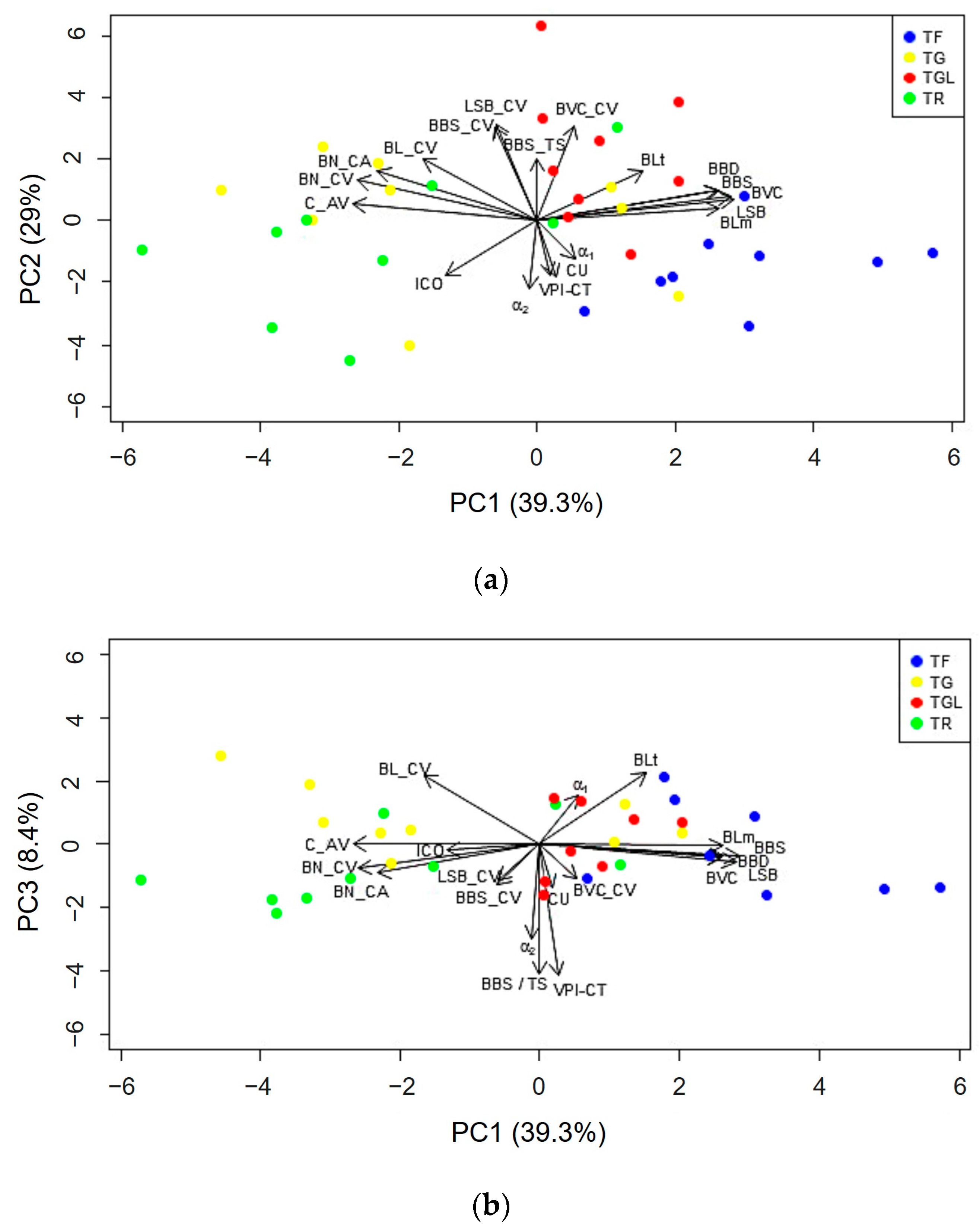
3.4. Principal Component Analysis to Discriminate the Cultivars

The PCA biplots (Figure 17) illustrate the distribution of the four hazelnut cultivars based on nineteen selected canopy morphological traits and indexes. The first four principal components (PCs) explain 82.3% of the total variance, with the first three PCs accounting for 76.7% (PC1: 39.3%, PC2: 29.0% and PC3: 8.4%).

PC1 primarily differentiates cultivars based on canopy and branch volume-related traits. Cultivars positioned towards the right (TGL and TF) exhibit more vigorous canopy structures and thicker branches, suggesting increased structural robustness. Conversely, cultivars like TG and TR, positioned towards the left, are associated with higher canopy openness and a more dispersed branching structure (BN_CA, C_AV, BL_CV, ICO). PC2 further refines these differences by capturing branch surface area and structural development. TGL, with higher PC2 values, is driven by traits such as LSB_CV, BBS_CV, and BVC_CV, which indicate a greater branch surface area and a more expansive canopy architecture. In contrast, TF, which is positioned towards lower PC2 values, is associated with α2, suggesting a more upright branching structure and a compact growth habit, which could be beneficial in high-density planting systems. A clearer distinction between TG and TR is observed along PC3, where VPI-CT, BBS_TS and α2 primarily contribute to their separation along this axis, related to a different canopy shape (VPI-CT and α2), and a less trunk vigour (BB_TS). Overall, PCA distinguishes cultivars based on morphological traits and morphological indexes, providing insights into their potential adaptability to different environmental conditions and management strategies.

The principal component analysis based on canopy morphological traits underlines that those selected traits obtained from the LiDAR point cloud can be used to classify hazelnut cultivars, which is useful for orchard with a mixture of cultivar, as well as for forests with a mixture of tree species [54].

3.5. Strength and Weakness of TLS in Fruit Tree Applications

TLS is a powerful and versatile tool for tree characterization and phenotyping, offering several significant advantages over traditional measurement techniques. It provides high precision and accuracy in capturing complex plant structures, including internal canopy features that are otherwise difficult to quantify [54]. The resulting point clouds constitute a permanent, high-resolution, three-dimensional digital record that can be revisited and reanalysed over time, unlike manual measurements which are typically non-repeatable and sensitive to operator variability.

In addition, TLS enables the automation of many processing steps (e.g., segmentation, canopy projection, and volumetric calculations), improving the objectivity, efficiency, and repeatability of morphological trait extraction. TLS data also support non-destructive measurements, reducing stress or damage to plants, and require fewer field operators compared to manual methods, which are often time-consuming, labor-intensive, and potentially invasive.

Nevertheless, some practical considerations must be acknowledged. In this study, the average acquisition time was approximately 9 min per scan, to achieve a resolution sufficient to capture even the internal canopy elements, both with (October 2023) and without foliage (March 2024). Each tree was scanned from four positions, arranged in a square around the plant to minimize occlusions and ensure complete structural coverage. While this setup provided rich and detailed data, it also resulted in large file sizes (about 150 MB per scan and several gigabytes for complete point cloud reconstructions, requiring dedicated workstations for efficient processing). Maintaining high point cloud resolution was essential for achieving the accuracy required for detailed structural analysis, especially during the leafless March 2024 survey. In this context, fine-scale features such as small branches and their diameters were only detectable with a dense point distribution. While reducing the resolution would decrease file size and might still allow for adequate measurement of certain features, such as canopy volume and area, it would compromise the identification and quantification of these finer traits, which are critical for morphological characterization.

The computational workflow, including registration, segmentation, and trait extraction, was partially automated using software tools and scripts available in commercial platforms (e.g., FARO Scene, Cyclone 3DR). However, more complex steps, such as main branch identification, still require manual input (Section 2.2). This mixed workflow, while robust, currently limits large-scale applicability due to processing time and user interaction.

To enhance the operational scalability of TLS, future developments could focus on the implementation of batch processing pipelines, greater automation, and the integration of open-source tools. In addition, emerging technologies such as SLAM-based LiDAR or mobile laser scanning systems (e.g., UAV-mounted or handheld platforms) represent promising alternatives. Although these systems typically offer lower spatial resolution, they substantially reduce both acquisition and processing times, which may be advantageous in large-scale orchard monitoring or breeding programs.

Future studies could also investigate the trade-offs between resolution and processing efficiency by testing downsampled point clouds. This would help define a minimum effective resolution that ensures analytical reliability while reducing data volume and computational load.

4. Conclusions

The three-dimensional data from TLS allowed for the definition of hazelnut plant traits by identifying of 18 morphological traits and by calculating 16 morphological indexes related to the tree vigour, tree growth habit and branching density, within an organized orchard. Then, the geometric models of canopy volume that best reproduce TLS estimates were identified, including the canopy volume derived from the “tree meshing script” in Cyclone 3DR.

Among the 18 morphological traits identified by using TLS, only six traits (BBD, BBS, BLm, BLt, BVC and LSB) proved suitable for defining tree vigour, while two traits (α1 and α2) were suitable for defining tree growth habit.

Among the 16 suggested morphological indexes, five traits (BBS_CV, BBS_TS, BN_CA, BN_CV and BVC_CV) proved suitable for defining branch density, three traits (BL_CV, C_AV and LSB_CV) were suitable for defining tree vigour, while three traits (ICO, CU and VPI—CT) were suitable for defining tree growth habit.

Two useful indexes were defined: CU (Canopy Uprightness) and ICO (Index of Canopy Opening).

These 19 descriptors allowed distinguishing the four studied hazelnut cultivars based on their growth habit; in particular, the cultivar TGL exhibited a growth habit quite different from that of the other ones. The TGL and TF cultivars exhibited more vigorous canopy structures and thicker branches, suggesting increased structural robustness. TGL is driven by traits such as LSB_CV, BBS_CV and BVC_CV, which indicate a greater branch surface area and a more expansive canopy architecture. In contrast, TF is associated with α2, suggesting a more upright branching structure and a compact growth habit, which could be beneficial in high-density planting systems. The TG and TR cultivars were associated with higher canopy openness and a more dispersed branching structure.

Moreover, among the morphological traits and indexes only BLt, BBS, BBD, VPI-CT and α1 were suitable for distinguishing the grafted plants from the own-rooted ones.

Since the LiDAR tree point cloud represents the above-ground parts of the tree, morphological traits and morphological indexes can be acquired from small trees, as well as from big ones.

In conclusion, the three-dimensional data from TLS have led to the definition of morphological traits of hazelnut plants and morphological indexes that can enable the objective description of different cultivars, which can be used by the International Union for the Protection of new Varieties of Plants (UPOV) to identify a new variety or to classify hazelnut cultivars within an orchard with a mixture of cultivars. In addition, morphological traits can be used to monitor the growth in young hazelnut trees.

The study will be completed by testing the morphological traits and morphological indices in other hazelnut cultivars characterized by different growth habits and vigour compared to those examined in this paper.

References

1. Sinoquet, H.; Bruno, A. The geometrical structure of plant canopies: Characterization and direct measurement methods. In Crop Structure and Light Microclimate; INRA Editions: Paris, France, 1993; pp. 131–158. [Google Scholar]
2. Valentini, N.; Caviglione, M.; Ponso, A.; Lovisolo, C.; Me, G. Physiological aspects of hazelnut trees grown in different training systems. Acta Hortic. 2009, 845, 233–238. [Google Scholar] [CrossRef]
3. Portarena, S.; Proietti, S.; Moscatello, S.; Zadra, C.; Cinosi, N.; Traini, C.; Farinelli, D. Effect of Tree Density on Yield and Fruit Quality of the Grafted Hazelnut Cultivar ‘Tonda Francescana®’. Foods 2024, 13, 3307. [Google Scholar] [CrossRef]
4. Costes, E.; Lauri, P.E.; Regnard, J.L. Analyzing fruit tree architecture: Implications for tree management and fruit production. Hortic. Rev. 2006, 32, 1–61. [Google Scholar]
5. Martinez-Guanter, J.; Ribeiro, Á.; Peteinatos, G.G.; Pérez-Ruiz, M.; Gerhards, R.; Bengochea-Guevara, J.M.; Machleb, J.; Andújar, D. Low-cost three-dimensional modeling of crop plants. Sensors 2019, 19, 2883. [Google Scholar] [CrossRef]
6. Walter, A.; Liebisch, F.; Hund, A. Plant phenotyping: From bean weighing to image analysis. Plant Methods 2015, 11, 14. [Google Scholar] [CrossRef] [PubMed]
7. Pace, R.; Masini, E.; Giuliarelli, D.; Biagiola, L.; Tomao, A.; Guidolotti, G.; Agrimi, M.; Portoghesi, L.; De Angelis, P.; Calfapietra, C. Tree measurements in the urban environment: Insights from traditional and digital field instruments to smartphone applications. Arboric. Urban For. 2022, 48, 113–123. [Google Scholar] [CrossRef]
8. Moorthy, I.; Miller, J.R.; Berni, J.A.J.; Zarco-Tejada, P.; Hu, B.; Chen, J. Field characterization of olive (Olea europaea L.) tree crown architecture using terrestrial laser scanning data. Agric. For. Meteorol. 2011, 151, 204–214. [Google Scholar] [CrossRef]
9. Lodolini, E.M.; de Iudicibus, A.; Lucchese, P.G.; Las Casas, G.; Torrisi, B.; Nicolosi, E.; Giuffrida, A.; Ferlito, F. Comparison of canopy architecture of five olive cultivars in a high-density planting system in Sicily. Agriculture 2023, 13, 1612. [Google Scholar] [CrossRef]
10. Costes, E.; Belouin, A.; Brouard, L.; Le Lezec, M. Development of young pear tree architecture and occurrence of first flowering: A varietal comparison. J. Hortic. Sci. Biotechnol. 2004, 79, 67–74. [Google Scholar]
11. Dewar, R.C. The Correlation between Plant Growth and Intercepted Radiation: An Interpretation in Terms of Optimal Plant Nitrogen Content. Ann. Bot. 1996, 78, 125–136. [Google Scholar] [CrossRef]
12. Hampson, C.R.; Azarenko, A.N.; Potter, J.R. Photosynthetic rate, flowering, and yield component alteration in hazelnut in response to different light environments. J. Am. Soc. Hortic. Sci. 1996, 121, 1103–1111. [Google Scholar] [CrossRef]
13. Ghosh, A.; Dey, K.; Das, S.; Dutta, P. Effect of Light on Flowering of Fruit Crops. Adv. Life Sci. 2016, 5, 2597–2603. [Google Scholar]
14. Singh, J.; Marboh Stone, E.; Singh, P.; Poojan, S. Light interception under different training system and high-density planting in fruit crops. J. Pharmacogn. Phytochem. 2020, 9, 611–616. [Google Scholar]
15. Dorji, Y.; Schuldt, B.; Neudam, L.; Dorji, R.; Middleby, K.; Isasa, E.; Korber, K.; Ammer, C.; Annighofer, P.; Seidel, D. Three-dimensional quantification of tree architecture from mobile laser scanning and geometry analysis. Trees 2021, 35, 1385–1398. [Google Scholar] [CrossRef]
16. Tombesi, S.; Farinelli, D. Modelling of pruning technique effects on branch architecture and subsequent year shoot flowering in hazelnut. Acta Hortic. 2017, 1160, 141–144. [Google Scholar] [CrossRef]
17. Costes, E.; Crespel, L.; Denoyes, B.; Morel, P.; Demene, M.N.; Lauri, P.E.; Wenden, B. Bud structure, position and fate generate various branching patterns along shoots of closely related Rosaceae species: A review. Front. Plant Sci. 2014, 5, 666. [Google Scholar] [CrossRef]
18. Montesinos, Á.; Thorp, G.; Grimplet, J.; Rubio-Cabetas, M.J. Phenotyping almond orchards for architectural traits influenced by rootstock choice. Horticulturae 2021, 7, 159. [Google Scholar] [CrossRef]
19. Grisafi, F.; Tombesi, S.; Farinelli, D.; Boudon, F.; Durand, J.B.; Costes, E. Analysing the architecture of Corylus avellana and parametrizing L. Hazelnut FSPM. In Proceedings of the 10th International Conference on Functional-Structural Plant Models (FSPM2023), Berlin, Germany, 27–31 March 2023. [Google Scholar]
20. Grisafi, F.; Farinelli, D.; Costes, E.; Boudon, F.; Durand, J.B.; Tombesi, S. Analysis of bud and sylleptic shoot distribution along one-year-old shoots of hazelnut (Corylus avellana). Acta Hortic. 2023, 1379, 283–290. [Google Scholar] [CrossRef]
21. Grisafi, F.; Farinelli, D.; Costes, E.; Boudon, F.; Durand, J.B.; Tombesi, S. Architecture and yield relationship in hazelnut tree. Acta Hortic. 2023, 1366, 331–336. [Google Scholar] [CrossRef]
22. Grisafi, F.; Tombesi, S.; Farinelli, D.; Costes, E.; Durand, J.B.; Boudon, F. Modelling the architecture of hazelnut (Corylus avellana) Tonda di Giffoni over two successive years. Silico Plants 2024, 6, diae004. [Google Scholar] [CrossRef]
23. Vandendaele, B.; Martin-Ducup, O.; Fournier, R.A.; Pelletier, G.; Lejeune, P. Mobile Laser Scanning for Estimating Tree Structural Attributes in a Temperate Hardwood Forest. Remote Sens. 2022, 14, 4522. [Google Scholar] [CrossRef]
24. Holopainen, M.; Kankare, V.; Vastaranta, M.; Liang, X.; Lin, Y.; Vaaja, M.; Yu, X.; Hyyppä, J.; Hyyppä, H.; Kaartinen, H.; et al. Tree mapping using airborne, terrestrial and mobile laser scanning–A case study in a heterogeneous urban forest. Urban For. Urban Green. 2013, 12, 546–553. [Google Scholar] [CrossRef]
25. Stal, C.; Verbeurgt, J.; De Sloover, L.; De Wulf, A. Assessment of handheld mobile terrestrial laser scanning for estimating tree parameters. J. For. Res. 2021, 32, 1503–1513. [Google Scholar] [CrossRef]
26. Estornell, J.; Hadas, E.; Martí, J.; López-Cortés, I. Tree extraction and estimation of walnut structure parameters using airborne LiDAR data. Int. J. Appl. Earth Obs. Geoinf. 2021, 96, 102273. [Google Scholar] [CrossRef]
27. Okura, F. 3D modeling and reconstruction of plants and trees: A cross-cutting review across computer graphics, vision, and plant phenotyping. Breed Sci. 2022, 72, 31–47. [Google Scholar] [CrossRef]
28. Zhu, Z.H.; Christoph, K.; Nölke, N. Assessing tree crown volume—A review. Forestry 2021, 94, 18–35. [Google Scholar] [CrossRef]
29. Hopkinson, C.; Chasmer, L.; Young-Pow, C.; Treitz, P. Assessing Forest metrics with a ground-based scanning LIDAR. Can. J. For. Res. 2004, 34, 573–583. [Google Scholar] [CrossRef]
30. Rutzinger, M.; Pratihast, A.K.; Oude Elberink, S.; Vosselman, G. Detection and modelling of 3D trees from mobile laser scanning data. Int. Arch. Photogramm. Remote Sens. Spat. Inf. Sci. 2010, 38, 520–525. [Google Scholar]
31. Lin, Y.; Herold, M. Tree species classification based on explicit tree structure feature parameters derived from static terrestrial laser scanning data. Agric. For. Meteorol. 2016, 216, 105–114. [Google Scholar] [CrossRef]
32. Reich, K.F.; Kunz, M.; von Oheimb, G. A new index of forest structural heterogeneity using tree architectural attributes measured by terrestrial laser scanning. Ecol. Indic. 2021, 133, 108412. [Google Scholar] [CrossRef]
33. Brigante, R.; Calisti, R.; Marconi, L.; Proietti, P.; Radicioni, F.; Vinci, A. GNSS NRTK-UAV photogrammetry and LiDAR point clouds for geometric features extraction of olive orchard. In Proceedings of the 2024 IEEE International Workshop on Metrology for Agriculture and Forestry (MetroAgriFor), Padua, Italy, 29–31 October 2024; pp. 563–568. [Google Scholar] [CrossRef]
34. Bogdanovich, E.; Perez-Priego, O.; El-Madany, T.S.; Guderle, M.; Pacheco-Labrador, J.; Levick, S.R.; Moreno, G.; Carrara, A.; Pilar Martín, M.; Migliavacca, M. Using terrestrial laser scanning for characterizing tree structural parameters and their changes under different management in a Mediterranean open woodland. For. Ecol. Manag. 2021, 486, 118945. [Google Scholar] [CrossRef]
35. Vinci, A.; Brigante, R.; Traini, C.; Farinelli, D. Geometrical Characterization of Hazelnut Trees in an Intensive Orchard by an Unmanned Aerial Vehicle (UAV) for Precision Agriculture Applications. Remote Sens. 2023, 15, 541. [Google Scholar] [CrossRef]
36. McGaughey, R.J.; Kruper, A.; Bobsin, C.R.; Bormann, B.T. Tree Species Classification Based on Upper Crown Morphology Captured by Uncrewed Aircraft System Lidar Data. Remote Sens. 2024, 16, 603. [Google Scholar] [CrossRef]
37. Bioversity; FAO; CIHEAM. Descriptors for Hazelnut (Corylus avellana L.); Bioversity International: Rome, Italy; Food and Agriculture Organization of the United Nations: Rome, Italy; International Centre for Advanced Mediterranean Agronomic Studies: Zaragoza, Spain, 2008. [Google Scholar]
38. UPOV. Available online: https://www.upov.int/meetings/en/doc_details.jsp?meeting_id=60592&doc_id=541353 (accessed on 20 March 2025).
39. Coupel-Ledru, A.; Pallas, B.; Delalande, M.; Boudon, F.; Carrié, E.; Martinez, S.; Regnard, J.L.; Costes, E. Multi-scale high-throughput phenotyping of apple architectural and functional traits in orchard reveals genotypic variability under contrasted watering regimes. Hortic. Res. 2019, 6, 52. [Google Scholar] [CrossRef]
40. Traini, C.; Facchin, S.L.; Brigante, R.; Vinci, A.; Persichetti, S.; Meneghini, M.; Micheli, M.; Famiani, F.; Portarena, S.; Dradi, G.; et al. Field performance of grafted, micropropagated, and own-rooted plants of three Italian hazelnut cultivars during the initial four seasons of development. Front. Plant Sci. 2024, 15, 1412170. [Google Scholar] [CrossRef]
41. Portarena, S.; Gavrichkova, O.; Brugnoli, E.; Battistelli, A.; Proietti, S.; Moscatello, S.; Famiani, F.; Tombesi, S.; Zadra, C.; Farinelli, D. Carbon allocation strategies and water uptake in young grafted and own-rooted hazelnut (Corylus avellana L.). Tree Physiol. 2022, 42, 939–957. [Google Scholar] [CrossRef]
42. Scorza, R.; Lightner, G.W.; Liverani, A. The pillar peach tree and growth habit analysis of compact × pillar progeny. J. Am. Soc. Hortic. Sci. 1989, 114, 991–995. [Google Scholar] [CrossRef]
43. Pretzsch, H. Canopy space filling and tree crown morphology in mixed-species stands compared with monocultures. For. Ecol. Manag. 2014, 327, 251–264. [Google Scholar] [CrossRef]
44. Owen, H.J.F.; Lines, E.R. Common field measures and geometric assumptions of tree shape produce consistently biased estimates of tree and canopy structure in mixed Mediterranean forests. Ecol. Indic. 2024, 165, 112219. [Google Scholar] [CrossRef]
45. Asante, W.A.; Ahoma, G.; Gyampoh, B.; Kyereh, B.; Asare, R. Upper canopy tree crown architecture and its implications for shade in cocoa agroforestry systems in the western region of Ghana. Trees For. People 2021, 5, 100100. [Google Scholar] [CrossRef]
46. Farinelli, D.; Portarena, S.; da Silva Fernandes, D.; Traini, C.; Menegazzo da Silva, G.; Costa da Silva, E.; Ferreira da Veiga, J.; Pollegioni, P.; Villa, F. Variability of Fruit Quality among 103 Acerola (Malpighia emarginata D.C.) Phenotypes from the Subtropical Region of Brazil. Agriculture 2021, 11, 1078. [Google Scholar] [CrossRef]
47. Leposavić, A.; Ružić, D.; Karaklajić-Stajić, Z.; Cerović, R.; Vujović, T.; Žurawicz, E.; Mitrovic, O. Field performance of micropropagated Rubus species. Acta Sci. Pol. Hortorum Cultus 2016, 15, 3–14. [Google Scholar]
48. Tarsha Kurdi, F.; Gharineiat, Z.; Lewandowicz, E.; Shan, J. Modeling the Geometry of Tree Trunks Using LiDAR Data. Forests 2024, 15, 368. [Google Scholar] [CrossRef]
49. Fish, H.; Lieffers, V.J.; Silins, U.; Hall, R.J. Crown shyness in lodgepole pine stands of varying stand height, density, and site index in the upper foothills of Alberta. Can. J. For. Res. 2006, 36, 2104–2111. [Google Scholar] [CrossRef]
50. Hashimoto, R. Canopy development in young sugi (Cryptomeria japonica) stands in relation to changes with age in crown morphology and structure. Tree Physiol. 1991, 8, 129–143. [Google Scholar] [CrossRef]
51. Jatzek, V.A.; Menecheli Filho, H.; Rocha, G.N.; Silva, O.J.; Rodriguez, L.C.E.; Paula, R.C.D.; Silva, P.H.M.D. Comparative assessment of LiDAR and conventional methods in evaluating genetic parameters of eucalypt progeny trials. Crop Breed. Appl. Biotechnol. 2025, 25, e50382516. [Google Scholar] [CrossRef]
52. Farinelli, D.; Boco, M.; Tombesi, A. Productive and organoleptic evaluation of new hazelnut crosses. Acta Hortic. 2009, 845, 651–656. [Google Scholar] [CrossRef]
53. Walter, J.D.; Edwards, J.; McDonald, G.; Kuchel, H. Estimating biomass and canopy height with LiDAR for field crop breeding. Front. Plant Sci. 2019, 10, 1145. [Google Scholar] [CrossRef]
54. Lindberg, E.; Johan, H. Individual tree crown methods for 3D data from remote sensing. Curr. For. Rep. 2017, 3, 19–31. [Google Scholar] [CrossRef]
Figure 1. Workflow of the methodological approach; S1 refers to the survey carried out in October and S2 to the one conducted in March.
Agriculture 15 01251 g001
Figure 2. Location map of the study area—central point coordinates: latitude 42°58′20.0″ N, longitude 12°24′11.1″ E, in the WGS84 reference system (a); planimetric layout inside the red square (b) and photographic overview (c) of the hazelnut orchard under study.
Agriculture 15 01251 g002
Figure 3. Laser scanning surveys: October 2023 (a) and March 2024 (b).
Agriculture 15 01251 g003
Figure 4. Point cloud processing with Scene ((a): October 2023; (b): March 2024) and Cyclone 3DR ((c): October 2023; (d): March 2024). The red dots indicate the scan positions during the survey.
Agriculture 15 01251 g004
Figure 5. Geometrical features extracted from the October 2023 survey: canopy height and canopy area (a); canopy volume estimated by shell (b); and tree meshing script (c).
Agriculture 15 01251 g005
Figure 6. Examples of canopy structures: (a) asymmetrical, (b) symmetrical, (c) sparse and (d) dense. In (a,b), the red dashed line represents the circumference with a diameter (bmean) equal to the average of bmin and bmax.
Agriculture 15 01251 g006
Figure 7. Geometrical features extracted from the March 2024 survey: trunk circumference (a); length and radius of the branches (b); branch angles (c).
Agriculture 15 01251 g007
Figure 8. Canopy shape and distance between principal branches in a closed (a,b) and an opened (c,d) branching structure.
Agriculture 15 01251 g008
Figure 9. Canopy shape compared to the ellipsoid (a), cylinder (b), cone trunk (c) and parallelepiped (d) shapes.
Agriculture 15 01251 g009
Figure 10. Tree growth habit: (a) erect; (b) semi-erect; (c) spreading.
Agriculture 15 01251 g010
Figure 11. Tree growth habit distribution (erect when the angle between trunk and branch (α1) is < 35°; semi-erect between 35° and 55°; spreading between 55° and 75°; and drooping when the angle is >75°), expressed as a percentage per each class. Different letters indicate significant (p < 0.05) differences among cultivars per each class of distribution.
Agriculture 15 01251 g011
Figure 12. Tree growth habit discriminated by α2: (a) erect (TGL); (b) semi-erect (TF).
Agriculture 15 01251 g012
Figure 13. Box plot of the differences between canopy volume obtained through manual measurements and those derived from the laser point clouds (CVSHELL and CVMESH). Whiskers (error bars) above and below the box indicate the 90th and 10th percentiles. The horizontal line shows the median value.
Agriculture 15 01251 g013
Figure 14. Canopy shape discriminated by VPI-CT: TGL (a) and TG (b) show a shape more similar to a cone trunk compared to TF (c) and TR (d).
Agriculture 15 01251 g014
Figure 15. Canopy shape discriminated by VPI-CT: grafted (a); micropropagated (b); and own-rooted (c).
Agriculture 15 01251 g015
Figure 16. Index of Canopy Opening (ICO) distribution as plant per class (%/tot), with the following classes: canopy with close branches, when ICO < 0.35; almost close branches, when ICO = 0.35–0.45; almost distant branches, when ICO = 0.45–0.50; and distant branches, when ICO > 0.55. In each class, different letters indicate significant (p < 0.05) differences among the cultivars per each distribution class.
Agriculture 15 01251 g016
Figure 17. Scatter plots of PCA scores for four hazelnut cultivars based on canopy morphological traits. Biplots show the relationships between PC1 and PC2 (a) and between PC1 and PC3 (b).
Agriculture 15 01251 g017