An Innovative Inversion Method of Potato Canopy Chlorophyll Content Based on the AFFS Algorithm and the CDE-EHO-GBM Model

Abstract

Chlorophyll content is an important indicator for estimating potato growth. However, there are still some research gaps in the inversion of canopy chlorophyll content using unmanned aerial vehicle (UAV) remote sensing. For example, it faces limitations of the growth cycle, low parameter accuracy, and single feature selection, and there is a lack of efficient and precise systematic research methods. In this study, an improved Adaptive-Forward Feature Selection (AFFS) algorithm was developed by combining remote sensing data and measured data to optimize the input Vegetation Index (VI) variables. Gradient Boosting Machine (GBM) model parameters were optimized using a hybrid strategy improved Elephant Herd Optimization (EHO) algorithm (CDE-EHO) that combines Differential Evolution (DE) and Cauchy Mutation (CM). The CDE-EHO method optimizes the GBM model, achieving maximum accuracy, according to the testing results. The optimal coefficients of determination (R²) values of the prediction set are 0.663, 0.683, and 0.906, respectively, the Root Mean Squared Error (RMSE) values are 2.673, 3.218, and 2.480, respectively, and the Mean Absolute Error (MAE) values are 2.052, 2.732, and 1.928, respectively, during the seedling stage, tuber expansion stage and cross-growth stage. This approach has significantly enhanced the inversion model’s prediction performance as compared to earlier research. The chlorophyll content in the potato canopy has been accurately extracted in this work, offering fresh perspectives and sources for further research in this area.

1. Introduction

Potatoes, being a staple food crop both in China and globally, have their production levels and quality intricately associated with not only food security but also the development of other industries [1]. Chlorophyll, an essential element in the biological processes of potato plants, plays a crucial role as the primary pigment in photosynthesis, participating in light energy absorption, transmission, and conversion. Moreover, it determines the efficacy of photosynthetic processes and serves as an index reflecting the plant’s nutritional state [2]. To accurately assess the growth condition of potato plants, optimize fertilization strategies, and predict yields, obtaining precise data regarding the chlorophyll content within the potato canopy is of utmost significance [3].

Conventional techniques like spectrophotometry and high-performance liquid chromatography (HPLC) [4] require laborious, time-consuming procedures that damage leaves and cannot estimate chlorophyll content over large areas. Because of its cost-effectiveness, real-time capability, and operational flexibility, UAV multispectral remote sensing technology is expanding in use [5]. The SPAD-502 handheld chlorophyll meter measures the Soil and Plant Analyzer Development (SPAD) values of the potato canopy in the field precisely [6]. Measured SPAD values can be utilized in place of chlorophyll content because of the study’s excellent association between chlorophyll concentration and SPAD values. Integrating unmanned aerial vehicle (UAV) remote sensing techniques with in situ measured SPAD data represents a crucial component within the domain of smart agriculture [7]. Yang et al. [8] used UAV multispectral data to calculate the chlorophyll content in potatoes and constructed a model based on k-nearest neighbor (KNN), light gradient boosting machine (Light-GBM), support vector machine (SVM), and stacked generalization model (SGM). The model had a root-mean-square error (RMSE) of 0.511 and a coefficient of determination (R²) of up to 0.739. Mohamad et al. [9] created a new mathematical model based on remote sensing data and techniques by using high temporal resolution and low spatial resolution images. Based on the new mathematical model, a new computerized intelligent system for proper decision making was implemented. Tian et al. [10] took cotton multi-fertility pictures using a UAV fitted with a multispectral camera. They then segmented the images using techniques such as mixed spectral analysis of multiple end elements (MSE-MSA). The findings indicated that the support vector regression (SVR) model had the highest efficiency in inverting the cotton chlorophyll content, with R² values of 0.810, 0.778, and 0.697. Manal et al. [11] estimated the plant chlorophyll content from high-resolution images by applying the correlation vector machine (CVM) in combination with cross-validation and the backward elimination approach (BEA). The RMSE was 5.31 μg/cm², and the efficiency was 0.76. To obtain more effective findings, researchers must precisely control the location and conditions of ground sampling and improve its accuracy. Combining a machine learning system with high-resolution spectral information collected by a multispectral sensor mounted on a UAV, Gaurav et al. [12] discovered that a convolutional neural network (CNN) model grounded in deep learning is highly effective in inverting the chlorophyll content. Nevertheless, the intricate and multi-parameter structure of deep learning models, like CNN, may result in inadequate interpretability.

The rapid advancement of remote sensing technology has led to the ability to calculate the content of chlorophyll utilizing multispectral data [13]. The vegetation index (VI), which serves as a crucial link between remotely sensed spectral data and plant physiological traits, plays an increasingly important role in crop growth monitoring [14]. Leveraging VI, an optimized composite parameter, can streamline the processing workflow. Nevertheless, different VIs exhibit varying degrees of sensitivity to chlorophyll content. Therefore, identifying and applying appropriate VIs is a key factor in improving estimation accuracy and model training effectiveness [15]. To increase inversion accuracy, Guo et al. [16] employed synergistic inversion of leaf area index (LAI) and leaf chlorophyll content (LCC), which produced R² = 0.45 and RMSE = 32.71 μg/cm² for LCC and R² = 0.60 and RMSE = 2.80 μg/cm² for LAI. For their inversion study of green leaf area index (LAI), total chlorophyll content (TC-ab), and other metrics, Rasmus et al. [17] combined VI and physically based methods. They calculated root mean square (RMS) deviations by comparing estimates with field measurements, yielding values of 0.62 for barley, 0.46 for wheat, and 0.63 for deciduous forests. This study has limitations in assessing other environments and species composition. The Normalized Area Vegetation Index (NAVI), which Facundo et al. [18] proposed as a method to calculate the quantity of chlorophyll using remote sensing data, demonstrated a good linear correlation with the Normalized Area for Chlorophyll (NAOC) index, with a value that is 0.97 or higher. This provides an innovative and highly efficient means of estimating the chlorophyll quantity within multispectral remote-sensing data.

Machine learning (ML) models demonstrate significant potential in improving both the quality and yield efficiency of agricultural production [19,20,21]. ML models analyze non-linear relationships between chlorophyll concentration and multiple factors. Moreover, they exhibit remarkable generalization capabilities [22]. By leveraging remote sensing technologies and other relevant tools, the pretrained model can be employed to conduct dynamic monitoring of vegetation and promptly estimate its chlorophyll content over a broad area in real-time. By merging VI and ML models, Syed et al. [23] assessed the content of chlorophyll in wheat leaves by employing the random forest method. The results demonstrated that adding VI as an input variable enhanced the model’s accuracy, reducing the RMSE to between 3.62 and 3.91 μg·cm⁻². Pan et al. [24] constructed an SPAD inversion model for summer maize by correlating the sensitive characteristics of chlorophyll content using multiple linear regression (MLR) and partial least squares regression (PLSR) models. The results showed that the MLR model under a single data source was the best. The RF model under multiple data sources was the best, and the R² and RMSE of this model were 0.9114 and 2.3955, respectively. Zhao et al. [25] created a semi-empirically accelerated three-dimensional radiative transfer model (SE-A3DRTM), which was integrated with a machine learning model to carry out an inversion investigation of chlorophyll concentration. They trained the models with PROSAIL-generated datasets, and the results showed that all models trained using SE-A3DRTM outperformed PROSAIL. Li et al. [26] combined multispectral (MS) technology with four machine learning models, including a BP neural network (BP), to monitor the chlorophyll content of maize at the whole growth stage. The results showed that the SVR model combined with MS-RGB fusion feature data had the highest accuracy with an R² of 0.896, which could significantly improve the accuracy of chlorophyll content monitoring.

ML models demonstrate remarkable adaptability to a wide array of datasets and diverse problem scenarios. Additionally, they are able to quantitatively elucidate the relationship between crops and the chlorophyll content present therein [27]. Nevertheless, several limitations persist. For instance, the model exhibits sensitivity to parameter variations, a proclivity for overfitting, and a tendency to converge to local optimal solutions [28]. For example, traditional gradient descent algorithms are simple but prone to local optima, and heuristic optimization algorithms have been developed to overcome this shortcoming. The artificial intelligence algorithm used in this study has a strong global search capability over a large parameter space. The intelligent algorithm incorporates randomness and diversity, which prevents the program from converging to local solutions and succumbing to overfitting [29]. Meysam et al. [30] created a constrained learning machine model for the calculation of chlorophyll content and used a heuristic optimization integrated bat algorithm (Bat-ELM) to tune the parameters of this learning model. The results of the study showed that the Bat-ELM model outperformed the other models with a 20.7% improvement in model performance. To estimate the amount of chlorophyll during date leaf mite infection, Lu et al. [31] suggested an extreme learning machine (ELM) based on the particle swarm optimizer (PSO). With a 0.856 R² and a 0.796 RMSE, the precision of the improved PSO-ELM model was noticeably higher. Wu et al. [32] suggested optimizing the support vector regression (SVR) approach to predict chlorophyll content by combining the Adaptive Ant Colony Exhaustive Optimization (A-ACEO) algorithm with the Genetic approach (GA). The findings indicated a significant enhancement in accuracy, presenting a 0.0345 RMSE and a 0.9617 R² value. The intelligent optimization approach often solves the model accuracy issue to a certain degree, but overfitting and local optimal solution issues persist. In response to these problems, this study introduced two improved algorithms to optimize the Elephant Herd Optimization (EHO) Algorithm and achieved good results. The EHO algorithm can effectively simulate the complex interaction relationships in the chlorophyll content inversion model, thus significantly enhancing the model’s prediction performance. Other techniques, such as grid search algorithms, lack adaptability to dynamic changes in the model and can only be searched in a fixed parameter grid, which is likely to fall into local optimal solutions.

In conclusion, this study used the Xufeng potato experimental base in Wuchuan County, Hohhot City, as the study region. By integrating UAV remote sensing technology with collected ground data, the SPAD values of the potato canopy were inverted. This paper’s primary research project is: (1) VI is built using canopy reflectance taken from UAV photos, and the adaptive mechanism is added to the FFS algorithm to adjust the weights dynamically and enhance the vegetation feature selection. (2) The selected VIs are used as inputs to compare the precision and efficacy of different models. (3) To avoid overfitting, the GBM model’s parameters are optimized using the EHO approach. It has the capacity to search globally for a better combination of the inverse model’s hyperparameters. (4) In order to maximize the population information interactions and improve both local and global search capabilities, the Differential Evolutionary method (DE) and the Cauchy Mutation Algorithm (CM) are used to improve the EHO optimization method.

2. Materials and Methods

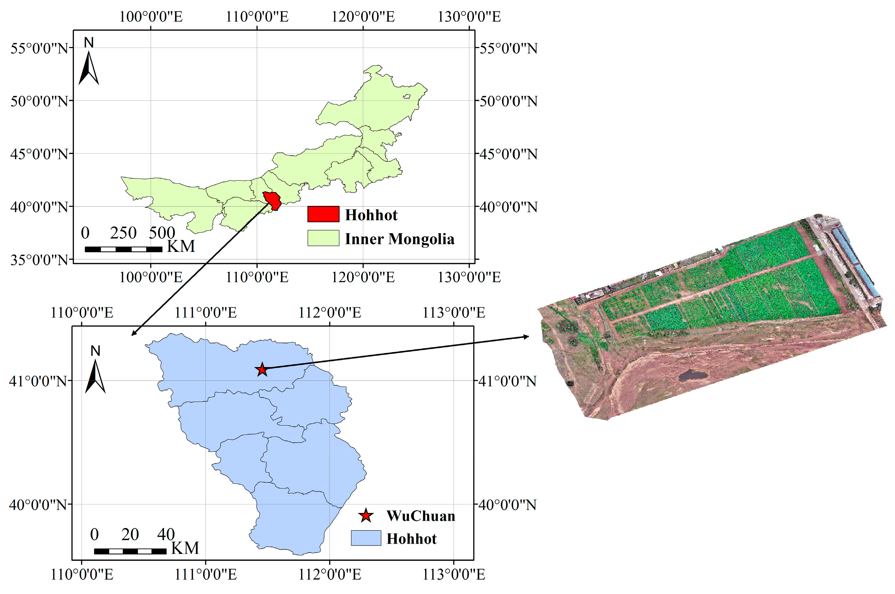
2.1. Study Area

The study location served as the Xufeng Seed Industry’s potato-planting base in Wuchuan County, Hohhot City (shown in Figure 1). This facility is situated north of Hohhot City in the central region of the Inner Mongolia Autonomous Region. The coordinates of this location are 41°9′36” N, 111°36′10” E. Wuchuan County is characterized by a mesothermal continental monsoon climate. In such a climate, there are significant disparities between daytime and nighttime temperatures, as well as between winter and summer temperatures. The average elevation is between 1500 and 2000 m, the average temperature is 4.2 °C each year, and there is 360–366 mm of precipitation annually. Throughout the year, there is an abundance of light resources and enough sunshine, which supports agricultural photosynthesis.

2.2. Data Set

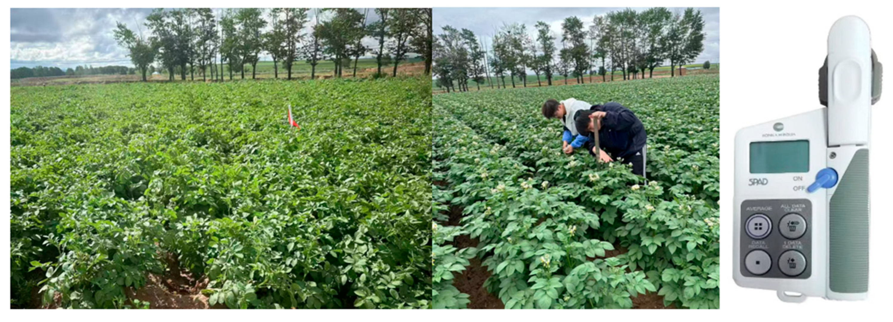
2.2.1. Measured Canopy SPAD Value Data

We gathered the study’s canopy SPAD value data on 10 July 2024 (the seedling stage) and 12 August 2024 (the tuber expansion stage) at the Xufeng potato-planting base in Dazhoupu Village, Wuchuan County. To ensure the experiment’s rigor and avoid data duplication, we collected data twice in each growth period. The data from these two collections were used for experiments in the single-fertile growth phase and the cross-growth phase, respectively. The canopy SPAD value can be a useful indicator of the plant’s general physio-logical state and growth circumstances. Thus, the SPAD-502 handheld chlorophyll meter was utilized to determine the canopy’s SPAD value. We calculated the canopy SPAD value by averaging measurements from ten randomly selected leaf flesh spots, excluding veins. The study area was divided into 16 different plots, each corresponding to one of the 16 potato varieties in the trial. Each plot measured 100 m × 20 m and was spatially separated to avoid interference between varieties. We used uniform sampling to record average values of approximately 10 sample points in each region, and a total of 162 pieces of canopy SPAD value data were collected. The SPAD-502 handheld chlorophyll meter and the gathered field photos during the seedling and tuber expansion stages are displayed in Figure 2.

2.2.2. Remote Sensing Imagery Data from UAV

This study used a DJI Mavic 3M UAV (DJI, Shenzhen, China), as illustrated in Figure 3. The UAV is equipped with four multispectral sensors, which specifically correspond to the near-infrared band, the red band, the green band, and the red-edge band. It exhibits a net weight of approximately 958 g, a maximum weight of 1050 g at takeoff, and a maximum height of 6000 m during flight. The UAV imagery employed in this study was acquired on 10 July 2024, from 8:30 to 11:30 a.m., and on 12 August 2024, from 9:00 to 12:00 p.m. We collected UAV imagery on each specified day. With a solar altitude angle of roughly 50° and low humidity of roughly 40%, the data collection day was clear and less overcast, making it ideal for the UAV to precisely capture multispectral photos.

Table 1. Parameters settings for drone flight.

Parameters	Specific Value
Flight velocity	5 m/s
Flight altitude	30 m
Lateral overlap rate	70%
Longitudinal overlap rate	80%
Wavelength range of green light	560 nm ± 16 nm
Wavelength range of red light	650 nm ± 16 nm
Wavelength range of red edge band	730 nm ± 16 nm
Wavelength range of near-infrared band	860 nm ± 26 nm

displays the pertinent UAV parameter settings.

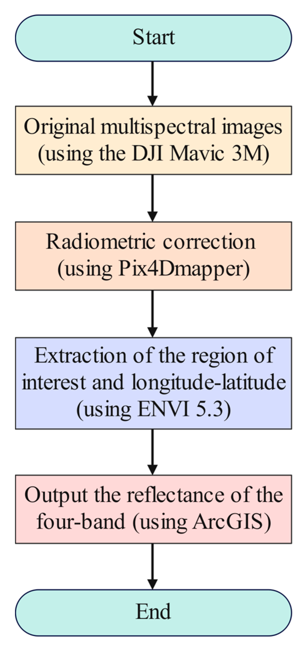
2.2.3. Preprocessing of Remote Sensing Data

After the drone’s flight mission, we processed and reconstructed the acquired images through the DJI Smart Agriculture Platform (DJI SF Platform, available at https://ag.dji.com/cn/smartfarm-web, accessed on 2 September 2024) to generate the original multispectral images. Then, we radiometrically calibrated the original multispectral images with Pix4Dmapper software (version 4.5.6) to produce orthophotos. In this study, we extracted the longitude and latitude of the measurement sites with the help of the ENVI 5.3 software (version 5.3.1). During the real data collection process, we set up red flags at each sampling site to mark the extraction locations. The calibrated orthophoto and extracted latitude and longitude data were entered into the ArcGIS application (ArcGIS Pro 3.3). We obtained reflectance values in the red, green, red-edge, and near-infrared bands, after which we constructed VIs for subsequent testing. Figure 4 depicts the UAV image data preparation path.

2.3. Construct Feature Variables

Vegetation exhibits distinct reflectance characteristics across multiple bands. Moreover, in remote-sensing images, the reflectance of vegetation can be affected by atmospheric scattering and absorption. These factors impede the accurate acquisition of vegetation-related information. By performing specific operations on the reflectance values of different bands, the spectral signatures of vegetation can be enhanced by the VIs, which can also decrease or even eliminate the effects caused by the previously described components.

Table 2. Twenty VIs utilized for SPAD value inversion in this study.

Vegetation Index	Name	Formula	References
GRVI	Green–Red Vegetation Index	GRVI = (G-R)/(G + R)	[33]
MCARI	Modified Chlorophyll Absorption Ratio Index	MCARI = (RE − R) − (0.2 × (RE − G)) × (RE/R)	[34]
DVI	Difference Vegetation Index	DVI = NIR − R	[35]
MTVI	Modified Tri-angular Vegetation Index	MTVI = 1.5 × (1.2 × (RE − G) − 2.1 × (R − G))	[36]
WDRVI	Wide Dynamic Range Vegetation Index	WDRVI = (0.12 × NIR − R)/(0.12 × NIR + R)	[37]
EVI2	Two-band Enhanced Vegetation Index	EVI2 = 2.5 × (NIR − R)/(NIR + 2.4 × R + 1)	[38]
RECI	Red Edge Chlorophyll Index	RECI = (NIR/RE) − 1	[39]
GCI	Green Chlorophyll Index	GCI = (NIR/G) − 1	[40]
NDVI	Normalized Difference Vegetation Index	NDVI = (NIR − R)/(NIR + R)	[41]
GNDVI	Green Normalized Difference Vegetation Index	GNDVI = (NIR − G)/(NIR + G)	[42]
RVI	Ratio Vegetation Index	RVI = NIR/R	[43]
NDGI	Normalized Difference Green Index	NDGI = (RE − G)/(RE +G)	[34]
MSRI	Modified Simple Ratio Index	MSR = (NIR/R − 1)/(NIR/R + 1)	[44]
OSAVI	Optimized Soil-Adjusted Vegetation Index	OSAVI = (NIR − R)/(NIR + R + 0.16)	[45]
SRI	Simple Ratio Index	SR = NIR/RE	[46]
NDRE	Normalized Difference Red Edge Index	NDRE = (NIR − RE)/(NIR + RE)	[47]
NLI	Nonlinear Vegetation Index	NLI = (NIR × NIR − R)/(NIR × NIR + R)	[48]
TVI	Triangular Vegetation Index	TVI = 0.5 × (120 × (NIR − RE) − 200 × (R − RE))	[49]
GRRI	Green–Red Edge Ratio Index	GRRI = G/RE	[50]
RNVI	Red-Edge Normalized Vegetation Index	RNVI = (RE − R)/(RE + R)	[51]

presents the 20 VIs formulated in this research.

2.4. Feature Selection Methods

If redundant VIs are incorporated, the performance of the model will deteriorate, while its training time and computational cost will escalate. Selecting appropriate VIs retains the most valuable features and removes superfluous data that contribute little to the model. This procedure improves the model’s precision and training effectiveness. In this research, we employed the following algorithms to select VIs.

2.4.1. Competitive Adaptive Reweighted Sampling Algorithm

Competitive Adaptive Reweighted Sampling (CARS) algorithm [52] simulates the “the fittest survive“ principle in biological evolution by using Monte Carlo sampling and exponential decay weights. A set of variables capable of most effectively accounting for the target variable is selected through adaptive variable-weight adjustment and multiple random sampling procedures. Equation (1) provides the formula for calculating the weight $w_i$ of the ith vegetation index:

$$w_i={\displaystyle \frac{\left|b_i\right|}{{\displaystyle \sum _{j=1}^m\left|b_i\right|}}}$$

(1)

among them, $b_i$ is the regression value of the ith vegetation index in the Partial Least Squares (PLS) model, and m is the quantity of VIs that are engaged in the model-building process.

For each sample, we built a PLS model with the retained VIs and compute the root mean square error of cross-validation (RMSECV). The formula for RMSECV is shown in Equation (2):

$$RMSECV=\sqrt{{\displaystyle \frac{{\displaystyle \sum _{i=1}^m{(y_i-{\widehat{y}}_i)}^2}}{m}}}$$

(2)

among them, $m$ is the cross-validation sample count, $y_i$ is the ith sample’s real amount, and ${\widehat{y}}_i$ is the ith sample’s anticipated amount obtained from the model established based on the currently screened VI subset. The CARS algorithm determines the optimal VI subset by continuously sampling with the aim of minimizing the RMSECV. Subsequent models then used the optimal VI subset to predict chlorophyll content.

2.4.2. Fast Forward Selection Algorithm

The core principle of the Fast Forward Selection (FFS) algorithm [53] is to start with an empty feature subset. In each iteration, it greedily selects a Vegetation Index (VI) that can optimize the objective function and then adds it to the current subset. It progresses towards the predefined stopping condition by making sequential choices. Through this process, it effectively reduces the dimensionality of the data, thereby enhancing the accuracy and efficiency of the model.

Suppose there are initially $n$ VIs, denoted as the set $V=\{v_1,v_2,\dots ,v_n\}$. The given value of n under the present research is 20. The initial VI subset $S$ is set as an empty set. To assess the quality of the VI subset $S$, a target function $J(S)$ is defined. This function is connected to the discrepancy between the real and anticipated outcomes in this study. After adding the VI $v_i$ to $S$, determine the total of squared errors $J(S\cup \{v_i\})$ for each Vegetation Index A that is not in the current subset $S$. Equation (3) is its calculation formula:

$$J(S\cup \{v_i\})={\displaystyle \sum _{j=1}^m{(y_j-({\widehat{\beta }}_0+{\displaystyle {\sum }_{v_k\in S\cup \left\{v_i\right\}}{\widehat{\beta }}_k}{v}_{jk}))}^2}$$

(3)

among them, ${\widehat{\beta }}_0$ and ${\widehat{\beta }}_k$ are regression coefficients estimated by methods such as the least squares method, and $v_{jk}$ is the value of the VI $v_k$ in the jth sample. Then, select the VI $v_{i^{*}}$ that minimizes $J(S\cup \{v_i\})$, denoted as $i^{*}=\arg {\min }_{i}J(S\cup \{v_i\})$, add $v_{i^{*}}$ to the current subset $S$, and update $S=S\cup \left\{v_{i^{*}}\right\}$. Finally, determine whether the objective function is less than the threshold.

2.4.3. Adaptive Fast Forward Selection Algorithm

In this study, an adaptive mechanism is introduced for the FFS method. Because of this technique, the method can dynamically modify the weights of VIs based on how well they perform in the model. If specific VIs cause overfitting, the adaptive mechanism improves the model’s generalization capacity; either their weights will be decreased or these VIs will be eliminated. The following are the precise steps:

• Setting up. Assume that $F=\{x_1,x_2,\dots ,x_p\}$ is the initial set of VIs, and that $p$ is the whole number of VIs. In this investigation, $p$ = 20. Set the feature subset to initialize $S_0=\varphi$, meaning that no features are chosen at the beginning.
• Preliminary assessment of features using FFS. Gradually add features from the existing VIs, and after each unselected VI has been added, assess how it affects the model’s efficiency. Determine the amount of change with the addition of feature $x_i$, and the equation is displayed in Equation (4).

  $$\Delta E_{ik}=E(S_{k,i})-E(S_k)$$

  (4)

$\Delta E_{ik}$ is a measure of how much feature $x_i$ affects the model’s performance. Performance is said to have improved if the number is positive, and to have declined if it is negative. $E(S_{k,i})$ is the model’s performance metric, and $E(S_k)$ is the performance metric of the current VI subset $S_k$.

3.

Adaptive weight calculation. In this study, an adaptive mechanism is introduced to dynamically calculate the weights of VIs according to their model performance. A regression model is created using the short-term VI subset $S_{k,i}$, and the regression coefficient ${\beta }_{j,k,i}$ of each VI $x_j\in S_{k,i}$ is obtained. Then, calculate the weight $W_{i,k}$ of VI $x_i$ at the kth iteration. As shown in Equation (5):

$$W_{i,k}={\displaystyle \frac{\left|{\beta }_{j,k,i}\right|}{{\displaystyle \sum _{j=1}^{\left|S_{k,i}\right|}\left|{\beta }_{j,k,i}\right|}}}$$

(5)

of these, the quantity of features in the short-term VI subset $S_{k,i}$ is denoted by $\left|S_{k,i}\right|$. The weight of VI $x_i$ is proportional to the ratio of its regression coefficient’s absolute value to the total of all features’ regression coefficients’ absolute values, according to this formula. The weight of the regression coefficient increases with its absolute value, indicating that it contributes more to the model.

4.

Selection of weighted features. To thoroughly assess each unselected VI, add the performance change in each VI from Step 2 and the weight of each VI from Step 3. Add the feature to the existing VI subset if it yields the most weighted performance increase. For every unselected VI $x_i$, determine the weighted performance change $\Delta E_{ik}^w$ using the formula in Equation (6):

$$\Delta E_{ik}^w=\Delta E_{ik}\times w_{ik}$$

(6)

$\Delta E_{ik}$ represents the addition of VI $x_i$ to the performance metric determined in Step 2, and $w_{ik}$ is the weight of VI $x_i$ determined in Step 3. Add the VI $x_{\max }$ that has changed the most to the feature subset $S_k$ that is currently in use. When the termination conditions are satisfied, like attaining the predetermined number of features or the performance metric no longer improves, the algorithm stops and outputs the final feature subset $S_{final}$.

2.5. ML Models

ML models, possessing robust fitting capabilities, can establish the quantitative relationship between VIs and SPAD values. In this study, three models inverted the canopy SPAD measurements: Gradient Boosting Machine (GBM), Random Forest (RF) and Partial Least Squares Regression (PLSR).

2.5.1. Gradient Boosting Machine

The foundation of the Gradient Boosting Machine (GBM) [54] is ensemble learning, which combines a number of fundamental weak learners to produce a powerful prediction model. Its core concept is to incrementally optimize the model by leveraging the gradient descent principle. The model progresses along the negative gradient of the loss function. This is achieved by continuously adjusting the parameters of the weak learners, thereby enhancing the prediction accuracy. The following are the precise actions taken by the GBM in this experiment:

• Considering the relationship between the VIs and the SPAD values, the selected loss function is the squared loss function, and Equation (7) provides its formula:

  $$L(y,F(x))={(y-F(x))}^2$$

  (7)

  here $x$ represents the VI feature vector, and $y$ represents the measured SPAD value.
• Start with a simple model $F_0(x)$. As indicated by Equation (8), $F_0(x)$ is used in this study as the mean value of the SPAD values.

  $$F_0(x)=\overline{y}={\displaystyle \frac{1}{n}}{\displaystyle \sum _{i=1}^n{y}_i}$$

  (8)

  among them, $n$ reflects the number of canopy SPAD values that were measured, and $y_i$ is the ith SPAD value’s actual value.
• Determine the loss function’s negative gradient $r_{mi}$ with respect to model $F_{m-1}(x)$ for every sample $i$ in the mth iteration. The equation is shown in Equation (9):

  $$r_{mi}=y_i-F_{m-1}(x_i)$$

  (9)
• Train new learners continually using the negative gradient as the target value and the VIs chosen by the aforementioned algorithm as input features. Equation (10) displays the formula for the final model that was produced.

  $$F_m(x)=F_{m-1}(x)+{\gamma }_m{h}_m(x)$$

  (10)

$F_m(x)$ symbolizes the model following the mth iteration, $F_{m-1}(x)$ reflects the prior iteration’s model, $h_m(x)$ reflects the mth weak learner, ${\gamma }_m$ represents the weight of $h_m(x)$.

Ten-fold cross-validation is used in this investigation. This approach enables the model to undergo learning and testing on diverse combinations of training and validation data, thereby enhancing the model’s generalization ability.

2.5.2. Random Forest

Random Forest (RF) [55] creates and combines a large number of learners to enhance performance. This approach enhances the model’s precision, consistency, and capacity for generalization. In this research, the decision trees within the Random Forest automatically learn the nonlinear relationships between various VIs and SPAD values. In ten-fold cross-validation, the test set is iteratively adjusted, allowing each subset to serve as a test set for model training and validation. During the inversion process for new SPAD value samples, the selected VIs are input into each decision tree within the RF for prediction. The SPAD prediction values of each decision tree are then averaged or weighted by RF, and the average value that is produced is the final prediction value. In conclusion, RF can fully utilize the measured canopy SPAD values and the data in VIs. The canopy SPAD value inversion model’s forecast accuracy, stability, and generalizability are enhanced by combining several decision trees and thorough decision-making.

2.5.3. Partial Least Squares Regression Model

The Partial Least Squares Regression (PLSR) Model [56] combines multiple linear regression evaluation, principal component assessment, and canonical analysis of correlation into a multivariate analytical approach. The PLSR principle is primarily demonstrated in this inversion study by taking advantage of the intrinsic correlation between VIs and SPAD values. In the experiment, PLSR enables a comprehensive analysis of multiple VIs. By extracting principal components, it condenses many connected VIs into a small number of meaningful, independent comprehensive variables. The regression coefficients are then ascertained when a quantitative regression link between VIs and SPAD values is created based on the extraction of important information. Following a number of computations and iterations, the PLSR model is ultimately produced in this study. Equation (11) displays its formula:

$$Y=XB+e$$

(11)

$Y$ symbolizes the matrix of dependent variables (predicted SPAD values), $X$ symbolizes the matrix of independent variables (VIs), $B$ is the regression coefficient matrix derived from the parameter transformation of data standardization, and $e$ is the residual vector.

2.6. Optimization Algorithm

2.6.1. Elephant Herd Optimization Algorithm

Influenced by the behavioral patterns of elephant groups, the Elephant Herd Optimization (EHO) Algorithm [57] is a meta-heuristic optimization algorithm. In this study, we simulate model parameters using the elephant herd’s population positions, where each individual represents a combination of a particular set of parameters, i.e., a potential solution in the solution space. Each family has a leader, which is held by the most adaptive individual, and the positional updates of ordinary individuals are influenced by the family leader and the globally optimal individual. Through calculating the Euclidean distance among members, the elephant herd is partitioned into families. This partitioning enables members to collaborate in their search efforts within the scope defined by their respective families. The Euclidean distance formula is displayed in Equation (12):

$$d_{ij}=\sqrt{{\displaystyle \sum _{k=1}^n{(x_{ik}-x_{jk})}^2}}$$

(12)

among them, $x_{ik}$ and $x_{jk}$ are the coordinate parameters of individual $i$ and individual $j$ in the kth dimension, respectively, and $n$ is the dimension of the problem. The family’s leader is the one who is the most fit. The positions of ordinary individuals are influenced by the roles of the globally optimal individual and the family leader. Equation (13) presents the updating formula considering the globally optimal position.

$$x_{ij}^{t+1}=x_{ij}^t+r_1\times (x_{lj}^t-x_{ij}^t)+r_2\times (x_{gj}^t-x_{ij}^t)$$

(13)

$x_{lj}^t$ depicts the location of the leader $l$ within the jth dimension during the tth iteration. $r_1$ and $r_2$ are arbitrary numbers between 0 and 1. The members of the elephant herd adjust their velocities to control the magnitude and direction of their steps in the search area. Equation (14) displays the formula of velocity updating:

$$v_{ij}^{t+1}=w\times v_{ij}^t+c_1\times r_1\times (x_{lj}^t-x_{ij}^t)+c_2\times r_2\times (x_{gj}^t-x_{ij}^t)$$

(14)

here $v_{ij}^t$ is the speed of individual $i$ within the jth dimension at the tth iteration, w indicates the inertia weight, and $c_1$ and $c_2$ are the learning factors.

2.6.2. Firefly Optimization Algorithm

Motivated by fireflies’ bioluminescent behavior, the Firefly Optimization Algorithm (FOA) [58] is an optimization algorithm for swarm intelligence. Fireflies’ light intensity and separation from one another determine how attractive they are to one another. Equation (15) provides the formula for determining attractiveness:

$$\beta ={\beta }_0{e}^{-\gamma r^2}$$

(15)

here ${\beta }_0$ represents the initial attractiveness, $\gamma$ is the light absorption coefficient, and $r$ is the distance that separates two fireflies. Each firefly approaches the firefly with the highest brightness based on its appeal. Equation (16) presents the movement formula:

$$x_{i+1}=x_i+{\beta }_0{e}^{-\gamma r_{ij}^2}(x_j-x_i)+\alpha (rand-0.5)$$

(16)

here $x_i$ is the ith firefly’s present position, $x_j$ is the position of the jth firefly that attracts it, $\alpha$ is the step-size factor, and $rand$ is an arbitrary value between 0 and 1. Repeated iterative computations are performed to ascertain the objective function’s value. Once specific conditions are met, including the ideal solution not changing much after several iterations, the algorithm pauses; if not, the iteration goes on.

2.6.3. Dragonfly Optimization Algorithm

The Dragonfly Optimization Algorithm (DOA) [59] is an innovative swarm intelligence optimization technique. The fundamental concept of this algorithm is derived from the study and modeling of the behavioral patterns of dragonflies in their natural environment. Subsequently, to evaluate the quality of each solution, every single dragonfly’s fitness value is determined. The impacts of separation, alignment, cohesion, foraging, and avoidance behaviors on the position update of each dragonfly are calculated independently. The equation is displayed in Equation (17):

$$X_i^{t+1}=S_i^t+A_i^t+C_i^t+F_i^t+E_i^t$$

(17)

here $X_i^{t+1}$ symbolizes the ith dragonfly’s location at time $t+1$. $S_i^t$, $A_i^t$, $C_i^t$, $F_i^t$ and $E_i^t$ are the contributions of the separation, alignment, cohesion, foraging, and evasion behaviors, respectively, to the position update of the ith dragonfly at time $t$. The algorithm uses updated dragonfly positions and fitness values to refine the global optimal solution. The algorithm stops running after the termination requirements are satisfied and produces the globally optimal solution. The procedure returns to the phase of determining fitness values and continues the loop if the termination conditions are not met.

2.6.4. Grid Search Algorithm

Grid Search Algorithm (GSA) [60] is a technique for tuning hyperparameters of ML models, which aims to find the parameter combination that performs optimally on the validation set by traversing all possible combinations of given hyperparameters. This requires specifying the hyperparameters to be tuned and setting a reasonable range of values for each hyperparameter. The values of each hyperparameter are combined to form a parameter grid, and the original dataset is divided into a training set, a validation set, and a test set. This model compares the performance metrics of all parameter combinations on the validation set and then selects the parameter combination with optimal performance as the final hyperparameter.

2.6.5. DE Improves the Convergence Speed of EHO

The EHO algorithm’s update and movement techniques are relatively conservative. The Differential Evolution algorithm (DE) [61] is a heuristic intelligent optimization method based on population differences. EHO can benefit from its enhancement of population variety, speed of convergence, and global search capability. The precise guidelines and equations are as follows:

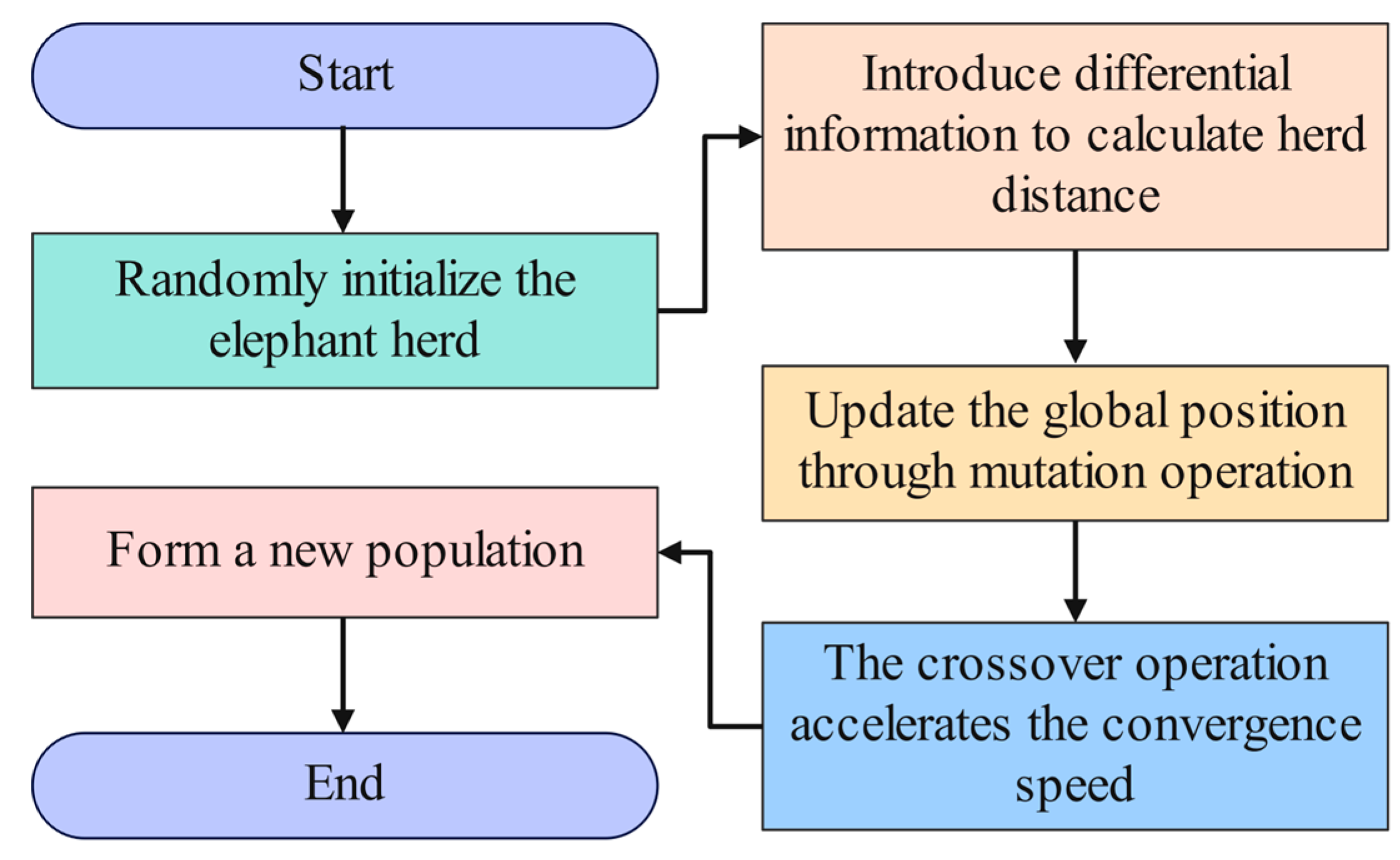
• In this research, by introducing differential information, we disrupt the originally relatively stable family structure and the leader selection process of the EHO algorithm. This disruption successfully promotes population variety. Apart from the Euclidean distance, differential information is added when determining the distance between people for family partition. The equation is displayed in Equation (18):

  $$d_{ij}=\sqrt{{\displaystyle \sum _{k=1}^n{(x_{ik}-x_{jk})}^2}}+\alpha \times |(x_{ik}-x_{jk})-(x_{i,k-1}-x_{j,k-1})|$$

  (18)

  here $\alpha$ is a regulatory parameter that regulates how much differential information is included in the distance computation. Equation (19) displays the formula for the thorough assessment value V of the leader selection:

  $$E_i=F(x_i)+\beta \times {\displaystyle \sum _{j=1,j\ne i}^N|x_{ij}-x_{jj}|}$$

  (19)

  in this case, $N$ is the population’s size, $\beta$ is the weight coefficient. The smaller the comprehensive evaluation value is, the more likely it is to become the leader.
• In this study, the individual update stage of the EHO algorithm introduces the mutation operation of the DE method. This enables individuals to conduct searches in a broader space, thus improving the algorithm’s capacity for worldwide search. Equation (20) displays the updated individual position update formula:

  $$x_{ij}^{t+1}=x_{ij}^t+r_1\times (x_{lj}^t-x_{ij}^t)+r_2\times (x_{gj}^t-x_{ij}^t)+F\times (x_a^t-x_b^t)$$

  (20)

  in this case, $x_a^t$ and $x_b^t$ represent the locations of two distinct people who were chosen at random from the population at the tth iteration. The Differential Evolution algorithm’s scaling factor, $F$, typically has a value between 0 and 2.
• Crossover operation of DE. For the individuals in EHO, the crossover operation is carried out with a certain crossover probability CR (usually between 0 and 1). Let $u_{ij}^{t+1}$ is the trial individual, and the improved crossover operation formula is shown in Equation (21):

  $$u_{ij}^{t+1}=\left\{\begin{array}{l}{v}_{ij}^{t+1},(rand(j)\le CR)\cup j=j_{rand}\\ x_{ij}^t,otherwise\end{array}\right.$$

  (21)

  in this case, $rand(j)$ is a randomly assigned number that ranges from 0 to 1. $j_{rand}$ is a randomly chosen dimension between 1 to D, where D is the problem’s dimension. $v_{ij}^{t+1}$ is the individual velocity attained following the above-described enhancement in the global search capability. Figure 5 introduces the flowchart of DE optimizing EHO.

2.6.6. CM Optimizes the Position Update of EHO

The Cauchy Mutation (CM) algorithm [62] uses the Cauchy distribution to carry out mutation operations on population members. It seeks to apply a more effective individual position update strategy and enhance the optimization method’s local search ability. The particular algorithm employed in this investigation is displayed as follows:

• During local search, the EHO algorithm is able to stay out of local optima. This is accomplished by utilizing the Cauchy distribution’s heavy-tailed characteristic. Equation (22) displays the Cauchy distribution’s density function for probability:

  $$f(x;x_0,\gamma )={\displaystyle \frac{1}{\pi \gamma [1+{(\frac{x-x_0}{\gamma })}^2]}}$$

  (22)

  the current individual position $x_i$ is typically used as the location parameter $x_0$ in local search, while the scale parameter $\gamma$ is selected according to the algorithm’s requirements and the problem’s nature.
• Through the integration of the Cauchy mutation, individuals are empowered to perform a more elaborate search in the neighborhood of their current locations. Equation (23) displays the updated formula:

  $$x_{ij}^{t+1}=x_{ij}^t+r_1\times (x_{lj}^t-x_{ij}^t)+r_2\times (x_{gj}^t-x_{ij}^t)+\delta \times Cauchy(0,1)$$

  (23)

  in this case, the parameter $\delta$ regulates the degree of Cauchy mutation. In this investigation, $Cauchy(0,1)$ represents a random number with a Cauchy distribution, a scale parameter of 1, and a location parameter of 0.
• Conduct local and global searches in a balanced manner. It is feasible to flexibly balance local and global search by dynamically modifying the settings of Cauchy mutation. Equation (24) illustrates the function of the Cauchy mutation intensity.

  $$\delta (t)={\delta }_0\times {(1-{\displaystyle \frac{t}{T}})}^{\lambda }$$

  (24)

  among them, ${\delta }_0$ is the initial Cauchy mutation intensity, $t$ represents the quantity of iterations underway, $T$ symbolizes the most iterations possible, and $\lambda$ is the parameter used to adjust the rate of change. The EHO flowchart optimized using CM is shown in Figure 6. EHO’s update approach and local search capability have greatly improved.

2.6.7. SPAD Value Inversion Model Based on CDE-EHO-GBM

By integrating the strengths of the DE algorithm in global search and convergence rate with the advantages of the CM in local optimization and position update, the operational efficiency and search performance of the EHO algorithm can be significantly enhanced. It is possible to raise the likelihood of discovering the worldwide ideal answer. The process diagram for enhancing the EHO algorithm by fusing DE and CM is displayed in Figure 7.

The specific steps of the canopy SPAD value inversion model of CDE-EHO-GBM are as follows:

(1)

Input the measured canopy SPAD values and the remote sensing image data from the UAV.

(2)

Feature selection. Raw vegetation indices were selected using CARS, FFS, and AFFS algorithms, and the screened key variables were input into the inversion models.

(3)

Create an inversion model for SPAD values depending on the GBM model.

(4)

Initialize the parameters. The number of iterations and the size of the elephant population were both determined to be 100, and the parameter ranges for this study are shown in

Table 3. GBM, RF, and PLSR model parameters and their significances.

Models	Parameters	Meaning	Range of Parameters
GBM	n_estimators	Number of iterations	50–300
	learning_rate	Learning rate	0.01–0.5
	max_depth	Maximum depth	3–10
	min_samples_split	The minimum number of samples at internal nodes	2–10
	min_samples_leaf	The minimum number of samples in leaf nodes	2–5
	subsample	The sample proportion of weak learners	0.5–1
	random_state	Random generator seed	30
RF	n_estimators	Number of iterations	50–300
	max_depth	Maximum depth	3–10
	min_samples_split	The minimum number of samples at internal nodes	2–10
PLSR	n_components	The number of latent variables	2–8
	max_iter	Maximum number of iterations	50–300
	tol	Iteration convergence threshold	0.00001–0.001
	scale	Boolean parameter	True

.

(5)

Define the fitness function. The fitness function used in this model is the Mean Squared Error (MSE). The higher the fitness, the lower the fitness function value. As Equation (25) illustrates:

$$Fitness=MSE={\displaystyle \frac{1}{n}}{\displaystyle \sum _{i=1}^n{(y_i-{\widehat{y}}_i)}^2}$$

(25)

here $y_i$ symbolizes the value that was really measured, and ${\widehat{y}}_i$ symbolizes the model’s anticipated value.

(6)

Determine the distance. Incorporate the differential information and calculate the distances between individual members of the elephant herd (according to Equation (18)).

(7)

Update the global position. Use crossover and mutation procedures to quicken the elephant herd’s rate of convergence (according to Equations (20) and (21)).

(8)

Conduct local optimization. Dynamically adjust the parameters of Cauchy mutation to shorten the search step size and examine the space of local optimal solutions (according to Equations (23) and (24)).

(9)

Update the best elephant herd’s location and fitness. Determine if the ceasing requirement is fulfilled. Continue to Step (10) if the requirement is met; if not, continue to Step (6).

(10)

Provide the precise position of the top herd of elephants (i.e., the optimal parameters of the CDE-EHO-GBM model).

(11)

Use the ideal parameters derived from the CDE-EHO technique to train the GBM model’s SPAD value inversion model and output the prediction SPAD results. Comparison of each model with measured SPAD data combined with calculation of evaluation metrics.

2.7. Model Evaluation Metrics

In this research, the coefficient of determination R², root-mean-square error (RMSE), and mean absolute error (MAE) served as the assessment metrics of the models. The model’s ability to describe the data improves as the R² score gets closer to 1. RMSE is sensitive to outliers, and a smaller value is better. MAE is not sensitive to outliers, resulting in more stable outcomes, and a smaller value is also better. The calculation formulas for R², RMSE, and MAE are shown in Equations (26), (27), and (28), respectively:

$$R^2=1-{\displaystyle \frac{{\displaystyle \sum _{i=1}^n{(y_i-{\widehat{y}}_i)}^2}}{{\displaystyle \sum _{i=1}^n{(y_i-\overline{y})}^2}}}$$

(26)

$$RMSE=\sqrt{{\displaystyle \frac{1}{n}}{\displaystyle \sum _{i=1}^n{(y_i-{\widehat{y}}_i)}^2}}$$

(27)

$$MAE={\displaystyle \frac{1}{n}}{\displaystyle \sum _{i=1}^n|y_i-{\widehat{y}}_i|}$$

(28)

here $y_i$ symbolizes the value that was really measured, ${\widehat{y}}_i$ indicates the model’s anticipated value, $\overline{y}$ symbolizes the average of the real values, and $n$ symbolizes the sample size.

3. Results and Analysis

3.1. Characteristic Statistics for Potato Canopy SPAD Values and Model Parameter Settings

The statistical study of potato canopy SPAD values at the seedling, tuber expansion, and cross-growth stages is shown in

Table 4. Statistical analysis of potato canopy SPAD values.

Fertility	Samples	Min	Max	Mean	Extreme Difference	Standard Deviation	Coefficient of Variation
Seedling stage	162	40.30	56.00	48.47	15.70	3.70	7.63%
Tuber expansion stage	162	28.20	54.20	43.20	26.00	5.40	12.50%
Cross-growth stage	324	28.20	56.00	45.84	27.80	5.33	11.63%

.

Model parameters significantly affect efficiency and accuracy. Table 3 presents the parameter ranges and their corresponding definitions for the Gradient Boosting Machine (GBM), Random Forest (RF), and Partial Least Squares Regression (PLSR) models employed within this study.

3.2. The Selection Results of VIs

The CARS algorithm is founded on adaptive re-weighting and Monte Carlo sampling techniques. It eliminates variable subsets that significantly affect the model through multiple sampling operations and variable weight updates. After several iterations, it selects a subset of variables with the strongest explanatory power for potato canopy SPAD values from numerous VIs and inputs them into the GBM model. Figure 8 shows the VI feature selection procedure of the GBM model at the potato seedling stage. The RMSECV varies constantly as the iteration goes on, and the number of chosen VIs exhibits a declining trend. At the end of the iteration, it can be seen that the number of iterations reaches 10 and the RMSECV reaches its lowest value. At this point the corresponding 10 VIs were identified as input variables for the GBM model, namely MCARI, MTVI, EVI2, RECI, GCI, NDVI, RVI, MSRI, OSAVI, and GRRI. Figure 8 displays their distribution characteristics.

The FFS algorithm implements a greedy approach. It initiates with an empty feature subset. In each iteration, it adds a feature to the current subset, provided that specific stopping criteria are not yet met. The optimal VI subsets selected by the FFS method are shown in

Table 5. Results of variable selection.

Feature Extraction	Seedling Stage									Tuber Expansion Stage									Cross-Growth Stage
	CARS			FFS			AFFS			CARS			FFS			AFFS			CARS			FFS			AFFS
	GBM	RF	PLSR	GBM	RF	PLSR	GBM	RF	PLSR	GBM	RF	PLSR	GBM	RF	PLSR	GBM	RF	PLSR	GBM	RF	PLSR	GBM	RF	PLSR	GBM	RF	PLSR
GRVI												√		√			√
MCARI	√										√			√	√		√							√
DVI								√			√		√	√	√		√	√	√			√			√	√
MTVI	√							√			√													√
WDRVI					√		√										√		√	√	√	√	√	√	√	√	√
EVI2	√	√		√	√		√	√	√								√			√						√
RECI	√								√	√					√									√
GCI	√			√					√	√	√		√		√	√	√	√		√		√				√
NDVI	√	√	√	√	√	√	√	√	√								√	√						√		√
GNDVI		√		√	√			√											√	√		√	√			√	√
RVI	√	√	√	√	√	√	√	√	√					√			√							√
NDGI		√												√			√							√		√
MSRI	√	√	√	√	√	√	√	√	√												√			√
OSAVI	√	√	√	√	√	√	√	√	√																	√	√
SRI							√						√		√	√
NDRE											√						√							√
NLI		√		√	√		√				√	√		√	√				√					√		√
TVI											√							√	√	√	√					√
GRRI	√						√				√					√				√		√
RNVI		√		√							√							√

. Nine VIs, including EVI2, were chosen by the GBM model during the seedling stage, eight by the RF model, including WDRVI, and four by the PLSR model, including NDVI. Three VIs, like DVI, were chosen by the GBM model, six VIs, like GRVI, by the RF model, and six VIs, like MCARI, by the PLSR model during the tuber expansion stage. The GBM model chose five VIs, like DVI, the RF model chose two, like WDRVI, and the PLSR model chose ten, like MCARI, during the cross-growth stage. The FFS algorithm inputs the above-selected features into the learning models by progressively selecting the VIs that are most beneficial for objective function optimization. This provides the model with relatively streamlined and effective input features, which improves the performance of the GBM, RF, and PLSR models to some extent, but is slightly less effective than the AFFS algorithm.

The AFFS algorithm incorporates an adaptive mechanism. It dynamically modifies the feature selection method to more flexibly and effectively choose the most representative and discriminative VI. Table 5 presents the findings. The GBM model chose nine VIs, including WDRVI, the RF model chose eight, including DVI, and the PLSR model chose seven, including EVI2, during the seedling stage. The RF model selected ten Vis, like GRVI, the PLSR model selected five Vis, like DVI, and the GBM model selected three Vis, like GCI, during the tuber expansion stage. The GBM model selected two VIs, such as DVI, the RF model selected ten VIs, such as DVI, and the PLSR model selected three VIs, such as WDRVI, at the cross-growth stage. In addition to choosing feature bands more precisely, the AFFS algorithm can also steer clear of information redundancy and unnecessary computations. The AFFS algorithm dynamically adjusts the weights of VIs, and if certain VIs are found to cause overfitting, their weights will be reduced or directly eliminated. The VIs selected above are input into each model to reduce information redundancy and unnecessary calculations, and significantly improve the performance of GBM, RF, and PLSR models. Table 5 lists the VI selection variables used in this investigation.

3.3. Analysis of Model Performance Based on VIs

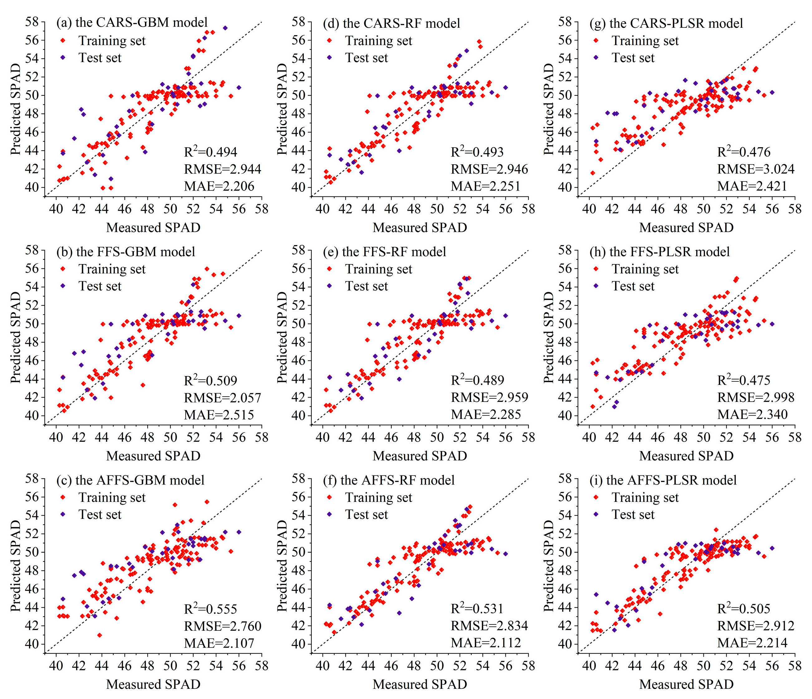
3.3.1. Analysis of Selection Algorithms and Model Performance During the Seedling Stage

In this research, we applied the GBM, RF, and PLSR models to carry out an inversion analysis of the potato canopy SPAD values.

Table 6. Results of various feature extraction methods’ model inversion during the potato seedling stage.

Models	Feature Extraction	Train Data			Test Data
		R2	RMSE	MAE	R2	RMSE	MAE
GBM	CARS	0.713	1.914	1.488	0.494	2.944	2.206
	FFS	0.708	1.928	1.479	0.509	2.057	2.515
	AFFS	0.754	1.770	1.396	0.555	2.760	2.107
RF	CARS	0.710	1.921	1.478	0.493	2.946	2.251
	FFS	0.709	1.827	1.387	0.489	2.959	2.285
	AFFS	0.770	1.713	1.316	0.531	2.834	2.112
PLSR	CARS	0.625	2.187	1.653	0.476	3.024	2.421
	FFS	0.683	2.010	1.566	0.475	2.998	2.340
	AFFS	0.770	1.712	1.322	0.505	2.912	2.214

The optimal model is indicated in bold.

exhibits the inversion results of several feature extraction algorithms during the potato seedling stage.

Experimental results indicate that the GBM, RF, and PLSR models all have R² values greater than 0.500. The AFFS-GBM model exhibited the best performance, and the R², RMSE, and MAE were 0.555, 2.760, and 2.107. In this section, the accuracy has been greatly increased without the use of optimization algorithms, in contrast to our team’s earlier research, where the R² value was less than 0.500 [63]. Consequently, the employment of feature selection by the AFFS algorithm in future inversion experiments of this study is expected to lead to a remarkable enhancement in research accuracy. The scatter plots of the observed canopy SPAD values and those determined by various models using various feature selection methods at the potato seedling stage are shown in Figure 9.

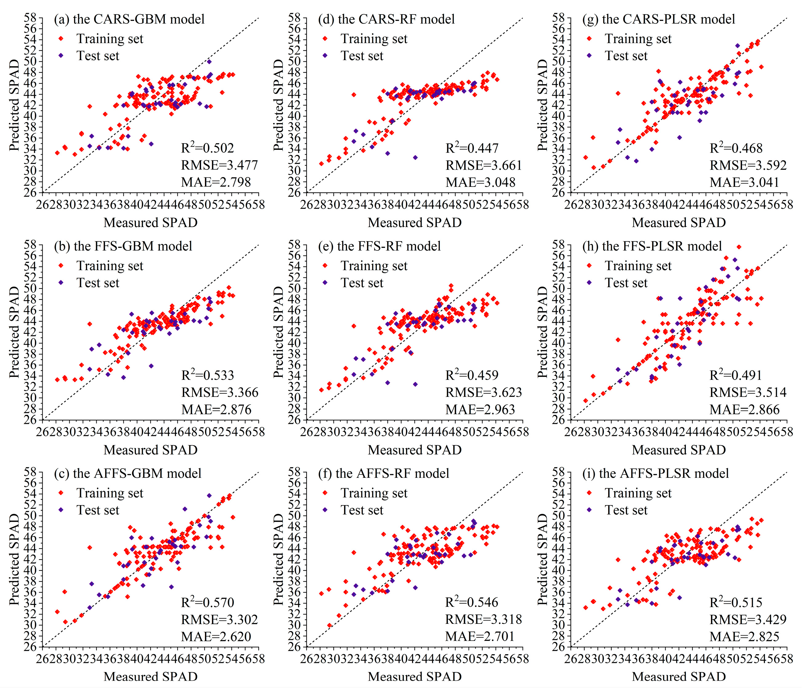
3.3.2. Analysis of Selection Algorithms and Model Performance During the Tuber Expansion Stage

During the tuber expansion stage of potatoes, various feature selection algorithms were combined with three models to carry out an inversion study on the canopy SPAD values, yielding diverse outcomes.

Table 7. Model inversion outcomes of various algorithms for feature extraction during the potato tuber expansion stage.

Models	Feature Extraction	Train Data			Test Data
		R2	RMSE	MAE	R2	RMSE	MAE
GBM	CARS	0.545	3.713	3.197	0.502	3.477	2.798
	FFS	0.745	2.780	2.211	0.533	3.366	2.876
	AFFS	0.715	2.937	2.009	0.570	3.302	2.620
RF	CARS	0.607	3.451	2.748	0.447	3.661	3.048
	FFS	0.657	3.223	2.565	0.459	3.623	2.963
	AFFS	0.514	3.838	3.232	0.546	3.318	2.701
PLSR	CARS	0.753	2.737	1.768	0.468	3.592	3.041
	FFS	0.652	3.246	2.394	0.491	3.514	2.866
	AFFS	0.556	3.669	3.156	0.515	3.429	2.825

The optimal model is indicated in bold.

displays the outcomes of the inversion.

Experimental results demonstrate that the incorporation of the adaptive mechanism enhanced the inversion accuracy of the AFFS algorithm. For both training and testing sets, the AFFS-GBM model performs at its best. R² values for the training and test sets were 0.715 and 0.570, while their corresponding RMSE values were 2.937 and 3.302. The greatest R² value in our team’s earlier research, without optimization techniques, was 0.51. As a result, this study’s accuracy is much higher than earlier research, and the RMSE has also greatly dropped. Figure 10 displays the scatter plot of each model’s actual and anticipated values.

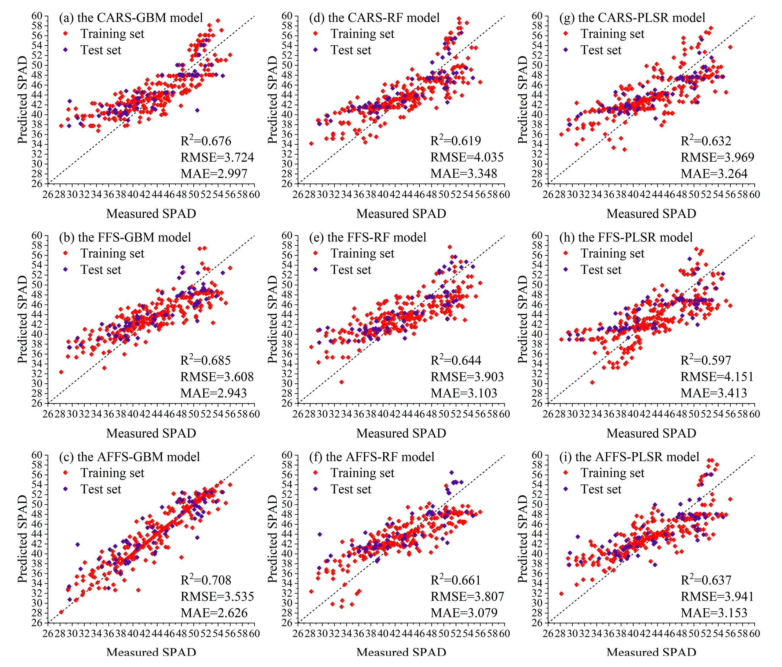
3.3.3. Analysis of Selection Algorithms and Model Performance During the Cross-Growth Stage

During the cross-growth stage, the VIs selected by the CARS, FFS, and AFFS algorithms were employed as inputs for the three models to conduct an inversion investigation of canopy SPAD values. The outcomes of the inversion are presented in

Table 8. Results of model inversion using various feature extraction techniques during the cross-growth stage of potatoes.

Models	Feature Extraction	Train Data			Test Data
		R2	RMSE	MAE	R2	RMSE	MAE
GBM	CARS	0.718	3.299	2.589	0.676	3.724	2.997
	FFS	0.766	3.002	2.310	0.685	3.608	2.943
	AFFS	0.851	2.394	1.462	0.708	3.535	2.626
RF	CARS	0.669	3.570	2.834	0.619	4.035	3.348
	FFS	0.681	3.507	2.752	0.644	3.903	3.103
	AFFS	0.777	2.929	2.338	0.661	3.807	3.079
PLSR	CARS	0.680	3.511	2.772	0.632	3.969	3.264
	FFS	0.609	3.886	3.058	0.597	4.151	3.413
	AFFS	0.733	3.207	2.509	0.637	3.941	3.153

The optimal model is indicated in bold.

.

Based on the experimental results, the AFFS-GBM model exhibits superior performance compared to the other models in both the test set and the training set. For the training and test sets, R² values were 0.851 and 0.708, RMSE values were 2.394 and 3.535, and MAE values were 1.462 and 2.626. Within the AFFS-RF and AFFS-PLSR models, 0.661 and 0.637 were the matching R² values for the prediction sets, and their respective RMSE values were 3.807 and 3.941. The accuracy has somewhat improved when compared to earlier research. Figure 11 displays the scatter plot of each model’s actual and anticipated values at the potato cross-growth stage.

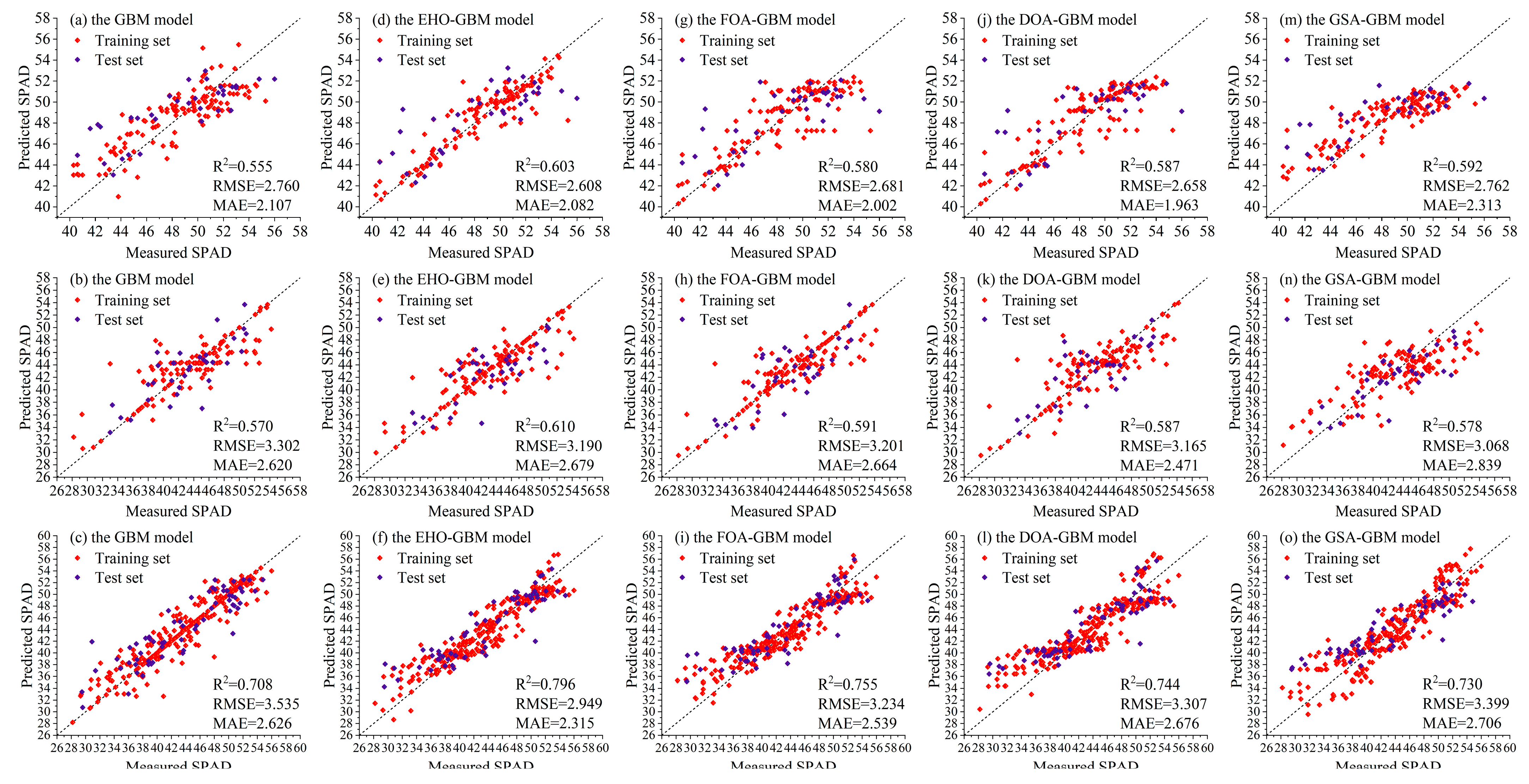
3.4. Intelligent Algorithms for Optimizing the GBM Model

The central aim of this research is to carry out an inversion study on potato canopy SPAD values employing the AFFS-GBM model. As presented in Table 3, the GBM model incorporates a series of parameters. Intelligent optimization algorithms are able to identify the best parameter configurations and enhance the model’s overall performance. This study improved the GBM model’s precision using EHO, FOA, DOA, and GSA. The GBM model’s optimization findings are shown in

Table 9. Optimization results of the GBM model by various optimization algorithms in different growth stages.

Growth Stage	Optimization Algorithm	Train Data			Test Data
		R2	RMSE	MAE	R2	RMSE	MAE
Seedling stage	GBM	0.754	1.770	1.396	0.555	2.760	2.107
	EHO-GBM	0.829	1.475	1.014	0.603	2.608	2.082
	FOA-GBM	0.722	1.881	1.365	0.580	2.681	2.002
	DOA-GBM	0.700	1.954	1.522	0.587	2.658	1.963
	GSA-GBM	0.690	1.986	1.605	0.592	2.762	2.313
Tuber expansion stage	GBM	0.715	2.937	2.009	0.570	3.302	2.620
	EHO-GBM	0.757	2.712	1.776	0.610	3.190	2.679
	FOA-GBM	0.777	2.929	2.338	0.591	3.201	2.664
	DOA-GBM	0.710	2.965	2.055	0.587	3.165	2.471
	GSA-GBM	0.663	3.616	2.116	0.578	3.068	2.839
Cross-growth stage	GBM	0.851	2.394	1.462	0.708	3.535	2.626
	EHO-GBM	0.866	2.273	1.715	0.796	2.949	2.315
	FOA-GBM	0.841	2.477	1.919	0.755	3.234	2.539
	DOA-GBM	0.772	2.966	2.329	0.744	3.307	2.676
	GSA-GBM	0.756	3.158	2.386	0.730	3.399	2.706

The optimal model is indicated in bold.

.

It is easily seen that the GBM model’s accuracy has increased across all of the development stages because of the optimization procedures. The EHO-GBM model exhibits the best optimization result at the cross-growth stage. The R² values were 0.866 and 0.796, the RMSE values were 2.273 and 2.949, and the MAE values were 1.715 and 2.315. The traditional GSA algorithm yields lower results than the AFFS algorithm, mainly because it only searches within a predetermined range of parameters and can easily fall into local optimal solutions. The outcomes of the GBM model’s parameter optimization using various optimization strategies for each period are displayed in Figure 12. To improve the precision of the study’s conclusions, an inversion investigation of canopy SPAD values is carried out in this study using the EHO method in conjunction with the GBM model.

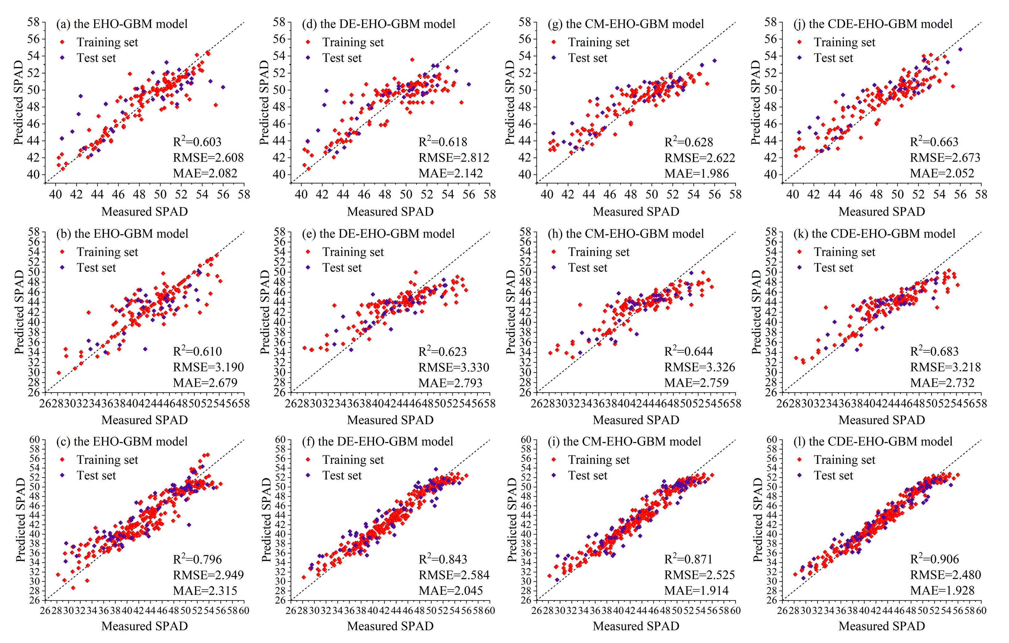
3.5. The CDE-EHO-GBM Model Based on the Improved Algorithms

In this study, integrating DE and CM enhanced the EHO algorithm, which significantly enhanced the precision of the outcomes and the model’s operating efficiency.

Table 10. Results of improving the EHO-GBM model by different algorithms.

Growth Stage	Optimization Algorithm	Train Data			Test Data
		R2	RMSE	MAE	R2	RMSE	MAE
Seedling stage	EHO-GBM	0.829	1.475	1.014	0.603	2.608	2.082
	DE-EHO-GBM	0.789	1.325	1.217	0.618	2.812	2.142
	CM-EHO-GBM	0.772	1.705	1.361	0.628	2.622	1.986
	CDE-EHO-GBM	0.777	1.686	1.350	0.663	2.673	2.052
Tuber expansion stage	EHO-GBM	0.757	2.712	1.776	0.610	3.190	2.679
	DE-EHO-GBM	0.654	3.240	2.550	0.623	3.330	2.793
	CM-EHO-GBM	0.707	2.982	2.316	0.644	3.326	2.759
	CDE-EHO-GBM	0.771	2.634	1.953	0.683	3.218	2.732
Cross-growth stage	EHO-GBM	0.866	2.273	1.715	0.796	2.949	2.315
	DE-EHO-GBM	0.959	1.243	0.936	0.843	2.584	2.045
	CM-EHO-GBM	0.954	1.189	0.928	0.871	2.525	1.914
	CDE-EHO-GBM	0.964	1.170	0.889	0.906	2.480	1.928

The optimal model is indicated in bold.

shows that the accuracy of the GBM model enhanced by diverse techniques has experienced a substantial increase over the span of multiple growth stages. Interestingly, the CDE-EHO-GBM model continuously shows the highest accuracy, suggesting that the method that combines DE and CM improves EHO the most.

The CDE-EHO-GBM model outperforms other improved models on both the test and training sets. Especially during the cross-growth stage, the precision reached its highest level. The R² values were 0.964 and 0.906, the RMSE values were 1.170 and 2.480, and the MAE values were 0.889 and 1.928, respectively. The greatest R² value in our team’s earlier research was 0.600 during the seedling stage, 0.660 during the tuber expansion stage, and 0.870 during the cross-growth stage. In each growth stage, the optimal results of this study are significantly superior to those of previous research. Considering the great difficulty in enhancing the accuracy of scientific research, the findings of this study represent remarkable progress in comparison with prior investigations. The CDE-EHO-GBM model predicts canopy SPAD values with the highest accuracy, as seen in Figure 13, and is closest to the measured values.

Table 11. Optimal parameter results of the optimal model for each stage.

Models	Parameters	Seedling Stage AFFS-GBM	Tuber Expansion Stage AFFS-GBM	Cross-Growth Stage AFFS-GBM	Cross- Growth Stage EHO-GBM	Cross- Growth Stage CDE-EHO-GBM
GBM	n_estimators	133	97	253	145	175
	learning_rate	0.50	0.32	0.15	0.22	0.35
	max_depth	7	6	8	6	9
	min_samples_split	5	7	4	5	3
	min_samples_leaf	2	4	4	5	3
	subsample	0.52	0.61	0.82	0.65	0.74
	random_state	30	30	30	30	30

shows the results of the optimal parameters of the optimal model for each stage in this study.

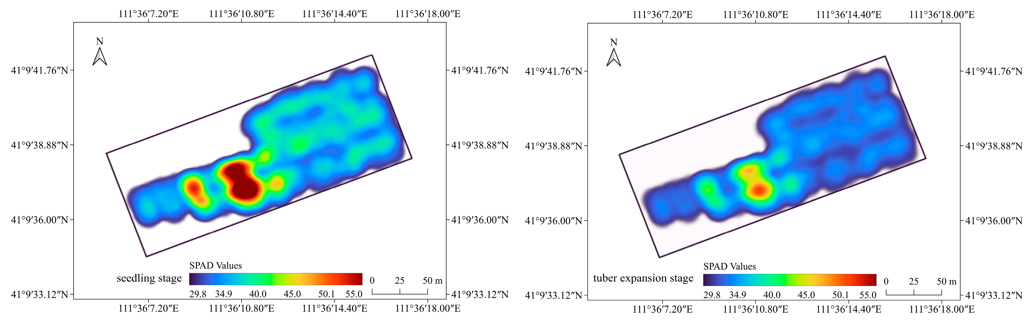
3.6. Temporal and Spatial Distribution of Chlorophyll Content in Potato Canopy

As can be seen from the above experiments, the CDE-EHO-GBM model proposed in this paper exhibits the best performance. We drew the temporal–spatial distribution map of canopy chlorophyll content based on the inversion results of this model, as shown in Figure 14. The canopy chlorophyll content is generally high during the seedling stage and relatively low during the tuber expansion stage. This is mainly because during the seedling stage, potato plants are in the vegetative growth phase. To meet the demand for intense photosynthesis, the chlorophyll content accumulates and increases rapidly at this time. When entering the tuber expansion stage, the focus of the plant’s physiological activities shifts to tuber maturation and nutrient accumulation. The leaves gradually senesce, the degradation of chlorophyll accelerates, and its content decreases.

The varieties with the darkest color and the highest chlorophyll content in the figure are Favorita and Xufeng No.1. This is due to the strong growth vigor of the potato plants of these two varieties. During growth, plants with high growth vigor rapidly synthesize more chlorophyll and improve photosynthetic efficiency [64]. In the same growth stage, the chlorophyll content of potatoes in different plots may also vary. This may be due to the unevenness of factors such as soil fertility, irrigation conditions, and light intensity between different plots. Within the same plot, some early-maturing varieties may complete their growth cycle in a shorter time, and their chlorophyll content changes relatively quickly. In contrast, late-maturing varieties may have a longer growth cycle, and their chlorophyll content changes more slowly. At the same time, combining chlorophyll content data from multiple scales, such as leaves, canopy, plots, and regions, for comprehensive analysis and modeling can become a direction for future research. In order to conduct a comparative analysis of the temporal and spatial distribution maps of the two periods, the legends set in Figure 14 are consistent.

4. Discussion

In this study, the AFFS algorithm was used to improve the effect of feature selection, and a CDE-EHO-GBM model was developed to conduct an inversion study on the chlorophyll content of the potato canopy. A variety of feature-extraction techniques, ML models, and parameter-optimization strategies can exert a substantial influence on the inversion results. The following is a discussion of the experimental results.

Different VIs may contain some overlapping information, leading to a certain degree of information redundancy. Eliminating unnecessary VIs through feature selection is very important. As a result, the model can concentrate on the most discriminative and representative features, improving its capacity for generalization, avoiding overfitting, and lessening its computational load [65]. The findings indicate that the inversion outcomes of the AFFS algorithm are more precise. The results during the cross-growth stage are the best. The values of R² reached 0.851 and 0.708, while the values of RMSE were 2.394 and 3.535. When working with data that has intricate and extremely non-linear interaction relationships, the CARS algorithm is unstable. It could produce less-than-ideal feature selection outcomes since it is unable to adequately represent the intricate relationships present in the data [66]. To avoid being trapped in local optimal solutions, an adaptive mechanism is employed to dynamically adjust the feature—selection strategy and adaptively alter the search direction in accordance with the feedback information obtained during the search process. As a result, the AFFS algorithm is capable of yielding the optimal inversion results. If VIs are not selected, the unselected VIs contain a large amount of repetitive and redundant information, which not only increases the computational burden of the model but also interferes with the model’s ability to capture critical information. The AFFS algorithm selects the most representative and discriminative VIs by dynamically modifying the weights of the VIs, which can provide more direct and effective information for the model and reduce the error of the model.

In this research, the EHO, FOA, DOA, and GSA algorithms were subsequently introduced to enhance the GBM model’s precision. According to the findings, during every growth stage, the EHO algorithm has the best optimization effect. During the seedling stage, tuber expansion stage, and cross-growth stage, the R² values of the test set are 0.603, 0.610, and 0.796, respectively. The EHO algorithm deeply simulates the complex social structure and behavioral patterns of elephant herds, aiming to solve the optimization problems of biological populations in a more comprehensive and detailed manner [67]. On the contrary, the FOA and DOA algorithms simulate biological characteristics in a relatively simplistic way. When dealing with complex problems, they may lack the adaptability demonstrated by the EHO algorithm, which is based on a diverse set of behavioral patterns and a profound social structure. The GSA algorithm relies on pre-set parameter ranges and step sizes. As a result, the model is prone to falling into local optimization and lacks the ability to make dynamic adjustments.

We incorporated the DE and CM algorithms to enhance the EHO optimization algorithm in the study, and we significantly augmented the parameter-optimization capability of the enhanced EHO algorithm. According to the inversion results, the most accurate model is the CDE-EHO-GBM model. On the test sets of the seedling stage, tuber expansion stage, and cross-growth stage, the R² values are 0.663, 0.683, and 0.906, the RMSE values are 2.673, 3.218, and 2.480, respectively. DE allows for the investigation of new solution spaces across a wide range by primarily directing the search direction through the differential vectors across population individuals. It might, however, occasionally become stuck in local optima [68]. Near the ideal solution, CM can carry out a more thorough search. Nevertheless, its ability and convergence efficiency are quite low when it is far from the perfect solution [69]. The combination of the two enables the improved EHO algorithm not only to rapidly approach the optimal solution during the convergence process but also to more precisely find the optimal solution’s location, thereby improving the model’s efficiency. This study significantly improved the accuracy in terms of R², RMSE, and MAE compared to our team’s earlier research, suggesting that substantial progress has been made on the original premise. However, there remain areas for improvement in the enhanced algorithms of this study. For instance, the model exhibits relatively low stability, and the algorithm execution time is rather long. To reduce memory consumption and the sensitivity to initial parameters, future research could explore parallel computing platforms or alternative algorithms.

This study examined the trends and variations of SPAD values and data models at various development stages by combining two crucial growth periods in the potato growth process. Furthermore, in this experiment, the cross-growth period had a higher inversion accuracy than the seedling and tuber expansion stages. This suggests that it is crucial to investigate and test SPAD values and remote sensing data from many growth periods in addition to data from a single growth period. This method can save a significant amount of time, money, and human resources by more correctly estimating the general trend of the potato growth cycle. It is extremely important for the large-scale field assessment of potato SPAD values. At the same time, ML algorithms can analyze multispectral and hyperspectral images captured by UAVs or satellites to detect early signs of diseases like late blight, early blight, and potato Y virus. Also, ML models can integrate various data sources, such as weather data, soil properties, and historical yield records, to accurately predict potato yields. These issues and applications are crucial for potato planting, harvesting, and marketing management, and can be further studied in the future.

5. Conclusions

In this study, the AFFS technique is integrated with the CDE-EHO-GBM model to address the pressing issue of estimating potato canopy SPAD values across diverse growth phases. By adding an adaptive mechanism to the FFS approach, the GBM model’s complexity can be decreased and the inversion precision increased. Based on the AFFS algorithm, a CDE-EHO-GBM model integrating the DE algorithm and the CM algorithm was developed, which has led to a significant enhancement in accuracy during various growth periods. The training and test sets’ respective R² values were 0.964 and 0.906, indicating a substantial rise in accuracy over previous studies, especially during the cross-growth period.

Despite the remarkable achievements of this study in vegetation feature selection and the accuracy of model optimization, several limitations persist. In particular, UAV resolution and weather conditions during data collection limited the training data. In future research, it is proposed to investigate alternative data and algorithms in an effort to increase the precision of canopy SPAD value estimation. It is possible to introduce deep learning models to better handle complex nonlinear relationships and spatiotemporal dependencies. We can also analyze and model the chlorophyll content of potatoes at multiple scales (such as leaf, canopy, plot, and regional scales) to better understand the physiological and ecological processes and environmental impact factors at different scales. This approach promises to significantly advance precision fertilization strategies and improve yield prediction accuracy in potato cultivation.

References

1. Wang, Z.-J.; Liu, H.; Zeng, F.-K.; Yang, Y.-C.; Xu, D.; Zhao, Y.-C.; Liu, X.-F.; Kaur, L.; Liu, G.; Singh, J. Potato Processing Industry in China: Current Scenario, Future Trends and Global Impact. Potato Res. 2023, 66, 543–562. [Google Scholar] [CrossRef]
2. Ma, Y.; Qiu, C.; Zhang, J.; Pan, D.; Zheng, C.; Sun, H.; Feng, H.; Song, X. Potato Leaf Chlorophyll Content Estimation through Radiative Transfer Modeling and Active Learning. Agronomy 2023, 13, 3071. [Google Scholar] [CrossRef]
3. Shi, H.; Lu, X.; Sun, T.; Liu, X.; Huang, X.; Tang, Z.; Li, Z.; Xiang, Y.; Zhang, F.; Zhen, J. Monitoring of Chlorophyll Content of Potato in Northern Shaanxi Based on Different Spectral Parameters. Plants 2024, 13, 1314. [Google Scholar] [CrossRef]
4. Mandal, B.K.; Ling, Y.-C. Analysis of Chlorophylls/Chlorophyllins in Food Products Using HPLC and HPLC-MS Methods. Molecules 2023, 28, 4012. [Google Scholar] [CrossRef]
5. Mohsan, S.A.H.; Othman, N.Q.H.; Li, Y.; Alsharif, M.H.; Khan, M.A. Unmanned aerial vehicles (UAVs): Practical aspects, applications, open challenges, security issues, and future trends. Intell. Serv. Robot. 2023, 16, 109–137. [Google Scholar] [CrossRef]
6. Yang, H.; Hu, Y.; Zheng, Z.; Qiao, Y.; Hou, B.; Chen, J. A New Approach for Nitrogen Status Monitoring in Potato Plants by Combining RGB Images and SPAD Measurements. Remote Sens. 2022, 14, 4814. [Google Scholar] [CrossRef]
7. Ma, W.; Han, W.; Zhang, H.; Cui, X.; Zhai, X.; Zhang, L.; Shao, G.; Niu, Y.; Huang, S. UAV multispectral remote sensing for the estimation of SPAD values at various growth stages of maize under different irrigation levels. Comput. Electron. Agric. 2024, 227, 109566. [Google Scholar] [CrossRef]
8. Yang, H.; Hu, Y.; Zheng, Z.; Qiao, Y.; Zhang, K.; Guo, T.; Chen, J. Estimation of Potato Chlorophyll Content from UAV Multispectral Images with Stacking Ensemble Algorithm. Agronomy 2022, 12, 2318. [Google Scholar] [CrossRef]
9. Awad, M.M. An innovative intelligent system based on remote sensing and mathematical models for improving crop yield estimation. Inf. Process. Agric. 2019, 6, 316–325. [Google Scholar] [CrossRef]
10. Tian, B.; Yu, H.; Zhang, S.; Wang, X.; Yang, L.; Li, J.; Cui, W.; Wang, Z.; Lu, L.; Lan, Y.; et al. Inversion of Cotton Soil and Plant Analytical Development Based on Unmanned Aerial Vehicle Multispectral Imagery and Mixed Pixel Decomposition. Agriculture 2024, 14, 1452. [Google Scholar] [CrossRef]
11. Elarab, M.; Ticlavilca, A.M.; Torres-Rua, A.F.; Maslova, I.; McKee, M. Estimating chlorophyll with thermal and broadband multispectral high resolution imagery from an unmanned aerial system using relevance vector machines for precision agriculture. Int. J. Appl. Earth Obs. Geoinf. 2015, 43, 32–42. [Google Scholar] [CrossRef]
12. Singhal, G.; Bansod, B.; Mathew, L.; Goswami, J.; Choudhury, B.U.; Raju, P.L.N. Chlorophyll estimation using multi-spectral unmanned aerial system based on machine learning techniques. Remote Sens. Appl. Soc. Environ. 2019, 15, 100235. [Google Scholar] [CrossRef]
13. Wu, Q.; Zhang, Y.; Zhao, Z.; Xie, M.; Hou, D. Estimation of Relative Chlorophyll Content in Spring Wheat Based on Multi-Temporal UAV Remote Sensing. Agronomy 2023, 13, 211. [Google Scholar] [CrossRef]
14. Sarvakar, K.; Thakkar, M. Different Vegetation Indices Measurement Using Computer Vision. In Applications of Computer Vision and Drone Technology in Agriculture 4.0; Chouhan, S.S., Singh, U.P., Jain, S., Eds.; Springer Nature: Singapore, 2024; pp. 133–163. [Google Scholar]
15. Xu, C.; Ding, Y.; Zheng, X.; Wang, Y.; Zhang, R.; Zhang, H.; Dai, Z.; Xie, Q. A Comprehensive Comparison of Machine Learning and Feature Selection Methods for Maize Biomass Estimation Using Sentinel-1 SAR, Sentinel-2 Vegetation Indices, and Biophysical Variables. Remote Sens. 2022, 14, 4083. [Google Scholar] [CrossRef]
16. Guo, X.; Wang, R.; Chen, J.M.; Cheng, Z.; Zeng, H.; Miao, G.; Huang, Z.; Guo, Z.; Cao, J.; Niu, J. Synergetic inversion of leaf area index and leaf chlorophyll content using multi-spectral remote sensing data. Geo-Spat. Inf. Sci. 2025, 28, 22–35. [Google Scholar] [CrossRef]
17. Houborg, R.; Soegaard, H.; Boegh, E. Combining vegetation index and model inversion methods for the extraction of key vegetation biophysical parameters using Terra and Aqua MODIS reflectance data. Remote Sens. Environ. 2007, 106, 39–58. [Google Scholar] [CrossRef]
18. Carmona, F.; Rivas, R.E.; Fonnegra, D. Vegetation Index to estimate chlorophyll content from multispectral remote sensing data. Eur. J. Remote Sens. 2015, 48, 319–326. [Google Scholar] [CrossRef]
19. Elbasi, E.; Zaki, C.; Topcu, A.E.; Abdelbaki, W.; Zreikat, A.I.; Cina, E.; Shdefat, A.; Saker, L. Crop Prediction Model Using Machine Learning Algorithms. Appl. Sci. 2023, 13, 9288. [Google Scholar] [CrossRef]
20. Mishra, H.; Mishra, D. Artificial Intelligence and Machine Learning in Agriculture: Transforming Farming Systems. In Research Trends in Agriculture Science; Bhumi Publishing: Kolhapur, India, 2023; pp. 1–16. [Google Scholar]
21. Kumari, S.; Venkatesh, V.G.; Tan, F.T.C.; Bharathi, S.V.; Ramasubramanian, M.; Shi, Y. Application of machine learning and artificial intelligence on agriculture supply chain: A comprehensive review and future research directions. Ann. Oper. Res. 2025, 348, 1573–1617. [Google Scholar] [CrossRef]
22. Wang, T.; Gao, M.; Cao, C.; You, J.; Zhang, X.; Shen, L. Winter wheat chlorophyll content retrieval based on machine learning using in situ hyperspectral data. Comput. Electron. Agric. 2022, 193, 106728. [Google Scholar] [CrossRef]
23. Shah, S.H.; Angel, Y.; Houborg, R.; Ali, S.; McCabe, M.F. A Random Forest Machine Learning Approach for the Retrieval of Leaf Chlorophyll Content in Wheat. Remote Sens. 2019, 11, 920. [Google Scholar] [CrossRef]
24. Pan, F.; Li, W.; Lan, Y.; Liu, X.; Miao, J.; Xiao, X.; Xu, H.; Lu, L.; Zhao, J. SPAD inversion of summer maize combined with multi-source remote sensing data. Int. J. Precis. Agric. Aviat. 2018, 1, 45–52. [Google Scholar] [CrossRef]
25. Zhao, X.; Qi, J.; Jiang, J.; Liu, S.; Xu, H.; Lin, S.; Yu, Z.; Li, L.; Huang, H. Fine-scale retrieval of leaf chlorophyll content using a semi-empirically accelerated 3D radiative transfer model. Int. J. Appl. Earth Obs. Geoinf. 2024, 135, 104285. [Google Scholar] [CrossRef]
26. Li, W.; Pan, K.; Liu, W.; Xiao, W.; Ni, S.; Shi, P.; Chen, X.; Li, T. Monitoring Maize Canopy Chlorophyll Content throughout the Growth Stages Based on UAV MS and RGB Feature Fusion. Agriculture 2024, 14, 1265. [Google Scholar] [CrossRef]
27. Elsayed, S.; El-Hendawy, S.; Elsherbiny, O.; Okasha, A.; El-Metwalli, A.; Elwakeel, A.; Memon, D.-M.S.; Ibrahim, M.; Ibrahim, H. Estimating Chlorophyll Content, Production, and Quality of Sugar Beet under Various Nitrogen Levels Using Machine Learning Models and Novel Spectral Indices. Agronomy 2023, 13, 104285. [Google Scholar] [CrossRef]
28. Aliferis, C.; Simon, G. Overfitting, Underfitting and General Model Overconfidence and Under-Performance Pitfalls and Best Practices in Machine Learning and AI. In Artificial Intelligence and Machine Learning in Health Care and Medical Sciences: Best Practices and Pitfalls; Simon, G.J., Aliferis, C., Eds.; Springer International Publishing: Cham, Germany, 2024; pp. 477–524. [Google Scholar]
29. Wang, J.; Lin, D.; Zhang, Y.; Huang, S. An adaptively balanced grey wolf optimization algorithm for feature selection on high-dimensional classification. Eng. Appl. Artif. Intell. 2022, 114, 105088. [Google Scholar] [CrossRef]
30. Alizamir, M.; Heddam, S.; Kim, S.; Mehr, A.D. On the implementation of a novel data-intelligence model based on extreme learning machine optimized by bat algorithm for estimating daily chlorophyll-a concentration: Case studies of river and lake in USA. J. Clean. Prod. 2021, 285, 124868. [Google Scholar] [CrossRef]
31. Lu, J.; Qiu, H.; Zhang, Q.; Lan, Y.; Wang, P.; Wu, Y.; Mo, J.; Chen, W.; Niu, H.; Wu, Z. Inversion of chlorophyll content under the stress of leaf mite for jujube based on model PSO-ELM method. Front. Plant Sci. 2022, 13, 1009630. [Google Scholar] [CrossRef]
32. Wu, C.; Fu, X.; Li, H.; Hu, H.; Li, X.; Zhang, L. A Method Based on Improved Ant Colony Algorithm Feature Selection Combined With GA-SVR Model for Predicting Chlorophyll-a Concentration in Ulansuhai Lake. IEEE Access 2023, 11, 93180–93192. [Google Scholar] [CrossRef]
33. Hansen, P.M.; Schjoerring, J.K. Reflectance measurement of canopy biomass and nitrogen status in wheat crops using normalized difference vegetation indices and partial least squares regression. Remote Sens. Environ. 2003, 86, 542–553. [Google Scholar] [CrossRef]
34. Daughtry, C.S.T.; Walthall, C.L.; Kim, M.S.; de Colstoun, E.B.; McMurtrey, J.E. Estimating Corn Leaf Chlorophyll Concentration from Leaf and Canopy Reflectance. Remote Sens. Environ. 2000, 74, 229–239. [Google Scholar] [CrossRef]
35. Guo, J.; Bai, Q.; Guo, W.; Bu, Z.; Zhang, W. Soil moisture content estimation in winter wheat planting area for multi-source sensing data using CNNR. Comput. Electron. Agric. 2022, 193, 106670. [Google Scholar] [CrossRef]
36. Liu, M.; Liu, X.; Li, M.; Fang, M.; Chi, W. Neural-network model for estimating leaf chlorophyll concentration in rice under stress from heavy metals using four spectral indices. Biosyst. Eng. 2010, 106, 223–233. [Google Scholar] [CrossRef]
37. Goel, N.S.; Qin, W. Influences of canopy architecture on relationships between various vegetation indices and LAI and Fpar: A computer simulation. Remote Sens. Rev. 1994, 10, 309–347. [Google Scholar] [CrossRef]
38. Qiu, B.; Huang, Y.; Chen, C.; Tang, Z.; Zou, F. Mapping spatiotemporal dynamics of maize in China from 2005 to 2017 through designing leaf moisture based indicator from Normalized Multi-band Drought Index. Comput. Electron. Agric. 2018, 153, 82–93. [Google Scholar] [CrossRef]
39. Jiang, Z.; Huete, A.R.; Didan, K.; Miura, T. Development of a two-band enhanced vegetation index without a blue band. Remote Sens. Environ. 2008, 112, 3833–3845. [Google Scholar] [CrossRef]
40. Raper, T.B.; Varco, J.J. Canopy-scale wavelength and vegetative index sensitivities to cotton growth parameters and nitrogen status. Precis. Agric. 2015, 16, 62–76. [Google Scholar] [CrossRef]
41. Gitelson, A.A.; Kaufman, Y.J.; Merzlyak, M.N. Use of a green channel in remote sensing of global vegetation from EOS-MODIS. Remote Sens. Environ. 1996, 58, 289–298. [Google Scholar] [CrossRef]
42. Sankaran, S.; Zhou, J.; Khot, L.R.; Trapp, J.J.; Mndolwa, E.; Miklas, P.N. High-throughput field phenotyping in dry bean using small unmanned aerial vehicle based multispectral imagery. Comput. Electron. Agric. 2018, 151, 84–92. [Google Scholar] [CrossRef]
43. Haboudane, D.; Miller, J.R.; Pattey, E.; Zarco-Tejada, P.J.; Strachan, I.B. Hyperspectral vegetation indices and novel algorithms for predicting green LAI of crop canopies: Modeling and validation in the context of precision agriculture. Remote Sens. Environ. 2004, 90, 337–352. [Google Scholar] [CrossRef]
44. Haboudane, D.; Miller, J.R.; Tremblay, N.; Zarco-Tejada, P.J.; Dextraze, L. Integrated narrow-band vegetation indices for prediction of crop chlorophyll content for application to precision agriculture. Remote Sens. Environ. 2002, 81, 416–426. [Google Scholar] [CrossRef]
45. Ihuoma, S.O.; Madramootoo, C.A. Sensitivity of spectral vegetation indices for monitoring water stress in tomato plants. Comput. Electron. Agric. 2019, 163, 104860. [Google Scholar] [CrossRef]
46. Wang, Q.; Li, P.; Pu, Z.; Chen, X. Calibration and validation of salt-resistant hyperspectral indices for estimating soil moisture in arid land. J. Hydrol. 2011, 408, 276–285. [Google Scholar] [CrossRef]
47. Boiarskii, B. Comparison of NDVI and NDRE Indices to Detect Differences in Vegetation and Chlorophyll Content. J. Mech. Contin. Math. Sci. 2019, 4, 20–29. [Google Scholar] [CrossRef]
48. Roujean, J.-L.; Breon, F.-M. Estimating PAR absorbed by vegetation from bidirectional reflectance measurements. Remote Sens. Environ. 1995, 51, 375–384. [Google Scholar] [CrossRef]
49. Bagheri, N. Application of aerial remote sensing technology for detection of fire blight infected pear trees. Comput. Electron. Agric. 2020, 168, 105147. [Google Scholar] [CrossRef]
50. Maimaitijiang, M.; Sagan, V.; Sidike, P.; Maimaitiyiming, M.; Hartling, S.; Peterson, K.T.; Maw, M.J.W.; Shakoor, N.; Mockler, T.; Fritschi, F.B. Vegetation Index Weighted Canopy Volume Model (CVMVI) for soybean biomass estimation from Unmanned Aerial System-based RGB imagery. ISPRS J. Photogramm. Remote Sens. 2019, 151, 27–41. [Google Scholar] [CrossRef]
51. Chang, J.; Shoshany, M. Red-edge ratio Normalized Vegetation Index for remote estimation of green biomass. In Proceedings of the 2016 IEEE International Geoscience and Remote Sensing Symposium (IGARSS), Beijing, China, 10–15 July 2016; pp. 1337–1339. [Google Scholar]
52. Li, H.; Liang, Y.; Xu, Q.; Cao, D. Key wavelengths screening using competitive adaptive reweighted sampling method for multivariate calibration. Anal. Chim. Acta 2009, 648, 77–84. [Google Scholar] [CrossRef]
53. Stoklosa, J.; Gibb, H.; Warton, D.I. Fast Forward Selection for Generalized Estimating Equations with a Large Number of Predictor Variables. Biometrics 2014, 70, 110–120. [Google Scholar] [CrossRef]
54. Friedman, J. Greedy Function Approximation: A Gradient Boosting Machine. Ann. Stat. 2001, 29, 1189–1232. [Google Scholar] [CrossRef]
55. Breiman, L. Random Forests. Mach. Learn. 2001, 45, 5–32. [Google Scholar] [CrossRef]
56. Wold, S.; Ruhe, A.; Wold, H.; Dunn, W.J., III. The Collinearity Problem in Linear Regression. The Partial Least Squares (PLS) Approach to Generalized Inverses. SIAM J. Sci. Stat. Comput. 1984, 5, 735–743. [Google Scholar] [CrossRef]
57. Wang, G.G.; Deb, S.; Coelho, L.d.S. Elephant Herding Optimization. In Proceedings of the 2015 3rd International Symposium on Computational and Business Intelligence (ISCBI), Bali, Indonesia, 7–9 December 2015; pp. 1–5. [Google Scholar]
58. Yang, X.-S. Firefly Algorithms for Multimodal Optimization. In Proceedings of the Stochastic Algorithms: Foundations and Applications, Sapporo, Japan, 26–28 October 2009; pp. 169–178. [Google Scholar]
59. Mirjalili, S. Dragonfly algorithm: A new meta-heuristic optimization technique for solving single-objective, discrete, and multi-objective problems. Neural Comput. Appl. 2016, 27, 1053–1073. [Google Scholar] [CrossRef]
60. Wen, S.H.; Hsiao, C.K. A grid-search algorithm for optimal allocation of sample size in two-stage association studies. J. Hum. Genet. 2007, 52, 650–658. [Google Scholar] [CrossRef]
61. Storn, R.; Price, K. Differential Evolution—A Simple and Efficient Heuristic for global Optimization over Continuous Spaces. J. Glob. Optim. 1997, 11, 341–359. [Google Scholar] [CrossRef]
62. Wu, Q.; Law, R. Cauchy mutation based on objective variable of Gaussian particle swarm optimization for parameters selection of SVM. Expert Syst. Appl. 2011, 38, 6405–6411. [Google Scholar] [CrossRef]
63. Yang, X.; Zhou, H.; Li, Q.; Fu, X.; Li, H. Estimating Canopy Chlorophyll Content of Potato Using Machine Learning and Remote Sensing. Agriculture 2025, 15, 375. [Google Scholar] [CrossRef]
64. Chen, J.-J.; Zhen, S.; Sun, Y. Estimating Leaf Chlorophyll Content of Buffaloberry Using Normalized Difference Vegetation Index Sensors. HortTechnology Hortte 2021, 31, 297–303. [Google Scholar] [CrossRef]
65. Xu, S.; Xu, X.; Blacker, C.; Gaulton, R.; Zhu, Q.; Yang, M.; Yang, G.; Zhang, J.; Yang, Y.; Yang, M.; et al. Estimation of Leaf Nitrogen Content in Rice Using Vegetation Indices and Feature Variable Optimization with Information Fusion of Multiple-Sensor Images from UAV. Remote Sens. 2023, 15, 854. [Google Scholar] [CrossRef]
66. Zheng, K.; Li, Q.; Wang, J.; Geng, J.; Cao, P.; Sui, T.; Wang, X.; Du, Y. Stability competitive adaptive reweighted sampling (SCARS) and its applications to multivariate calibration of NIR spectra. Chemom. Intell. Lab. Syst. 2012, 112, 48–54. [Google Scholar] [CrossRef]
67. Drias, H.; Drias, Y.; Houacine, N.A.; Bendimerad, L.S.; Zouache, D.; Khennak, I. Quantum OPTICS and deep self-learning on swarm intelligence algorithms for COVID-19 emergency transportation. Soft Comput. 2023, 27, 13181–13200. [Google Scholar] [CrossRef]
68. Gao, S.; Yu, Y.; Wang, Y.; Wang, J.; Cheng, J.; Zhou, M. Chaotic Local Search-Based Differential Evolution Algorithms for Optimization. IEEE Trans. Syst. Man Cybern. Syst. 2021, 51, 3954–3967. [Google Scholar] [CrossRef]
69. Lan, K.T.; Lan, C.H. Notes on the Distinction of Gaussian and Cauchy Mutations. In Proceedings of the 2008 Eighth International Conference on Intelligent Systems Design and Applications, Kaohsuing, Taiwan, 26–28 November 2008; pp. 272–277. [Google Scholar]
Figure 1. Geographic location of the study area and sampling sites.
Agriculture 15 01181 g001
Figure 2. Potato collection areas and SPAD-502 handheld chlorophyll meter at seedling and tuber expansion stages.
Agriculture 15 01181 g002
Figure 3. DJI Mavic 3M UAV and multispectral sensor.
Agriculture 15 01181 g003
Figure 4. Flow chart of remote sensing data preprocessing.
Agriculture 15 01181 g004
Figure 5. Flowchart of the EHO improved by DE.
Agriculture 15 01181 g005
Figure 6. Diagram of the process of EHO improved by CM.
Agriculture 15 01181 g006
Figure 7. Flowchart of the canopy SPAD value inversion model of CDE-EHO-GBM.
Agriculture 15 01181 g007
Figure 8. Selection process of the CARS algorithm in the GBM model during the seedling stage.
Agriculture 15 01181 g008
Figure 9. Scatter graphs displaying the inversion outcomes of several models with varying feature selection approaches during the seedling stage. (ac) In accordance with the scatter plots of several GBM model outcomes. (df) In accordance with the scatter plots of the various RF model outcomes. (gi) In accordance with the scatter plots of the various PLSR model outcomes.
Agriculture 15 01181 g009
Figure 10. Scatter plots illustrating the inversion outcomes of several models during the tuber expansion stage based on distinct feature-selection techniques. (ac) Scatter graphs showing several GBM model outcomes. (df) Scatter graphs showing various RF model findings. (gi) Scatter plots of different results for the PLSR model.
Agriculture 15 01181 g010
Figure 11. Scatter graphs illustrating several models’ inversion outcomes based on distinct feature selection techniques during the cross-growth stage. (ac) Scatter graphs representing various GBM model outcomes. (df) Scatter graphs representing various RF model outcomes. (gi) Scatter graphs representing various PLSR model outcomes.
Agriculture 15 01181 g011
Figure 12. Scatter plots of inversion results of the GBM model based on different optimization algorithms in the seedling stage, tuber expansion stage, and cross-growth stage. (ac) Scatter plots of results of the GBM model without optimization algorithms. (df) Scatter plots showing the EHO-GBM model’s output. (gi) Scatter plots showing the FOA-GBM model’s output. (jl) Scatter plots showing the DOA-GBM model’s output. (mo) Scatter plots showing the GSA-GBM model’s output.
Agriculture 15 01181 g012
Figure 13. Scatter plots of inversion results of the GBM model based on improved optimization algorithms in the seedling stage, tuber expansion stage, and cross-growth stage, respectively. (ac) Scatter plots of results of the GBM model with non-improved EHO. (df) Scatter plots of results of the DE-EHO-GBM model. (gi) Scatter plots of results of the CM-EHO-GBM model. (jl) Scatter plots of results of the CDE-EHO-GBM model.
Agriculture 15 01181 g013
Figure 14. Temporal and spatial distribution map of potato canopy chlorophyll content.
Agriculture 15 01181 g014