Enhancing Agricultural Futures Return Prediction: Insights from Rolling VMD, Economic Factors, and Mixed Ensembles

Abstract

The prediction of agricultural commodity futures returns is crucial for understanding global economic trends, alleviating inflationary pressures, and optimizing investment portfolios. However, current research that uses full-sample decomposition to predict agricultural futures returns suffers from data leakage, and the resulting forecast bias leads to overly optimistic outcomes. Additionally, previous studies have lacked a comprehensive consideration of key economic variables that influence agricultural prices. To address these issues, this study proposes the “Rolling VMD-LASSO-Mixed Ensemble” forecasting framework and compares its performance with “Rolling VMD” against univariate models, “Rolling VMD-LASSO” against “Rolling VMD”, and “Rolling VMD-LASSO-Mixed Ensemble” against “Rolling VMD-LASSO”. Empirical results show that, on average, “Rolling VMD” improved MSE, MAE, Theil U, ARV, and DA by 3.05%, 1.09%, 1.52%, 2.96%, and 11.11%, respectively, compared to univariate models. “Rolling VMD-LASSO” improved these five indicators by 2.11%, 1.15%, 1.09%, 2.13%, and 1.00% over “Rolling VMD”. The decision tree-based “Rolling VMD-LASSO-Mixed Ensemble” outperformed “Rolling VMD-LASSO” by 1.98%, 0.96%, 1.28%, 2.55%, and 4.18% in the five metrics. Furthermore, the daily average return, maximum drawdown, Sharpe ratio, Sortino ratio, and Calmar ratio based on prediction results also show that “Rolling VMD” outperforms univariate forecasting, “Rolling VMD-LASSO” outperforms “Rolling VMD”, and “Rolling VMD-LASSO-Mixed Ensemble” outperforms “Rolling VMD-LASSO”. This study provides a more accurate and robust forecasting framework for the global agricultural futures market, offering significant practical value for investor risk management and policymakers in stabilizing prices.

1. Introduction

According to the International Futures Industry Association (FIA), agricultural futures and options trading worldwide reached 3.05 billion contracts in 2024 across 90 global exchanges. Agricultural futures play a vital role in international trade and serve as a strategic asset for investors. Their price discovery function provides valuable insights into future price trends, essential for understanding pricing factors and developing accurate forecasting systems [1].

Agricultural futures prices are influenced by factors such as the commodity market index, macroeconomic conditions, financial markets, and online attention. Price dynamics are closely tied to trading activity in other commodities, such as crude oil, natural gas, gold, corn, and soybeans. Strong performance in these markets boosts speculative and hedging demand, increasing liquidity and driving agricultural prices higher [2,3,4,5].

Economic policy uncertainty (EPU) reflects declining economic confidence, reducing investment and consumption, and lowering agricultural demand [6]. Geopolitical events disrupt supply chains, affecting agricultural prices [7]. Inflation raises agricultural prices through higher production costs [8], while a stronger US dollar reduces other currencies’ purchasing power, depressing prices [9]. Additionally, the financialization of agricultural markets has increased their connection to equities, with stock market volatility significantly impacting prices [10,11,12]. Behavioral factors, such as online attention from Google Trends data, exacerbate these effects, triggering herd behavior and amplifying spillovers between energy and agricultural markets [13,14,15].

Accurately predicting agricultural prices remains a complex but essential task, even with insights into economic factors. Reliable forecasts help optimize trade policies, stabilize markets, and support domestic agriculture [16]. For investors, commodity futures are key to hedging inflation, managing financial spillovers, and minimizing portfolio losses [17,18,19,20,21].

ARIMA and GARCH models are widely used for modeling commodity returns and volatility [22,23], but their strict statistical assumptions limit their ability to capture complex nonlinear patterns [24]. This is especially relevant for agricultural futures, which often show financialization traits such as volatility clustering and fat tails. In contrast, machine learning offers greater flexibility for such predictions, as shown in Nadirgil’s (2023) study using 48 hybrid models for carbon pricing [25].

Table 1. Typical literature about commodity futures forecasting.

Reference	Research Object	Decomposition Technique	Forecasting Models	Performance Metric
Xiong et al. (2025) [26]	Daily interval-valued cotton prices from the Zhengzhou Commodity Exchange and corn prices from the Dalian Commodity Exchange	-	VECM, MSVR	U, MAPE
Das and Padhy (2018) [27]	Daily MCX COMDEX index from the Multi-commodity Exchange of India Limited	-	SVM	RMSE, NMSE, MAE, DA
Sun et al. (2018) [24]	Daily interval-valued WTI and Brent crude oil price	EMD	MLP	U, ARV
Zhang et al. (2019) [28]	Monthly oil price data of WTI obtained from the U.S. Energy Information Administration	-	LASSO, EN	MSPE, DA
Ribeiro and Coelho (2020) [29]	Monthly soybean and wheat prices received by the producers in the state of Parana, Brazil.	-	GBM, SVR, LASSO, KNN, MLP, RF, XGBoost	MAE, MSE, MAPE, RMSE
Liu et al. (2020) [30]	Zinc, copper, and aluminum prices obtained from the website of the LME	VMD	LSTM	MAE, MAPE, RMSE, DA
Mesias and Christina (2022) [31]	5-min intraday prices for the front-month commodity futures contracts in 22 commodities from Refinitiv DataScope Select		FIGARCH, FSV, HAR	RMSE, QLIKE
Vasilios and Qiang (2022) [32]	Monthly excess gold returns measured in U.S. dollars per ounce from the London OTC market	EEMD	LASSO, SVR	$R^2$, RMSE
Wang et al. (2022) [33]	Daily data from the CBOT corn and soybean closing prices	SSA, EMD, VMD	ARIMA, SVR, RNN, GRU, LSTM	RMSE, MAE, MAPE, DA
Nadirgil (2023) [25]	Daily carbon emission allowance futures prices from EU ETS	CEEMDAN, VMD	RNN, LSTM, MLP, BPNN, GRU	RMSE, MAE, MAPE
Zheng et al. (2024) [34]	Daily interval-valued data of WTI crude oil futures prices.	VMD	ARIMA, GARCH, HOLT, MLP, LSTM	U, ARV, MSE, MAE, MAPE

summarizes recent machine learning applications in commodity forecasting.

The “divide and rule” approach improves commodity price forecasting by breaking down complex data into simpler components for separate prediction and aggregation. Empirical Mode Decomposition (EMD) is commonly used. Sun et al. (2018) applied it with interval methods [24], and Vasilios and Qiang (2022) combined it with LASSO to enhance accuracy [32]. However, recent studies suggest that Variational Mode Decomposition (VMD) outperforms EMD in forecasting prices of crude oil, copper, and aluminum [30,35].

A critical limitation in prior work is data leakage. The full-sample decomposition inadvertently incorporates future information into model training, leading to over-optimistic performance estimates [36]. Although rolling-window decomposition methods have been proposed in financial and energy markets to mitigate leakage [34,37,38,39], their application to non-stationary agricultural futures remains unexplored.

Moreover, the No Free Lunch theorem suggests no single algorithm performs best universally, making diverse models essential since identical models provide no additional benefit [40,41]. Although individual ensemble strategies (e.g., error-based weighting, decision-tree integration, and Bayesian optimization) have been applied to oil, soybean, and wheat forecasts [29,42,43], no unified framework combines multiple ensembling paradigms to jointly maximize accuracy, diversity, and robustness in agricultural commodity returns.

To bridge these gaps, this study investigates three questions: (1) Can rolling-window VMD enhance modal stability and prevent data-leakage bias in agricultural futures return decomposition? (2) What gains in interpretability and predictive accuracy arise from dynamic, component-wise factor selection using LASSO across macroeconomic, financialization, and public attention variables? (3) To what extent can a mixed ensemble framework deliver robust and accurate forecasts across multiple commodity markets?

Building on these inquiries, this study develops a “Rolling VMD-LASSO-Mixed Ensemble” framework combining rolling-window variational mode decomposition, LASSO-based factor selection, and hybrid ensemble learning to forecast daily returns of five agriculturally significant commodities—coffee (world’s second-most traded commodity), cotton (30% of textile demand), corn (dual feed/biofuel use), soybeans (70% of plant protein), and sugar (policy-sensitive)—selected for their global economic importance and active futures trading.

Our framework employs VMD to capture chaotic patterns in agricultural futures returns, with rolling window decomposition preventing data leakage. LASSO dynamically selects influential factors from macroeconomic, commodity, financialization, and attention-related variables for each component, generating time-varying coefficients. The “Rolling VMD-LASSO” framework further integrates mixed ensemble methods, optimally weighting multiple machine learning algorithms for final prediction through weighted aggregation.

This research offers significant advancements over previous studies. First, it introduces a novel “rolling window VMD” framework to address challenges in processing complex data features for agricultural futures return forecasting. This approach mitigates the data leakage issue common in traditional decomposition methods. Second, the study systematically summarizes key influencing factors and uses the LASSO method to identify economic factors with non-zero coefficients, enhancing forecasting accuracy. In the forecasting stage, three mainstream ensemble methods are applied to leverage the strengths of different algorithms. Finally, a trading strategy is designed to evaluate the investment performance of the “Rolling VMD-LASSO-Mixed Ensemble” framework. The framework is then tested in the operation of agricultural futures investment portfolio, demonstrating its practical utility.

The remainder of this study is organized as follows: Section 2 describes the data and method, which include the descriptive statistics of five agricultural futures returns and seven constructed factors, an overview of the VMD algorithm, the LASSO method, three mixed ensemble models, and the “Rolling VMD-LASSO-Mixed Ensemble” framework. Section 3 presents the LASSO factor selection results, a comparison of three prediction system error metrics, and the outcomes of the MCS test. Section 4 compares our empirical findings with previous research and discusses the investment value of this study. Finally, Section 5 summarizes the entire study.

2. Materials and Methods

This section introduces the data and methods employed in this study. The dataset comprises daily return series for five agricultural commodity futures—coffee, cotton, corn, soybean, and sugar—along with seven constructed explanatory factors: futures basis factor, hedging pressure factor, commodity market factor, macroeconomic factor, exchange rate factor, financialization factor, and trend factor.

Methodologically, we utilize Variational Mode Decomposition (VMD) for signal decomposition, LASSO regression for dynamic factor selection, and three ensemble learning techniques. Furthermore, we detail the step-by-step implementation of the proposed “Rolling VMD-LASSO-Mixed Ensemble” framework for predictive modeling. The other models related to this study, including the dynamic factors (DFM) model, relevant machine learning models, and the calculation of prediction error metrics, will be placed in the Appendix A.2 and Appendix A.3.

2.1. Data Description

2.1.1. Agricultural Futures Return Data

We obtained daily futures price data for five agricultural commodities—coffee (KC), corn (ZC), cotton (CT), soybeans (ZS), and sugar (SB)—from the Investing.com database (https://www.investing.com/ (accessed on 20 February 2025)). Daily returns are calculated using futures closing prices. After comparing the date range of five agricultural futures returns with seven constructed factors, the sample period is set from 7 May 2010 to 30 August 2024, covering 3736 trading days.

Table 2. Statistical description of commodity futures returns.

Commodity	Mean	Median	Std	Kurtosis	Skewness	Range	Min	Max
Coffee	0.0202	−0.0142	1.7893	3.5581	0.2765	22.5054	−8.9792	13.5262
Cotton	−0.0084	0.0061	1.6155	33.7260	−2.2415	33.7551	−26.0119	7.7432
Corn	−0.0043	0.0000	1.5437	28.9286	−0.9319	40.5209	−20.8165	19.7044
Soybean	0.0005	0.0129	1.1774	22.2166	−1.5801	21.9170	−15.5512	6.3658
Sugar	0.0166	−0.0125	1.6629	5.3001	0.2012	25.4977	−11.6448	13.8529

presents statistical descriptions, and Figure 1 displays time series plots characterizing the returns of five agricultural futures. Coffee and sugar exhibit positive means and skewness, indicating overall upward price trends during the sample period, while cotton and corn show negative values, reflecting downward trends. The kurtosis values for cotton, corn, and soybeans significantly exceed 3, demonstrating the “leptokurtic and fat-tailed” characteristics typical of financial data. Range statistics reveal price volatility, with cotton and corn exhibiting particularly wide fluctuations.

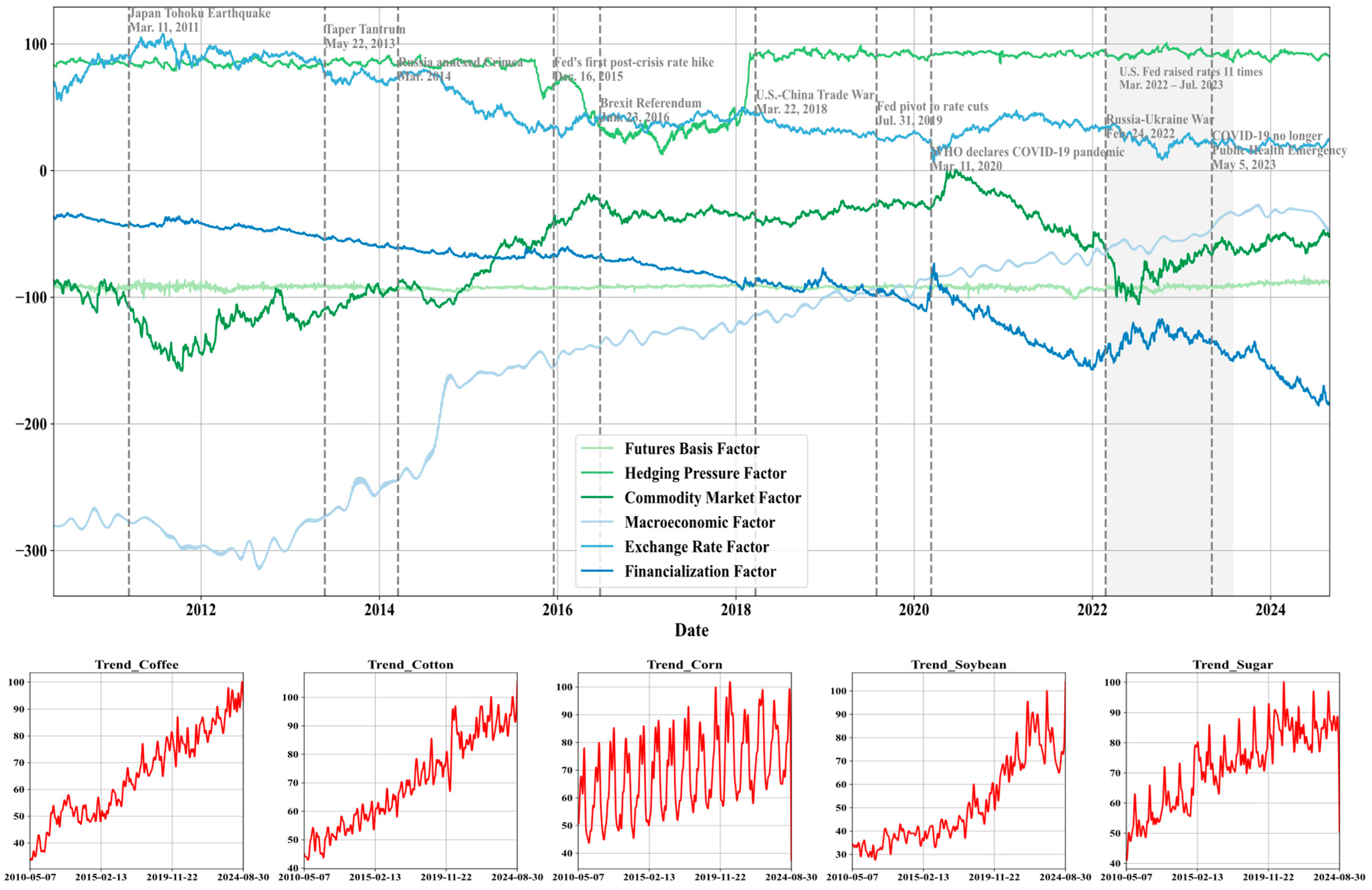
2.1.2. Construction of Seven Influencing Factors

To improve the economic interpretability of agricultural futures return predictions, this study incorporates seven key economic and financial factors. Existing research indicates that composite commodity indices impact specific agricultural prices, while macroeconomic conditions, exchange rates, financialization trends, and online attention also influence futures pricing. Building on the work of Guidolin and Pedio (2021) [44], we further include factors such as the futures basis and hedging pressure. Using rolling VMD processing, we select the factors with non-zero coefficients from these seven categories as predictive covariates. As shown in

Table 3. Description of economic and financial factors.

Type	Indicator	Frequency	Source
Futures basis factor	Spot price minus futures price	Daily	Wind
Hedging pressure factor	(Short hedge position—Long hedge position)/Total hedge position	Daily	Wind
Commodity market factor	Bloomberg Commodity	Daily	Investing database
	Dow Jones Commodity	Daily	Investing database
	MCX ICOMDEX Composite	Daily	Investing database
	S&P GSCI Commodity	Daily	Investing database
	TR_CC CRB Excess Return	Daily	Investing database
Macroeconomic factor	U.S. PPI	Monthly	Wind
	U.S. CPI	Monthly	Wind
	U.S. GDP	Quarterly	Wind
	U.S. M2	Monthly	Wind
	U.S. Unemployment Rate	Monthly	Wind
	Global Economic Policy Uncertainty Index	Monthly	Wind
Exchange rate factor	EUR to USD Exchange Rate	Daily	Wind
	USD to JPY Exchange Rate	Daily	Wind
	GBP to USD Exchange Rate	Daily	Wind
	USD to CHF Exchange Rate	Daily	Wind
	USD to CAD Exchange Rate	Daily	Wind
	AUD to USD Exchange Rate	Daily	Wind
	NZD to USD Exchange Rate	Daily	Wind
	USD to HKD Exchange Rate	Daily	Wind
	USD to SGD Exchange Rate	Daily	Wind
Financialization factor	NASDAQ Composite Index	Daily	Wind
	Standard and Poor’s 500 Index	Daily	Wind
	Dow Jones Industrial Average	Daily	Wind
	Federal Funds Rate	Daily	Wind
	U.S. 3 Month Treasury Yield	Daily	Wind
	U.S. 6 Month Treasury Yield	Daily	Wind
	U.S. 1 Year Treasury Yield	Daily	Wind
	U.S. 5 Year Treasury Yield	Daily	Wind
	U.S. 10 Year Treasury Yield	Daily	Wind
Attention factor	Google Trends	Weekly	https://trends.google.com (accessed on 20 February 2025)

Note: “Wind” refers to the Wind Financial Terminal by Wind Information Co., Ltd., Shanghai, China. “Investing database” refers to data obtained from Investing.com.

, these seven factors include:

(1) Futures basis factor: This is calculated by subtracting the futures price from the spot price of each agricultural product.

(2) Hedging pressure factor: This is calculated by dividing the difference between the short and long hedge positions for each futures contract by the total hedge position.

(3) Commodity market factor: This is derived using commodity indices from several major international exchanges, including Bloomberg Commodity, Dow Jones Commodity, MCX ICOMDEX Composite, S&P GSCI Commodity, and TR/CC CRB Excess Return.

(4) Macroeconomic factor: This is constructed using U.S. PPI, CPI, GDP, money supply (M2), unemployment rate, and the Global Economic Policy Uncertainty Index. Fluctuations in the macroeconomic environment have a significant impact on the supply, demand, and pricing of agricultural products.

(5) Exchange rate factor: This factor includes exchange rates for EUR/USD, USD/JPY, GBP/USD, USD/CHF, USD/CAD, AUD/USD, NZD/USD, USD/HKD, and USD/SGD.

(6) Financialization factor: It is composed of the three major U.S. stock indices and interest rates. The stock indices include the NASDAQ Composite Index, Standard and Poor’s 500 Index, and Dow Jones Industrial Average. The interest rates consist of the federal funds rate, as well as U.S. Treasury rates for three months, six months, one year, five years, and ten years. Commodity futures such as gold exhibit significant financialization attributes, making their prices highly sensitive to information from financial markets.

(7) Trend factor: This is measured using Google search trends based on commodity names as keywords. It reflects changes in public interest in specific commodities over time.

To address the challenges of high-dimensional data (e.g., curse of dimensionality, feature redundancy), this study uses a dynamic factors model (DFM) to consolidate variables into fewer, more meaningful factors [45,46]. Following Guidolin and Pedio (2021) [44], we group economically related variables (e.g., commodity indices for market impact; CPI and GDP as macroeconomic indicators) to maintain economic relevance while preserving data integrity. This seven factor framework reduces dimensionality, prevents underfitting, and enhances prediction accuracy.

Table 3 includes 46 variables in total. Among these, the futures basis factor and the hedging pressure factor each represent a single variable. The commodity market factor is derived from five commodity indices using the DFM method. The macroeconomic factor consists of six variables: the US PPI, US CPI, US GDP, US money supply (M2), US unemployment rate, and the Global Economic Policy Uncertainty Index. These indicators provide a clear reflection of changes in the global macroeconomic environment. The exchange rate factor, categorized as part of macroeconomic variables, uses nine currency pairs, while the financialization factor combines major stock indices, the Federal Funds Rate, and US Treasury bond rates. Finally, the attention factor is derived from Google Trends data for five agricultural futures, ensuring a comprehensive and refined model.

Table A1. Statistical description of factors.

Factor	Mean	Median	Std	Kurtosis	Skewness	Range	Min	Max
Futures basis factor	−91.9436	−91.9108	1.7426	3.5947	−0.3233	18.1792	−101.3845	−83.2053
Hedging pressure factor	80.8176	87.2311	19.4257	2.6197	−2.0012	88.0638	12.9354	100.9992
Commodity market factor	−65.8379	−58.4748	36.3452	−0.8837	−0.4316	158.8770	−158.2512	0.6258
Macroeconomic factor	−150.1331	−126.5533	89.9496	−1.2150	−0.4856	287.9777	−314.7341	−26.7565
Exchange rate factor	48.7258	39.4481	25.6298	−0.9473	0.6601	100.5115	7.4775	107.9890
Financialization factor	−88.2492	−79.6629	38.6009	−0.7622	−0.5674	152.1325	−185.6267	−33.4942
Trend_Coffee	65.2879	65.0328	16.4088	−1.0222	0.0860	66.5245	33.5933	100.1178
Trend_Cotton	70.2375	68.9863	15.7619	−1.2082	0.1593	62.5461	42.8412	105.3873
Trend_Corn	69.4271	68.4156	13.6862	−0.8334	0.1969	64.2815	37.5324	101.8139
Trend_Soybean	51.3910	43.9766	17.9223	−0.6405	0.7581	76.2414	27.5739	103.8153
Trend_Sugar	72.2897	73.7471	12.6377	−0.8995	−0.2932	59.0406	41.1065	100.1471

and Figure 2 summarize the seven constructed factors. The descriptive statistics highlight distinct patterns of volatility and kurtosis: the basis factor exhibits the lowest volatility but the highest kurtosis, indicating that its values are concentrated around the mean. In contrast, the hedging pressure factor shows higher volatility with a kurtosis less than 3. The commodity market, macroeconomic, exchange rate, and financialization factors all display elevated volatility, with the commodity market factor showing a pronounced negative skewness (heavy left tail). Among agricultural commodities, sugar, cotton, and corn attract significantly higher market attention, as reflected in their higher mean values.

Figure 2 illustrates key economic factors influencing agricultural futures. The futures basis factor shows a sharp increase following major events, such as the Japan Tohoku Earthquake and Fed rate hikes. Hedging pressure rises during significant trade disputes, such as the U.S.-China trade war, and geopolitical conflicts, such as the Russia-Ukraine war. The commodity market factor declines after disasters but rebounds during supply shocks, such as those triggered by natural disasters or geopolitical tensions. The macroeconomic factor shifts gradually in response to policy changes, such as Fed rate hikes or the economic impact of the COVID-19 pandemic. The exchange rate factor adjusts modestly to events such as Brexit and the ongoing Russia-Ukraine conflict. Lastly, the financialization factor spikes during economic crises, reflecting increased market activity and investor uncertainty.

Notably, all Google search indices experienced a sharp peak in early 2022. The Russia-Ukraine conflict led to tight supplies of natural gas and oil, fueling widespread concern over global energy and food crises. Rising energy and food prices worsened global inflation and heightened fears of an economic recession. Meanwhile, ongoing U.S.-China trade tensions disrupted global trade flows, particularly in commodities such as rare earths and semiconductors. As a result of these events, global Google search volumes for commodities surged significantly in 2022.

2.2. Methodology

2.2.1. Variational Mode Decomposition

VMD is a non-recursive model designed for concurrent extraction of modes from a multivariate input signal $x\left(t\right)$. VMD extends the classic Wiener filter to multiple adaptive bands, demonstrating effective practical results in signal decomposition.

VMD aims to extract a multivariate input signal $x\left(t\right)$ consisting of $C$ data channels into $K$ predefined multivariate modulation oscillation signals $u_k\left(t\right)=[u_1\left(t\right),u_2\left(t\right),\dots ,u_K(t\left)\right]$:

$$x\left(t\right)={\sum }_{k=1}^K{u}_k\left(t\right)$$

(1)

To ensure that each mode $u_k$ is primarily concentrated around a central frequency $w_k$, VMD employs two criteria for mode selection. The resulting constrained variational problem is formulated as:

$$\left\{\begin{array}{c}\underset{\left\{u_{k,c}\right\},\left\{w_k\right\}}{\min }\left\{\sum _{k=1}^K\sum _{c=1}^C{‖{\partial }_t\left[u_{+}^{k,c}\left(t\right)e^{-j{w}_{k}t}\right]‖}_2^2\right\},\\ s.t.\sum _{k=1}^K{u}_{k,c}\left(t\right)=x_c\left(t\right), c=\mathrm{1,2},\dots ,C,\end{array}\right.$$

(2)

where $u_{+}^{k,c}\left(t\right)$ denotes the analytic signal of the mode, $e^{-j{w}_{k}t}$ represents the frequency-shifting component, $\left\{u_{k,c}\right\}$ is the set of modulated oscillation signals in channel $c$, and ${\{w}_k\}$ are the center frequencies.

2.2.2. Least Absolute Shrinkage and Selection Operator (LASSO)

The LASSO regression model is a shrinkage estimation method that constrains variable contributions through a penalty function, compressing the regression coefficients of independent variables. Unlike traditional regression models, LASSO drives the coefficients of some variables toward zero by adjusting the penalty parameter $\lambda$, effectively screening out less influential variables and reducing model complexity.

The related linear regression model is established:

$$Y=X\mathrm{\beta }+\mathrm{\epsilon }$$

(3)

In Equation (3), $Y$ represents the $n\times 1$ dependent variable, which, in this study, can represent the Intrinsic Mode Function 1 (IMF1), IMF2, and residual components obtained from the decomposition of each sliding window. $X$ denotes the $n\times p$ four-dimensional data matrix, $\epsilon$ is the $n\times 1$ random error vector, and $\beta ={\left({\beta }_1,{\beta }_2,\dots ,{\beta }_p\right)}^{\mathrm{\top }}$ is the $p\times 1$ vector of regression coefficients, representing the parameters corresponding to each factor. By using the LASSO method to select variables, the parameters $\beta$ in Equation (3) can be obtained, such that the regression coefficients of some factors are shrunk to zero. The solution to the equation is as follows:

$$\beta =\arg \underset{\mathrm{\beta }}{\min }({‖Y-X\beta ‖}^2+\lambda {\sum }_{j=1}^p|{\beta }_j|)$$

(4)

In Equation (4), $\lambda {\sum }_{j=1}^p|{\beta }_j|$ represents the penalty term, where $\lambda >0$ is the tuning parameter that serves to screen variables. A larger $\lambda$ results in a stronger penalty, causing more variable coefficients to be compressed to zero, thereby achieving the purpose of dimensionality reduction for high-dimensional variables.

The tuning parameter $\lambda$ in the LASSO penalty is selected via fivefold cross-validation within each rolling window. A logarithmically spaced grid of 50 values between 10⁻⁴ and 10² is constructed to choose the $\lambda$ that minimizes the mean squared error on the held-out folds.

2.2.3. Mixed Ensemble Method

To improve the prediction accuracy and robustness for multi-commodity future price sequences, three types of ensemble learning methods are utilized based on previous research [47,48,49].

The first ensemble method is based on the evaluation of error metrics. It uses the predictive performance of individual models on the validation set as the criterion for determining weights, with the resulting weights detailed below:

$$w_j=X_j/{\sum }_{i=1}^n{X}_i$$

(5)

where $X$ include the inverse value of MSE, MAE, MAPE, U, ARV, and the value of DA. In Appendix A.3, this study has provided a detailed rationale for selecting Mean Square Error (MSE), Mean Absolute Error (MAE), Mean Absolute Percentage Error (MAPE), the U of Theil statistic (U), and Average Relative Variance (ARV) as evaluation metrics for forecasting performance. These metrics collectively offer a comprehensive assessment of the predictive capabilities of commodity price forecasting models. Therefore, in the first method of the mixed ensemble approach, these indicators are also employed as weighted components to evaluate the model’s performance.

The second type is based on decision tree methods, where the performance of each model in the validation set is assigned importance scores using Random Forest (RF), Gradient Boosting Decision Tree (GBDT), and Light Gradient Boosting Machine (LightGBM). These important scores serve as the basis for weight determination, with the weight calculation detailed below:

$$w_j={Feature Importance}_j/{\sum }_{i=1}^n{Feature Importance}_i$$

(6)

The third type relies on entropy-based predictions, employing three types of entropy metrics: Approximate Entropy (AE), Sample Entropy (SE), and Fuzzy Entropy (FE). A higher entropy value indicates greater uncertainty in the basic model’s predictions, while a lower entropy value suggests less uncertainty. Based on this, the weight calculation is as follows, where $X$ is the entropy value of AE, FE, and SE.

$$w_j=X_j^{-1}/{\sum }_{i=1}^n{X}_i^{-1}$$

(7)

The selection of error-based, decision tree–based, and entropy-based ensemble methods is motivated by the need to capture distinct facets of predictive performance and model diversity. Error-based weighting translates validation metrics directly into model importance scores, ensuring that models with superior empirical precision have greater influence. Decision tree–based weighting leverages the hierarchical feature-importance measures to reflect each learner’s structural contribution, capturing nonlinear interactions and complex dependencies. Entropy-based weighting employs various entropies to quantify the uncertainty inherent in each model’s output. By inversely weighting according to entropy, the framework systematically down-weights unstable or noisy predictors. These three paradigms embody complementary perspectives—error minimization, structural insight, and uncertainty management—with ensemble theory and the No Free Lunch theorem, maximizing robustness and generalizability in agricultural futures forecasting.

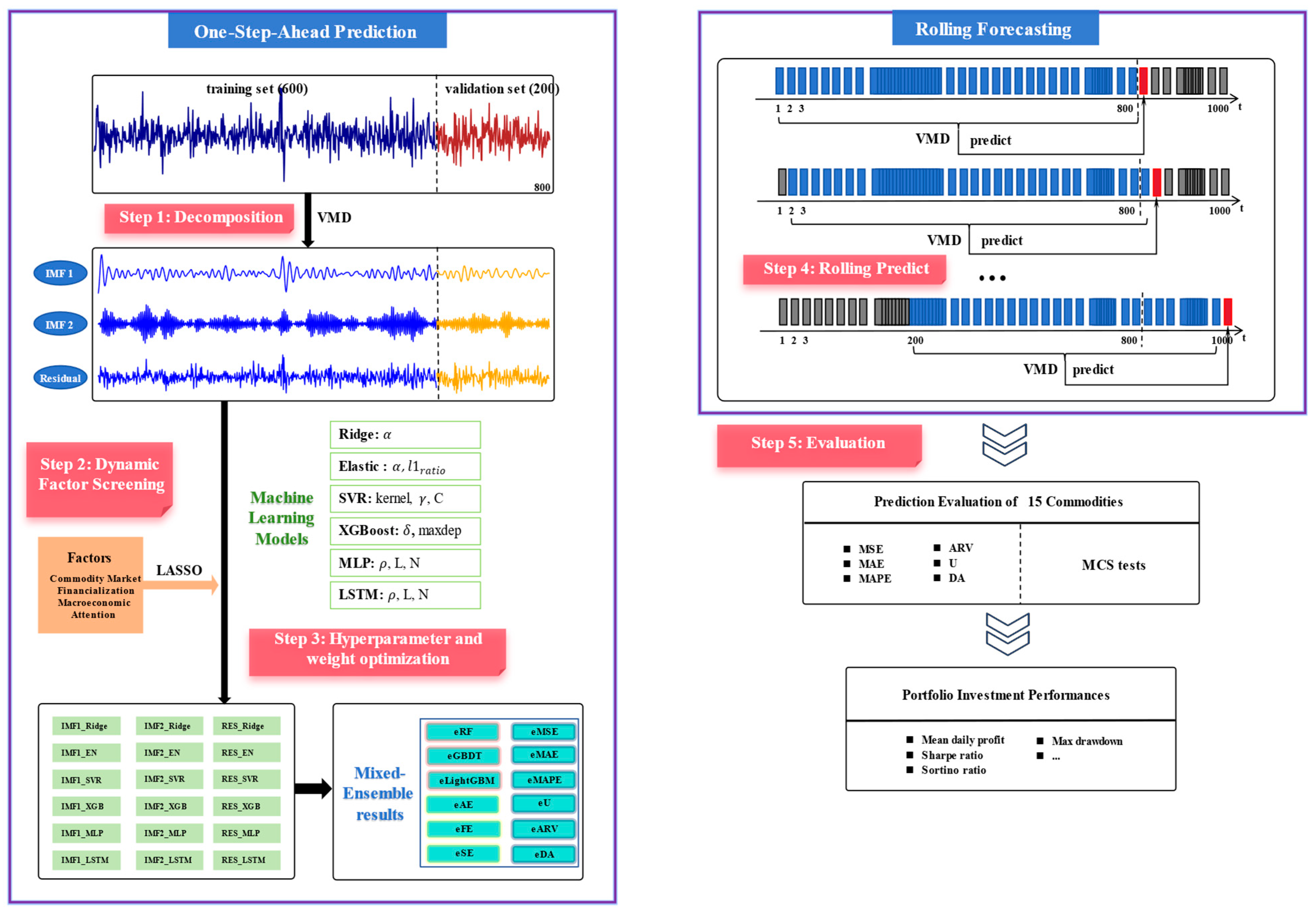
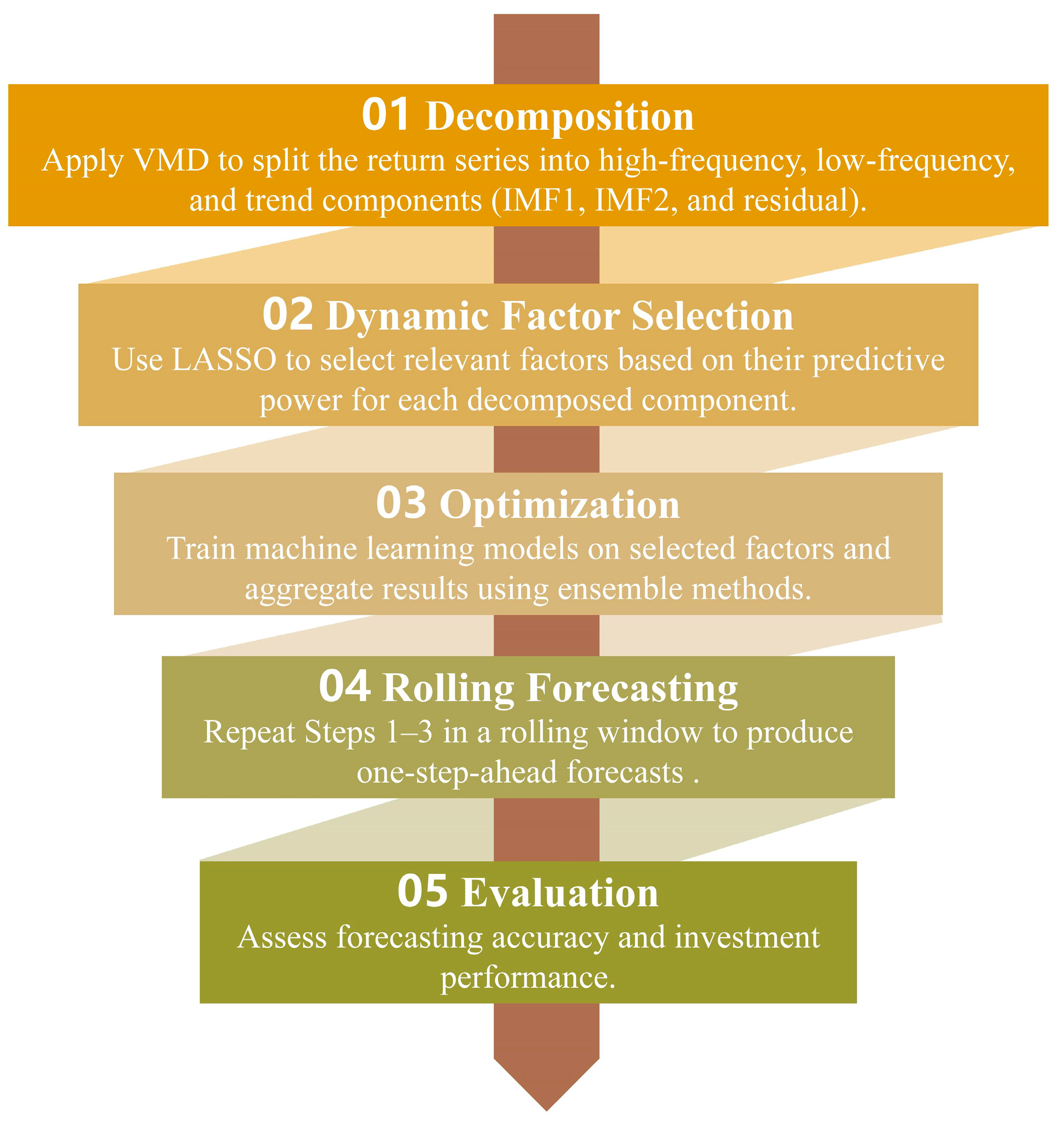
2.2.4. “Rolling VMD-LASSO-Mixed Ensemble” System for Commodity Returns Forecasting

This section provides a detailed description of the modeling process for the proposed “Rolling VMD-LASSO-Mixed Ensemble” forecasting framework. A simplified overview is presented in Figure 3, while a more detailed flowchart illustrating the full framework can be found in Appendix A.3 Figure A4.

In Steps 3 and 4, which focus on dynamic hyperparameter optimization for machine learning (as detailed in Section 3.2), several potential values are assigned to specific hyperparameters in each algorithm. During each sliding window, the training and validation sets are used to optimize these hyperparameters.

Step 1: Decomposition. The VMD method is applied with $k=2$ to decompose the original time series into two IMFs and a residual component, which represent the high-frequency, low-frequency, and trend components, respectively. Consistent with previous studies [50,51,52], we set the number of modes $k=2$ to produce high-frequency, low-frequency, and trend components that hold economic significance, as commonly observed in similar studies. These studies confirmed that two IMFs and a residual component balance decomposition granularity with computational efficiency, avoiding over-segmentation that can obscure economic signals.

Step 2: Dynamic factor screening. In this step, the LASSO method is applied to the three components obtained from the decomposition of each window. Factors are selected from the commodity market, macroeconomic, financialization, and attention factors constructed in Section 2.1.2. Only those factors with non-zero coefficients are retained.

Step 3: Hyperparameter and weight optimization. In this step, fitting is performed for the three components by combining their own lags with the factors selected in Step 2. The process includes hyperparameter optimization for machine learning and weight optimization for the mixed ensemble. Both fitting processes are completed within each 800-length window, using a 600-length training set and a 200-length validation set.

Step 4: Rolling forecasting. Steps 1 to 3 represent a one-step-ahead prediction process for a single window. To mitigate data leakage bias—a well-known issue in traditional full-sample decomposition methods—this study adopts a rolling-window forecasting framework. In this approach, Steps 1 to 3 are iteratively performed as the window advances forward by one observation at a time. For example, the first prediction uses commodity return data from the 1st to the 800th observation to forecast the 801st return; the second prediction uses data from the 2nd to the 801st to forecast the 802nd return. This recursive process continues until the 3736th return is forecasted. This procedure ensures that all forecasts are made strictly out-of-sample, thereby preserving the temporal integrity of the data and eliminating information leakage.

Step 5: Evaluation. This study evaluates the forecasting results of agricultural futures returns using a progressive approach. First, it compares the performance of the “Rolling VMD” framework with traditional univariate forecasting methods to highlight the advantages of the rolling-window VMD algorithm. Second, it compares the “Rolling VMD-LASSO” framework with the “Rolling VMD” framework to emphasize the impact of dynamic factor screening. Finally, the study compares the forecasting results of the “Rolling VMD-LASSO-Mixed Ensemble” framework with the “Rolling VMD-LASSO” framework to demonstrate the effectiveness of the ensemble method.

In this forecasting system, only a one-step-ahead prediction is required within each window, eliminating the need for multi-step predictions. This approach differs from the alternative method of dividing the entire sample into separate training and testing sets. Under the “Rolling VMD-LASSO-Mixed Ensemble” framework, as the date advances by one day, the data for day t + 1 becomes available. By sliding the window forward one step, the data for day t + 1 is included to predict the return for day t + 2. Since the model is designed to update and make predictions daily, performing multi-step-ahead predictions within each window would result in poorer performance compared to the rolling one-step-ahead prediction approach.

3. Results

This section first presents the LASSO-based dynamic factor selection results across components generated by rolling VM. Subsequently, it evaluates four distinct forecasting frameworks: the undecomposed benchmark system, the Rolling VMD prediction system, the Rolling VMD-LASSO system, and an integrated approach incorporating error-based, entropy-based, and decision tree-based ensemble methods applied to Rolling VMD-LASSO outputs. Each framework systematically integrates six machine learning algorithms: Ridge Regression (Ridge), Elastic Net (EN), Support Vector Regression (SVR), eXtreme Gradient Boosting (XGBoost), Multilayer Perceptron (MLP), and Long Short-Term Memory (LSTM) networks.

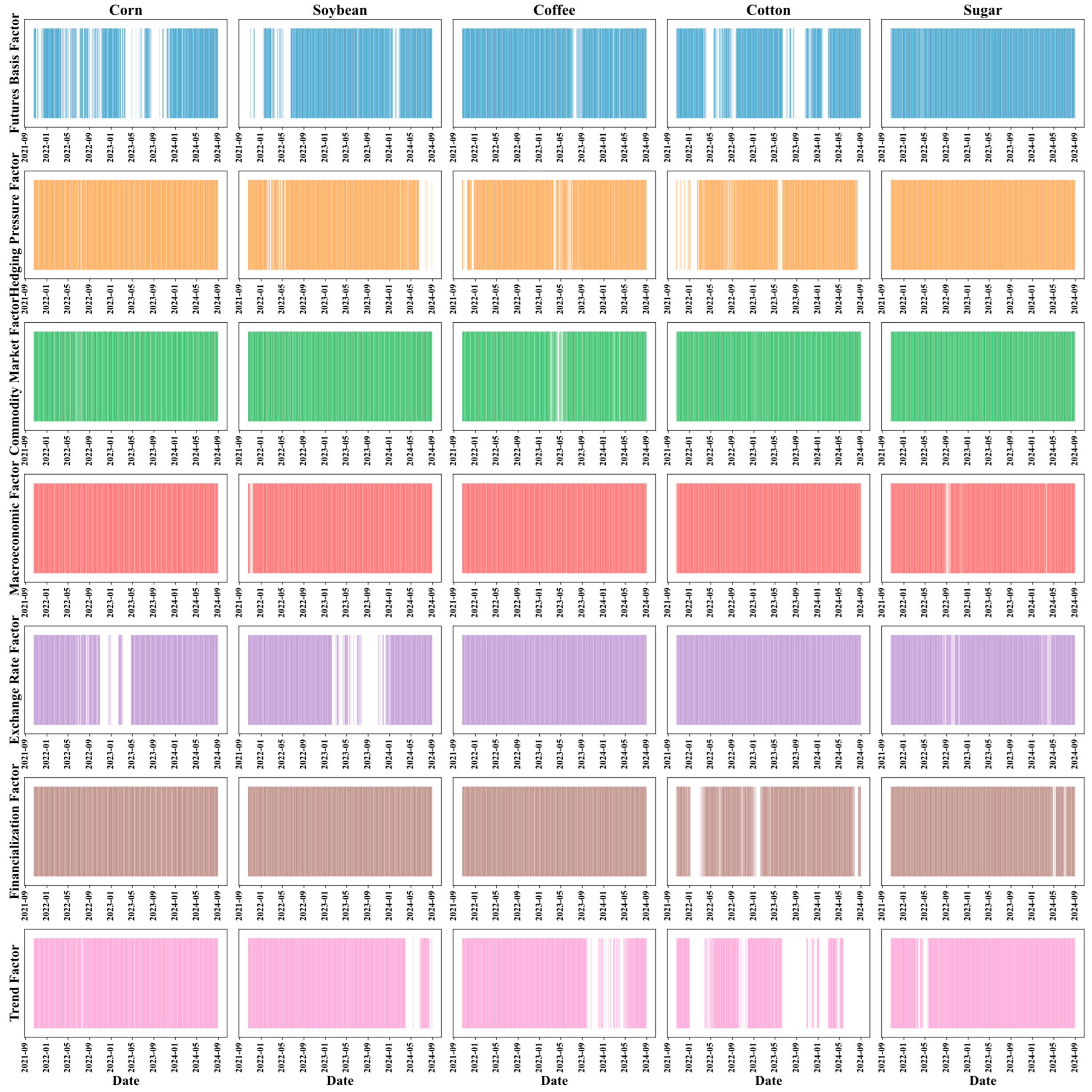
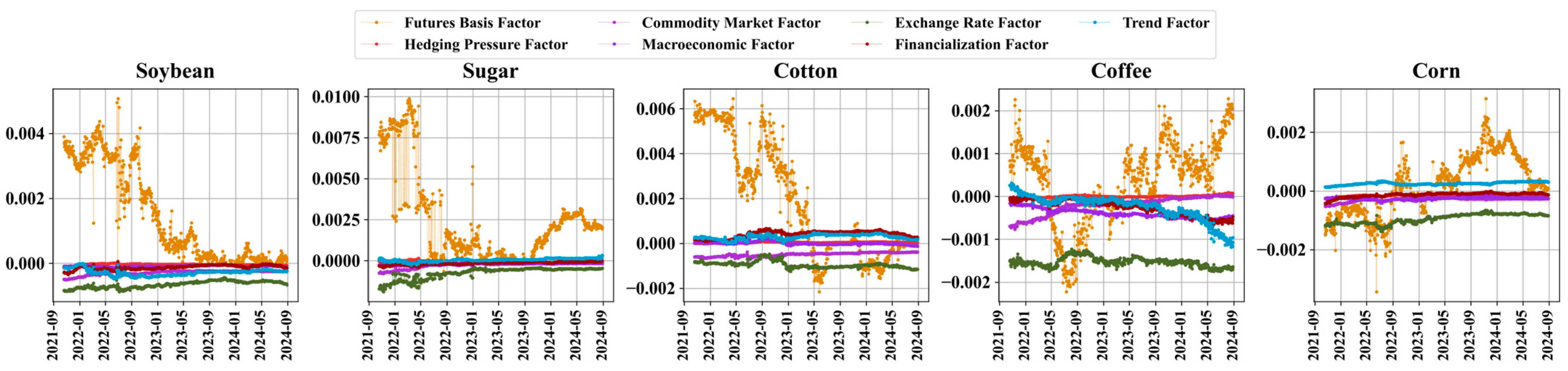
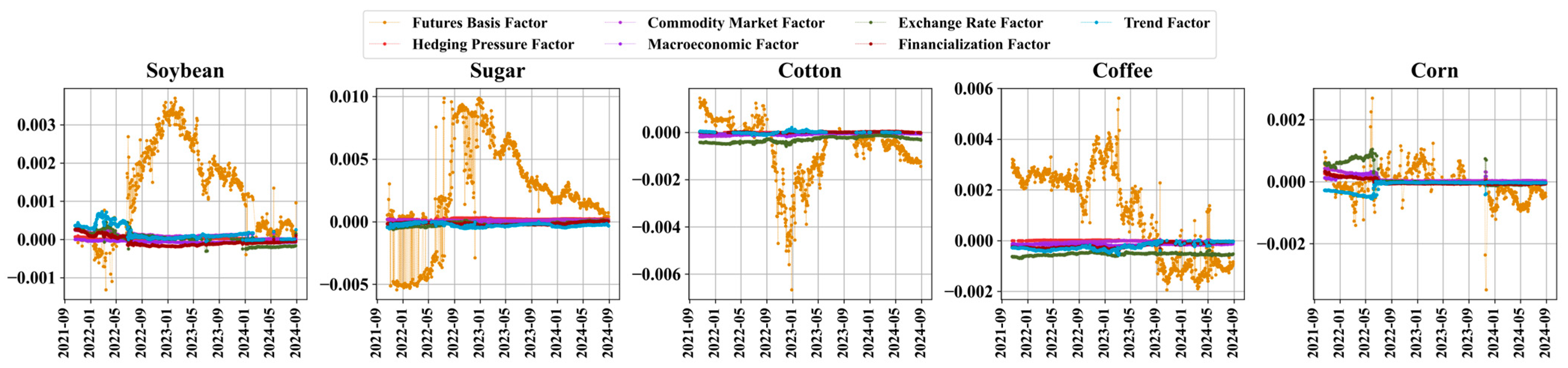
3.1. Result of LASSO Dynamic Factors Screening

On each sliding window, this study applies the LASSO method (defined in Section 2.2.2) to select from the seven factors constructed in Section 2.1.2, retaining only those with non-zero coefficients. This process, repeated across each sliding window, results in dynamic factor selection.

Figure A1, Figure A2 and Figure A3 illustrate the time-varying factors screened by the three components across 2936 sliding windows, where blue denotes the futures basis factor, green represents the commodity market factor, purple signifies the exchange rate factor, pink stands for the attention factor, orange indicates the hedging pressure factor, red corresponds to the macroeconomic factor, and brown embodies the financialization factor. The vertical lines of different colors on the horizontal axis represent whether or not the impact factor has been selected by the LASSO method for the model prediction at the current time point under the three components (high, low, and residual).

Figure A5, Figure A6 and Figure A7 in the Appendix A.3 show the time-varying coefficients of seven key factors influencing agricultural commodity futures returns, revealing their different pricing mechanisms through the signs and magnitudes of the coefficients. The hedge pressure factor has a significant positive impact on the high-frequency component of agricultural futures returns, indicating that hedge activities in the futures market amplify short-term price volatility. Investors and producers typically hedge through the futures market to lock in future prices, and as hedge demand increases, trading volume in the futures market rises, leading to intensified price fluctuations in the short-term. Due to rapid changes in imports and exports, the impact of exchange rate factors on the high-frequency component switches between positive and negative values. The initial increase in online attention reflects growing interest among market participants in agricultural futures; however, over time, excessive information and the market’s gradual digestion of it may lead to stabilization in price volatility. As a result, the influence of online attention on the high-frequency component of futures returns begins to weaken.

Since agricultural futures are a segment of the global commodity futures market, commodity indices have a lasting and stable impact on the low-frequency component of agricultural futures returns. The influence of macroeconomic factors on the low-frequency component shows cyclical fluctuations consistent with economic cycles, indicating that macroeconomic factors affect the long-term price trend of agricultural futures. During economic expansion, increased consumer income and strong demand lead to higher agricultural demand, which drives up agricultural prices. However, the impact of macroeconomic factors is gradual and exhibits time lags, thus influencing the long-term prices of agricultural futures. The above analysis preliminarily suggests that short-term price movements of agricultural futures are driven by trading behaviors, while long-term trends are determined by macroeconomic conditions and market fundamentals.

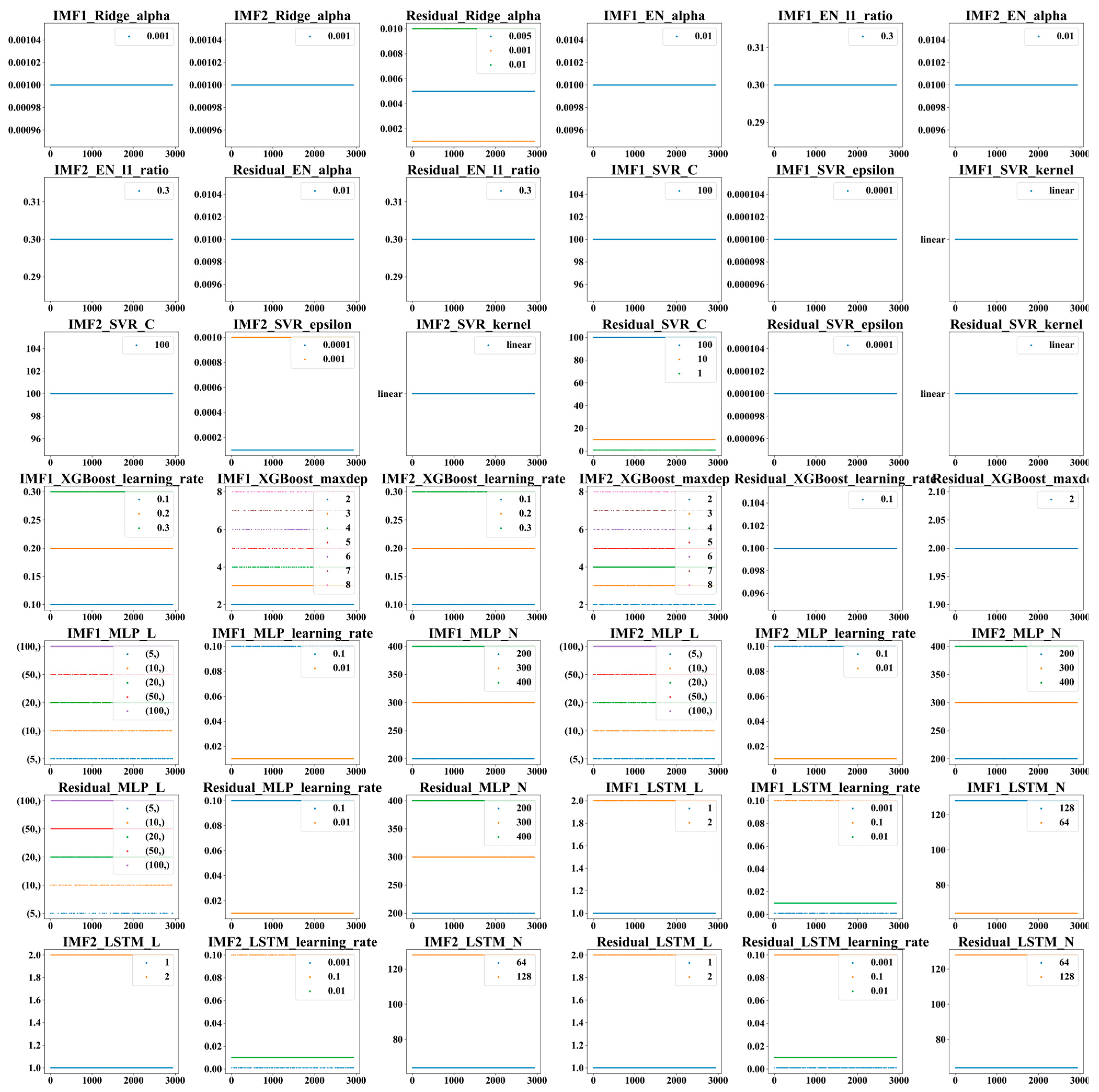
3.2. Results of Hyperparameter Tuning

Initially, a parameter pool is defined, as shown in

Table A2. Hyperparameters pool for grid search.

Algorithm	Parameter	Value	Algorithm	Parameter	Value
Ridge	alpha	(0.1, 0.01, 0.001, 0.005)	EN	alpha	(0.1, 0.01, 0.001)
SVR	kernel	(‘linear’, ’rbf’)		${l1}_{ratio}$	(0.3, 0.5, 0.7)
	epsilon	($10, 1, 0.1, 0.01, 0.001, 0.0001$)	XGBoost	learning_rate	(0.1, 0.2, 0.3)
	C	(1 × 10−1, 1, 10, 100, 1000)		max_depth	(2, 3, 4, 5, 6, 7, 8)
LSTM	learning rate	(0.1, 0.01, 0.001)	MLP	learning_rate	(0.1, 0.01, 0.001)
	L	(1, 2)		L	(5, 10, 20, 50, 100)
	N	(64, 128)		N	(200, 300, 400)

. Parameter tuning is conducted for each decomposed component of all agricultural futures. Given the dynamic nature of commodity markets, the optimal parameters for each rolling window vary over time. The tuning procedure is repeated in each rolling window for 2936 times. The parameters that yield the best MSE performance are deemed optimal.

Figure A8 in the Appendix A.3 presents the hyperparameter tuning results across 2936 soybean futures windows, revealing distinct patterns for IMF1, IMF2, and residual term predictions. For IMF1, Ridge (α = 0.001) and EN (α = 0.01) maintain constant regularization, while SVR shows stable kernel parameters. XGBoost’s learning rate varies between 0.1 and 0.3 across windows. Similar learning rate variation appears in IMF2 prediction. For residuals, LSTM demonstrates strong hyperparameter preferences: sequence length (L = 1) in 74.7% of windows, learning rate (0.01) in 54.9%, and neuron count (N = 64) in 67.8% of cases, indicating model stability in residual term prediction. While Figure A8 focuses on soybeans as a representative example, the same hyperparameter tuning procedure was applied to all five agricultural futures. The results across the other commodities (coffee, cotton, corn, and sugar) exhibit similar parameter stability and patterns, and are therefore not presented separately due to space considerations.

3.3. Prediction Results

3.3.1. Comparative Analysis of the “Rolling VMD” Forecasting System and Traditional Systems

Section 3.3.1, Section 3.3.2 and Section 3.3.3 compare the performance of forecast combination models across multiple systems. For example, in Section 3.3.2, the forecasting effectiveness is compared between the “Rolling VMD-LASSO” system and the “Rolling VMD” system. However, the machine learning model is held constant during the comparison, meaning the combined model using the Ridge algorithm in the “Rolling VMD-LASSO” system is compared to the combined model using the Ridge algorithm in the “Rolling VMD” system. Similarly, the comparison in Section 3.3.3 between the “Rolling VMD-LASSO-Mixed Ensemble” system and the “Rolling VMD-LASSO” system is also a comparison of combined models.

Figure 4 shows that the “Rolling VMD” forecasting framework outperforms in predicting the returns of five commodity futures, using six machine learning methods. The comparison is based on the MSE metric, where lower values indicate better forecasting performance. For example, in predicting soybean futures returns, vRidge (1.40 × 10⁻⁴) outperforms Ridge (1.49 × 10⁻⁴), vEN (1.33 × 10⁻⁴) outperforms EN (1.49 × 10⁻⁴), vSVR (1.42 × 10⁻⁴) outperforms SVR (1.49 × 10⁻⁴), vXGBoost (1.34 × 10⁻⁴) outperforms XGBoost (1.46 × 10⁻⁴), vLSTM (1.32× 10⁻⁴) outperforms LSTM (1.49 × 10⁻⁴), and the prediction ability of vMLP (1.49 × 10⁻⁴) and MLP (1.49 × 10⁻⁴) is equal. In predicting corn futures returns, vRidge (2.06 × 10⁻⁴) outperforms Ridge (2.14 × 10⁻⁴), vEN (1.94 × 10⁻⁴) outperforms EN (2.14× 10⁻⁴), vSVR (1.94 × 10⁻⁴) outperforms SVR (2.17 × 10⁻⁴), vXGBoost (1.92 × 10⁻⁴) outperforms XGBoost (2.14 × 10⁻⁴), vLSTM (2.19 × 10⁻⁴) outperforms LSTM (2.33 × 10⁻⁴), and vMLP (2.15 × 10⁻⁴) outperforms MLP (2.23 × 10⁻⁴). These results suggest that the decomposition-based “Rolling VMD” framework improves predictive accuracy compared to the traditional univariate system.

Figure 4 (rows 2–6) compares the performance between the “Rolling VMD” framework and the univariate prediction framework across five metrics: MAE, MAPE, DA, ARV, and U. With the exception of MAPE, the “Rolling VMD” framework demonstrates superior performance over the univariate framework for most agricultural commodity futures. This advantage holds true across multiple machine learning algorithms in terms of MAE, DA, ARV, and U metrics.

Table 4. MCS results between the “Rolling VMD” framework and the traditional system.

	Panel A: TR					Panel B: TMAX
Commodity	Coffee	Cotton	Corn	Soybean	Sugar	Coffee	Cotton	Corn	Soybean	Sugar
Ridge	0.914(5)	0.000 (10)	0.006 (11)	0.000 (8)	0.937 (4)	0.947 (5)	0.215 (10)	0.040 (11)	0.004 (8)	0.899 (4)
EN	0.110 (11)	0.041 (5)	0.005 (12)	0.000 (7)	0.101 (11)	0.332 (11)	0.215 (5)	0.019 (12)	0.004 (7)	0.381 (11)
SVR	0.002 (12)	0.000 (11)	0.019 (7)	0.000 (12)	0.050 (12)	0.242 (12)	0.215 (11)	0.971 (7)	0.000 (12)	0.381 (12)
XGBoost	0.545 (9)	0.041 (6)	0.007 (10)	0.000 (10)	0.937 (3)	0.676 (9)	0.215 (6)	0.104 (10)	0.002 (10)	0.899 (3)
MLP	0.545 (8)	0.000 (12)	0.019 (8)	0.000 (11)	0.329 (7)	0.900 (8)	0.183 (12)	0.568 (8)	0.000 (11)	0.418 (7)
LSTM	0.858 (6)	0.007 (9)	0.026 (5)	0.001 (6)	0.269 (8)	0.900 (6)	0.215 (9)	0.999 (5)	0.190 (6)	0.381 (8)
vRidge	1.000 (1)	0.041 (7)	0.015 (9)	0.000 (9)	1.000 (1)	1.000 (1)	0.215 (7)	0.568 (9)	0.002 (9)	1.000 (1)
vEN	0.950 (3)	1.000 (1)	0.874 (2)	0.875 (2)	0.329 (6)	0.949 (3)	1.000 (1)	0.999 (2)	0.887 (2)	0.424 (6)
vSVR	0.950 (4)	0.041 (4)	0.874 (3)	0.003 (5)	0.937 (5)	0.949 (4)	0.215 (4)	0.999 (3)	0.412 (5)	0.885 (5)
vXGBoost	0.706 (7)	0.067 (3)	1.000 (1)	0.254 (4)	0.143 (9)	0.900 (7)	0.894 (3)	1.000 (1)	0.412 (4)	0.381 (9)
vMLP	0.950 (2)	0.013 (8)	0.085 (4)	0.721 (3)	0.937 (2)	0.949 (2)	0.215 (8)	0.999 (4)	0.609 (3)	0.899 (2)
vLSTM	0.404 (10)	0.460 (2)	0.026 (6)	1.000 (1)	0.142 (10)	0.676 (10)	0.894 (2)	0.999 (6)	1.000 (1)	0.381 (10)

Note: TR refers to the trace statistic, and TMAX refers to the maximum statistic used in the MCS test.

presents the Model Confidence Set (MCS) test results comparing the two forecasting frameworks. Taking the TR metric as an example, the model ranking results demonstrate the clear superiority of the “Rolling VMD” framework. Specifically, the average rankings are as follows: for coffee, 4.5 (“Rolling VMD”) versus 8.5 (univariate framework); for cotton, 4.17 versus 9.5; for corn, 4.17 versus 9.5; for soybean, 4 versus 9; and for sugar, 5.5 versus 7.5. These MCS test results consistently validate the superior predictive performance of the “Rolling VMD” framework across all examined agricultural commodities.

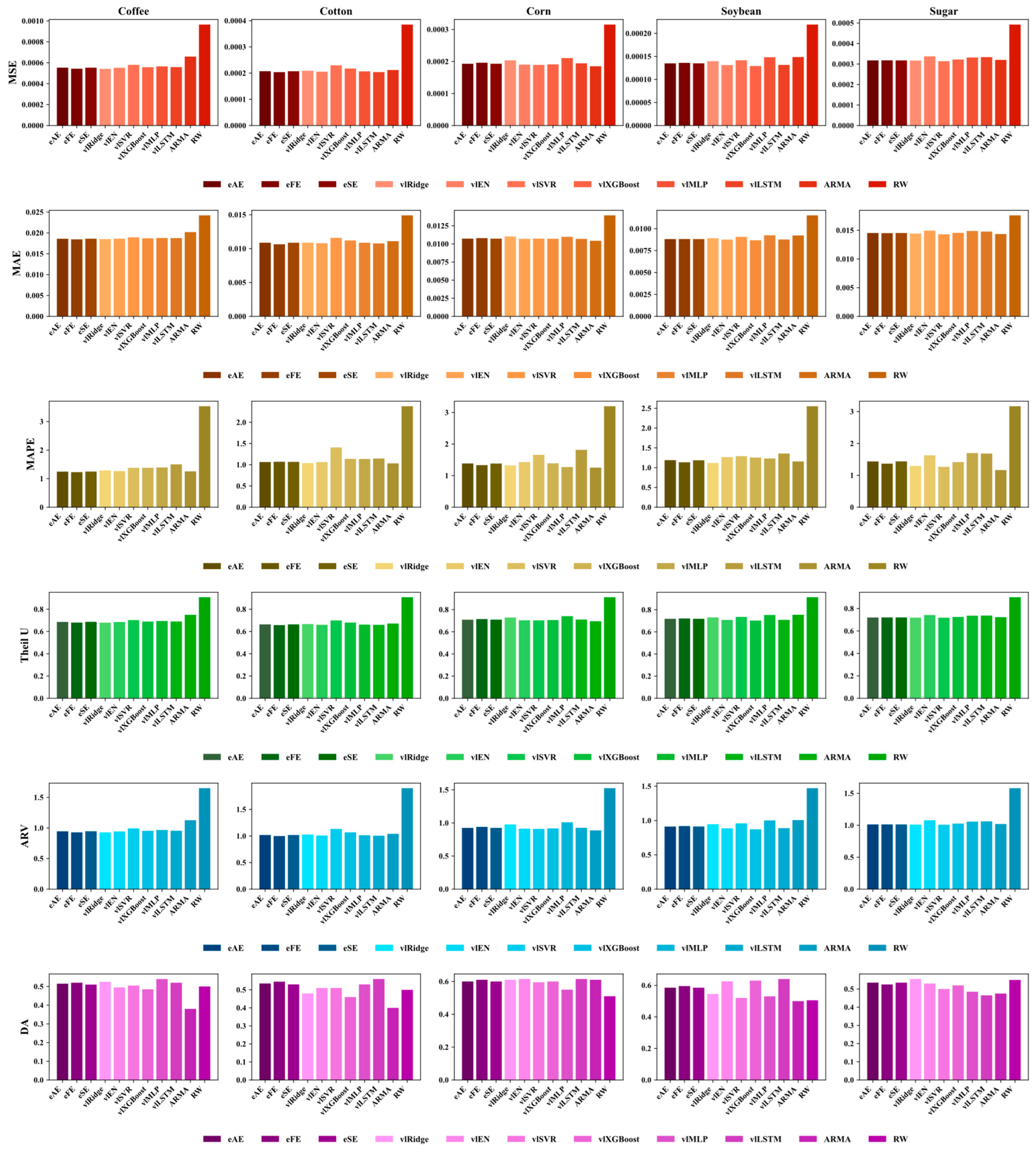
3.3.2. Comparative Analysis of the “Rolling VMD-LASSO” Forecasting System and “Rolling VMD” Systems

In Section 3.3.2, this study will discuss whether incorporating the LASSO dynamic factor selection method into the “Rolling VMD” prediction framework can lead to improved prediction performance compared to the “Rolling VMD” framework alone. To address this, factors affecting the three components obtained from each sliding window are selected from the futures basis factor, hedging pressure factor, commodity market factor, macroeconomic factor, exchange rate factor, financialization factor, as established in Section 2.1.2.

Figure 5 presents the MSE values for the prediction results of six models across two frameworks, based on the five agricultural futures return datasets. For ease of comparison, models using the “Rolling VMD” method are labeled with the prefix “v”, while models using the “Rolling VMD-LASSO” method are labeled with the prefix “vl”. For example, vEN represents the MSE results using the Elastic Net algorithm within the “Rolling VMD” framework, and vlEN represents the MSE results using the Elastic Net algorithm within the “Rolling VMD-LASSO” framework.

Figure 5 demonstrates that the “Rolling VMD-LASSO” forecasting framework outperforms its “Rolling VMD” counterpart in at least four models across several agricultural commodity futures. Taking coffee futures as an example, vlRidge (5.42 × 10⁻⁴) shows superior performance to vRidge (5.67 × 10⁻⁴), vlElastic Net (5.52 × 10⁻⁴) surpasses vElastic Net (5.83 × 10⁻⁴), vlSVR (5.80 × 10⁻⁴) exceeds vSVR (5.90 × 10⁻⁴), vlXGBoost (5.58 × 10⁻⁴) performs better than vXGBoost (5.79 × 10⁻⁴), and vlLSTM (5.59 × 10⁻⁴) achieves lower errors than vLSTM (6.08 × 10⁻⁴).

Figure 5 (rows 2–6) presents a comprehensive comparison of the “Rolling VMD-LASSO” and “Rolling VMD” frameworks across MAE, MAPE, DA, ARV, and U metrics. While the “Rolling VMD-LASSO” framework generally demonstrates superior performance in most cases, there exist specific instances where it underperforms relative to the “Rolling VMD” approach. In coffee futures prediction, vlSVR produces higher U values than vSVR, while vlMLP achieves lower DA values than vMLP. For corn futures, both vlLSTM and vlXGBoost show higher MAPE values compared to their “Rolling VMD” counterparts. Similarly, in cotton futures, vlRidge and vlSVR generate higher MSE values than vRidge and vSVR, respectively. However, these exceptions constitute a relatively small proportion of cases, and the “Rolling VMD-LASSO” framework maintains better overall accuracy performance across the majority of error metrics examined.

Table 5. MCS results between the “Rolling VMD-LASSO” framework and the “Rolling VMD” system.

	Panel A: TR					Panel B: TMAX
Commodity	Coffee	Cotton	Corn	Soybean	Sugar	Coffee	Cotton	Corn	Soybean	Sugar
vRidge	0.953 (3)	0.022 (12)	0.867 (5)	0.004 (11)	1.000 (1)	0.863 (3)	0.030 (12)	0.933 (5)	0.133 (11)	1.000 (1)
vEN	0.001 (12)	0.380 (6)	0.149 (7)	0.020 (6)	0.364 (7)	0.045 (12)	0.871 (6)	0.933 (7)	0.305 (6)	0.491 (7)
vSVR	0.001 (11)	0.154 (7)	0.000 (12)	0.006 (9)	0.115 (11)	0.087 (11)	0.871 (7)	0.006 (12)	0.179 (9)	0.225 (11)
vXGBoost	0.073 (9)	0.754 (5)	0.005 (10)	0.006 (10)	0.177 (10)	0.767 (9)	0.871 (5)	0.014 (10)	0.133 (10)	0.225 (10)
vMLP	0.892 (5)	0.154 (8)	0.867 (6)	0.056 (5)	0.711 (2)	0.824 (5)	0.162 (8)	0.933 (6)	0.305 (5)	0.854 (2)
vLSTM	0.019 (10)	0.026 (11)	0.867 (4)	0.150 (3)	0.184 (9)	0.229 (10)	0.090 (11)	0.933 (4)	0.464 (3)	0.321 (9)
vlRidge	0.953 (2)	0.029 (10)	0.061 (8)	0.000 (12)	0.711 (3)	0.863 (2)	0.162 (10)	0.873 (8)	0.133 (12)	0.854 (3)
vlEN	0.709 (7)	0.908 (2)	0.915 (2)	0.150 (4)	0.711 (6)	0.824 (7)	0.871 (2)	0.933 (2)	0.464 (4)	0.840 (6)
vlSVR	0.850 (6)	1.000 (1)	0.001 (11)	0.020 (7)	0.711 (5)	0.824 (6)	1.000 (1)	0.008 (11)	0.247 (7)	0.840 (5)
vlXGBoost	0.953 (4)	0.908 (3)	0.036 (9)	0.150 (2)	0.711 (4)	0.863 (4)	0.871 (3)	0.176 (9)	0.464 (2)	0.840 (4)
vlMLP	1.000 (1)	0.111 (9)	0.915 (3)	0.017 (8)	0.018 (12)	1.000 (1)	0.162 (9)	0.933 (3)	0.179 (8)	0.086 (12)
vlLSTM	0.617 (8)	0.816 (4)	1.000 (1)	1.000 (1)	0.194 (8)	0.767 (8)	0.871 (4)	1.000 (1)	1.000 (1)	0.321 (8)

Note: See Table 4 for definitions of TR and TMAX.

presents the Model Confidence Set (MCS) test results comparing the “Rolling VMD-LASSO” and “Rolling VMD” frameworks. Using the TR metric as an example, the model ranking results clearly demonstrate the superior performance of “Rolling VMD-LASSO”. For coffee futures, “Rolling VMD-LASSO” achieves an average ranking of 4.67 compared to 8.33 for “Rolling VMD”. Similarly for cotton, the average rankings are 4.83 versus 8.17. The pattern continues with corn (5.67 vs. 7.33), soybean (5.67 vs. 7.33), and sugar (6.33 vs. 6.67). These consistent results across all examined commodities validate the significant advantage of the “Rolling VMD-LASSO” framework over its “Rolling VMD” counterpart in predictive performance.

3.3.3. Comparative Analysis of the “Rolling VMD-LASSO-Mixed Ensemble” Forecasting System and “Rolling VMD-LASSO” Systems

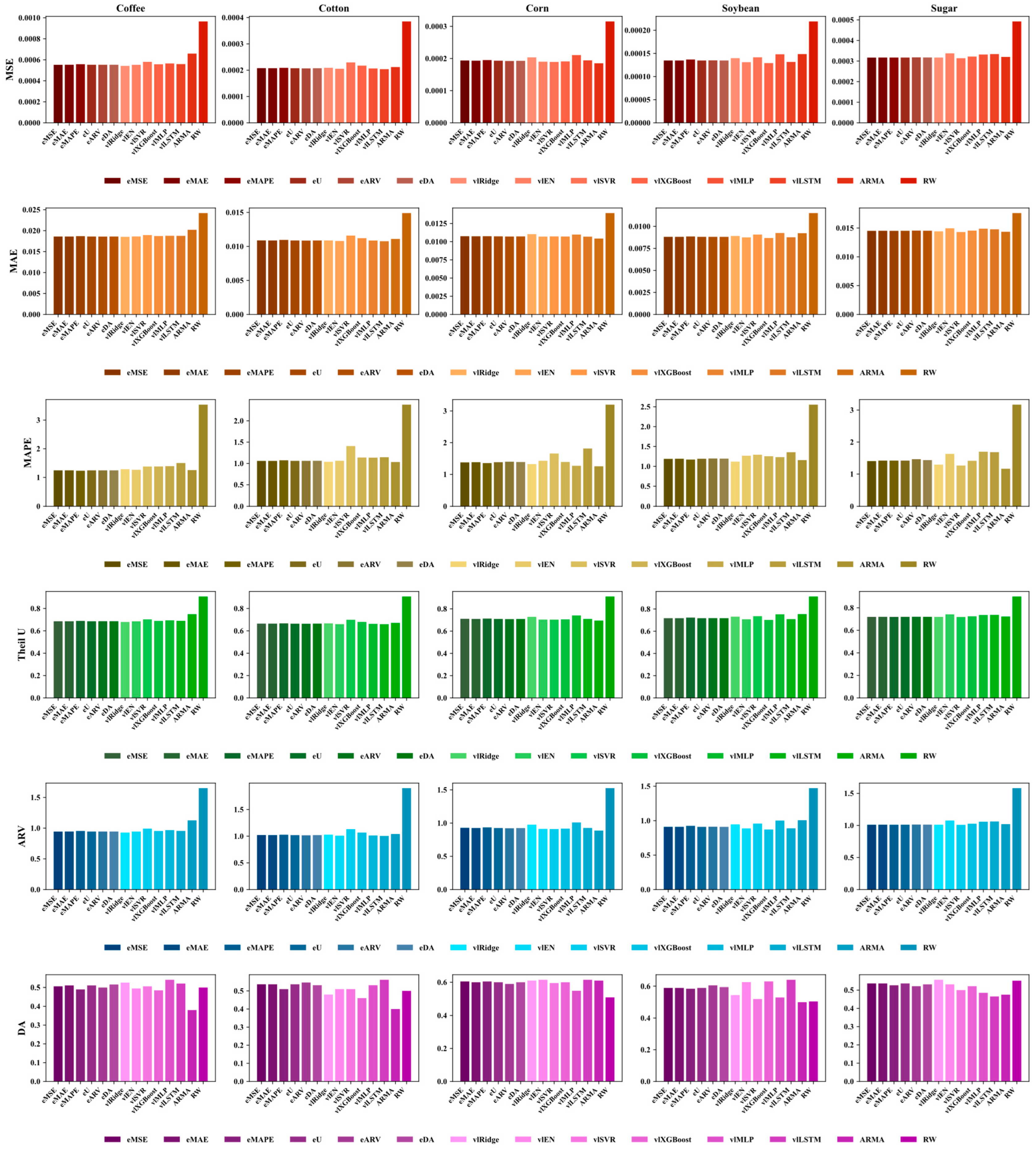
Prediction Results of the Ensemble Model Based on Error Metrics and Entropy Values

Finally, this study aims to discuss whether the mixed ensemble method presented in Section 2.2.3, including error-based ensemble, entropy-based ensemble, and decision tree-based ensemble, can integrate the strengths of six machine learning algorithms to further improve the prediction accuracy of commodity futures return within the “Rolling VMD-LASSO” framework.

Figure A9 in the Appendix A.3 compares the error-based ensemble “Rolling VMD-LASSO” framework with the standard “Rolling VMD-LASSO” approach across six error metrics while also, including benchmark models (ARMA and RW) commonly used in previous studies for comparison. On average, the error-based ensemble achieves improvements of 1.67% in MSE, 0.81% in MAE, 6.69% in MAPE, 0.86% in U, 1.78% in ARV, and 1.88% in DA. However, these gains are relatively limited and lack consistency. Across all five agricultural commodities examined (coffee, cotton, corn, soybean, and sugar), the ensemble fails to outperform the standard version in at least three of the base learners per commodity. This limitation may stem from the static and purely performance-based nature of the weighting scheme, where model weights are derived solely from inverse validation errors. While this method captures overall accuracy, it lacks sensitivity to the contextual relevance of individual predictors and cannot account for the structural contributions of each model or the dynamic behavior of different factors over time.

Figure A10 in the Appendix A.3 presents a comparative analysis of MSE metrics between the entropy-based “Rolling VMD-LASSO-Mixed Ensemble” framework and the standard “Rolling VMD-LASSO” framework. The models eAE, eFE, and eSE represent the entropy-based ensemble variants (as detailed in Section 2.2.3) corresponding to three distinct entropy measures. On average, this method achieves improvements of 1.96% in MSE, 1.02% in MAE, 7.36% in MAPE, 0.95% in U, 1.98% in ARV, and 2.46% in DA compared to the baseline. Nevertheless, these improvements are not uniformly observed. Figure A10 reveals that for four out of the five agricultural commodity futures examined, the standard “Rolling VMD-LASSO” framework outperforms the entropy-based ensemble approach in at least three machine learning algorithms. This finding indicates that the entropy-based “Rolling VMD-LASSO-Mixed Ensemble” fails to establish a competitive advantage. More notably, in terms of MAPE metrics for corn, cotton, soybean, and sugar futures, the entropy-based ensemble demonstrates inferior performance compared to even the basic ARMA benchmark model. This underperformance may be due to the entropy-based weights reflecting uncertainty rather than predictive power. Since high entropy signals unstable or less confident predictions, inversely weighting based on entropy might disproportionately favor models with low variance rather than high accuracy.

Prediction Results of the Decision Tree-Based Ensemble Model

Figure 6 presents a comparison of error metrics between the decision tree-based “Rolling VMD-LASSO-Mixed Ensemble” framework and the “Rolling VMD-LASSO” framework. Here, eRF, eGBDT, and eLightGBM denote ensemble models employing three distinct decision tree methods. As illustrated in Figure 6, for each agricultural commodity futures variety, the decision tree-based “Rolling VMD-LASSO-Mixed Ensemble” framework outperforms the alternative in at least four out of the six error metrics. For instance, in the case of sugar forecasting, eRF, eGBDT, and eLightGBM achieve lower MSE and MAE values compared to all five models under the “Rolling VMD-LASSO” framework, while surpassing four models in terms of MAPE. On average, the decision tree–based ensemble outperforms the standard “Rolling VMD-LASSO” framework by 1.98% in MSE, 0.96% in MAE, 1.28% in MAPE, 2.55% in Theil’s U, and 4.18% in DA. It also consistently surpasses the ARMA and RW benchmark models across all commodities.

These results suggest that the decision tree–based ensemble method offers a more reliable and generalizable integration of model outputs. Unlike the error- or entropy-based approaches, which assign weights based solely on validation accuracy or output uncertainty, the decision tree–based method assigns weights based on feature importance scores, capturing the structural contribution of each model in terms of how effectively it utilizes different predictive variables. The weight determination process is more context-aware and better aligned with the model’s internal decision logic. This allows the framework to maintain interpretability while enhancing robustness across different commodity types and forecasting horizons, especially in the presence of non-stationary and heterogeneous market dynamics.

Table 6. MCS results between the decision tree mixed ensemble models and the “Rolling VMD-LASSO” system and the “Rolling VMD-LASSO” system.

	Panel A: TR					Panel B: TMAX
Commodity	Coffee	Cotton	Corn	Soybean	Sugar	Coffee	Cotton	Corn	Soybean	Sugar
RW	0.333 (10)	0.000 (11)	0.000 (11)	0.000 (10)	0.001 (10)	0.556 (10)	0.000 (11)	0.000 (11)	0.000 (10)	0.001 (10)
ARMA	0.000 (11)	0.001 (10)	0.000 (10)	0.000 (11)	0.000 (11)	0.000 (11)	0.009 (10)	0.002 (10)	0.000 (11)	0.000 (11)
vlRidge	0.706 (8)	0.499 (5)	0.000 (9)	0.008 (7)	0.909 (5)	0.602 (8)	0.566 (5)	0.003 (9)	0.009 (7)	0.931 (5)
vlElastic	0.883 (5)	0.499 (6)	0.979 (2)	0.028 (5)	0.909 (3)	0.824 (5)	0.524 (6)	0.932 (2)	0.014 (5)	0.931 (3)
vlSVR	1.000 (1)	0.268 (8)	0.979 (5)	0.000 (8)	0.779 (8)	1.000 (1)	0.524 (8)	0.932 (5)	0.003 (8)	0.898 (8)
vlXGBoost	0.635 (9)	0.477 (7)	1.000 (1)	1.000 (1)	0.059 (9)	0.602 (9)	0.524 (7)	1.000 (1)	1.000 (1)	0.117 (9)
vlMLP	0.868 (6)	1.000 (1)	0.071 (7)	0.000 (9)	0.909 (2)	0.824 (6)	1.000 (1)	0.618 (7)	0.002 (9)	0.931 (2)
vlLSTM	0.809 (7)	0.019 (9)	0.047 (8)	0.008 (6)	0.909 (6)	0.679 (7)	0.016 (9)	0.310 (8)	0.012 (6)	0.898 (6)
eRF	0.883 (3)	0.871 (3)	0.979 (3)	0.098 (4)	0.806 (7)	0.850 (3)	0.728 (3)	0.932 (3)	0.195 (4)	0.898 (7)
eGBDT	0.883 (4)	0.871 (2)	0.291 (6)	0.583 (2)	1.000 (1)	0.850 (4)	0.728 (2)	0.618 (6)	0.383 (2)	1.000 (1)
eLightGBM	0.941 (2)	0.563 (4)	0.979 (4)	0.583 (3)	0.909 (4)	0.953 (2)	0.670 (4)	0.932 (4)	0.380 (3)	0.931 (4)

Note: See Table 4 for definitions of TR and TMAX.

presents the Model Confidence Set (MCS) test results comparing the decision tree-based “Rolling VMD-LASSO” framework with the original “Rolling VMD-LASSO” framework. Taking the TR metric as an example, the ranking results show that RW and ARMA models consistently ranked in the bottom two positions across all five agricultural commodity futures. Specifically, the decision tree-based framework achieved superior average rankings (coffee: 3 vs. 6; cotton: 3 vs. 6; corn: 5.33 vs. 4; soybean: 3 vs. 6; sugar: 4 vs. 5.5) compared to the original framework, demonstrating the effectiveness of integrating decision tree methods in the Rolling VMD-LASSO framework for ensemble forecasting, as well as the resulting enhancements in predictive accuracy and robustness across different commodities.

4. Discussion

4.1. Advantages of This Study Compared to Previous Research

The comparative analysis of forecasting results for coffee, cotton, corn, soybeans, and sugar futures returns in Section 3.3.1, Section 3.3.2 and Section 3.3.3 reveals three key findings. First, the prediction framework incorporating the rolling VMD algorithm demonstrates superior performance compared to traditional univariate forecasting systems. Second, the enhanced “Rolling VMD-LASSO” system, which applies LASSO regression to select components from windowed decompositions in a data-driven approach, not only achieves higher prediction accuracy but also maintains economic significance. Finally, among three tested ensemble methods (error-based, entropy-based, and decision tree-based integration) designed to consolidate results from different machine learning algorithms within the “Rolling VMD-LASSO” framework, the decision tree-based approach shows consistent, albeit marginal, improvements over individual algorithms in the system.

The empirical comparison in this study follows a progressive three-stage approach: first validating the effectiveness of rolling VMD, then incorporating influential factors at the component level, and finally exploring optimal ensemble methods. This methodology aligns with recent advances in agricultural price forecasting research where decomposition algorithms have gained prominence. For instance, Pandit et al. (2024) developed a CEEMDAN (Complete Ensemble Empirical Mode Decomposition with Adaptive Noise) TDNN (Time Delay Neural Network) model that demonstrated 57.66% and 62.37% improvements in RMSE and MAPE metrics, respectively, compared to benchmark models [53]. Similarly, Feng et al. (2025) achieved an R2 of 0.9815 for corn price prediction by integrating seasonal-trend decomposition, kernel principal component analysis, and their novel GWO-BiGRU-Attention hybrid model [54].

This study demonstrates three key methodological advantages over existing research. First, while prior studies typically use full sample decomposition that risks incorporating future information into model inputs (as discussed in our introduction), our rolling window VMD approach provides empirically validated, though more modest, improvements for forecasting five agricultural commodity futures returns, effectively avoiding look-ahead bias. Second, unlike existing works that often neglect critical economic and financial factors, we construct key explanatory variables through a dynamic factor model and incorporate their effects via LASSO regression, with Section 3.1 visually demonstrating how these economically meaningful factors contribute to the “Rolling VMD-LASSO” framework’s enhanced performance. Third, we uniquely explore ensemble methods to consolidate results from individual algorithms within the “Rolling VMD-LASSO” system, addressing an important gap in current literature. Collectively, these innovations—future information safe design, economically grounded factor integration, and comprehensive methodological development—establish our study’s distinct contributions.

4.2. Discussion on the Investment Value Based on Prediction Results

This study further examines the investment value derived from the forecasting outcomes of five agricultural commodity futures. The “buy” and “sell” strategies are implemented based on predictions from three distinct frameworks and evaluate the corresponding portfolio performance metrics across all commodities. The performance assessment incorporates four key indicators: daily average return, maximum drawdown, Sharpe ratio, and Sortino ratio. Comparative analyses are presented across three tables:

Table 7. Comparison of economic performance between the “Rolling VMD” system and the traditional system.

Model	Mean Daily Return (%)	Max. Drawdown (%)	Sharpe Ratio	Sortino Ratio
Ridge	−0.0508	13.1118	−0.0602	−0.0968
vRidge	−0.0111	13.7374	−0.0170	−0.0272
EN	−0.0553	13.4739	−0.0649	−0.1038
vEN	0.1175	5.7121	0.1727	0.3340
SVR	−0.0921	19.9064	−0.1041	−0.1606
vSVR	0.1391	11.9576	0.2067	0.3778
XGBoost	−0.0738	16.0165	−0.0852	−0.1450
vXGBoost	0.0066	13.0250	0.0027	0.0043
MLP	−0.0352	10.9535	−0.0450	−0.0740
vMLP	0.0830	6.5121	0.1079	0.1784
LSTM	−0.0008	7.9468	−0.0056	−0.0086
vLSTM	0.0612	9.0330	0.0770	0.1285

contrasts the investment performance between the “Rolling VMD” framework and traditional univariate systems;

Table 8. Comparison of economic performance between the “Rolling VMD-LASSO “ system and the “Rolling VMD” system.

Model	Mean Daily Return (%)	Max. Drawdown (%)	Sharpe Ratio	Sortino Ratio
vRidge	−0.0111	13.7374	−0.0170	−0.0272
vlRidge	0.1523	8.4274	0.2299	0.4138
vEN	0.1175	5.7121	0.1727	0.3340
vlEN	0.2060	3.8778	0.3463	0.7001
vSVR	0.1391	11.9576	0.2067	0.3778
vlSVR	0.1601	7.9393	0.2440	0.4283
vXGBoost	0.0066	13.0250	0.0027	0.0043
vlXGBoost	0.1340	5.1704	0.1983	0.3678
vMLP	0.0830	6.5121	0.1079	0.1784
vlMLP	0.1150	6.3632	0.1648	0.2790
vLSTM	0.0612	9.0330	0.0770	0.1285
vlLSTM	0.1192	6.7310	0.1601	0.2960

compares the “Rolling VMD-LASSO” system with the basic “Rolling VMD” approach, while

Table 9. Comparison of economic performance between the decision tree ensemble models and the “Rolling VMD-LASSO” system.

Model	Mean Daily Return (%)	Max. Drawdown (%)	Sharpe Ratio	Sortino Ratio
vlRidge	0.1523	8.4274	0.2299	0.4138
vlEN	0.2060	3.8778	0.3463	0.7001
vlSVR	0.1601	7.9393	0.2440	0.4283
vlXGBoost	0.1340	5.1704	0.1983	0.3678
vlMLP	0.1150	6.3632	0.1648	0.2790
vlLSTM	0.1192	6.7310	0.1601	0.2960
eRF	0.2174	4.3528	0.3696	0.6809
eGBDT	0.2152	4.8625	0.3629	0.6716
eLightGBM	0.2119	3.7032	0.3603	0.6759

evaluates the investment performance of the decision tree-integrated “Rolling VMD-LASSO” framework.

5. Conclusions

Agricultural futures return is influenced by factors such as supply and demand, macroeconomic conditions, and geopolitical risks, leading to complex time series behaviors that make accurate prediction and investment strategy development difficult. To overcome issues such as data leakage in previous agricultural returns prediction decomposition models, the insufficient consideration of essential economic and financial factors, and the limited use of ensemble models, this study introduces the innovative “Rolling VMD-LASSO-Mixed Ensemble” forecasting framework. This new framework is employed to predict and make investment decisions regarding the returns of five agricultural commodity futures.

This study yields three fundamental conclusions: (1) The high-frequency components of returns for coffee, cotton, corn, soybean, and sugar futures are primarily influenced by basis factors, hedging pressure factors, and financialization effects, reflecting the evolving trading behaviors in agricultural futures markets. Conversely, low-frequency components are predominantly driven by macroeconomic factors and aggregate commodity market trends, indicating that long-term price movements are determined by economic conditions and market supply-demand dynamics.

(2) For predicting agricultural futures returns, the rolling decomposition-based “Rolling VMD” framework outperforms traditional non-decomposition approaches. The enhanced “Rolling VMD- LASSO” framework, which incorporates factor influences, achieves superior accuracy over the basic Rolling VMD system. Among integration methods for “Rolling VMD-LASSO” results, the decision tree-based ensemble demonstrates measurable improvements.

(3) The performance metrics of trading strategies (daily return, maximum drawdown, Sharpe ratio, and Sortino ratio) align with the hierarchy of forecasting frameworks in Conclusion (2), substantiating the practical investment value of this research.

This study proposes an innovative forecasting framework that integrates rolling-window time-frequency decomposition with dynamic multi-factor selection and ensemble learning, offering both theoretical insights and practical value for the agricultural futures market.

From a theoretical perspective, the framework extends the classical “divide and rule” decomposition strategy by introducing rolling-window decomposition, which explicitly addresses the problem of data leakage bias. Our rolling scheme ensures that all decomposition and prediction steps rely solely on past and current data, thus preserving the integrity of out-of-sample evaluation. Moreover, the proposed “Rolling VMD-LASSO” system also represents a practical application of agricultural price determination theory, highlighting the predictive power of historical and publicly available information. The empirical success of the “Rolling VMD” and “Rolling VMD-LASSO” frameworks in forecasting returns suggests that agricultural futures markets do not exhibit semi-strong form efficiency, thereby contributing to the ongoing discourse on the applicability of the Efficient Market Hypothesis in commodity markets.

From a practical standpoint, the “Rolling VMD-LASSO-Mixed Ensemble” framework provides actionable forecasting capabilities for global investors. By leveraging historical trends and regularly published macroeconomic data, investors can potentially achieve an average daily return of 0.0671% over long-term investment horizons. For agricultural producers and supply chain participants, the model offers timely insights to support hedging decisions, lock in cross-border procurement costs, and manage supply chain financial risks. For policymakers, the framework serves as a foundation for developing agricultural price monitoring systems and early warning mechanisms to inform food reserve strategies and price regulation policies—particularly relevant in the context of global food security concerns.

Nonetheless, this study has several limitations. First, the rolling VMD algorithm employed directly decomposes agricultural futures returns in each window into high-frequency, low-frequency, and trend components. Future research could explore alternative approaches that first extract multiple intrinsic mode functions (IMFs) and then aggregate them into broader frequency bands through signal reconstruction, enabling a comparative evaluation of decomposition granularity and interpretability. Second, the framework has not yet been applied to major staple commodities such as wheat, rice, and corn, which could serve as valuable validation cases. Lastly, while the model is suitable for real-time forecasting, it requires a computational lead time of approximately 3–4 h, which should be considered when applied in live trading environments.

Future work may also extend this framework by integrating alternative rolling decomposition methods—such as rolling EMD and rolling EEMD—and applying them to agricultural as well as broader commodity futures markets. These extensions could offer further insights to investors, market participants, and regulators alike across multiple strategic dimensions.

References

1. Henrique, B.M.; Sobreiro, V.A.; Kimura, H. Literature Review: Machine Learning Techniques Applied to Financial Market Prediction. Expert Syst. Appl. 2019, 124, 226–251. [Google Scholar] [CrossRef]
2. Lübbers, J.; Posch, P.N. Commodities’ Common Factor: An Empirical Assessment of the Markets’ Drivers. J. Commod. Mark. 2016, 4, 28–40. [Google Scholar] [CrossRef]
3. Li, J.; Chavas, J.P.; Etienne, X.L.; Li, C. Commodity Price Bubbles and Macroeconomics: Evidence from the Chinese Agricultural Markets. Agric. Econ. 2017, 48, 755–768. [Google Scholar] [CrossRef]
4. Han, M.; Dam, L.; Pohl, W. What Drives Commodity Price Variation? Rev. Financ. 2024, 29, 315–347. [Google Scholar] [CrossRef]
5. Kacperska, E.M.; Łukasiewicz, K.; Skrzypczyk, M.; Stefańczyk, J. Price Volatility in the European Wheat and Corn Market in the Black Sea Agreement Context. Agricultrue 2025, 15, 91. [Google Scholar] [CrossRef]
6. Ren, Y.; Tan, A.; Zhu, H.; Zhao, W. Does Economic Policy Uncertainty Drive Nonlinear Risk Spillover in the Commodity Futures Market? Int. Rev. Financ. Anal. 2022, 81, 102084. [Google Scholar] [CrossRef]
7. Cheng, D.; Liao, Y.; Pan, Z. The Geopolitical Risk Premium in the Commodity Futures Market. J. Futures Mark. 2023, 43, 1069–1090. [Google Scholar] [CrossRef]
8. Pan, Z.; Bai, Z.; Xing, X.; Wang, Z. US Inflation and Global Commodity Prices: Asymmetric Interdependence. Res. Int. Bus. Financ. 2024, 69, 102245. [Google Scholar] [CrossRef]
9. Kocaarslan, B.; Soytas, U. How Do the Reserve Currency and Uncertainties in Major Markets Affect the Uncertainty of Oil Prices over Time? Int. J. Financ. Econ. 2024, 30, 2016–2041. [Google Scholar] [CrossRef]
10. Ma, Y.R.; Ji, Q.; Wu, F.; Pan, J. Financialization, Idiosyncratic Information and Commodity Co-Movements. Energy Econ. 2021, 94, 105083. [Google Scholar] [CrossRef]
11. Dai, X.; Chen, Y.; Zhang, C.; He, Y.; Li, J. Technological Revolution in the Field: Green Development of Chinese Agriculture Driven by Digital Information Technology (DIT). Agriculture 2023, 13, 199. [Google Scholar] [CrossRef]
12. Fry-McKibbin, R.; McKinnon, K. The Evolution of Commodity Market Financialization: Implications for Portfolio Diversification. J. Commod. Mark. 2023, 32, 100360. [Google Scholar] [CrossRef]
13. Gong, X.; Li, M.; Guan, K.; Sun, C. Climate Change Attention and Carbon Futures Return Prediction. J. Futures Mark. 2023, 43, 1261–1288. [Google Scholar] [CrossRef]
14. Apergis, N.; Chatziantoniou, I.; Gabauer, D. Dynamic Connectedness between COVID-19 News Sentiment, Capital and Commodity Markets. Appl. Econ. 2023, 55, 2740–2754. [Google Scholar] [CrossRef]
15. Vo, D.H.; Tran, M.P.B. Volatility Spillovers between Energy and Agriculture Markets during the Ongoing Food & Energy Crisis: Does Uncertainty from the Russo-Ukrainian Conflict Matter? Technol. Forecast. Soc. Change 2024, 208, 123723. [Google Scholar] [CrossRef]
16. Szafraniec-Siluta, E.; Strzelecka, A.; Ardan, R.; Zawadzka, D. Determinants of Financial Security of European Union Farms—A Factor Analysis Model Approach. Agriculture 2024, 14, 119. [Google Scholar] [CrossRef]
17. Degiannakis, S.; Filis, G. Forecasting Oil Price Realized Volatility Using Information Channels from Other Asset Classes. J. Int. Money Financ. 2017, 76, 28–49. [Google Scholar] [CrossRef]
18. Bollerslev, T.; Hood, B.; Huss, J.; Pedersen, L.H. Risk Everywhere: Modeling and Managing Volatility. Rev. Financ. Stud. 2018, 31, 2729–2773. [Google Scholar] [CrossRef]
19. Rad, H.; Low, R.K.Y.; Miffre, J.; Faff, R. The Strategic Allocation to Style-Integrated Portfolios of Commodity Futures. J. Commodity Mark. 2022, 28, 100259. [Google Scholar] [CrossRef]
20. Lean, H.H.; Nguyen, D.K.; Sensoy, A.; Uddin, G.S. On the Role of Commodity Futures in Portfolio Diversification. Int. Trans. Oper. Res. 2023, 30, 2374–2394. [Google Scholar] [CrossRef]
21. Zhang, D.; Dai, X.; Xue, J. Incorporating Weather Information into Commodity Portfolio Optimization. Financ. Res. Lett. 2024, 66, 105672. [Google Scholar] [CrossRef]
22. Ma, F.; Liao, Y.; Zhang, Y.; Cao, Y. Harnessing Jump Component for Crude Oil Volatility Forecasting in the Presence of Extreme Shocks. J. Empir. Financ. 2019, 52, 40–55. [Google Scholar] [CrossRef]
23. Wei, Y.; Liu, J.; Lai, X.; Hu, Y. Which Determinant Is the Most Informative in Forecasting Crude Oil Market Volatility: Fundamental, Speculation, or Uncertainty? Energy Econ. 2017, 68, 141–150. [Google Scholar] [CrossRef]
24. Sun, S.; Sun, Y.; Wang, S.; Wei, Y. Interval Decomposition Ensemble Approach for Crude Oil Price Forecasting. Energy Econ. 2018, 76, 274–287. [Google Scholar] [CrossRef]
25. Nadirgil, O. Carbon Price Prediction Using Multiple Hybrid Machine Learning Models Optimized by Genetic Algorithm. J. Environ. Manag. 2023, 342, 118061. [Google Scholar] [CrossRef] [PubMed]
26. Xiong, T.; Li, C.; Bao, Y.; Hu, Z.; Zhang, L. A Combination Method for Interval Forecasting of Agricultural Commodity Futures Prices. Knowl.-Based Syst. 2025, 77, 92–102. [Google Scholar] [CrossRef]
27. Das, S.P.; Padhy, S. A Novel Hybrid Model Using Teaching–Learning-Based Optimization and a Support Vector Machine for Commodity Futures Index Forecasting. Int. J. Mach. Learn. Cybern. 2018, 9, 97–111. [Google Scholar] [CrossRef]
28. Zhang, Y.; Ma, F.; Wang, Y. Forecasting Crude Oil Prices with a Large Set of Predictors: Can LASSO Select Powerful Predictors? J. Empir. Finance 2019, 54, 97–117. [Google Scholar] [CrossRef]
29. Ribeiro, M.H.D.M.; dos Santos Coelho, L. Ensemble Approach Based on Bagging, Boosting and Stacking for Short-Term Prediction in Agribusiness Time Series. Appl. Soft Comput. 2020, 86, 105837. [Google Scholar] [CrossRef]
30. Liu, Y.; Yang, C.; Huang, K.; Gui, W. Non-Ferrous Metals Price Forecasting Based on Variational Mode Decomposition and LSTM Network. Knowl. Based Syst. 2020, 188, 105006. [Google Scholar] [CrossRef]
31. Alfeus, M.; Nikitopoulos, C.S. Forecasting Volatility in Commodity Markets with Long-Memory Models. J. Commod. Mark. 2022, 28, 100248. [Google Scholar] [CrossRef]
32. Plakandaras, V.; Ji, Q. Intrinsic Decompositions in Gold Forecasting. J. Commod. Mark. 2022, 28, 100245. [Google Scholar] [CrossRef]
33. Wang, J.; Wang, Z.; Li, X.; Zhou, H. Artificial Bee Colony-Based Combination Approach to Forecasting Agricultural Commodity Prices. Int. J. Forecast. 2022, 38, 21–34. [Google Scholar] [CrossRef]
34. Zheng, L.; Sun, Y.; Wang, S. A Novel Interval-Based Hybrid Framework for Crude Oil Price Forecasting and Trading. Energy Econ. 2024, 130, 107266. [Google Scholar] [CrossRef]
35. Zhao, Z.; Sun, S.; Sun, J.; Wang, S. A Novel Hybrid Model with Two-Layer Multivariate Decomposition for Crude Oil Price Forecasting. Energy 2024, 288, 129740. [Google Scholar] [CrossRef]
36. Yang, W.; Wang, J.; Niu, T.; Du, P. A Novel System for Multi-Step Electricity Price Forecasting for Electricity Market Management. Appl. Soft Comput. 2020, 88, 106029. [Google Scholar] [CrossRef]
37. Cai, Y.; Tang, Z.; Chen, Y. Can Real-Time Investor Sentiment Help Predict the High-Frequency Stock Returns? Evidence from a Mixed-Frequency-Rolling Decomposition Forecasting Method. N. Am. J. Econ. Financ. 2024, 72, 102147. [Google Scholar] [CrossRef]
38. Xu, K.; Niu, H. Denoising or Distortion: Does Decomposition-Reconstruction Modeling Paradigm Provide a Reliable Prediction for Crude Oil Price Time Series? Energy Econ. 2023, 128, 107129. [Google Scholar] [CrossRef]
39. Xu, K.; Wang, W. Limited Information Limits Accuracy: Whether Ensemble Empirical Mode Decomposition Improves Crude Oil Spot Price Prediction? Int. Rev. Financ. Anal. 2023, 87, 102625. [Google Scholar] [CrossRef]
40. Hasan, M.; Abedin, M.Z.; Hajek, P.; Coussement, K.; Sultan, N.; Lucey, B. A Blending Ensemble Learning Model for Crude Oil Price Forecasting. Ann. Oper. Res. 2024. Online First. [Google Scholar] [CrossRef]
41. Bouteska, A.; Abedin, M.Z.; Hajek, P.; Yuan, K. Cryptocurrency Price Forecasting–A Comparative Analysis of Ensemble Learning and Deep Learning Methods. Int. Rev. Financ. Anal. 2024, 92, 103055. [Google Scholar] [CrossRef]
42. Yuan, J.; Li, J.; Hao, J. A Dynamic Clustering Ensemble Learning Approach for Crude Oil Price Forecasting. Eng. Appl. Artif. Intell. 2023, 123, 106408. [Google Scholar] [CrossRef]
43. Weng, F.; Zhu, M.; Buckle, M.; Hajek, P.; Abedin, M.Z. Class Imbalance Bayesian Model Averaging for Consumer Loan Default Prediction: The Role of Soft Credit Information. Res. Int. Bus. Financ. 2024, 74, 102722. [Google Scholar] [CrossRef]
44. Guidolin, M.; Pedio, M. Forecasting Commodity Futures Returns with Stepwise Regressions: Do Commodity-Specific Factors Help? Ann. Oper. Res. 2021, 299, 1317–1356. [Google Scholar] [CrossRef]
45. Anesti, N.; Galvão, A.B.; Miranda-Agrippino, S. Uncertain Kingdom: Nowcasting Gross Domestic Product and Its Revisions. J. Appl. Econom. 2022, 37, 42–62. [Google Scholar] [CrossRef]
46. Ballarin, G.; Dellaportas, P.; Grigoryeva, L.; Hirt, M.; van Huellen, S.; Ortega, J.-P. Reservoir Computing for Macroeconomic Forecasting with Mixed-Frequency Data. Int. J. Forecast. 2024, 40, 1206–1237. [Google Scholar] [CrossRef]
47. Tadjouddine, E.M. Calibration Based on Entropy Minimization for a Class of Asset Pricing Models. Appl. Soft Comput. 2016, 42, 431–438. [Google Scholar] [CrossRef]
48. Greenhill, S.; Rana, S.; Gupta, S.; Vellanki, P.; Venkatesh, S. Bayesian Optimization for Adaptive Experimental Design: A Review. IEEE Access 2020, 8, 13937–13948. [Google Scholar] [CrossRef]
49. Aunsri, N.; Taveeapiradeecharoen, P. A Time-Varying Bayesian Compressed Vector Autoregression for Macroeconomic Forecasting. IEEE Access 2020, 8, 192777–192786. [Google Scholar] [CrossRef]
50. Zhang, D.; Sun, Y.; Duan, H.; Hong, Y.; Wang, S. Speculation or Currency? Multi-Scale Analysis of Cryptocurrencies—The Case of Bitcoin. Int. Rev. Financ. Anal. 2023, 88, 102700. [Google Scholar] [CrossRef]
51. Yang, K.; Sun, Y.; Hong, Y.; Wang, S. Forecasting Interval Carbon Price through a Multi-Scale Interval-Valued Decomposition Ensemble Approach. Energy Econ. 2024, 139, 107952. [Google Scholar] [CrossRef]
52. Zhou, Y.; Zhu, X. Forecasting USD/RMB Exchange Rate Using the ICEEMDAN-CNN-LSTM Model. J. Forecast. 2025, 44, 200–215. [Google Scholar] [CrossRef]
53. Pandit, P.; Sagar, A.; Ghose, B.; Paul, M.; Kisi, O.; Vishwakarma, D.K.; Mansour, L.; Yadav, K.K. Hybrid Modeling Approaches for Agricultural Commodity Prices Using CEEMDAN and Time Delay Neural Networks. Sci. Rep. 2024, 14, 26639. [Google Scholar] [CrossRef] [PubMed]
54. Feng, Y.; Hu, X.; Hou, S.; Guo, Y. A Novel BiGRU-Attention Model for Predicting Corn Market Prices Based on Multi-Feature Fusion and Grey Wolf Optimization. Agriculture 2025, 15, 469. [Google Scholar] [CrossRef]
Figure 1. Daily return of five agricultural futures.
Agriculture 15 01127 g001
Figure 2. Time series of the seven factors.
Agriculture 15 01127 g002
Figure 3. Modeling steps of the “Rolling VMD-LASSO-Mixed Ensemble” system.
Agriculture 15 01127 g003
Figure 4. Error metrics of the “Rolling VMD” framework and the traditional system.
Agriculture 15 01127 g004
Figure 5. Error metrics of the “Rolling VMD-LASSO” framework and the “Rolling VMD” system.
Agriculture 15 01127 g005
Figure 6. Error metrics of the decision tree mixed ensemble models and the “Rolling VMD-LASSO” system.
Agriculture 15 01127 g006