Fast Dynamic Time Warping and Hierarchical Clustering with Multispectral and Synthetic Aperture Radar Temporal Analysis for Unsupervised Winter Food Crop Mapping

Abstract

Food sustainability has become a major global concern in recent years. Multiple complimentary strategies to deal with this issue have been developed; one of these approaches is regenerative farming. The identification and analysis of crop type phenology are required to achieve sustainable regenerative faming. Earth Observation (EO) data have been widely applied to crop type identification using supervised Machine Learning (ML) and Deep Learning (DL) classifications, but these methods commonly rely on large amounts of ground truth data, which usually prevent historical analysis and may be impractical in very remote, very extensive or politically unstable regions. Thus, the development of a robust but intelligent unsupervised classification model is attractive for the long-term and sustainable prediction of agricultural yields. Here, we propose FastDTW-HC, a combination of Fast Dynamic Time Warping (DTW) and Hierarchical Clustering (HC), as a significantly improved method that requires no ground truth input for the classification of winter food crop varieties of barley, wheat and rapeseed, in Norfolk, UK. A series of variables is first derived from the EO products, and these include spectral indices from Sentinel-2 multispectral data and backscattered amplitude values at dual polarisations from Sentinel-1 Synthetic Aperture Radar (SAR) data. Then, the phenological patterns of winter barley, winter wheat and winter rapeseed are analysed using the FastDTW-HC applied to the time-series created for each variable, between Nov 2019 and June 2020. Future research will extend this winter food crop mapping analysis using FastDTW-HC modelling to a regional scale.

1. Introduction

The impacts of a 1.5 °C global warming above pre-industrial levels have been assessed by The Intergovernmental Panel on Climate Change (IPCC), including the influence on food security [1]. Crop production systems for food, feed or fodder affect livestock health and the balance of food trade [2]. Guaranteed crop production is a significant issue, which relies on continued efforts and innovation from multiple complimentary agricultural approaches. Regenerative farming is one such strategy to provide food sustainability. To apply this strategy on each arable farm, fields growing different crop types should be identified and analysed. Conventional surveying methods have been applied by local governments to identify crop fields to understand land cover usage, yield and production of crops, depending on the policies in different regions. Intense areas or regions without related cropland policies lack ground surveying data. Furthermore, conventional surveying methods are considered time- and labour-consuming when the Area of Interest (AOI) can include an entire country [3].

To satisfy the necessity of crop field identification around a country, crop types on fields have been classified with satellite image products from earth observations (EOs) in recent research studies. Multispectral image products have been applied to crop classification. Multiple bands, such as Near Infra-Red (NIR) and Red and Shortwave Infra-Red (SWIR), spectral indices calculated with these bands, Normalised Difference Vegetation Index (NDVI), and Normalised Difference Moisture Index (NDMI), have been widely used in crop type identification [4,5]. To improve crop classification and the estimation of the crop yield and biomass, the difference in leaves between crops is considered, using EVI (Enhanced Vegetation Index), which is calculated with the blue, red and NIR bands, in the analysis whilst identifying the crop fields [6,7]. Though multispectral image products can provide acceptable crop maps, the structures of the crops are studied with Synthetic Aperture Radar (SAR) image products, and backscattered measurements from SAR image products are added as variables to improve crop classifications and the phenological analysis of crop yield and production.

2. Related Works

Several studies have integrated Synthetic Aperture Radar (SAR) and multispectral image products in crop classification to identify crops with chlorophyll and their structures. Blaes et al. (2005) applied multispectral images (SPOT and LANDSAT products) and SAR images (ERS and RADARSAT products) for crop classifications. They proposed a hierarchical classification strategy to discriminate 39 types of crops and compared the accuracies among the results by applying multispectral images only, SAR images only and then, finally, a combination of multispectral and SAR images. The results showed that the accuracy improved by at least 5% by combining multispectral and SAR images in crop classification, which demonstrates the potential value of integrating SAR with multispectral image products in crop classification [8]. Researchers have classified multiple crop types by supervised ML [9,10,11,12,13,14,15] with the integration of SAR and multispectral image products. These studies required labelled ground truth and in situ field surveys as training inputs, which influences the classification and clustering outcomes because of the limited training data in specific study areas. In addition, the outcomes of these studies from single-image classification were highly reliant on the selection of the sensing date of the satellite images. Therefore, analysing temporal EO data is a suggested approach to resolve this issue.

Temporal analysis of vegetation from multispectral image products with multiple sensing dates using a developed Hidden Markov Model (HMM)-based technique was conducted for crop classification, characterizing the phenological cycles of agricultural crops [16,17]. A Conditional Random Fields (CRF) [18] approach was applied for crop classification with multispectral and SAR image products. The results of the spatial–temporal analysis of this research demonstrated an improved Overall Accuracy (OA) of seasonal crop classification [19]. In addition, a crop RF classification with Phenological Sequence Patterns (PSPs), which recognised crop types based on the dense stack of Sentnel-1 data and accurate vegetation phenology, exhibited higher performance than RF classification without PSPs. Throughout these research studies, it was demonstrated that the phenology of the vegetation played a significant role in improving the accuracies of the classification models.

DTW is a method of analysing time-series data, which can be applied in the temporal analysis of crop classification. Reference [20] analysed the temporal patterns and classified the vegetation area into the five following groups with DTW: cotton−fallow, forest, soybean−cotton, soybean−maize and soybean−millet. This study demonstrated that classification with DTW is reliable. However, soybean−cotton had a wide confidence interval, between 59% and 85%, although it was felt this could improve. A time-weighted DTW method was applied to classify the summer vegetation with SAR polarisations. The result in Malang, Indonesia reached an OA of 0.8 and a kappa coefficient of 0.77 and in Lampung, Indonesia reached an OA of 0.7 and a kappa coefficient of 0.82 [21]. This research provided good OA; nevertheless, the method required training samples and the accuracy and the precision of the classification results of different vegetation were reliant on the amount and the distribution of the ground truth samples. This method encountered the same issue as supervised ML [9,10,11,12,13,14,15] and DL [22,23] in that it cannot be applied to historical analysis or unreachable areas with zero or limited ground truth.

To resolve the high reliance on ground truth data, DTW was applied along with using unsupervised clustering methods for classification. Computational experiments were conducted with a combination of parametric derivative DTW and HC based on benchmarks from the University of California Riverside (UCR) Time Series Classification Archive [24], utilising a wide range of fields, including medicine, finance, multimedia and engineering [25]. These experiments demonstrated the possibility of combining DTW with unsupervised classification methods, where the parametric derivative DTW-HC model examined by Wilcoxon signed-rank test [26] exhibited good performance [27]. The DTW-HC model was applied to a household Daily Load Curve (DLC), clustering costumers into groups to better match the supply from the energy companies and the demand from the individual households for future energy plans. In addition to the DTW-HC model, the study generated the results with compositions of the DTW and K-means, K-medoids and Gaussian mixture models. Compared to K-means, the K-medoids and Gaussian mixture clustering models, which randomly select cluster centres as origin prototypes, the DTW-HC provided a better clustering prototype for each cluster. The DTW-HC model, the results of which were evaluated by the Within-Cluster distance to Between-Cluster distance (WCBCR) value, was outperformed when the results were compared to other clustering models [28].

The proposed method in this study aims to solve the following two research problems: the high reliance on the sensing date selection of EO data and the necessity for ground truth data from field investigations. Thus, this research studies the phenological stages of three main winter food crops—winter barley, winter wheat and winter rapeseed—during the temporal analysis of EO data. Time-series EO data are analysed with the FastDTW-HC model for winter crop mapping without labelled ground truth samples. This allows for crop maps to be produced on a regional scale without field investigations. By applying the procedures of the FastDTW-HC in the workflow, the model can be applied to various regions with different soil and metrological conditions to understand the phenology of multiple crop types.

The collection of ground truth data on winter crops for further phenological research has been undertaken by several researchers [29,30,31]. The main growth cycle of winter crops is from late November to June, as illustrated in Figure 1. These winter crops are sown in late November, mature in April and May, and are harvested in June or early July. Therefore, following this growth cycle, satellite images from late November to June are required. To classify the crop types, the phenological NDVI trends for winter barley, winter wheat and winter rapeseed from previous research are used as benchmarks to define the unsupervised clusters in this research [15,20,32]. Veloso et al. (2017) [32] monitored summer and winter crops in southwest France, which share close agricultural conditions with Norfolk, UK. This study retrieved VH and VV measurements, as well as the VH/VV ratio, from SAR using Sentinel-1 and the NDVI using multispectral SPOT5-Take5, Landsat-8, Deimos-1 and Formosat-2 image products between November 2014 and December 2015. The temporal values of the VH, VV, VH/VV and NDVI of the summer (maize, soybean and sunflower) and winter crops (wheat and rapeseed) were investigated. This research shows that wheat and barley can be better differentiated with VH and VV backscattered values and that barley can more easily be detected with VH/VV during the post-harvest period. These values can be used to distinguish crop types by their plant structure throughout the phenology [32]. Blickensdorfer et al. (2022) [15] achieved similar results with temporal observation curves of the NDVI for winter wheat and maize compared to Veloso et al. (2017) [32]. Blickensdorfer et al. (2022) [15] applied Sentinel-1 and -2 image products to classify crop types in Germany with RF. The study presented the NDVIs, using values derived from Sentinel-2, with the phenology of six types of vegetation (grassland, rapeseed, spring barley, winter wheat, silage maize and sugar beet) between 2017 and 2019. It provides a better understanding of the NDVI values for the growth cycles of winter barley, wheat and rapeseed, which is applied in our research. The study also analysed the importance of feature sets retrieved from Sentinel-1 and -2 products, which are inputs in the RF model. The analysis showed that the Soil-Adjusted Vegetation Index (SAVI), NDVI, NIR and NDMI are of high importance in the RF model for crop classification [15]. It was a significant reference in the selection of spectral indices used in this research.

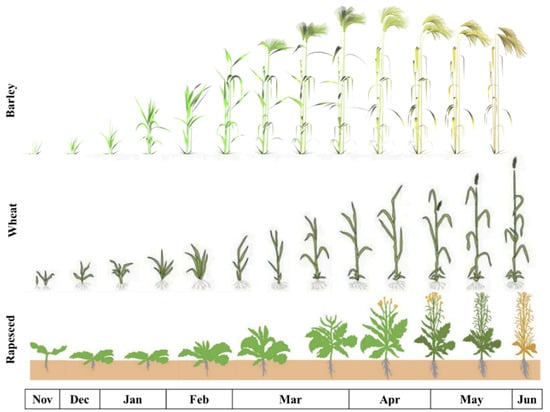
Figure 1. The growth stages of winter barley, winter wheat and winter rapeseed from late November to June [33,34,35].

3. Research Objectives

To identify and classify winter varieties of barley, wheat and rapeseed using time-series EO data and phenological studies in this research, there were five main objectives as follows:

(1)

Improve the accuracy of winter crop mapping by integrating SAR with multispectral image products. This can reduce the impact of poor-quality optical imaging acquired on cloudy days and extend the application to data acquired at different dates and times. Furthermore, it enhances EO methods by potentially identifying multiple crop types with similar optical characteristics.

(2)

Understand the growing seasons for these three winter crop types. The first step was to acquire suitable satellite imagery during the growing seasons of the three winter crops to reduce the likelihood of misclassification as spring or summer crops.

(3)

Conduct a phenological analysis of the three crop types to understand the state of the plants with various spectral indices, multi-band images, and backscattered VH (referring to vertical transmission and horizonal receipt) and VV (vertical transmission and receipt) polarisations. This analysis provides the sensitivities of the three different winter crops to the spectral indices and backscattered amplitude values via a series of given weighted inputs for integration into the final ML models.

(4)

Develop an unsupervised ML method with temporal data analysis for winter crop mapping. A supervised ML method cannot be developed without labelled ground truth. Unsupervised ML reduces the time and labour required to generate such data and, in addition, can be undertaken in areas where there is zero or limited ground truth available.

(5)

Compare and analyse the multiple, integrated results from the multispectral and SAR image products, as well as the initial crop map generated from the NDVIs and the supervised crop classifications from the Rural Payments Agency (RPA), UK [36], to form an integrated set of input variables (from Sentinel-1 and -2). It is then possible to identify the best classification results for the unsupervised ML model for winter crop type mapping.

4. Methodology

4.1. Study Area

East Anglia is located in the east of England, UK, and it consists of the counties of Norfolk, Suffolk, Cambridgeshire and Essex. It grows almost one-third of the UK’s crops, and it is considered Britain’s “breadbasket”. Compared to other regions in Britain, this region has relatively low rainfall and high temperatures, making it suitable for agriculture. Thus, Norfolk, is one of the counties in East Anglia where over 75% of the land is used for arable farming [37]. A 3 km × 3 km study area of Norfolk’s prime agricultural land was selected for this study (Figure 2), from longitude 6°47′4.618″ to 6°48′41.636″ and latitude 46°31′2.547″ to 46°32′9.297″. The main winter crops grown in Norfolk are barley, wheat and rapeseed. The other winter crops, such as oats and rye, are grown but on a smaller scale and are, therefore, not the focus of this study. The ground truth data for these winter crops were collected during field investigations across Norfolk by the RPA (Figure 2b) between June and August 2020 at 28 ground truth data location points. These sampled locations cover areas of 1.38 ${\mathrm{k}\mathrm{m}}^2$ for winter barley (13 ground truth points), 1.2 ${\mathrm{k}\mathrm{m}}^2$ for winter wheat (10 ground truth points) and 0.56 ${\mathrm{k}\mathrm{m}}^2$ for winter rapeseed (5 ground truth points). Polygons were generated for the ground truth points of the winter crops according to farm field boundaries identified using Sentinel-2 multispectral images. The ground truth polygons were divided into pixels, including 383 pixels for winter barley, 332 pixels for winter wheat and 156 pixels for winter rapeseed.

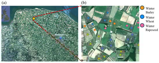
Figure 2. (a) Location of Norfolk in the UK, using a Google Earth image (inset), and a Sentinel-2 image map of Norfolk, UK, with the yellow square showing the study area; (b) detailed image of the study area and ground truth point locations for winter barley (orange), wheat (blue) and rapeseed (lilac) from RPA, UK.

4.2. General Workflow

This work required time-series images from the EO satellites Sentinel-1 and -2, as shown in the workflow. Sentinel-1 image products were registered to Sentinel-2 image products with UTM/WGS84 and both image products were resampled to the same pixel size. The values for the NDVI, Soil-Adjusted Vegetation Index (SAVI), Normalised Difference Water Index (NDWI), NDMI, EVI, VH, VV, and VH/VV were all extracted from each pixel in Stage A. In stage B, the proximity between each pixel was calculated with the Fast DTW; thus, eight proximity matrices were generated. Pixels were classified by the HC with the eight proximity matrices, and the results were georeferenced and saved as eight geoTiff files during the first stage. The eight geoTiff files were validated with the ground truth from the RPA, UK, to produce the sensitivities of the values of the NDVI, SAVI, EVI, NDWI, NDMI, VH, VV and VH/VV. In stage C, the sensitivity of each value became its given weight for each normalised proximity matrix. The normalised proximity matrices with their given weights became the final input of the HC ML models to generate the final integration results in the second stage (Figure 3).

Figure 3. The flowchart and workflow of this research.

4.3. Satellite Image Data

This research utilised Sentinel-1 SAR and multispectral (optical) image products acquired over Norfolk between November 2019 and June 2020 using data downloaded from the Alaska Satellite Facility [38] and Copernicus Open Access Hub [39].

Sentinel-1 Level-1 Interferometric Wide (IW) Ground Range Detected (GRD) image products, which are multi-looked with a 12-day revisit period and collected at dual polarisations (VH and VV backscattering measurements) are used here. These products have been projected to ground range using an Earth ellipsoid model. The spatial resolution of the GRD products is 20.4 m in the range and 22.5 m in the azimuth directions, and these image products have been resampled to provide a 10 × 10 m pixel.

Sentinel-2 Level-2A multispectral image data were collected during a 5-day repeat cycle, with 13 spectral bands spanning the coastal aerosol, visible, Near Infra-Red (NIR), water vapor and Short-Wave Infra-Red (SWIR) spectral regions, with a 60 m, 10 m and 20 m Ground Sampling Distance (GSD). Since the optical spectrum cannot penetrate through cloud cover, to avoid low-quality multispectral imagery, only images with an estimated cloud cover of less than 10% were used.

4.4. Image Data Pre-Processing to Produce Key Indices

All Sentinel image products were geo-referenced to a common WGS84 datum and UTM N31 projection, and we resampled them using bilinear interpolation to a pixel size of 60 × 60 m. A series of image spectral indices were calculated from the Sentinel-2 data using the formulas set out in Table 1 (using the spectral bands listed in Table 1). Sentinel-1 images of the backscattered amplitude values representing VH, VV and the ratio of VH/VV were also selected and calculated for use in our method.

Table 1. Generic formulae of the multispectral indices used in this method. L refers to a value representing the canopy background adjustment factor (0.5 being a general value found to minimise soil brightness variations).

Spectral Index	Formula
NDVI	(NIR − Red)/NIR + Red) [40]
SAVI	(1 + L) × (NIR − Red)/(NIR + Red + L); where L = 0.5 [41]
EVI	2.5 × (NIR − Red)/(NIR + 6 × Red − 7.5 × Blue + 1) [42]
NDMI	(NIR − SWIR)/(NIR + SWIR) [43]
NDWI	(NIR − Green)/(NIR + Green) [44]

4.5. Combined Fast Dynamic Time Warping and Hierarchical Clustering (FastDTW-HC)

This research developed a ML model by combining the following two mathematical methods: Fast DTW and HC. The procedures in the workflow were constructed for EO time-series data applications specific to crop classification.

FastDTW-HC consists of the following two sequentially applied processing methods: 1. proximity calculations using FastDTW and 2. Hierarchical Clustering (HC). Fast DTW is described in Section 4.5.1 and is the method utilised to produce proximity matrices for each variable, and these matrices form the inputs to the HC Machine Learning (ML) model. HC is described in Section 4.5.2, and involves the grouping of similar pixels according to the values in the proximity matrices of each variable and the pixels with “cluster numbers” are georeferenced and saved as a GeoTiff file.

Following the general workflow in Figure 3, FastDTW-HC for crop classification combines these methods in two stages. The first stage involves the generation of proximity matrices for eight initial HC ML models, which leads to a set of eight initial results, one from each index (NDVI, SAVI, EVI, NDMI, NDWI, VH, VV and VH/VV, as listed in Table 2), which are aimed at calculating the sensitivity (i.e., recall) of each index for barley, wheat and rapeseed with Equation (1). To understand the sensitivities of the eight index values, the eight initial results are validated against the RPA ground truth. The sensitivity of each index to barley, wheat and rapeseed is transformed to derive weights for the input proximity matrices of each index, which are used in the second stage. In the second stage, the proximity matrices of each index are calculated by FastDTW, weighted and normalised before being input in the HC ML model. The input normalised proximity matrices are defined with different index combinations, as shown in Table 2.

Table 2. The five combinations of indices (multispectral indices and SAR amplitude images) tested with the FastDTW-HC ML model.

R1	NDVI + SAVI + EVI + NDMI
R2	NDVI + SAVI + EVI + NDMI + NDWI
R3	NDVI + VH + VV + VH/VV
R4	NDVI + SAVI + EVI + NDMI + VH + VV + VH/VV
R5	NDVI + SAVI + EVI + NDMI + NDWI + VH + VV + VH/VV

This second stage works with the five different combinations of the index (referred to as R1 to R5, as shown in Table 2) and their normalised proximity matrices: four normalised proximity matrices (NDVI, SAVI, EVI and NDMI) for the HC ML model of R1; five normalised proximity matrices (NDVI, SAVI, EVI, NDMI and NDWI) for the HC ML model of R2; four normalised proximity matrices (NDVI, VH, VV and VH/VV) for the HC ML model of R3; seven normalised proximity matrices (NDVI, SAVI, EVI, NDMI, VH, VV and VH/VV) for the HC ML model of R4; and eight normalised proximity matrices (NDVI, SAVI, EVI, NDMI, NDWI, VH, VV and VH/VV) for the HC ML model of R5.

$$\mathrm{R}\mathrm{e}\mathrm{c}\mathrm{a}\mathrm{l}\mathrm{l}/\mathrm{S}\mathrm{e}\mathrm{n}\mathrm{s}\mathrm{i}\mathrm{t}\mathrm{i}\mathrm{v}\mathrm{i}\mathrm{t}\mathrm{y}={\displaystyle \frac{\mathrm{T}\mathrm{P}}{\mathrm{T}\mathrm{P}+\mathrm{F}\mathrm{N}}}$$

(1)

4.5.1. Calculating Proximity with Fast DTW

The DTW is a robust proximity calculation method of similarities, which reduces the influence of irregular sampling in time-series caused by satellite imaging that is often affected by weather and clouds [20], and it was utilised to generate the proximity matrices in this research. The general concept of the DTW is shown in Figure 4. Unlike the traditional Euclidean method, which calculates the similarities (distances) of pixels X and Y at the same point in time, in the two time-series, the DTW performs the dynamic similarity calculation within the time-series at multiple time points.

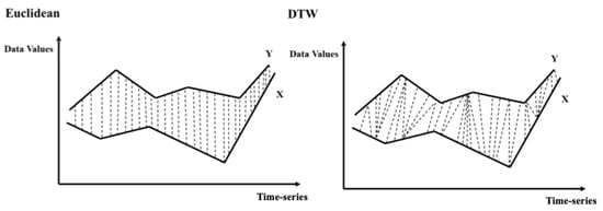
Figure 4. The general concepts of the Euclidean and DTW similarity (distance) calculations between pixels X and Y in two time-series.

Mathematically, it does this by quantifying the similarity between two time-series datasets to find the warping alignment in their temporal patterns, calculated as the minimum of the cumulative similarity distances of the pixels in two time-series, as illustrated in Figure 5. In this research, the similarity between pixels in two time-series was calculated from the matrix constructed from the two sets of index values on a pixel-by-pixel basis. The time-series of index values for two pixels, X and Y, were calculated using Equations (2) and (3), with the lengths of time-series n and m, as follows:

X = x1, x2, …, xi, …, xn

(2)

Y = y1, y2, …, yj, …, ym

(3)

where x and y are the individual index values for a pixel acquired at a specific time in the time-series; thus, they form an n-by-m matrix from the similarity of the pixels in the X and Y time-series to generate the warping elements, ${\mathrm{w}}_{\mathrm{k}}={(\mathrm{i},\mathrm{j})}_{\mathrm{k}}$, which are utilised to form a single or multiple warping paths, as shown in Figure 5. Several “warping paths” can be found between these two time-series, with a total of K warping elements, as follows:

$$\mathrm{D}\mathrm{T}\mathrm{W}(\mathrm{X},\mathrm{Y})=\mathrm{m}\mathrm{i}\mathrm{n}\left\{\sqrt{{\sum }_{\mathrm{k}=1}^{\mathrm{K}}{\mathrm{w}}_{\mathrm{k}}}\right\}$$

(4)

where K is the total number of warping elements, and k is the number of individual warping elements.

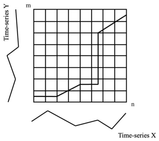
Figure 5. Illustration of a “warp path” between the index values of two pixels in two time-series datasets, X and Y, in an n-by-m matrix of time points, where the “warp path” represents the similarity between the index values of two pixels in time-series n and m.

Deriving the optimal warping alignment for the similarity calculations from thousands of pixels in time-series datasets can be highly computationally expensive, requiring very large amounts of RAM and long running times. To overcome these issues, the Fast DTW method is applied, which involves the following three key steps: coarsening, projection and refinement. 1. Coarsening progressively up-samples each time-series to produce multiple matrices with a decreasing number of n and m elements by averaging adjacent pairs of points, as illustrated in Figure 6. 2. In the projection stage, the optimal warping alignment for each case is found at the (lowest) poorest “resolution” and is gradually projected to the highest resolution. 3. In the Refinement stage, whilst the optimal warping alignment is projected from the lowest resolution to the highest, it is refined with local adjustments among the neighbourhood of values around the projected path. Fast DTW involves a multi-level approach via these three stages, which reduces the processing demands by downsizing the distance matrix in the DTW algorithms. In the case of the DTW, the optimal warping alignment is calculated from all warping elements generated from every element in the n-by-m matrix, whereas Fast DTW generates the optimal warping alignment at levels of increasing complexity and processes only the relevant neighbouring elements of any projected optimal warp alignment from the previous lower resolution level matrix, as shown in Figure 6 [45]. After the optimal warping alignment between each index of each pixel is generated, the optimal warping alignments of each index of pixels are saved as a proximity matrix.

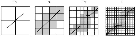
Figure 6. An example of the Fast DTW process on an optimal warping alignment with local neighbourhood adjustments from a 1/8 resolution to the original resolution.

4.5.2. Hierarchical Clustering

The proximity matrices of each index generated from the Fast DTW form the input variables of the HC ML models. This research applied the HC ML methods to generate the eight initial results using the winter crop maps from each spectral index and the backscattered amplitude values. From the eight FastDTW-HC models, the sensitivity (i.e., recall) of each index for barley, wheat and rapeseed was calculated, and the final five integration results produced five FastDTW-HC models with the sensitivity of each index.

Utilising the proximity matrices, image pixels were clustered by the HC agglomerative method, which is a “bottom-up” approach, starting with a single pixel as a cluster and progressively merging single clusters into larger clusters until all pixels are classified into the same cluster (unless certain termination conditions are set), as illustrated in Figure 7. HC classifies those pixels by calculating the similarity distances between the proximity matrices using the complete-link (also called the diameter) algorithm in Equation (5) [46]. This algorithm calculates the similarity distance between two clusters with the maximum of all pairwise distances between any members of one cluster to any members of the other cluster [47].

$$max\left\{d\left(a,b\right):a\in A,b\in B\right\}$$

(5)

where A and B represent two respective clusters; a and b represent one of the patterns in each cluster; and d represents the distance between a and b.

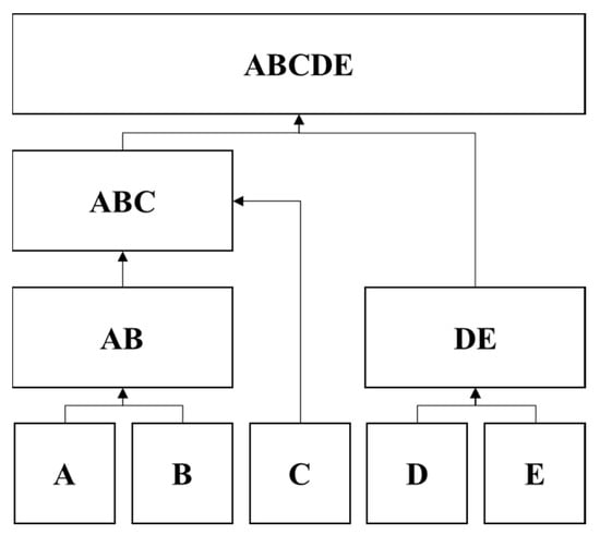
Figure 7. A graphical illustration of the hierarchical clustering concept. Five individual (conceptual) clusters (A, B, C, D and E) are clustered according to their similarity (i.e., distance) values. Clusters A and B and clusters D and E then form new clusters of AB and DE, whilst C remains alone. Similarities among AB, DE and the individual cluster C, are then used to form the second layer. Since C is more similar to AB, a new ABC cluster is formed whilst DE remains. The final layer gathers all remaining clusters into one large cluster, ABCDE, and the dendrogram of A, B, C, D and E is formed [48].

4.6. Validation Against RPA In Situ Data

The final FastDTW-HC integration results (R1 to R5) were validated against the in situ “ground truth” pixels in the study area. These results included 383 pixels of barley, 332 pixels of wheat and 156 pixels of rapeseed. The recall, precision, accuracy and F1 scores, as well as kappa coefficients, from the final integration results were calculated using Equations (1) and (6) to (11), which are provided in Table 3.

$$\mathrm{P}\mathrm{r}\mathrm{e}\mathrm{c}\mathrm{i}\mathrm{s}\mathrm{i}\mathrm{o}\mathrm{n}={\displaystyle \frac{\mathrm{T}\mathrm{P}}{\mathrm{T}\mathrm{P}+\mathrm{F}\mathrm{P}}}$$

(6)

Table 3. Kappa coefficient calculations for an example involving three elements judged by Rater1 and Rater2.

	Rater2
Rater1		A	B	C	Totals
	A	AA	AB	AC	Rater1A
	B	BA	BB	BC	Rater1B
	C	CA	CB	CC	Rater1C
	Totals	Rater2A	Rater2B	Rater2C	ABC

$$\mathrm{A}\mathrm{c}\mathrm{c}\mathrm{u}\mathrm{r}\mathrm{a}\mathrm{c}\mathrm{y}={\displaystyle \frac{\mathrm{T}\mathrm{N}+\mathrm{T}\mathrm{P}}{\mathrm{T}\mathrm{N}+\mathrm{F}\mathrm{P}+\mathrm{T}\mathrm{P}+\mathrm{F}\mathrm{N}}}$$

(7)

$$\mathrm{F}1\mathrm{S}\mathrm{c}\mathrm{o}\mathrm{r}\mathrm{e}={\displaystyle \frac{2}{\frac{1}{\mathrm{P}\mathrm{r}\mathrm{e}\mathrm{c}\mathrm{i}\mathrm{s}\mathrm{i}\mathrm{o}\mathrm{n}}+\frac{1}{\mathrm{R}\mathrm{e}\mathrm{c}\mathrm{a}\mathrm{l}\mathrm{l}}}}={\displaystyle \frac{2\ast \mathrm{P}\mathrm{r}\mathrm{e}\mathrm{c}\mathrm{i}\mathrm{s}\mathrm{i}\mathrm{o}\mathrm{n}\ast \mathrm{R}\mathrm{e}\mathrm{c}\mathrm{a}\mathrm{l}\mathrm{l}}{\mathrm{P}\mathrm{r}\mathrm{e}\mathrm{c}\mathrm{i}\mathrm{s}\mathrm{i}\mathrm{o}\mathrm{n}+\mathrm{R}\mathrm{e}\mathrm{c}\mathrm{a}\mathrm{l}\mathrm{l}}}$$

(8)

$$P_o=(AA+BB+CC)/ABC$$

(9)

$$P_e={\displaystyle \frac{Rater1A\ast Rater2A}{{ABC}^2}}+{\displaystyle \frac{Rater1B\ast Rater2B}{{ABC}^2}}+{\displaystyle \frac{Rater1C\ast Rater2C}{{ABC}^2}}$$

(10)

$$\mathrm{Kappa}=(P_o-P_e)/(1-P_e)$$

(11)

5. Crop Classification Results

5.1. Winter Crop Maps

Aiming to reduce the impact of any low-quality, slightly cloudy Sentinel-2 images that may be present, an unsupervised classification using NDVI, VH, VV and VH/VV images was generated and compared to the RPA supervised classification (Figure 8a). Comparing R3 with the NDVI only (Figure 8c and Figure 8b, respectively), the identification of winter wheat is improved by the inclusion of the backscattered amplitude values of VV, VH and VH/VV but is relatively unreliable for other crops and produces a kappa coefficient of only 0.17, as well as overall accuracies, precisions and F1 scores, as shown in Table 4.

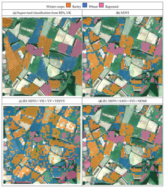
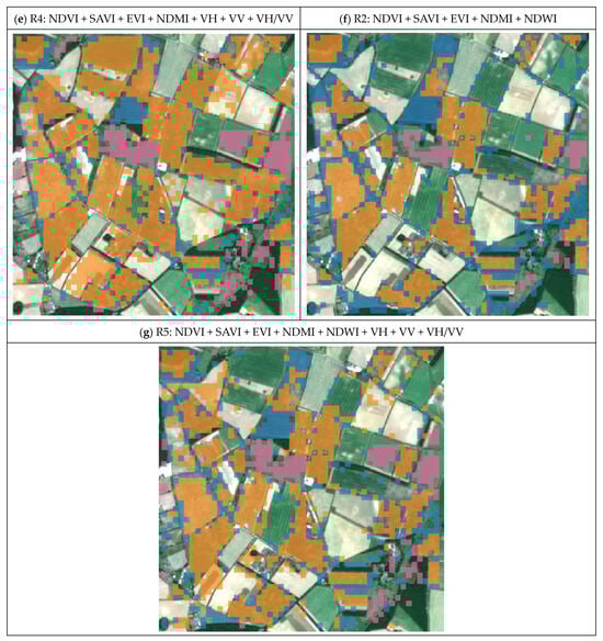
Figure 8. (a) Supervised classification results on winter crops produced by the RPA (RPA, 2021); (b) initial result with the NDVI and the final integration results with R1 to R5 (c–g). Orange represents barley, blue represents wheat and lilac represents rapeseed.

Table 4. Statistical analysis of the classification results with the NDVI only and with R1 to R5.

NDVI Only
	Recall	Precision	Accuracy	F1 Score	Kappa
Barley	91%	64%	74%	0.75	0.45
Wheat	20%	65%	66%	0.31
Rapeseed	69%	92%	93%	0.79
R3: NDVI + VH + VV + VH/VV
Barley	33%	49%	55%	0.39	0.17
Wheat	53%	44%	56%	0.48
Rapeseed	45%	100%	90%	0.62
R1: NDVI + SAVI + EVI + NDMI
Barley	81%	72%	78%	0.76	0.59
Wheat	28%	68%	68%	0.4
Rapeseed	77%	98%	96%	0.86
R4: NDVI + SAVI + EVI + NDMI + VH + VV + VH/VV
Barley	85%	58%	66%	0.69	0.35
Wheat	17%	55%	63%	0.26
Rapeseed	62%	98%	93%	0.76
R2: NDVI + SAVI + EVI + NDMI + NDWI
Barley	81%	66%	73%	0.73	0.35
Wheat	32%	57%	65%	0.41
Rapeseed	31%	100%	88%	0.47
R5: NDVI + SAVI + EVI + NDMI + NDWI + VH + VV + VH/VV
Barley	86%	66%	76%	0.75	0.52
Wheat	28%	76%	69%	0.41
Rapeseed	61%	100%	93%	0.76

Identifying the most suitable combination of variables for the unsupervised model requires two series of final integration results from the various input variables. These two series of integration results include those generated only from spectral indices (R1 and R2) and those which also include backscattered amplitude values (R3, R4 and R5), as illustrated in Figure 8.

Using the statistical analysis in Table 4, R1 in Figure 8g provides the best and most reliable result with a kappa coefficient of 0.59 and accuracies of 78% for barley, 68% for wheat and 96% for rapeseed. As the second most reliable result, R5 had a kappa coefficient of 0.52 and accuracies of 76% for barley, 69% for wheat and 93% for rapeseed. The main advantages of R5 over R1 are the precision value of wheat, hence the more precise mapping of wheat, at 76%, and the increase in the identification of barley to 86% with the recall, by including the NDWI and backscattered amplitude values. Evaluating the influence of the amplitude values in R1 and R4, the identification of barley improved, with the recall increasing from 81% to 85%, an increase of 4%. The overall influence of the NDWI on winter crop mapping can be observed by comparing the differences between R1 and R2. R1 lacks the ability to identify wheat, with a recall of only 28%; however, by including the NDWI, the identification of wheat can be improved.

Comparing the ground truth in Figure 2b and the RPA’s supervised classification in Figure 8a with the unsupervised classifications R1 and R5, it is clear that the supervised classification, which uses ground truth, produced the most accurate results, with accuracies of 84% for barley, 76% for wheat and 94% for rapeseed. The overall identification of winter crops, as well as the classification of barley and wheat, was more accurate using a supervised approach with reliable ground truth than with R1 and R5. However, R1 and R5 approached similar levels of accuracy as the RPA supervised classification and demonstrated improved accuracy and precision in the classification of winter crops compared to previous research studies without the use of ground truth data. This unsupervised approach reduces the time and labour costs and highlights what can be achieved when ground truth data are not available. On occasion, R1 and R5 misclassified some hedgerows as wheat, as well as some “set-aside” areas in barley fields as wheat. Some of these may be misclassifications, but when the results are compared with Sentinel-2 imagery acquired in May 2020, it appears that some hedgerows and set-aside areas around the margins of the barley fields are, indeed, growing winter wheat. This indicates that our proposed unsupervised classification method can function well in a mixed-crop environment, on local and regional scales, but we suggest that the best validation approach should include visual inspection of the multispectral images, as well as field investigation.

The R1 to R5 and NDVI results, as shown in Figure 8, which references the field investigation by the RPA, indicate that some spring barley fields are classified as barley and/or wheat because of the similar phenology of their spring and winter varieties. The best results were obtained using R1 and R5.

Overall, the integration of multispectral and SAR imagery improves the identification of winter varieties of barley and wheat. Furthermore, with the combination of spectral indices and backscattered amplitude values, our R1 and R5 unsupervised ML methods provided the best results for the winter food crop mapping and are suitable for mixed crop farming.

5.2. Monitoring of Winter Crop Phenology

Using one of the most robust results with multispectral and SAR images, R5, we investigated the patterns of winter crop phenology, as shown in Figure 9, where the months of the growing season are shown on the X-axes of the plots, orange lines represent barley, blue lines wheat and lilac lines rapeseed. In Figure 9a, the NDVI values of the three winter crops throughout the growing season are shown; it can be seen that barley and wheat are very similar and this, on occasion, led to misclassifications. Since the pattern of the NDVI values for rapeseed was slightly different to those of barley and wheat, only rapeseed was effectively recognised with this unsupervised classification.

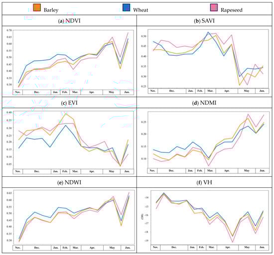
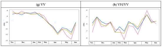
Figure 9. Spectral index and amplitude values throughout the growing season for winter varieties of barley (orange), wheat (blue) and rapeseed (lilac).

Because of the similarities between the winter crop NDVI patterns throughout the growing season, additional multispectral indices and SAR backscattered amplitude values were used to improve the unsupervised classification. By including the SAVI, EVI and NDMI, the identification of wheat and the precision of barley and rapeseed mapping improved. The kappa coefficient increased, and this demonstrates that the integration of additional variables provides a more reliable result than the NDVI alone. The differences in the SAVI, EVI and NDMI patterns among the three types of winter crops explain the improvement with the unsupervised classification. Compared to the NDVI, the SAVI, EVI and NDMI trends were very different across the three crop types. Due to the flowering season and structural changes in the leaves and plants (see Figure 1), we observed a large drop in the EVI value in April and in the SAVI value in May, and these make significant contributions to the classification. In Figure 9e, the pattern of the NDWI values is similar to that of the NDVI, and the NDWI patterns of barley and wheat also have high similarity, which reduces the reliability of the wheat identification compared to the results from the NDVI only and R2, as shown in Figure 8. If backscattered amplitude values are included, the identification of winter crops improve, especially wheat with R1 and R5 and barley with R4 and R5. Although the backscattered amplitude values are relatively low for the winter crops, the patterns of the VH, VV and VH/VV values allow for the identification of the three crop types with dynamic structural changes, as illustrated in Figure 1, which advances our approach to the unsupervised classification of crops. The significant contribution of the VV is highlighted by the very similar patterns among the three winter crops throughout the year, as shown in Figure 9g. Furthermore, the high sensitivity of the winter crops to VV is recognised in the initial results, which are very similar to the contributions made by the SAVI and EVI.

As demonstrated by the temporal analysis and the initial results of the multispectral indices and backscattered amplitude values, the NDVI made the greatest contribution, whilst the SAVI, NDMI, EVI, VH and VV also made important contributions to the unsupervised classification model for the three winter crops.

6. Discussion

This research demonstrates that classification using only spectral indices from multispectral image products provide acceptable results, but by integrating these with SAR image products, the precision and accuracy of individual winter crop classifications can significantly improve, even though the contributions of the backscattered measurements are smaller than the spectral indices, as shown in Table 5. Low contributions from the backscattered measurements for winter crops can be seen in research using the DTW and Sentinel-1 and TerraSAR-X for complex farming classifications, where the analysis of the accuracies for winter crops indicates they were relatively low [49].

Table 5. The sensitivity (i.e., recall) of the variables (spectral indices and backscattered amplitude values) for barley, wheat and rapeseed in the FastDTW-HC models.

	Variable	NDVI	SAVI	EVI	NDMI	NDWI	VH	VV	VH/VV
Sensitivity
Barley		91%	46%	43%	95%	81%	81%	81%	49%
Wheat		20%	20%	45%	20%	19%	19%	0%	9%
Rapeseed		69%	96%	50%	26%	33%	44%	67%	60%

The sensitivities of the spectral indices and backscattered amplitude values in classifying winter crops were calculated from the eight initial results using the FastDTW-HC models. In general, for recognising winter crops, the NDVI outperformed all of the other variables, but it had a relatively low sensitivity to rapeseed. The SAVI showed higher sensitivities to rapeseed, at 96%, but low sensitivities to barley, as shown in Table 5.

The NDMI had slightly higher sensitivity to barley and the same sensitivity to wheat compared to the NDVI. The spectral indices and VH backscattered measurement shared similar sensitivities, at around 20% for wheat, which represent minor contributions of each variable in R5. The VV backscattered measurement and VH/VV ratio, on the other hand, made significant contributions on the extraction of rapeseed compared to the other variables.

Statistical analysis of the RPA’s supervised classification shows accuracies of 84% for barley, 76% for wheat and 94% for rapeseed. The FastDTW-HC unsupervised model used here exhibited accuracies with R4 of 78% for barley, 68% for wheat and 96% for rapeseed and with R5 of 76% for barley, 69% for wheat and 93% for rapeseed. Comparing the best performing outcomes of the unsupervised classification (R1 and R5) to the RPA’s supervised classification in 2020, it can be observed that the supervised classification results are better across this same study area. However, supervised classification relies on ground truth training samples from the study area and during the same time period.

The unsupervised learning methods (K-means and Gaussian mixture models (GMM)) used in previous research studies are only suitable for large farming areas growing two types of crops and require optimised sowing and harvest times for more accurate classifications [50]. Ma et al. (2020) developed a Principal Components Isometric Binning (PCIB) unsupervised classification method, but this was only tested with two crop types, rice and maize, from 2010 to 2017, and when applied on multiple crop types in 2018 resulted in many misclassifications, especially for set-asides and hedgerows, which were recognised as maize [51]. The inaccurate classifications influenced by hedgerows, set-asides and mixed-crop areas can influence future predictions of crop yields and biomass based on the digital crop maps.

According to the unsupervised classification with FastDTW-HC in this research and the supervised classification by the RPA, some hedgerows and set-asides around the field margins were misclassified as either wheat or barley in both winter crop maps. This situation can also be found in previous research studies on crop classification using supervised and unsupervised ML and DL approaches with satellite or aerial imagery [52,53,54,55]. However, by observing the crop patterns in the Sentinel-2 images, it can be seen that some fields are “mix-cropped”, which leads to some errors in the validation of the results, requiring further field-based investigations. This demonstrates that the FastDTW-HC model is capable of mapping mixed winter crops. The validation process, forming part of this research, is conducted on a pixel-by-pixel basis, offering more detail, accuracy and precision due to the complexity of farming types compared to previous research studies that classified and validated the results by field. This leads to a moderate kappa coefficient. In future research, when this method is applied on a regional scale, crops will be identified in 3 km by 3 km open windows and a more robust validation will be provided.

This winter crop mapping method involves the selection of satellite imaging dates that follow the growing season of winter crops to avoid misclassifications caused by summer crops. However, even in the best results, with R1 and R5, some spring barley and winter wheat fields were identified as winter barley fields because of their similar phenological stages. To resolve this issue, multi-sensor products are suggested to be used in future research to provide more detailed time-series data for precise temporal analysis during particular phenological stages.

7. Conclusions

This research identifies three winter crop types—barley, wheat and rapeseed—from a temporal analysis of a series of spectral indices. When analysing the sensitivities of each variable (Figure 8), the NDVI (Figure 8b) was shown to be the most important spectral index for recognising the three winter crop types. Thus, this research was developed from the baseline provided by the initial results in Figure 8b and evaluated other combinations of image variables and other spectral indices and backscattered amplitude values to improve the unsupervised classification of winter crop types, as illustrated in Figure 8. The RPA’s supervised classification, shown in Figure 8a, using reliable ground truth data produced the most accurate results, and the identifications of barley and wheat were more precise than with R1 and R5. However, R1 and R5 reached similar levels of accuracy as the RPA’s supervised classification and showed improved results compared to supervised classifications in previous research studies.

This work developed an unsupervised classification method for winter crop mapping generated by a reliable FastDTW-HC process with clear procedures that do not rely on ground truth data. The FastDTW-HC model extracted and analysed the main winter crops grown across Norfolk, UK, which can be directly applied in regions growing winter barley, wheat and rapeseed. This method can be utilised on multiple crop types once the phenological stages of the biology are understood using earth observation techniques. The integrated multispectral and SAR images are used in the time-series to advance the crop type mapping, and the following are the seven main outcomes of this work:

(1)

The analysis of the integrated results determined the following most suitable combination of spectral indices and backscattered amplitude values for winter crop mapping using the FastDTW-HC model: NDVI, SAVI, EVI, NDMI, NDWI, VH, VV and VH/VV.

(2)

The best performance results were with R1 and R5, which had moderate kappa coefficients of 0.59 and 0.52 and acceptable accuracies of 78% and 76% for barley, 68% and 69% for wheat and 96% and 93% for rapeseed. This means the model is reliable and the combinations of spectral indices with R1 and R5 are suggested to be used in future research. Comparing R1 and R5, R5 including backscattered measurements can provide better precision in the identification of winter wheat.

(3)

Temporal analysis of the multispectral indices and backscattered SAR amplitude values can enhance the understanding of seasonal growth patterns of winter varieties of barley, wheat and rapeseed. By understanding the phenological stages of crops with EO data, farmers can better schedule periods of irrigation, pesticide application and harvest.

(4)

The sensitivities of each spectral index and backscattered amplitude values were analysed for the winter crops throughout the growing season, providing crop maps and temporal analysis.

(5)

The unsupervised classifications, R1 and R5 from the FastDTW-HC model, had similar levels of accuracy as that of the supervised classification published by the RPA. The development of this model can benefit policymakers interested in crop land management and food sustainability. In addition, food security issues in regions for which no field ground truth data are available can be improved by utilising the EO method in this study to produce accurate crop maps for crop growing plans and potential food distribution.

(6)

Observations of arable fields using optical satellite images reveal that the FastDTW-HC model developed in this research is suitable for complex farming areas, including those where mixed crops and set-asides are used.

(7)

Using the methods developed in this work and previous research, the analysis of spectral indices throughout growth cycles can aid in classifying different crop types in multiple regions under various soil and meteorological conditions.

8. Future Works

With an enhanced understanding of winter crop phenology and the high accuracy of classification results, future land management strategies can be improved. Furthermore, observations and predictions of biomass and yield across winter crops can be made more precisely with more accurate crop maps. By monitoring biomass and yields, winter crop planting strategies can be improved with crop rotations and mixed crops to maintain soil health and ensure maximum yields.

The next research steps will be to monitor the biomass and yields, and the proposed FastDTW-HC model will be applied on a regional agricultural scale for winter crop mapping. Maps of winter barley, wheat and rapeseed between 2018 and 2023 across Norfolk will be of interest as a next step. Combining winter crop maps with meteorological data and field investigations can further improve this multivariate statistical method to provide better predictions of yield and biomass.

References

- Allen, M.R.; Dube, O.P.; Sloecki, W.; Aragón-Durand, F.; Cramer, W.; Humphreys, S.; Kainuma, M.; Kala, J.; Mahowald, N.; Mulugetta, Y.; et al. 2018: Framing and Context. In Global Warming of 1.5 °C. An IPCC Special Report on the Impacts of Global Warming of 1.5 °C Above Pre-Industrial Levels and Related Global Greenhouse Gas Emission Pathways, in the Context of Strengthening the Global Response to the Threat of Climate Change, Sustainable Development, and Efforts to Eradicate Poverty; Cambridge University Press: Cambridge, UK; New York, NY, USA, 2022; pp. 49–92. [Google Scholar] [CrossRef]
- Wheeler, T.; von Braun, J. Climate Change Impacts on Global Food Security. Science 2013, 341, 508–513. [Google Scholar] [CrossRef] [PubMed]
- Ahmed, Z.; Nalley, L.; Brye, K.; Green, V.S.; Popp, M.; Shew, A.M.; Connor, L. Winter-time cover crop identification: A remote sensing-based methodological framework for new and rapid data generation. Int. J. Appl. Earth Obs. Geoinf. 2023, 125, 103564. [Google Scholar] [CrossRef]
- Wang, L.; Dong, Q.; Yang, L.; Gao, J.; Liu, J. Crop Classification Based on a Novel Feature Filtering and Enhancement Method. Remote Sens. 2019, 11, 455. [Google Scholar] [CrossRef]
- KC, K.; Zhao, K.; Romanko, M.; Khanal, S. Assessment of the Spatial and Temporal Patterns of Cover Crops Using Remote Sensing. Remote Sens. 2021, 13, 2689. [Google Scholar] [CrossRef]
- You, N.; Dong, J. Examining earliest identifiable timing of crops using all available Sentinel 1/2 imagery and Google Earth Engine. ISPRS J. Photogramm. Remote Sens. 2020, 161, 109–123. [Google Scholar] [CrossRef]
- Barriere, V.; Claverie, M.; Schneider, M.; Lemoine, G.; d’Andrimont, R. Boosting crop classification by hierarchically fusing satellite, rotational, and contextual data. Remote Sens. Environ. 2024, 305, 114110. [Google Scholar] [CrossRef]
- Blaes, X.; Vanhalle, L.; Defourny, P. Efficiency of crop identification based on optical and SAR image time series. Remote Sens. Environ. 2005, 96, 352–365. [Google Scholar] [CrossRef]
- McNairn, H.; Champagne, C.; Shang, J.; Holmstrom, D.A.; Reichert, G. Integration of optical and Synthetic Aperture Radar (SAR) imagery for delivering operational annual crop inventories. Isprs. J. Photogramm. Remote Sens. 2009, 64, 434–449. [Google Scholar] [CrossRef]
- Ianninia, L.; Molijn, R.A.; Hanssen, R.F. Integration of multispectral and C-band SAR data for crop classification. In Proceedings of the SPIE, Dresden, Germany, 16 October 2013. [Google Scholar] [CrossRef]
- Bargiel, D. A new method for crop classification combining time series of radar images and crop phenology information. Remote Sens. Environ. 2017, 198, 369–383. [Google Scholar] [CrossRef]
- Van Tricht, K.; Gobin, A.; Gilliams, S.; Piccard, I. Synergistic use of radar Sentinel-1 and optical sentinel-2 imagery for crop mapping: A case study for Belgium. Remote Sens. 2018, 10, 1642. [Google Scholar] [CrossRef]
- Robertson, L.D.; Davidson, A.; McNairn, H.; Hosseini, M.; Mitchell, S.; De Abelleyra, D.; Verón, S.; le Maire, G.; Plannells, M.; Valero, S.; et al. C-band synthetic aperture radar (SAR) imagery for the classification of diverse cropping systems. Int. J. Remote Sens. 2020, 41, 9628–9649. [Google Scholar] [CrossRef]
- Xun, L.; Zhang, J.; Cao, D.; Yang, S.; Yao, F. A novel cotton mapping index combining Sentinel-1 SAR and Sentinel-2 multispectral imagery. Isprs J. Photogramm. Remote Sens. 2021, 181, 148–166. [Google Scholar] [CrossRef]
- Blickensdörfer, L.; Schwieder, M.; Pflugmacher, D.; Nendel, C.; Erasmi, S.; Hostert, P. Mapping of crop types and crop sequences with combined time series of Sentinel-1, Sentinel-2 and Landsat 8 data for Germany. Remote Sens. Environ. 2022, 269, 112831. [Google Scholar] [CrossRef]
- Leite, P.B.C.; Feitosa, R.Q.; Formaggio, A.R.; da Costa, G.A.O.P.; Pakzad, K.; Sanches, I.D. Hidden Markov models for crop recognition in remote sensing image sequences. Pattern Recogn. Lett. 2011, 32, 19–26. [Google Scholar] [CrossRef]
- Siachalou, S.; Mallinis, G.; Tsakiri-Strati, M. A Hidden Markov models approach for crop classification: Linking crop phenology to time series of multi-sensor remote sensing data. Remote Sens. 2015, 7, 3633. [Google Scholar] [CrossRef]
- Lafferty, J.D.; McCallum, A.; Pereira, F. Conditionalrandom fields: Probabilistic models for segmenting and labelling sequence data. In ICML; Morgan Kaufmann: San Fran-cisco, CA, USA, 2001; pp. 282–289. [Google Scholar]
- Kenduiywo, B.; Bargiel, D.; Soergel, U. Spatial-Temporal Conditional Random Fields Crop Classification from TerraSAR-X Images. ISPRS Annals of Photogrammetry. Remote Sens. Spat. Inf. Sci. 2015, II-3/W4, 79–86. [Google Scholar] [CrossRef]
- Maus, V.; Câmara, G.; Appel, M.; Pebesma, E. dtwSat: Time-Weighted Dynamic Time Warping for Satellite Image Time Series Analysis in R. J. Stat. Softw. 2019, 88, 5. [Google Scholar] [CrossRef]
- Li, M.; Bijker, W. Vegetable classification in Indonesia using Dynamic Time Warping of Sentinel-1A dual polarization SAR time series. Int. J. Appl. Earth Obs. Geoinf. 2019, 78, 268–280. [Google Scholar] [CrossRef]
- Natteshan, N.; Kumar, N. Effective SAR image segmentation and classification of crop areas using MRG and CDNN techniques. Eur. J. Remote Sens. 2020, 53 (Suppl. S1), 126–140. [Google Scholar] [CrossRef]
- Lobert, F.; Löw, J.; Schwieder, M.; Gocht, A.; Schlund, M.; Hostert, P.; Erasmi, S. A deep learning approach for deriving winter wheat phenology from optical and SAR time series at field level. Remote Sens. Environ. 2023, 298, 113800. [Google Scholar] [CrossRef]
- Chen, Y.; Keogh, E.; Hu, B.; Begum, N.; Bagnall, A.; Mueen, A.; Batista, G. The UCR Time Series Classification Archive. 2015. Available online: www.cs.ucr.edu/~eamonn/time_series_data/ (accessed on 10 November 2024).
- Keogh, E.; Ratanamahatana, C. Exact indexing of dynamic time warping. Knowl Inf Syst 2015, 7, 358–386. [Google Scholar] [CrossRef]
- Demšar, J. Statistical comparisons of classifiers over multiple data sets. J. Mach. Learn. Res. 2006, 7, 1–30. [Google Scholar]
- Łuczak, M. Hierarchical clustering of time series data with parametric derivative dynamic time warping. Expert Syst. Appl. 2016, 62, 116–130. [Google Scholar] [CrossRef]
- AlMahamid, F.; Grolinger, K. Agglomerative Hierarchical Clustering with Dynamic Time Warping for Household Load Curve Clustering. arXiv 2022. [Google Scholar] [CrossRef]
- Marais Sicre, C.; Inglada, J.; Fieuzal, R.; Baup, F.; Valero, S.; Cros, J.; Huc, M.; Demarez, V. Early Detection of Summer Crops Using High Spatial Resolution Optical Image Time Series. Remote Sens. 2016, 8, 591. [Google Scholar] [CrossRef]
- Marszalek, M.; Lösch, M.; Körner, M.; Schmidhalter, U. Early Crop-Type Mapping Under Climate Anomalies. Environ. Sci. 2022; Preprints. [Google Scholar] [CrossRef]
- Ashourloo, D.; Nematollahi, H.; Huete, A.; Aghighi, H.; Azadbakht, M.; Shahrabi, H.S.; Goodarzdashti, S. A new phenology-based method for mapping wheat and barley using time-series of Sentinel-2 images. Remote Sens. Environ. 2022, 280, 113206. [Google Scholar] [CrossRef]
- Veloso, A.; Mermoz, S.; Bouvet, A.; Toan, T.L.; Planells, M.; Dejoux, J.; Ceschia, E. Understanding the temporal behavior of crops using Sentinel-1 and Sentinel-2-like data for agricultural applications. Remote Sens. Environ. 2017, 199, 415–426. [Google Scholar] [CrossRef]
- Kuester, T.; Spengler, D. Structural and Spectral Analysis of Cereal Canopy Reflectance and Reflectance Anisotropy. Remote Sens. 2018, 10, 1767. [Google Scholar] [CrossRef]
- Long, A. Late-Season Winter Wheat Disease and Management. Available online: https://www.beckshybrids.com/resources/croptalk-newsletter/late-season-winter-wheat-disease-and-management (accessed on 18 March 2024).
- Lidea. RAPESEED DISEASES AND PESTS ADVICE. Available online: https://lidea-seeds.com/rapeseed-diseases-and-pests-advice (accessed on 18 March 2024).
- Crop Map of England (CROME). Available online: https://www.data.gov.uk/dataset/be5d88c9-acfb-4052-bf6b-ee9a416cfe60/crop-map-of-england-crome-2020#licence-info (accessed on 9 April 2023).
- Campaign for the Farm Environment—CFE County Priorities for Norfolk. Available online: https://www.cfeonline.org.uk/archive?treeid=36011 (accessed on 5 November 2024).
- Sentinel-1—Missions—Sentinel Online—Sentinel Online. (n.d.) Available online: https://sentinel.esa.int/web/sentinel/missions/sentinel-1 (accessed on 9 April 2023).
- Sentinel-2—Missions—Sentinel Online—Sentinel Online. (n.d.) Available online: https://sentinel.esa.int/web/sentinel/missions/sentinel-2 (accessed on 9 April 2023).
- Goward, S.N.; Markham, B.; Dye, D.G.; Dulaney, W.; Yang, J. Normalized difference vegetation index measurements from the advanced very high resolution radiometer. Remote Sens. Environ. 1991, 35, 257–277. [Google Scholar] [CrossRef]
- Huete, A.R. A soil-adjusted vegetation index (SAVI). Remote Sens. Environ. 1988, 25, 295–309. [Google Scholar] [CrossRef]
- Liu, H.Q.; Huete, A. A feedback based modification of the NDVI to minimize canopy background and atmospheric noise. IEEE Trans. Geosci. Remote Sens. 1995, 33, 457–465. [Google Scholar] [CrossRef]
- Gao, B. NDWI—A normalized difference water index for remote sensing of vegetation liquid water from space. Remote Sens. Environ. 1996, 58, 257–266. [Google Scholar] [CrossRef]
- Mcfeeters, S.K. The use of the Normalized Difference Water Index (NDWI) in the delineation of open water features. Int. J. Remote Sens. 1996, 17, 1425–1432. [Google Scholar] [CrossRef]
- Salvador, S.; Chan, P. Toward accurate dynamic time warping in linear time and space. Intell. Data Anal. 2007, 11, 561–580. [Google Scholar] [CrossRef]
- Saxena, A.; Prasad, M.; Gupta, A.; Bharill, N.; Patel, O.P.; Tiwari, A.; Er, M.J.; Ding, W.; Lin, C.-T. A review of clustering techniques and developments. Neurocomputing 2017, 267, 664–681. [Google Scholar] [CrossRef]
- Jain, A.K.; Murty, M.N.; Flynn, P.J. Data clustering: A review. ACM Comput. Surv. 1999, 31, 264–323. [Google Scholar] [CrossRef]
- Li, H.Y.; Lawrence, J.A.; Mason, P.J.; Ghail, R.C. Unsupervised Winter Wheat Mapping Based on Multi-spectral and Synthetic Aperture Radar Observations. Int. Arch. Photogramm. Remote Sens. Spatial Inf. Sci. 2023, XLVIII-1/W2-2023, 1411–1416. [Google Scholar] [CrossRef]
- Gella, G.W.; Bijker, W.; Belgiu, M. Mapping crop types in complex farming areas using SAR imagery with dynamic time warping. ISPRS J. Photogramm. Remote Sens. 2021, 175, 171–183. [Google Scholar] [CrossRef]
- Macelloni, G.; Paloscia, S.; Pampaloni, P.; Marliani, F.; Gai, M. The relationship between the backscattering coefficient and the biomass of narrow and broad leaf crops. IEEE Trans. Geosci. Remote Sens. 2001, 39, 873–884. [Google Scholar] [CrossRef]
- Wang, S.; Azzari, G.; Lobell, D.B. Crop type mapping without field-level labels: Random forest transfer and unsupervised clustering techniques. Remote Sens. Environ. 2019, 222, 303–317. [Google Scholar] [CrossRef]
- Ma, Z.; Liu, Z.; Zhao, Y.; Zhang, L.; Liu, D.; Ren, T.; Zhang, X.; Li, S. An Unsupervised Crop Classification Method Based on Principal Components Isometric Binning. ISPRS Int. J. Geo-Inf. 2020, 9, 648. [Google Scholar] [CrossRef]
- Siesto, G.; Fernández-Sellers, M.; Lozano-Tello, A. Crop Classification of Satellite Imagery Using Synthetic Multitemporal and Multispectral Images in Convolutional Neural Networks. Remote Sens. 2021, 13, 3378. [Google Scholar] [CrossRef]
- Teixeira, I.; Morais, R.; Sousa, J.J.; Cunha, A. Deep Learning Models for the Classification of Crops in Aerial Imagery: A Review. Agriculture 2023, 13, 965. [Google Scholar] [CrossRef]
- Zhang, L.; Gao, L.; Huang, C.; Wang, N.; Wang, S.; Peng, M.; Zhang, X.; Tong, Q. Crop classification based on the spectrotemporal signature derived from vegetation indices and accumulated temperature. Int. J. Digit. Earth 2022, 15, 626–652. [Google Scholar] [CrossRef]
Disclaimer/Publisher’s Note: The statements, opinions and data contained in all publications are solely those of the individual author(s) and contributor(s) and not of MDPI and/or the editor(s). MDPI and/or the editor(s) disclaim responsibility for any injury to people or property resulting from any ideas, methods, instructions or products referred to in the content. |
© 2025 by the authors. Licensee MDPI, Basel, Switzerland. This article is an open access article distributed under the terms and conditions of the Creative Commons Attribution (CC BY) license (https://creativecommons.org/licenses/by/4.0/).