An Efficient Group Convolution and Feature Fusion Method for Weed Detection

Abstract

Weed detection is a crucial step in achieving intelligent weeding for vegetables. Currently, research on vegetable weed detection technology is relatively limited, and existing detection methods still face challenges due to complex natural conditions, resulting in low detection accuracy and efficiency. This paper proposes the YOLOv8-EGC-Fusion (YEF) model, an enhancement based on the YOLOv8 model, to address these challenges. This model introduces plug-and-play modules: (1) The Efficient Group Convolution (EGC) module leverages convolution kernels of various sizes combined with group convolution techniques to significantly reduce computational cost. Integrating this EGC module with the C2f module creates the C2f-EGC module, strengthening the model’s capacity to grasp local contextual information. (2) The Group Context Anchor Attention (GCAA) module strengthens the model’s capacity to capture long-range contextual information, contributing to improved feature comprehension. (3) The GCAA-Fusion module effectively merges multi-scale features, addressing shallow feature loss and preserving critical information. Leveraging GCAA-Fusion and PAFPN, we developed an Adaptive Feature Fusion (AFF) feature pyramid structure that amplifies the model’s feature extraction capabilities. To ensure effective evaluation, we collected a diverse dataset of weed images from various vegetable fields. A series of comparative experiments was conducted to verify the detection effectiveness of the YEF model. The results show that the YEF model outperforms the original YOLOv8 model, Faster R-CNN, RetinaNet, TOOD, RTMDet, and YOLOv5 in detection performance. The detection metrics achieved by the YEF model are as follows: precision of 0.904, recall of 0.88, F1 score of 0.891, and mAP0.5 of 0.929. In conclusion, the YEF model demonstrates high detection accuracy for vegetable and weed identification, meeting the requirements for precise detection.

1. Introduction

Vegetables hold a significant position in global agricultural production. In recent years, China’s vegetable industry has seen substantial growth, accounting for 35% of per capita food consumption. While vegetables play a crucial role in sustaining people’s lives, they also greatly enhance the economic well-being of growers [1,2,3]. As a major component of agricultural ecosystems, weeds compete with vegetables for growth resources [4], severely reducing both vegetable yield and quality. In vegetable production, uncontrolled weeds can cause yield losses ranging from 45% to 95% [5]. Therefore, effective weed management plays a vital role in vegetable field productivity.

With advancements in agricultural technology, intelligent weeding technologies have made it possible to precisely identify and manage weeds in fields, reducing management costs and minimizing the use of chemical herbicides. However, complex field environments increase the difficulty of accurate weed recognition [6,7,8]. Currently, computer vision—including traditional computer vision, machine learning, and deep learning—is the mainstream technology for weed recognition. Traditional computer vision methods can utilize the morphological characteristics of vegetables and weeds for detection, but they are time-consuming and often fail to meet the demands of agricultural production [9]. Machine learning allows automatic feature extraction and decision-making but relies on manually designed features (such as Support Vector Machine (SVM) and decision trees). Other relevant techniques, such as hyperspectral imaging analysis and remote sensing techniques, have also been explored for weed detection. However, these methods often face limitations in cost, data processing complexity, and real-time applicability in agricultural scenarios. In comparison, deep learning-based object detection algorithms provide a more efficient solution for weed detection tasks [10,11].

Deep learning object detection methods can be broadly categorized into one-stage and two-stage models. Two-stage models offer higher recognition accuracy but are less suited for real-time applications [12,13,14]. In contrast, as a representative of one-stage models, YOLO maintains high efficiency and real-time performance while providing sufficient detection accuracy, making it more suitable for real-time weed detection in vegetable fields [15]. Consequently, the YOLO model is employed as the foundational framework for research [16].

In recent years, various versions of the YOLO model have been widely applied in agricultural production. Wu et al. developed a model for detecting cabbage weeds based on YOLOv4, demonstrating improved accuracy for small weed targets and better adaptability across different crops. The model attained an mAP0.5 of 85.2% [17]. Ying et al. modified YOLOv4 for weed detection in carrot seedlings by incorporating the MobileNetV3-Small Backbone and depth-wise separable convolution. The modification resulted in an mAP0.5 of 89.11% and a model weight of 159 MB [18]. Hu et al. developed a multi-module YOLOV-L model by combining Efficient Channel Attention (ECA) and Coordinate Attention (CA) mechanisms into YOLOv7. These improvements enhanced its performance, achieving an mAP0.5 of 97.1%, a precision of 97.5%, and a model weight of 18.4 MB [19]. Solimani et al. introduced a tomato plant shape detection model based on YOLOv8, which enables real-time monitoring and evaluation of tomato plant shapes and growth conditions. This model achieved an mAP0.5 of 65.08% [20].

While these studies have demonstrated progress in weed and plant detection, they primarily focus on improving recognition performance. This often led to increased complexity and a heavy computing load in image processing, limiting their suitability for embedded systems in agricultural scenarios. Additionally, the cited works highlight challenges such as limited generalization in real-world conditions. The biological similarity between vegetables and weeds, irregular weed contours, and subtle differences in texture and shape under varying field conditions pose significant challenges to recognition performance [21,22].

The YOLOv8 model exhibits stronger multi-scale detection and generalization capabilities, effectively and accurately identifying weeds and crops in complex backgrounds, making it particularly suitable for weed detection in vegetable fields. Although YOLOv9 and YOLOv10 have seen further improvements, they have yet to be widely validated and are less commonly applied [23,24].

This paper focuses on optimizing the YOLOv8 model to address these issues and better capture the characteristics of weeds. New feature fusion and convolution modules are proposed. The specific improvements are as follows:

(1)

To optimize convolution operations, a plug-and-play Efficient Group Convolution (EGC) module is proposed. This module enhances processing for high-channel feature maps by reducing computational complexity while maintaining accuracy. Furthermore, the EGC serves as the foundation for the new C2f-EGC module, which further optimizes feature extraction.

(2)

An innovative attention-based feature extraction module, Group Context Anchor Attention (GCAA), is designed to capture richer contextual information across features. Based on this module, the GCAA-Fusion module is developed to blend high and low feature layers for improved weed detection accuracy, refining the traditional feature pyramid structure.

(3)

The YOLOv8-EGC-Fusion model is introduced, which builds upon YOLOv8 with an enhanced network structure to boost feature extraction capabilities, particularly for recognizing weeds in complex backgrounds.

2. Materials and Methods

2.1. Data Acquisition and Processing

2.1.1. Vegetable Weed Dataset Collection

Data collection for this study took place in mid-May, late July, and mid-December 2023 at the Cencun Research Experimental Base of South China Agricultural University, located in Guangzhou, Guangdong Province, China (latitude 23° N, longitude 113° E), as shown in Figure 1. Images for the dataset were taken multiple times in various field conditions using iPhone XS and iPhone 15 (Apple, Cupertino, CA, USA) smartphones (12-megapixel cameras). The images were captured at a height of 90 cm from the ground to simulate the typical working height of a weed control robot, with a vertical shooting angle and a resolution of 3024 × 4032 pixels. The dataset includes various types and growth stages of both vegetables and weeds. The vegetable growth stages primarily ranged from the early to middle stages, with species including Lactuca sativa, Brassica rapa subsp. pekinensis, Raphanus sativus, Cichorium endivia L., and Brassica juncea, as shown in Figure 2b. Weed species included Artemisia argyi H. Lév. & Vaniot, Chenopodium album L., Amaranthus retroflexus, Oxalis corniculata L., and Eleusine indica (L.) Gaertn., as shown in Figure 2a. The images also encompass diverse lighting conditions (such as sunny, cloudy, and post-rain), complex environments, and instances of leaf occlusion.

2.1.2. Image Preprocessing

The dataset initially comprised 1300 images. To simulate various environmental conditions for vegetable growth, data augmentation techniques—including brightness adjustment, rotation, color variation, and sharpness enhancement—were employed, expanding the dataset to 2750 images, as shown in Figure 3. After data cleaning, 2666 images were retained for the final dataset. This dataset was then divided into 2155 images for the training set, 244 for the validation set, and 267 for the test set. Annotation of the images was performed manually using the custom software LabelImg (version 1.8.6, an open-source tool available on GitHub), with bounding boxes created for 11,338 vegetable targets and 37,531 weed targets.

In the field, weed sizes and spatial distributions are uneven, which poses a challenge for model generalization. This imbalance necessitates capturing long-range and local contextual information to improve the model’s ability to accurately detect large and small targets simultaneously.

2.2. Weed Detection Model Based on Improved YOLOv8

The YOLOv8 architecture consists of three main components: the Backbone, Neck, and Detection Head. The Backbone is responsible for extracting fundamental features from the input image. The Neck then integrates and refines these multi-scale features through the Feature Pyramid Network (FPN), enhancing the model’s capability to extract information across different spatial resolutions.

Considering the limited computational resources in agricultural environments, the YOLOv8n (Nano) version, designed specifically for lightweight applications, is the basis for this study. This paper develops the YOLOv8-EGC-Fusion (YEF) model based on the YOLOv8n framework. The model architecture is illustrated in Figure 4. Key modifications include the integration of Efficient Group Convolution (EGC) into the Backbone, improving the extraction of multi-scale features and decreasing the model’s parameter count. Additionally, a GCAA-Fusion module is designed to improve the capture of low-level features by optimizing the existing feature pyramid structure. The detailed design and performance optimization of the YEF model are further discussed in this paper.

2.2.1. C2f-EGC Module

(1)

Efficient Group Convolution

In the initial YOLOv8 architecture, the convolutional module used in the feature extraction phase applies different convolutional kernels to capture useful features from the input data. This module primarily comprises convolutional layers created by conv2d, activation functions, and batch normalization layers [25]. The computational complexity of the convolutional module determines the data processing speed, and the parameter count P_conv is calculated as follows:

$$P_{conv}=C_{in}\times C_{out}\times K_h\times K_w$$

(1)

where C_in represents the number of input channels. C_out represents the number of output channels. K_h × K_w represents the height and width of the convolutional kernel.

Each output channel in the convolutional module performs convolution operations over all input channels. In the convolutional modules of the YOLOv8 model, the channel dimensions are 128, 256, 512, and 1024, meaning that both computational cost and parameter count grow as the input and output channels increase. This leads to a greater demand for computational resources and longer processing times [26]. Additionally, the convolutional kernel size in standard convolutions is fixed, which limits robustness against unknown geometric transformations, thus affecting the model’s generalization capability [27].

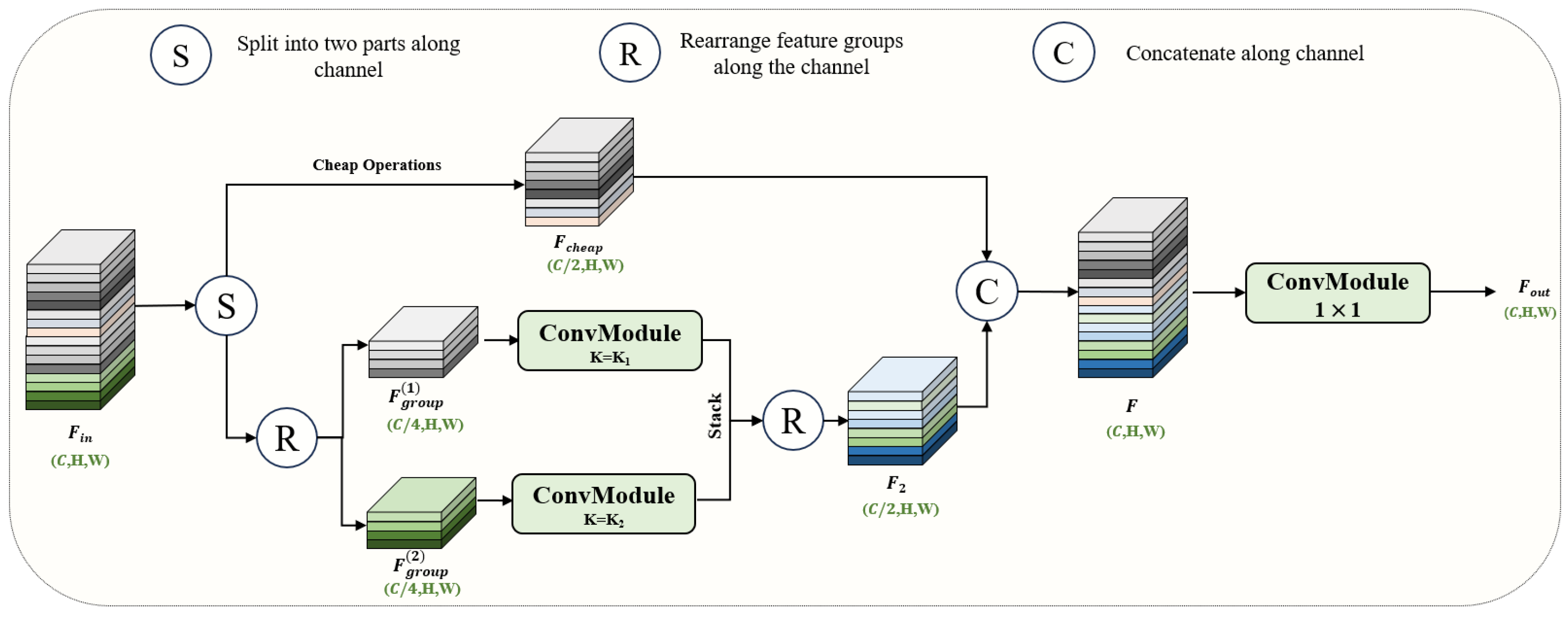
This paper proposes the EGC module to address this issue. This module utilizes grouped convolutions with kernels of varying sizes to decrease the parameter count while also enhancing the capacity to capture multi-scale spatial features and enhancing generalization capability. The structure of the module is shown in Figure 5. Let the input and output of the EGC module be denoted as $F_{in}\in {ℝ}^{C,H,W}$ and $F_{out}\in {ℝ}^{C,H,W}$, where C is the number of channels, and H and W represent the height and width of the feature map. The input feature map F_in is split along the channel dimension into two paths: $F_{cheap}\in {ℝ}^{C/2,H,W}$ and $F_{group}\in {ℝ}^{C/2,H,W}$. After splitting, the dimensions of the feature maps are as follows:

$$F_{cheap}=F_{in}\left[:{\displaystyle \frac{1}{2}}C,\cdots \right],F_{group}=F_{in}\left[{\displaystyle \frac{1}{2}}C:,\cdots \right]$$

(2)

where “:” is used to indicate slicing operations across dimensions.

In the EGC, one path (F_cheap) performs a simple operation to retain the original features, reducing redundancy in the feature mapping, as shown in Figure 6. The other path (F_group) undergoes group convolution, where F_group is split into two groups: $F_{group}^1,F_{group}^2\in {ℝ}^{C/4,H,W}$. These are used as input for the group convolution, which, after processing and feature fusion, generates $F_2\in {ℝ}^{C/2,H,W}$. Finally, a pointwise convolution is applied to merge the feature channels from both paths, resulting in the fused output as:

$$\begin{array}{c}{F}_{out}=Con{v}_{1\times 1}\left(Concat\left(F_{cheap},F_2\right)\right)\end{array}$$

(3)

By applying the EGC module for convolutional operations, the number of input and output channels is reduced to one-quarter of the original size, which subsequently decreases the parameter count accordingly. Equation (4) illustrates how the parameter count might be written as follows:

$$\begin{array}{c}{P}_{EGC}={{\displaystyle \sum }}_{i=1}^G\left(C_{\min \_in}\times C_{\min \_out}\times K_i\times K_j\right)\end{array}$$

(4)

where C_{min_in}, C_{min_out} represent the number of channels after the split operation. G denotes the number of groups. K_i and K_j allude to the grouped convolution kernels’ width and height, respectively.

The receptive field for recognizing image features is directly impacted by the convolution kernel’s size. A well-chosen convolution kernel can improve both the model’s performance and accuracy.

Table 1. Convolution kernels of different sizes.

Kernel Size	Parameters	GFLOPs
NONE	3,006,038	8.1
[1, 3]	2,643,798	7.5
[1, 5]	2,698,406	7.7
[1, 7]	2,772,134	7.8
[3, 5]	2,722,982	7.7
[3, 7]	2,791,254	7.7
[5, 7]	2,847,794	7.9

demonstrates the parameter and computation costs for different kernel sizes. By combining 1 × 1 and 3 × 3 kernels, it is possible to maintain model performance while improving efficiency. Therefore, this study adopts the [1, 3] kernel combination to optimize model performance.

(2)

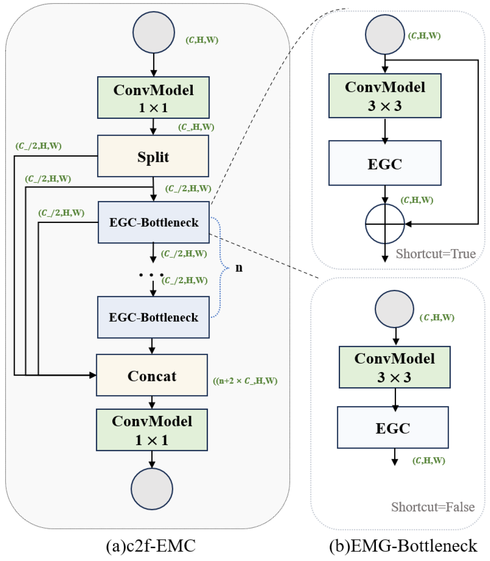
C2f-EGC Module

In the YOLOv8 model, the C2f module primarily extracts higher-level feature representations [28]. Its core comprises convolution layers, activation functions, and Bottleneck modules [29]. This study replaces the second standard convolution module in the Bottleneck with the EGC module, forming the EGC-Bottleneck module (as shown in Figure 7b) to promote the exchange of multi-scale information within the model and capture local contextual information. By stacking multiple EGC-Bottleneck modules, a new network structure, C2f-EGC, is constructed (as shown in Figure 7a).

In convolution layers with high channel numbers (128 and above), the C2f-EGC model replaces the original C2f module in this study. For layers with lower channel numbers (less than 128), the impact of grouped convolution is minimal, so the original C2f module is retained.

Table 2. Parameter comparison between C2f and C2f-EGC modules.

Model	Layer	Output Channel	Kernel Size	Parameter
C2f	6	128	3 $\times$ 3	197,632
	8	256	3 $\times$ 3	460,288
	12	128	3 $\times$ 3	148,224
	18	128	3 $\times$ 3	123,648
	21	256	3 $\times$ 3	493,056
C2f-EGC	6	128	[1, 3]	137,344
	8	256	[1, 3]	339,584
	12	128	[1, 3]	118,080
	18	128	[1, 3]	93,504
	21	256	[1, 3]	372,352

compares the parameter counts between the C2f and C2f-EGC modules for high-channel layers. The results show that the C2f-EGC module reduces parameter count by more than 20% without compromising feature extraction capability.

2.2.2. Group Context Anchor Attention

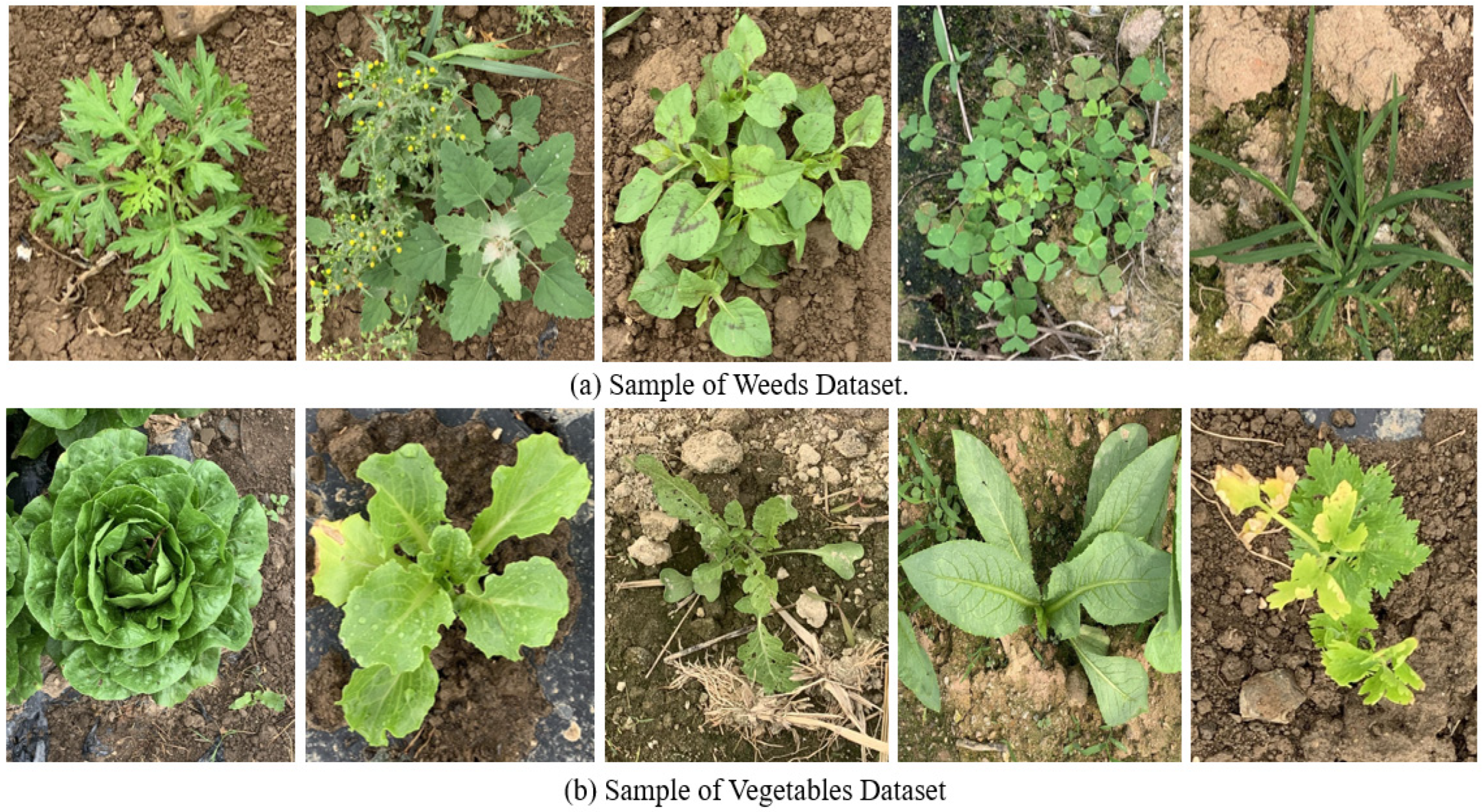
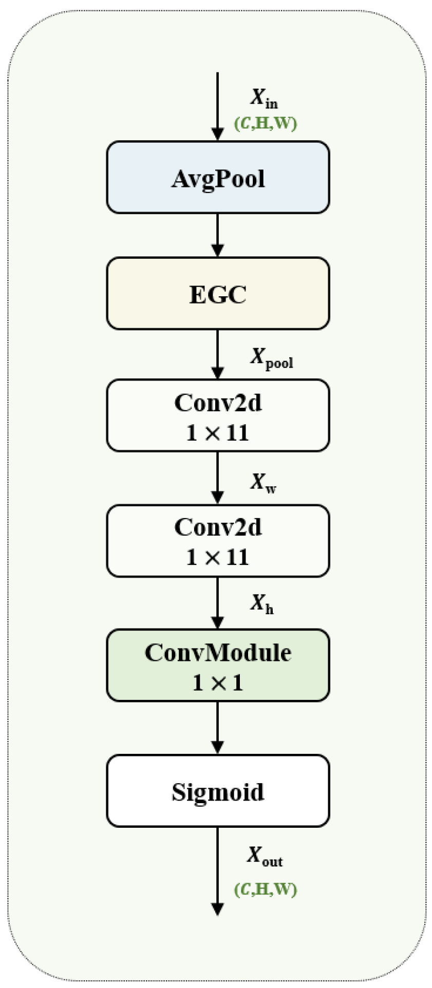
In object detection, local information can be impacted by local blurring or noise, leading to decreased model performance. In vegetable and weed recognition, vegetables are typically planted in an organized manner, while weeds are randomly distributed [30,31]. This paper introduces the Group Context Anchor Attention (GCAA) mechanism, consisting primarily of pooling layers, EGC modules, depth-wise separable convolutions, and activation functions. The GCAA is intended to enhance the spatial feature representation for both weeds and vegetables by increasing the model’s ability to capture long-range contextual information.

Figure 8 illustrates the GCAA model’s structure. First, an average pooling operation is applied to local regions, which averages out the local features, extracts global features, and reduces the dimensionality of the feature map. The local region’s features are then obtained using the EGC convolution procedure. The operation formula is as follows:

$$\begin{array}{c}{X}_{pool}=EG{C}_{i\times i}\left({\mathcal{P}}_{avg}\left(X_{in}\right)\right)\end{array}$$

(5)

where EGC_i×i represents the convolution operation of the EGC module with $i\in \left[1,3\right]$, indicating a convolution kernel size of [1, 3]. ${\mathcal{P}}_{avg}$ represents the average pooling operation. $X_{in}$ represents the input value.

Then, depth-wise separable convolution is applied to capture long-range dependencies in both horizontal and vertical directions. Large convolution kernels of size 1 × 11 and 11 × 1 are used to perform convolutions along the vertical and horizontal axes. The operation is formulated as:

$$X_w=Con{v}_{1\times 11}(X_{pool})$$

(6)

$$X_h=Con{v}_{11\times 1}(X_w)$$

(7)

where $X_w$ and $X_h$ represent the output values after the 1 × 11 and 11 × 1 convolutions. Conv represents the standard convolution operation.

Finally, a pointwise convolution is used to integrate and compress the features extracted from the separable convolution (X_h) along the channel dimension. The sigmoid activation function is applied to perform a nonlinear transformation, generating the output feature X_out as shown in Equation (8). For the feature fusion that follows, it is crucial to make sure that the output feature values fall between 0 and 1.

$$\begin{array}{c}{X}_{out}=\sigma \end{array}\left(Con{v}_{1\times 1}\left(X_h\right)\right)$$

(8)

where $\sigma$ denotes the sigmoid function.

2.2.3. GCAA-Based Feature-Level Fusions Model

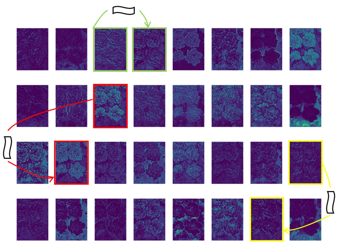
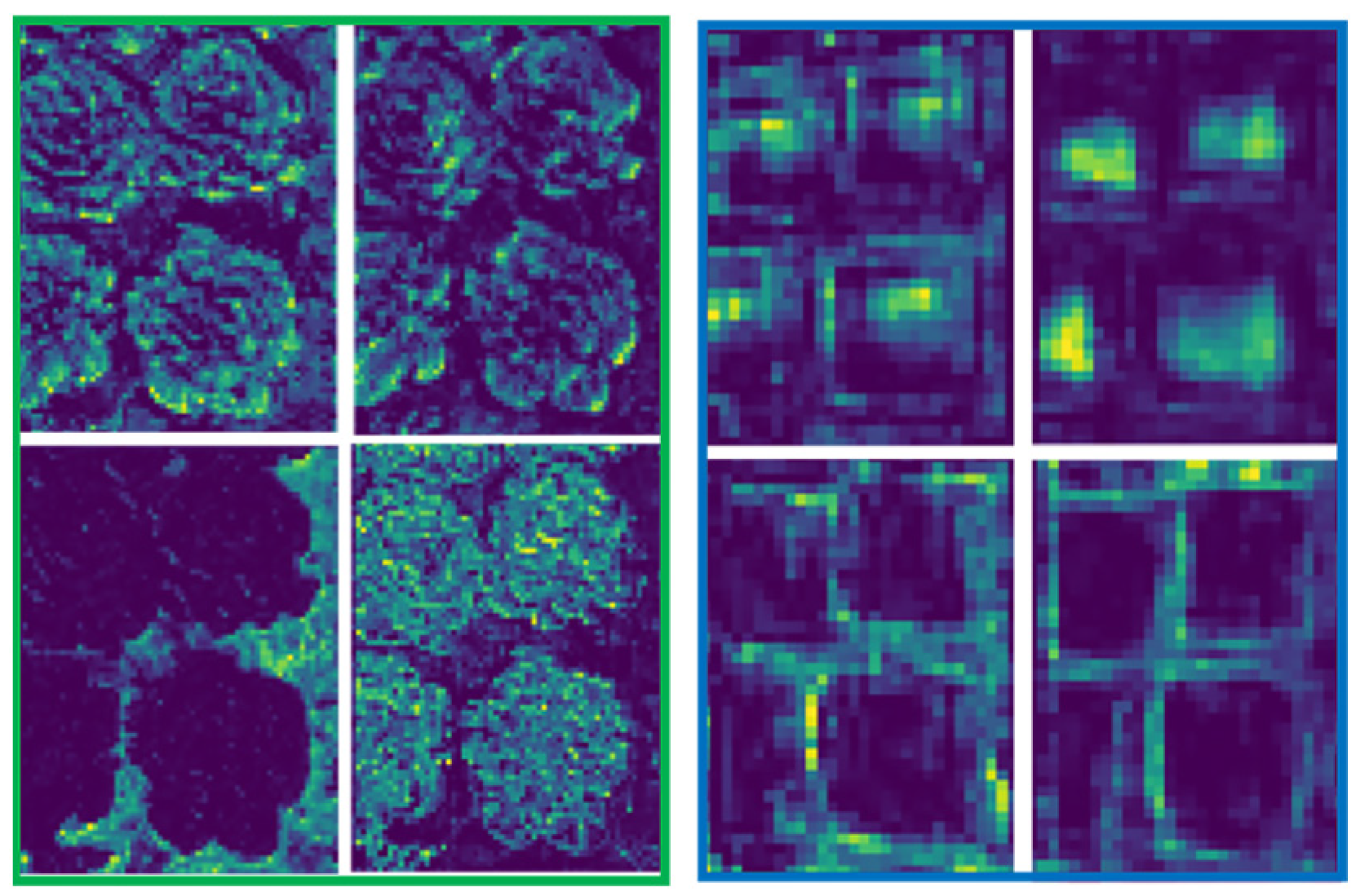
Shallow feature maps contain rich low-level information, such as edges and textures, which can effectively distinguish subtle differences between vegetables and weeds. However, during the object detection process, consecutive convolution and pooling operations reduce the resolution of deep feature maps, resulting in the loss of shallow information. Deep networks primarily extract abstract features such as object categories, negatively impacting the recognition of small objects and targets with similar shapes, as illustrated in Figure 9 [32,33].

We assessed the Peak Signal-to-Noise Ratio (PSNR) and Structural Similarity Index (SSIM) for images of various resolutions, as stated in Equations (9) and (10), aiming to examine better how image resolution affects feature extraction and object detection accuracy [34].

$$\mathrm{PSNR}=10\cdot {\log }_{10}({\displaystyle \frac{MA{X}^2}{MSE}})$$

(9)

where MAX is the maximum pixel value of the image, and MSE is the Mean Squared Error between two images. A higher PSNR value indicates better image quality.

$$SSIM(x,y)={\displaystyle \frac{(2{\mu }_x{\mu }_y+C_1)(2{\sigma }_{xy}+C_2)}{({\mu }_x^2+{\mu }_y^2+C_1)({\sigma }_x^2+{\sigma }_y^2+C_2)}}$$

(10)

where ${\mu }_x$ and ${\mu }_y$ are the means of images x and y, ${\mu }_x^2$ and ${\mu }_y^2$ are their variances, ${\sigma }_{xy}$ is the covariance, $C_1$ and $C_2$ are constants to stabilize the division. Higher scores on the SSIM scale, which goes from 0 to 1, indicate more remarkable similarity.

The results are summarized in

Table 3. PSNR and SSIM values for different image sizes.

Image Size	PSNR	SSIM
320 × 320	24.00	0.80
160 × 160	21.65	0.73
80 × 80	19.79	0.69
40 × 40	18.20	0.67

. As the image resolution decreases, PSNR and SSIM values decline, indicating a loss of information and structural similarity. Lower-resolution images lose finer details, which potentially degrades deep networks’ ability to distinguish objects.

Feature enhancement is key to solving the problem of feature disappearance. In previous object detection algorithms, attention mechanisms are often used to highlight key features, which is effective but still faces the challenge of balancing and preserving low-level details and capturing high-level contextual information.

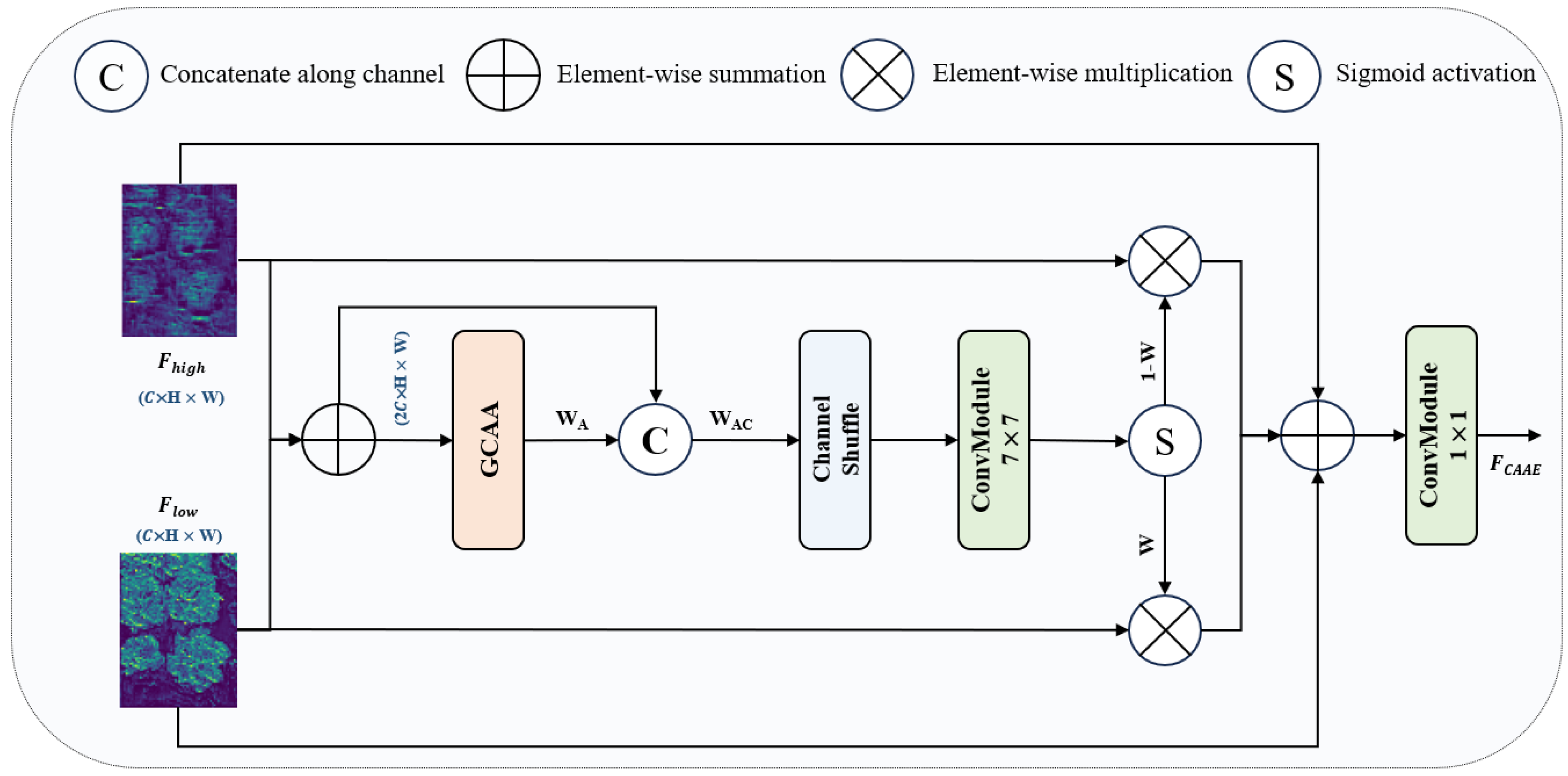
To address this issue, this paper introduces a feature fusion module based on GCAA (GCAA-Fusion). The module adaptively merges shallow and deep feature maps, enhancing both feature preservation and gradient backpropagation. As shown in Figure 10, the low-level feature map $F_{low}\in {ℝ}^{C,H,W}$ is combined with the high-level feature map $F_{high}\in {ℝ}^{C,H,W}$ through simple addition. The combined features are then passed through the GCAA attention module to generate an initial attention map $W_A\in {ℝ}^{C,H,W}$, integrating long-range contextual information with detailed features, as expressed in Equation (11).

$$\begin{array}{c}{W}_A=GCAA\left(F_{low}\oplus F_{high}\right)\end{array}\in {ℝ}^{C,H,W}$$

(11)

where $\oplus$ represents the element-wise summation.

To obtain a more precise saliency feature map, the initial attention feature map $W_A$ is first concatenated with the original feature map after the addition operation to form $W_{AC}\in {ℝ}^{C,H,W}$. Then, channel shuffle operations are applied to rearrange the channels of $W_{AC}$ alternately. Finally, a 7 × 7 convolution operation followed by an activation function is applied to produce the feature weights $W$. The computation process is shown in Equations (12) and (13).

$$\begin{array}{c}{W}_{AC}=concat\left(W_A,\left(F_{low}\oplus F_{high}\right)\right)\end{array}$$

(12)

$$\begin{array}{c}W=\sigma (Con{v}_{7\times 7}\left(CS\left(W_{AC}\right)\right)\end{array}$$

(13)

where CS(·) refers to the channel shuffle operation. $Con{v}_{7\times 7}$ depicts the convolution operation using a kernel size of 7 × 7.

The precise feature maps generated through weighted summation are then integrated, with skip connections introduced to enhance the input features. This helps mitigate the vanishing gradient problem and simplifies the training process. Given that shallow and deep features complement each other, the generated weight W is applied to one module, while the fusion weight for the other module is represented as 1 − W [33]. Based on this, the fused features are mapped using a 1 × 1 convolution layer to obtain the final feature output, as indicated in Equation (14).

$$\begin{array}{c}{F}_{CAAE}=Con{v}_{1\times 1}\left(F_{low}\otimes W\oplus F_{high}\otimes (1-W)\right)\oplus F_{low}\oplus F_{high}\end{array}$$

(14)

where $\otimes$ represents the elementwise multiplication.

2.2.4. Adaptive Feature Fusion (AFF)

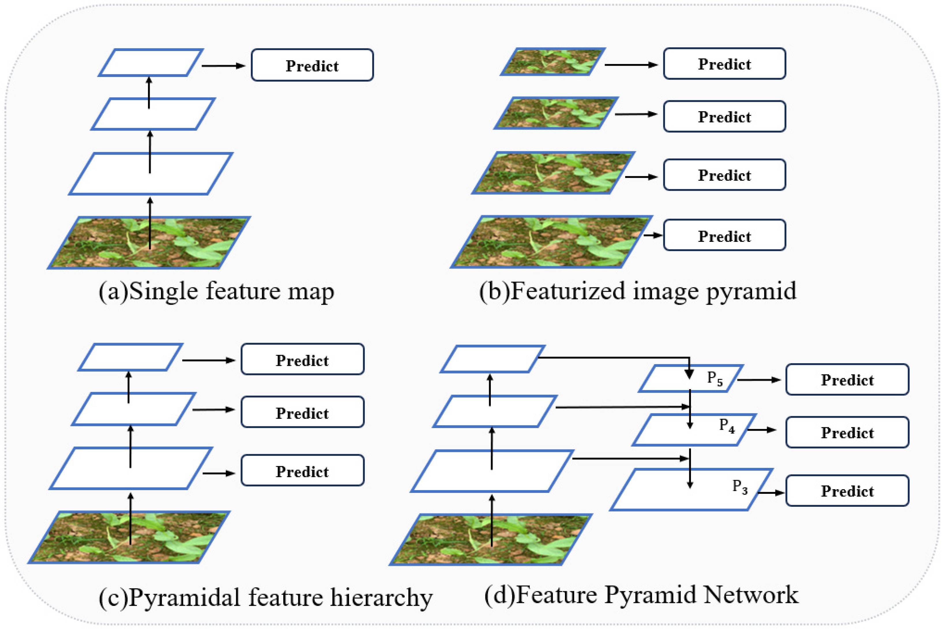
The Feature Pyramid is crucial in object detection for capturing multi-scale features. Figure 11 outlines different pyramid structures. In Figure 11a, a single feature map is used for prediction, limiting the ability to exploit multi-scale information. Figure 11b presents an image pyramid approach where feature maps are generated at each scale, but this incurs a high computational cost [35]. Figure 11c enhances detection performance by utilizing multi-layer feature extraction [36], though it may lack precision in capturing fine details. Figure 11d focuses on resolving the multi-scale challenge in object detection while reducing computational complexity, although efficiency could still be optimized [37]. Improving feature extraction methods can substantially enhance the network’s detection accuracy. YOLOv8 employs the Path Aggregation Feature Pyramid Network (PAFPN) to facilitate information fusion across different layers, but deeper network layers can lead to feature loss.

This paper introduces an AFF structure built upon the PaFPN architecture to address the issue. As shown in Figure 4 and Figure 12, The orange dashed lines correspond to the 9th, 6th, and 4th layers, and the output layers N5, N4, and N3 correspond to the 15th, 18th, and 21st layers, respectively. Three GCAA-Fusion modules are incorporated before each Detection Head, with their inputs sourced from the 4th and 15th layers, the 6th and 18th layers, and the 9th and 21st layers. The AFF structure adaptively merges low-level and high-level features along the channel dimension, increasing the model’s ability to preserve features and raising object detection’s precision and effectiveness. This results in greater robustness and adaptability across various tasks.

2.3. Experimental Platform and Parameter Configuration

The experimental platform operates on a Windows 10 system, equipped with an NVIDIA Quadro RTX 5000 GPU (NVIDIA, Santa Clara, CA, USA), Intel(R) Xeon(R) Gold 6248R @ 3.00 GHz CPU (Intel, Santa Clara, CA, USA), and 64.0GB of RAM (Kingston, Fountain Valley, CA, USA). PyTorch is the deep learning framework used, with CUDA 11.6 serving as the parallel computing platform and programming model. Python 3.9 is employed as the programming language.

Most of the experiment’s parameters retain YOLOv8’s default settings. The batch size is 32, the number of workers is 5, and the input image size is fixed at 640 × 640 pixels. The weight decay is 0.0005, the momentum is 0.937, and the learning rate is 0.01.

Table 4. Hyperparameter information.

Hyper Parameters	Values
Epochs	400
Batch Size	32
Workers	5
Imgsz	640
Learning Rate	0.01
Momentum	0.937
Weight Decay	0.0005

provides detailed information about the hyperparameter settings.

2.4. Metric

The evaluation of network performance primarily relies on mAP (Mean Average Precision) during the training process and the model’s performance on the validation set after training. To assess the model’s performance, five key metrics are used in this paper: precision, recall, mAP, F1 score, and parameters. The corresponding calculation formulas are as follows:

$$\begin{array}{c}Precision={\displaystyle \frac{True Positives}{True Positives+False Positives}}\end{array}$$

(15)

$$\begin{array}{c}Recall={\displaystyle \frac{True Positives}{True Positives+False Negatives}}\end{array}$$

(16)

$$\begin{array}{c}F1score=2{\displaystyle \frac{Precision\cdot Recall}{Precision+Recall}}\end{array}$$

(17)

where True Positives represent the quantity of actual weed samples accurately classified by the model as weeds. False Positives represent the number of actual non-weed samples mistakenly identified by the model as weeds. False Negatives represent the number of actual weed samples incorrectly identified by the model as non-weeds.

mAP is a crucial performance evaluation metric that calculates the mean of the average precision (AP) across all categories, as illustrated in Equations (18) and (19). mAP0.5 denotes the mAP value when the Intersection over Union (IoU) is set to 0.5. mAP0.5–0.95 refers to the mAP evaluated at various IoU thresholds ranging from 0.5 to 0.95, with an increment of 0.05 [38].

$$AP={{\displaystyle \int }}_0^{1}Precision\left(Recall\right)dr$$

(18)

$$mAP={\displaystyle \frac{1}{N}}{\displaystyle \sum _{i=1}^{N}AP}$$

(19)

where N represents the classification categories in this paper.

3. Results and Discussion

3.1. Performance Experiments

This study conducts experiments with varying counts of GCAA-Fusion modules to evaluate the impact of the AFF network architecture on YOLOv8n model performance while keeping other parameters fixed. Fusion-1 represents the YOLOv8n model enhanced with a single GCAA-Fusion module, while Fusion-2 incorporates two GCAA-Fusion modules. Results in

Table 5. Results of the YOLOv8 with varying numbers of GCAA-Fusion modules.

Models	Precision (%)			Recall (%)			mAP0.5 (%)			mAP0.5–0.95 (%)			F1 (%)
	Weed	Crop	All	Weed	Crop	All	Weed	Crop	All	Weed	Crop	All	All
YOLOv8	87.1	92.7	89.4	80.7	94.6	87.8	88.5	96.8	92.7	61.6	84.4	72.9	88.5
Fusion-1	86.4	92.2	89.3	80.8	95.7	88.2	88.3	97.1	92.6	60.7	84.8	72.8	88.7
Fusion-2	87.8	93	90.4	80.2	95.1	87.7	88.5	97.1	92.8	61.2	84.8	73	89.1
YEF	87.9	93	90.4	80.8	95.4	88	88.8	97.1	92.9	61.5	84.4	73.3	89.1

indicate that adding GCAA-Fusion modules leads to measurable improvements across detection metrics compared to the baseline YOLOv8n model. Notably, with the addition of three GCAA-Fusion modules (YEF), the model achieves optimal results across all evaluation metrics, highlighting the significant performance enhancements provided by the AFF network architecture.

This study substitutes the GCAA attention mechanism within the GCAA-Fusion module with alternative attention mechanisms—MLCA [38], CBAM [39], SE [40], and EMA [41]—to form new feature fusion modules and further assess the impact of feature fusion on the model.

The results, presented in

Table 6. Model performance metrics with different feature fusion modules.

Models	Precision (%)			Recall (%)			mAP0.5 (%)			mAP0.5–0.95 (%)			F1 (%)
	Weed	Crop	All	Weed	Crop	All	Weed	Crop	All	Weed	Crop	All	All
MLCA	88.5	93.1	90.8	80.1	95.3	87.7	88.3	97.1	92.7	61.3	85.2	73.1	89.2
EMA	86.8	92.6	89.7	81.2	94.3	87.8	88.9	96.4	92.7	61.3	84.6	72.9	88.7
CBAM	88.2	94.1	91.1	79.3	94.9	87.1	88.5	97.2	92.9	61.1	85.2	73.2	89.0
SE	85.8	92.3	89	81.6	95.2	88.4	88.7	96.8	92.8	60.8	84.9	72.8	88.7
None	87.1	92.7	89.4	80.7	94.6	87.8	88.5	96.8	92.7	61.6	84.4	72.9	88.5
GCAA	87.9	93	90.4	80.5	95.4	88	88.8	97.1	92.9	61.5	84.4	73.3	89.1

, demonstrate that all feature fusion modules improve detection metrics over the baseline YOLOv8n model, validating the feasibility and robustness of the proposed feature fusion framework. The F1 score shows the most significant improvement among all metrics, indicating that feature fusion better balances precision and recall.

Moreover, the GCAA-based fusion module consistently outperforms other attention mechanisms, achieving the highest mAP scores. This highlights the strength of the GCAA mechanism in optimizing feature representation by combining high-level and low-level features. Additionally, different attention mechanisms display unique advantages for specific metrics; for example, SE excels in improving recall, while CBAM achieves competitive performance across most metrics. These attention mechanisms bring unique characteristics suited to different tasks, enabling flexibility in selecting fusion modules based on specific recognition targets.

Figure 13 illustrates the mAP0.5 values over training epochs for models with different fusion modules. In the early training stages, mAP values across fusion modules are similar; however, in later stages, all fusion-enhanced models surpass the baseline, with the GCAA-Fusion module yielding the highest mAP0.5 value, underscoring its superior detection performance relative to other fusion methods.

3.2. Comparative Experiments with the Original Model

This study presents enhancements to the YOLOv8 model’s feature extraction and fusion techniques. Various comparison studies were created to evaluate the efficacy of these changes. First, using the same dataset, the YEF model’s detection performance was compared to that of the original YOLOv8n model; the results are displayed in

Table 7. Comparison of detection results between YEF and original model.

Models	Parameters	Class	Precision (%)	Recall (%)	mAP0.5 (%)	mAP0.5–0.95 (%)	F1 (%)
YEF	3.0 M	Weed	87.9%	80.5%	88.8%	61.5%	84.0%
		Crop	93%	95.4%	97.1%	85.1%	94.1%
		All	90.4%	88%	92.9%	73.3%	89.1%
YOLOv8n	3.0 M	Weed	87.1%	80.7%	88.5%	61.6%	83.7%
		Crop	92.7%	94.6%	96.8%	84.4%	93.6%
		All	89.4%	87.8%	92.7%	72.9%	88.5%

. As indicated, the YEF model outperforms YOLOv8n in all metrics across all categories without increasing the parameter count. Notably, the accuracy reaches 90.4%, representing a 1% improvement over the original model. Other metrics also show varying degrees of improvement, demonstrating that the modifications effectively enhance detection performance.

Grad-CAM is a technique that visualizes the intensity distribution of features through color changes, where brighter colors indicate greater attention [42]. Grad-CAM is used in this work to illustrate the YEF model’s detection results. As illustrated in Figure 14, the shallow network layer (layer 5) emphasizes detailed information, such as edges, textures, and object outlines. With the addition of the C2f-EGC module in the Backbone network, the model’s semantic understanding of the plants is significantly enhanced. The 12th layer (small object detection layer) effectively captures fine features of small objects, while the most critical 24th layer (fusion layer), enhanced by the GCAA-Fusion module, further improves the integration capability of multi-scale features.

These visualizations confirm that the improvements in the YEF model enhance feature representation. By effectively capturing both high-level semantic features and low-level details, the model is able to better represent the objects, leading to more accurate detection and localization. This ability to leverage both types of features, particularly in challenging environments, results in more precise and robust performance.

To further demonstrate the generalizability of the proposed EGC and GCAA-Fusion modules, the EGC module was embedded within the C3 module of YOLOv5, forming the C3-EGC module. Additionally, the GCAA-Fusion module was integrated for enhanced feature fusion, resulting in a new model architecture named YEF-5. Comparative experiments were conducted to evaluate the detection performance of YEF-5 against the YOLOv5n baseline.

According to

Table 8. Detection results of the YEF-5 model compared to the YOLOv5n model.

Models	Precision (%)			Recall (%)			mAP0.5 (%)			mAP0.5–0.95 (%)			F1 (%)
	Weed	Crop	All	Weed	Crop	All	Weed	Crop	All	Weed	Crop	All	All
YOLOv5n	85.6	92	88.8	80.6	95	87.8	88.4	96.6	92.5	60.3	84.4	72.4	88.2
YEF-5	86.5	93.3	89.9	81.3	95.4	88.5	88.7	96.9	92.8	60.3	84.5	73.4	89.1

, the findings reveal that YEF-5 consistently outperforms YOLOv5n across all evaluation metrics. Figure 15 illustrates the evolution of mAP0.5 over training epochs. Although YEF-5 initially shows a slightly lower mAP than YOLOv5n, it eventually surpasses the baseline as training progresses. This trend suggests that YEF-5 requires a more extended adjustment period during early training but ultimately excels in capturing critical data features, leading to superior performance in later stages.

These findings highlight the positive impact of the introduced modules on model performance, demonstrating their adaptability across different architectures and confirming their effectiveness in both YOLOv8n and YOLOv5n frameworks. These findings imply that the proposed improvement methods and modules could be generalized to a wide range of object detection models, potentially benefiting agricultural applications.

3.3. Comparative Experiments with the Other Model

The benefits of the YEF model in vegetable weed recognition tasks were assessed in this study by conducting comparative experiments on the same dataset against several well-known object detection algorithms. First, it was compared with the classic two-stage Faster R-CNN model, followed by the classic single-stage RetinaNet model. Next, comparisons were made with the end-to-end DINO model, the lightweight models RTMDet-Tiny and YOLOv10n, and finally, the TOOD-R50 model [43,44,45,46].

According to the data in

Table 9. Detection results of the YEF model compared with other models.

Models	Parameters	Precision (%)	Recall (%)	mAP0.5 (%)	mAP0.5–0.95 (%)
Faster R-CNN	41 M	71.1%	90%	81.5%	65.4%
TOOD-R50	321 M	71.4%	91.4%	83.3%	69.7%
RTMDet-Tiny	4 M	73.1%	91.3%	81.3%	64.7%
RetinaNet	36 M	60.3%	87.6%	77.5%	63.7%
DINO	47 M	86.4%	87%	89%	70.3%
YOLOv10	2.76 M	89%	87%	91%	72.1%
YEF	3 M	90.4%	88%	92.9%	73.3%

and the comparison experiment results, the YEF model outperforms other models in several key metrics. Among the models tested, the YEF model achieves the highest precision (90.4%), mAP0.5 (92.9%), and mAP0.5–0.95 (73.3%). Notably, TOOD-R50 and DINO deliver impressive detection results with mAP0.5 values of 83.3% and 89%, respectively, but their parameter counts are significantly higher—321 M and 47 M, respectively—compared to the YEF model’s lightweight 3 M. Similarly, YOLOv10, a compact model with 2.76 M parameters, achieves strong precision (89%) and mAP0.5 (91%), but it still falls short of the YEF model across all metrics.

These results underscore the YEF model’s capability for accurate and efficient detection, making it particularly suitable for agricultural applications. Future work could focus on optimizing the model for better deployment efficiency in resource-constrained environments.

3.4. Qualitative Results

This study utilized publicly available weed datasets to evaluate the detection performance of the YEF model to verify the reliability and generalizability of the proposed model. The first dataset employed was the publicly available sesame weed dataset [47], which comprises 1300 images of sesame crops and various types of weeds, with each image sized at 512 × 512 pixels.

Table 10. Detection results of the YEF model on the sesame weed dataset.

Types of Weeds	Precision (%)	Recall (%)	mAP0.5 (%)	mAP0.5–0.95 (%)	F1 (%)
All	86.1	82.7	89	56.9	84.3
Weed	93.4	84	91.9	54.4	88.4
Crop	78.7	81.5	86.1	55.1	80.0

presents the detection results of the YEF model, showing an overall precision of 86.1%, a recall rate of 82.7%, a mAP at IoU 0.5 of 89%, and a mAP at IoU 0.5–0.95 of 56.9%. Specifically, for different types of weeds, the model achieved a precision of 93.4% and a recall rate of 84%.

The second dataset utilized is the largest public weed detection dataset currently available in cotton production systems [48]. This dataset includes 12 common types of weeds found in cotton fields, comprising 5648 images and 9370 bounding boxes.

Table 11. Detection results of the YEF model on the cotton weed dataset.

Types of Weeds	Precision (%)	Recall (%)	mAP0.5 (%)	mAP0.5–0.95 (%)	F1 (%)
all	92.1	89.4	93.6	88	90.7
eclipta	95.1	96.8	99.1	97.9	95.9
ipomoea indica	97.2	92.4	96.2	88.7	94.5
eleusine indica	93.5	90.1	93.8	84.5	87
sida rhombifolia	91	92	95.1	92.3	91.4
physalis angulata	85.2	71.4	77.8	73.8	77.6
senna obtusifolia	95.4	100	99.5	98.7	97.6
amaranthus palmeri	94.4	92.3	96.3	94.5	93.3
euphorbia maculata	95.7	85	91.4	83.5	90
portulaca oleracea	89.1	90.9	95.3	86.3	89.9
mollugo verticillata	84.9	81.2	88.9	80.4	83
amaranthus tuberculatus	96.2	92.2	97.2	92.5	94.1
ambrosia artemisiifolia	88.1	88.2	92.5	82.6	88.1

presents the detection results of the YEF model for various weed types, demonstrating superior identification capabilities across most categories. For instance, the precision for Eclipta reached 95.1%, with a recall rate of 96.8%. The results from both datasets indicate that the YEF model exhibits strong detection performance when handling different types of weed datasets, thereby proving its effectiveness and reliability for practical applications.

As shown in Figure 16, the qualitative detection results demonstrate the YEF model’s ability to accurately identify crops and weeds under various challenging conditions, including complex backgrounds, diverse plant types, and varying object sizes. (a) illustrates an example containing both vegetables and weeds, (b) shows a weed-only target, and (c) focuses solely on vegetable targets. This comprehensive representation highlights the model’s adaptability to different detection scenarios.

4. Conclusions

This paper presents a vegetable and weed detection model, YOLOv8-EGC-Fusion (YEF), capable of distinguishing crops from weeds in various complex environments. The model introduces three plug-and-play modules: EGC, GCAA, and GCAA-Fusion. The EGC module employs convolution kernels of varying sizes for efficiently grouped convolution, enabling the capture of spatial features at different scales, and it combines with the C2f module to form the C2f-EGC module. Utilizing the C2f-EGC module with a high number of channels enhances the network’s capacity to acquire local contextual information. The GCAA module leverages separable convolutions to obtain long-range contextual information. The GCAA-Fusion module effectively merges shallow and deep features, addressing the issue of feature loss within the network. Additionally, this paper designs a new feature pyramid structure—AFF—based on GCAA-Fusion and PAFPN, which further improves the model’s feature extraction capabilities.

The efficiency of the suggested model was successfully tested through several studies. Comparative experiments against the original model and mainstream network models demonstrate that the YEF model excels in recognition tasks, effectively addressing the difficulties associated with multi-scale object detection, and outperforms the YOLOv8n model, as well as mainstream networks such as Faster R-CNN, RetinaNet, Tood, RTMdet, and YOLOv5 in key metrics like precision, recall, and mAP. Results from comparative experiments on feature fusion modules with different attention mechanisms indicate that the feature fusion module based on the GCAA attention mechanism significantly enhances the algorithm’s expressiveness and detection performance. Incorporating the improved modules into the YOLOv5 model and proving their effectiveness through comparative experiments shows that the proposed modules demonstrate strong generalizability, significantly enhancing the recognition capability of YOLOv5. Testing the YEF model on public datasets confirmed its outstanding performance across different scenarios and target conditions, achieving the expected objectives.

The YEF model has shown promising results in vegetable and weed detection tasks and holds potential for practical applications in agriculture; however, it still has certain limitations: (1) the model requires further optimization for speed and memory usage prior to hardware deployment, and (2) the model has only been tested for a limited number of vegetables and weeds, while actual agricultural production involves a greater variety of vegetables and more complex planting environments. Therefore, further research and validation of the model’s effectiveness for other vegetables and weeds is needed.