Article

Propagation Laws of Ultrasonic Continuous Signals at the Transmitting Transducer–Soil Interface

1
College of Engineering, China Agricultural University, Beijing 100083, China
2
Scientific Observing and Experiment Station of Arable Land Conservation (North Hebei), Ministry of Agricultural and Rural Affairs, Beijing 100083, China
*
Author to whom correspondence should be addressed.
Agriculture 2024, 14(9), 1470; https://doi.org/10.3390/agriculture14091470
Submission received: 19 July 2024 / Revised: 21 August 2024 / Accepted: 27 August 2024 / Published: 28 August 2024
(This article belongs to the Section Agricultural Soils)

Abstract

:
Ultrasonic detection is one of the main methods for information detection and has advantages in soil detection. Ultrasonic signals attenuate in soil, resulting in unique propagation laws. This paper studies the propagation laws of ultrasound in soil, focusing on the propagation characteristics of ultrasonic continuous signals at the transducer–soil interface. This study uses excitation frequency and amplitude as experimental factors and employs the discrete element simulation method to analyze the vibration characteristics of soil particles. It reveals the relationship between changes in soil pressure at the interface and the movement of the transducer. The results show that the motion curve of the transmitting transducer lags behind the soil pressure changes, and the energy of the ultrasonic signal increases with higher excitation frequency and amplitude. Specifically, the peak value of the first wave |H0| at 40 kHz and 60 kHz is 210% and 263% of that at 20 kHz, respectively. When the excitation amplitude increases from 0.005 mm to 0.015 mm, the value of the peak value of other waves |H| increases by 323%. This paper preliminarily reveals the propagation laws of ultrasonic continuous signals at the transducer–soil interface, providing theoretical support for the development of ultrasonic soil property detection instruments.

1. Introduction

Ultrasonic detection is a key method for information gathering and has been widely used in various fields, including metal flaw detection [1], parameter measurement [2], civil engineering safety assessments [3], and damage evaluation of ancient buildings [4,5]. This technique boasts several advantages, such as safety [6], environmental friendliness, low energy consumption, the lack of need for external additives, and ease of use. Additionally, ultrasound can propagate through opaque materials and has non-destructive properties [7]. Consequently, the application of ultrasound across different domains has emerged as a significant research focus in recent years [8].
The ultrasonic method also has many applications in agriculture, such as the use of ultrasound to judge the hollow and disease of potatoes [9], to identify corn stalks [10], to pollinate strawberries [11], and to determine the maturity of fruits [12]. Soil information, including soil temperature, moisture, and soil compaction, is one of the main components of agricultural information [13,14,15,16,17]. Soil information can be obtained by the ultrasonic method. Baskota et al. [18] studied a single-chip GHz ultrasonic micro-imager for imaging soil temperature, morphology, moisture, and pests. Zhang et al. [19] measured the freezing state of soil by the ultrasonic method. The study of Zhang et al. [20] shows that with the increase in pore equivalent diameter, the ultrasonic pulse velocity decreases slightly at first, and then rises greatly. The results of Zhao et al. [21] show that it is feasible to use the ultrasonic pulse velocity test to detect the hard foreign object embedded in the farmland layer according to the variation in the ultrasonic wave propagation velocity and the amplitude of the sound wave in the soil medium. Compared to existing soil detection methods that require digging up soil or bringing it back to the laboratory for detecting, the ultrasonic method supports in situ detection, is easy to operate [22], and is one of the important means of efficient detection.
This paper aims to provide foundational research for various ultrasonic soil detection technologies. When using ultrasonic methods to detect soil properties, it is necessary for the ultrasonic signal to propagate through the soil, but this presents certain challenges. Soil is a porous medium composed of minerals, organic matter, water, and air, making it a complex and randomly varying dispersive mixture. Compared to continuous media, the looseness of the soil and the fluids in its pores lead to greater energy loss of ultrasonic signals, resulting in significant attenuation [23]. The interface, being the junction between two substances, is a key location where attenuation occurs [24]. As the first stage in the propagation of ultrasonic signals in soil, the interface is where the signal transitions from the motion of the ultrasonic transducer to the vibration of the soil. The quality of the signal at the interface directly affects subsequent propagation into the soil, necessitating a dedicated study of the propagation characteristics at the interface. To address the issue of ultrasonic energy loss in soil media, using ultrasonic continuous signals offers advantages. Ultrasonic continuous signals are vibration signals generated by the continuous drive of the transmitting transducer on the soil, forcing soil particles to vibrate persistently under the steady and unified force direction of the transducer. Moreover, because the transmitting time of ultrasonic continuous signals is longer, they carry stronger energy, resulting in greater anti-interference capability as they propagate through the soil medium. The signal shape becomes easier to control, and the receiving end can receive more stable signals, facilitating their reception, processing, and analysis. Additionally, parameters carrying important information in continuous signals are easier to identify after post-processing [25]. Therefore, when the medium is soil, ultrasonic continuous signals may be more suitable for detection. However, there is currently no research on the attenuation laws of continuous signals at soil interfaces. This paper introduces ultrasonic continuous signals as the transmitting signal and studies their propagation characteristics at the interface between the transmitting transducer and the soil to alleviate the problem of energy attenuation.
The interaction between ultrasonic waves and the medium is a microscopic process. To study the laws of vibration propagation among medium particles, it is essential to obtain microscopic data. Currently, many researchers utilize numerical simulation methods to investigate these microscopic processes. This approach allows for the acquisition of process data through computer-aided calculations, facilitating the analysis of localized physical quantities during the interaction. Cho et al. [26] employed the finite element method to predict motor vibration. Shen et al. [27] explored the relationships among P-wave velocity, pre-existing cracks, and confining pressure using the discrete element method (DEM). In soil detection environments, discrete element simulation technology is particularly applicable, enabling the modeling of soil particles and the application of forces or motion to them. This technology has been extensively used by researchers in the agricultural engineering field to examine the interaction mechanisms between working components and soil [28,29]. Xu et al. [30] analyzed the interaction between soil and subsoiling shovel, aiming to clarify the drag reduction mechanism of a bionic subsoiling shovel by through EDEM software. Yang et al. [31] used EDEM software to simulate the spread of commonly used agricultural fertilizers by a fertilizer applicator. Zhou et al. [32] designed a high-efficiency drag-reducing bionic soil-loosening shovel based on EDEM technology. We are studying the propagation characteristics at the ultrasonic incident interface, which is a local aspect of the overall process of ultrasonic wave propagation in soil. Given current technological conditions, it is not feasible to observe this local aspect through practical experiments. Additionally, we need to investigate the microscopic mechanisms and laws of ultrasonic attenuation, which are also challenging to achieve through experiments. Therefore, using simulation methods for research is necessary. The essence of ultrasonic propagation lies in the vibration of the medium, which involves the transmission of forces and the movement of the medium itself. In order to fully analyze the propagation process of sound wave in soil medium and study the vibration of soil particles, this paper employs discrete element simulation software (EDEM 2018) to simulate the propagation process and results of ultrasonic waves within the soil. By tracking designated particles and extracting their target data, we can observe the microscopic phenomena associated with vibration propagation.
In conclusion, the ultrasonic method offers significant advantages for soil detection. To minimize the energy attenuation of ultrasonic signals in soil, this paper studies the propagation laws of ultrasonic continuous signals at the transducer–soil interface. Additionally, EDEM 2018 software is utilized to simulate the propagation process of ultrasound in soil, aiming to explore the microscopic mechanisms underlying ultrasonic propagation. As this is a preliminary study on the propagation of continuous signals in soil, the effects of various factors in actual field environments on propagation characteristics remain unclear. It is necessary to start by investigating the impact of each individual factor and then consider the complex effects of multiple factors. This paper mainly focuses on the attenuation of ultrasonic continuous signals at the soil interface and the vibration laws of the soil under varying frequencies and amplitudes. In future research, we will continue to explore the influence of environmental factors in field soil, improve detection accuracy, and provide theoretical support for the development of instruments for ultrasonic detection of soil properties.

2. Materials and Methods

2.1. The Ultrasound–Soil Interaction Model

The ultrasound–soil interaction model primarily comprises three components: the geometric model of the experimental device, the soil particle model, and the continuous ultrasonic signal. The geometric model of the experimental device acts as the platform for the experiment, and the generation and propagation of ultrasonic signals occur in this model. The soil particle model constitutes the propagation medium of ultrasonic signals, and characterizes the propagation law of ultrasonic signals through the dynamic characteristics of soil particles, which is the research object of this study’s experiments.

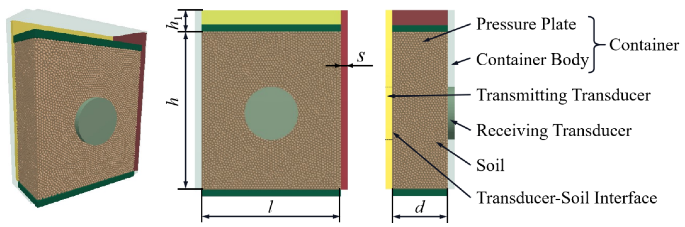
2.1.1. The Geometric Model

The geometric model of the experimental device, which includes the container and ultrasonic transducers, is created using 3D modeling software (SolidWorks 2018), as illustrated in Figure 1. The container is designed to hold soil and securely mount the ultrasonic transducers (comprising both the transmitting transducer and the receiving transducer), which are employed to simulate vibrations in order to generate ultrasonic signals.
The container consists of a container body and a pressure plate. Except for the pressure plate, which can slide up and down along the inner wall of the container body, all other components are fixed in place. An ultrasonic transmitting transducer and a receiving transducer are arranged on opposite sides of the container and positioned coaxially. To simulate soil compaction, we establish a soil compression rate by adding a pressure plate to the top of the container, ensuring that the lower plane of the pressure plate is coplanar with the upper plane of the container body in its initial position. During the experiment, we adjust the sliding distance of the pressure plate according to the required soil compression rate, thereby applying varying degrees of compression to the soil.
The dimensions of the container are as follows: length (l) = 100 mm, height (h) = 130 mm, and width (d) = 40 mm. Both the container body and the pressure plate are constructed from steel plates with a thickness (s) of 10 mm. The height (h1) from the lower plane of the pressure plate to the upper edge of the container body represents the sliding distance of the pressure plate. The soil compression rate is calculated using Equation (1).
α = h 1 / h
where α is the soil compression rate, %. h1 is the height from the lower plane of the pressure plate to the upper edge of the container body, mm. h is the hight of the container, mm.

2.1.2. The Soil Particle Model and Parameters

To investigate propagation laws of ultrasound among soil particles, this article focuses on pure soil as the research object, excluding other substances and moisture. The Hertz–Mindlin model is chosen for modeling due to the relatively weak binding force between dry soil particles. Soil particles are represented as circular particles, and a particle factory is positioned above the container to generate this type of particle. Under the influence of gravity (g = 9.8 m/s2), soil particles fall freely, with a total of 600,000 particles filling the container. To enhance computational efficiency, the particle size of soil particles is scaled up to 2 mm. The material parameters for the model are set as shown in Table 1, and the material contact parameters are specified in Table 2. The particles are dropped into the container to simulate the soil conditions. In order to create optimal ultrasonic propagation conditions, the compression ratio is set to 12%, corresponding to h1 = 15.60 mm. The fixed time step is set to 1.0 × 10⁻⁷ s (2% of the Rayleigh time step), and the grid unit size is established at 2 mm (twice the minimum particle radius). The soil model parameters primarily include physical and contact parameters of soil particles, with the settings for these parameters mainly referring to the research conducted by Ucgul et al. [33,34,35].

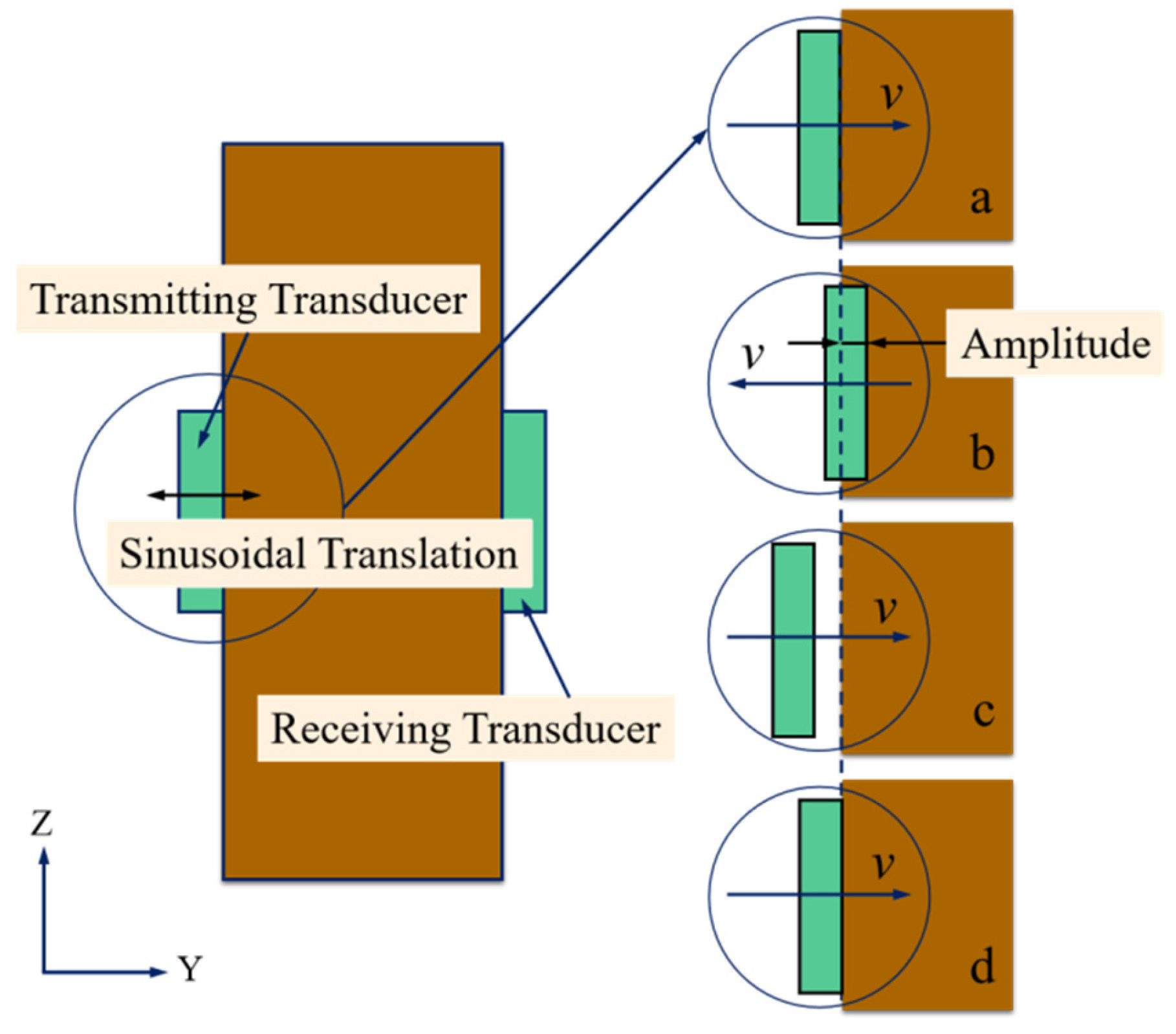
2.1.3. Generation of Ultrasonic Continuous Signals

Sound waves are fundamentally vibrations of the medium through which they propagate, while ultrasonic waves are sound waves with vibration frequencies exceeding 20 kHz. In experiments, ultrasonic continuous signals can be generated using a signal generator, while in simulation, vibration is modeled by applying periodic reciprocating motion to the “transmission transducer model”. The frequency and amplitude of this reciprocating motion correspond to the frequency and amplitude of the simulated vibration.
In this experiment, the motion mode of the transmitting transducer is set to sinusoidal translation. Figure 2 illustrates a schematic diagram of the transmitting transducer motion. When the signal is transmitted, the transmitting transducer begins at its original position and moves in the positive direction of the Y-axis (Figure 2a). Upon reaching the maximum movement distance, the distance from the transmitting transducer to the original position is referred to as the amplitude (Figure 2b). It then starts moving in the negative direction of the Y-axis, and after reaching the farthest point, it reverses direction again to move in the positive direction of the Y-axis (Figure 2c). When it returns to its original position, a complete movement cycle is accomplished (Figure 2d). While transmitting ultrasonic continuous signals, the transmitting transducer does not stop moving as it passes passing through the original position; instead, it continues to repeat the aforementioned motion process according to the set motion frequency within the defined time (Figure 2a–d).

2.2. Characterization of Ultrasonic Signals

2.2.1. Characterization Method before Entering Interface

Before entering the transmitting transducer–soil interface (Figure 1), the generation and transmission process of ultrasonic signals occurs, which exclusively involves the movement of the transmitting transducer itself and does not involve the movement of the soil. Therefore, the movement of the transmitting transducer is utilized to characterize the ultrasonic signal. The methods for generating and transmitting ultrasonic signals have been described in Section 2.1.3.

2.2.2. Characterization after Passing through the Interface

The transmitting transducer is designed to make close contact with the soil in the experimental device. When the transducer begins to reciprocate, the interaction between the transducer and the soil particles facilitates the propagation of ultrasonic signals into the soil particles. Since the interaction between the transmitting transducer and the soil is characterized by “force and reaction force”, this paper studies the force exerted by the transmitting transducer to examine the mechanical characteristics of soil particles at the interface. Considering that the end face area of the transmitting transducer is equivalent to the stress area (S) of the soil at the interface, the pressure (p) is used for convenience instead of the force (F). The conversion formula between pressure and force is provided in Equation (2). In summary, ultrasonic signals are characterized by the pressure applied to the soil particles at the interface.
p = F / S
where p is the pressure applied to the transmitting transducer, Pa. F is the force applied to the transmitting transducer, N. S is the stress area of the transmitting transducer–soil interface, m2.
Because of the weight of soil and the compression of pressure plate, an initial pressure (P0) exists between the soil and the transducer at the start of the experiment. Assuming that when the ultrasonic signal generated by the transducer vibration acts on the soil, the measured pressure is P1, and the interaction pressure |P| between the ultrasonic signal and the soil is given by:
| P | = | P 1 P 0 |
where |P| is the interaction pressure between the ultrasonic signal and the soil, Pa. P1 is the measured pressure when the ultrasonic signal generated by the transducer vibration acts on the soil, Pa. P0 is the pressure between soil and transducer at the initial time of experiment, Pa.

2.3. Experiment Factors and Levels

Excitation frequency and excitation amplitude of ultrasonic signal are two important parameters in ultrasonic detection. The attenuation characteristics of ultrasound waves at different frequencies vary across different materials. Low-frequency signals, although having low axial resolution, are suitable for high-attenuation materials due to relatively weaker attenuation and better penetration capability. In contrast, high-frequency signals offer greater axial resolution and higher detection accuracy but experience more severe attenuation, making them more suitable for low-attenuation materials. Considering that soil is a porous medium with strong attenuation characteristics, the ultrasonic frequency range typically used for detection it is relatively low, generally between 1 kHz and a few tens of kHz. To study the influence of different excitation frequencies on the propagation of ultrasonic continuous signals, the excitation frequency is set as one of the experimental factors. Based on the aforementioned principles and by referencing previous studies, we have set the levels at 20 kHz, 40 kHz, and 60 kHz [36,37,38]. The larger the amplitude of ultrasonic excitation, the greater the energy carried by the signal. A larger excitation amplitude facilitates the distinction of the received signal from noise and other interference signals, making it easier to identify and analyze the received signal. In order to study the influence of different excitation amplitude on the propagation of ultrasonic continuous signals, the excitation amplitude is taken as the second experimental factor, with three levels set at 0.005 mm, 0.010 mm and 0.015 mm. A total of 9 experiments are conducted using a full-factorial design. Detailed parameter settings are presented in Table 3.

2.4. Data Acquisition

The peak value and trough value of ultrasonic signal represent the maximum and minimum values of the interface soil pressure, respectively, indicating the influence range of ultrasonic signal on soil medium and serving as important parameters for ultrasonic signal analysis. It has been observed that the soil pressure itself changes regularly during the transmission of ultrasonic continuous signals. As the excitation frequency and excitation amplitude vary, the peak value and trough values of pressure correlate with these changes. In order to reveal the variation law of soil pressure at the interface under the influence of continuous signals, we select three parameters: the peak value of the first wave (|H0|), the peak value of other waves (|H|) and the trough value (|L|). We analyze their relative values and their variation with excitation frequency and excitation amplitude in detail. In Figure 3, we use the interface soil pressure image with an excitation frequency of 40 kHz and excitation amplitude of 0.010 mm as an example, labeling the key wave bands and important points. We analyze only the wave bands where the signal has been transmitted (“Early wave”, “Wave in the process” and “Late wave”). The “Wave after the transmitting transducer stops moving” is only labeled in Figure 3 and is not analyzed.
Under each detection condition, we extract |H0| and calculate |H| and |L|. We plot images of |H0|, |H| and |L| with respect to frequency and amplitude, and analyze the peak and trough values in relation to frequency and amplitude. The correlation coefficient R between soil pressure and excitation amplitude is calculated using Excel. We also calculate the difference J between the peak values of all waves except for the first wave and trough values under various experimental conditions, and analyze the reasons for its variations as well as the influence of frequency and amplitude.

2.4.1. The Peak Value of the First Wave |H0|

After the continuous ultrasonic signal is transmitted, the waveform formed by the first vibration period is referred to as the first wave. Preliminary experiments have found that the peak value of the first wave (|H0|) is consistently smaller than the peak value of other waves (|H|), and there is a significant difference compared to the peak values of other waves. Therefore, the peak value of the first wave (|H0|) (Figure 3) under each experimental condition is extracted and analyzed separately.

2.4.2. The Peak Value of Other Waves |H|

In order to make the data more generalizable, the peak values of other waves, excluding the first wave, from five cycles starting from the second cycle are selected, and their average values represent the peak values of other waves under this detection condition. |H| is calculated using Equation (4).
| H | = | ( H 1 + H 2 + H 3 + H 4 + H 5 ) / 5 |
where |H| is the peak values of other waves, Pa. H1H5 are the peak values of other waves except the first wave in 5 cycles from the second cycle, Pa.

2.4.3. The Trough Value |L|

Since there is no significant difference between the first trough and other troughs excluding the first wave, we select the trough values |L1|–|L5| (Figure 3) from the first cycle for five consecutive cycles, and their average value represents the trough value of the curve under this detection condition. |L| is calculated using Equation (5).
| L | = | ( L 1 + L 2 + L 3 + L 4 + L 5 ) / 5 |
where |L| is the trough value, Pa. L1L5 are the troughs of 5 consecutive cycles from the trough of the first cycle, Pa.

2.4.4. The Difference J between |H| and |L|

The difference between the peak value of other waves |H| and the trough value |L| is represented by J. J is calculated using Equation (6). The J value is calculated at different excitation frequencies and amplitudes, and an image is plotted showing how the J value changes with the excitation frequency and amplitude.
J = | H | | L |
where J is the difference between |H| and |L|, Pa. |H| is the peak value of other waves, Pa. |L| is the trough value, Pa.

3. Results and Analysis

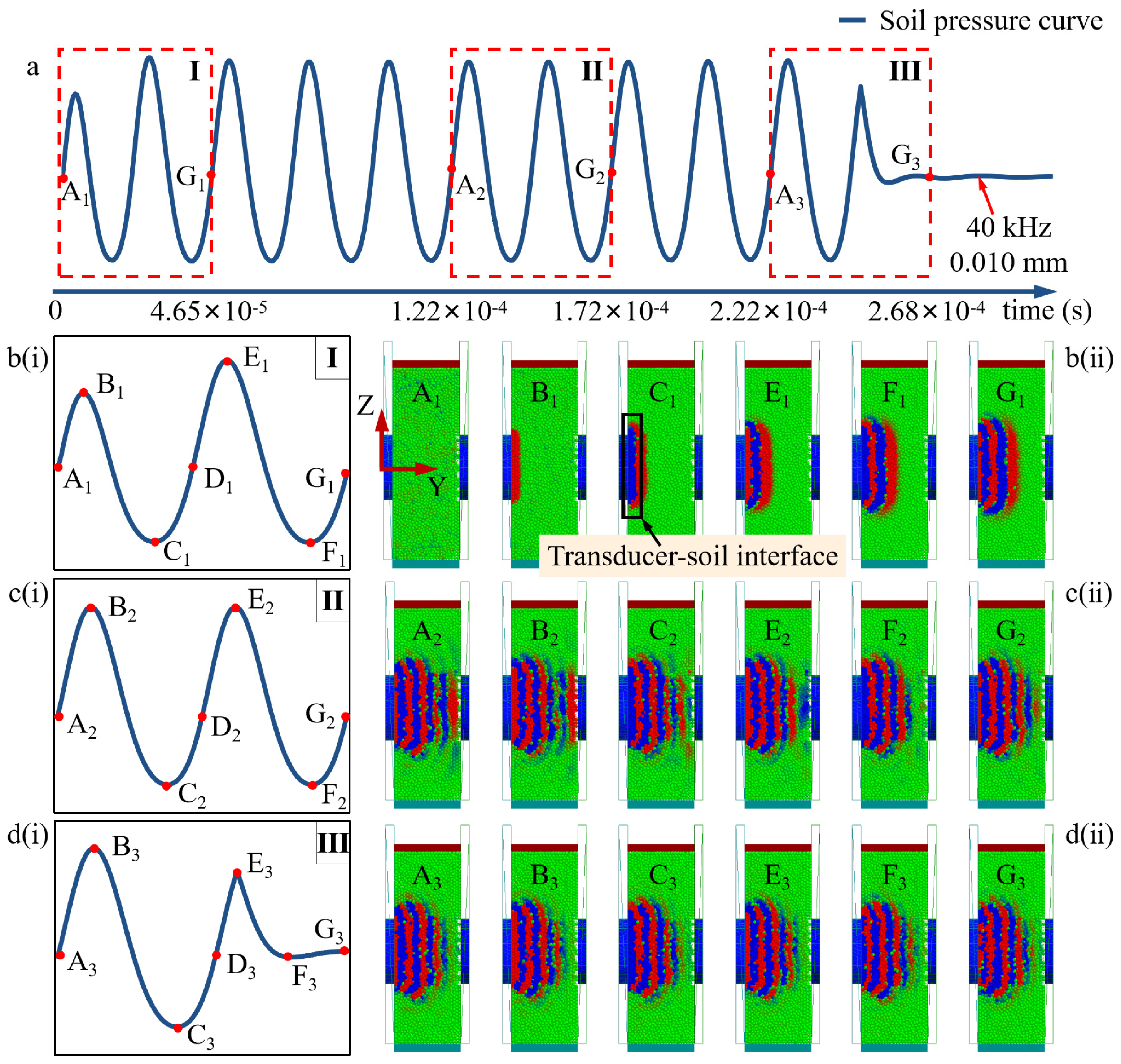
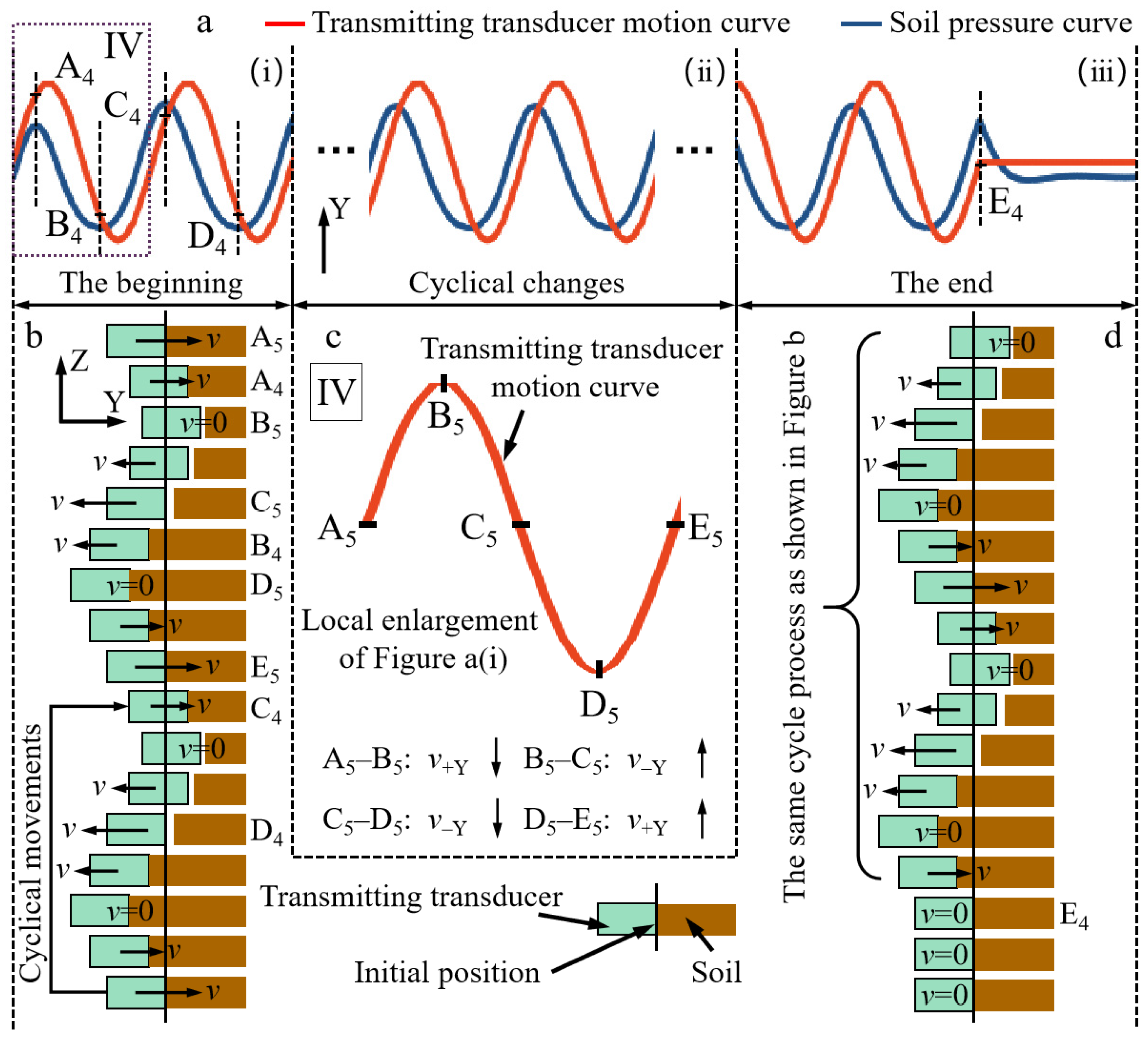
3.1. Analysis of Continuous Ultrasonic Signal Transmitting Process

In order to illustrate the change in soil pressure at the interface from the beginning to the end of the signal transmission (Figure 4), as well as the variation in soil particle pressure near the interface under the continuous action of transmitting transducer (Figure 5), this paper analyzes the key steps during the time period of 0–2.68 × 10⁻⁴ s. The pressure curves of soil and particles at the interface exhibit similar characteristics across each experimental group. Therefore, using an excitation frequency of 40 kHz and an excitation amplitude of 0.010 mm as an example, the transmitting process of ultrasonic continuous signal is analyzed, with the initial signal transmitting time of transmitting transducer set as 0 s.
As shown in Figure 4a, the ultrasonic signal transmission process in the interface soil mainly includes three forms: I, II and III, which correspond to the initial stage of signal transmission, the stabilization of the signal transmission, and the moment just before the signal transmission stops, respectively. Within a continuous section of signal, form I and form III appear only once, while form II appears cyclically between form I and III. The number of occurrences of form II depends on the number of transmission periods set.

3.1.1. The Initial Stage of Signal Transmission

In the initial stage of signal transmission, the soil is stationary (Figure 4(b(i)) A1), while the transmitting transducer has an initial velocity in the positive direction of the Y-axis (Figure 5b,c A5). The interface soil is compressed and the stress gradually increases. The soil particles at the interface are red (Figure 4(b(ii)) A1–B1) and begin to move forward towards the Y-axis.
After the transmission begins, the transmitting transducer decelerates gradually (Figure 5b,c A5–B5), and the soil also decelerates due to internal resistance until the acceleration of the transmitting transducer matches that of the soil (Figure 5(a(i),b) A4), at which point the soil pressure reaches its maximum value (Figure 4(b(i)) B1).
Since then, both the transmitting transducer and the soil continue to move forward to the Y axis, but because the velocity of the transmitting transducer is lower than that of the soil, the transmitting transducer gradually separates from the soil, causing the interface soil pressure to begin decreasing. After that, the forward velocity of the transmitting transducer decreases to 0 (Figure 5b,c B5) and starts to accelerate in the reverse direction (Figure 5b,c B5–C5). During this process, the degree of separation between the transmitting transducer and the interface soil increases, the pressure on the interface soil decreases, and the soil becomes loose gradually. At this point, the soil pressure shifts to the negative direction of Y axis, and the particles turn blue (Figure 4(b(ii)) B1–C1). The soil begins to move in the opposite direction when the velocity decreases to 0.
The transmitting transducer starts to decelerate when it passes through the initial position (Figure 5b,c C5), while the soil accelerates to the negative direction of the Y axis. When the velocity of the interface soil matches that of the transmitting transducer (Figure 5(a(i),b) B4), the interface soil pressure reaches its minimum value (Figure 4(b(i)) C1).
After that, the contact degree between the transmitting transducer and the interface soil increases, causing the interface soil to be compressed again, which leads to an increase in the interface soil pressure. When the velocity of transmitting transducer decreases to 0 (Figure 5b,c D5), it accelerates to Y-axis again (Figure 5b,c D5–E5), and the pressure on soil particles increases continuously. At this time, the interface soil particles are red (Figure 4(b(ii)) C1–E1).

3.1.2. The Stage of Signal Transmission Process

The transmitting transducer starts the movement of the second cycle after completing the first cycle, and the interaction process between the transmitting transducer and the interface soil is the same as in the first cycle. When the acceleration of the transmitting transducer toward the Y-axis matches that of the soil (Figure 5(a(i),b) C4), the soil pressure reaches its maximum value (Figure 4(b(i)) E1), after which the soil pressure begins to decrease. When the velocity of the interface soil equals that of the transmitting transducer (Figure 5(a(i),b) D4), the pressure on the interface soil reaches a minimum (Figure 4(b(i)) F1).
Observing the stress curve of soil at the interface (Figure 4a), it can be seen that the peak value of other waves |H| are larger than the peak value of the first wave |H0|. This may be because the motion of the transmitting transducer has not completed a full cycle when the interface soil pressure curve forms a cycle (Figure 4(b(i)) D1, G1). When the transducer completes a full cycle and returns to the initial position again (Figure 5b,c E5), the interface soil pressure value exceeds the initial pressure value. Therefore, when the transmitting transducer moves from the initial position for the second time, the peak value (Figure 4(b(i)) E1) of the interface soil pressure is larger than that of the first time (Figure 4(b(i)) B1). From the second period of transducer movement, the stress process of the soil interface is the same as that of the second period, so only the peak value of the first wave |H0| is smaller than that of other waves |H|.
Due to the inertia of soil particles, early soil pressure will transmit into the interior of the soil. Therefore, during the signal transmission process, radial red and blue alternating bands (Figure 4(b(ii)) G1) can be observed diffusing into the soil.
During the signal transmission process, the transmitting transducer continuously cycles back and forth. The pressure on the interface soil varies with the movement of the transmitting transducer (Figure 5(a(ii))), showing a consistent variation law in each cycle (Figure 4(c(i)) A2–D2, D2–G2), similar to that in the second cycle of signal transmission (Figure 4(b(i)) D1–G1). In each cycle, the peak value and trough values of the interface soil stress waveform remain consistent.
J is always positive under all detection conditions (the minimum value of J occurs at an excitation frequency of 20 kHz and an excitation amplitude of 0.005 mm, which is 6674.6 Pa, also positive). This may be due to the fact that when the transmitting transducer moves forward toward the Y-axis, the compression degree of the interface soil increases, the range of soil particles to move decreases, and the rate of pressure change is large. However, when the transmitting transducer moves negatively toward Y-axis, the soil becomes loose, the soil rebound speed decreases, and the rate of pressure change decreases. Therefore, the interface soil pressure increases more when the transmitting transducer moves positively toward the Y-axis, and decreases less when it moves negatively toward the Y-axis, which results in an increase in J.
During the signal transmission process, the soil at the interface is continuously subjected to alternating pressure from the transmitting transducer [39]. At this stage, the magnitude and direction of the interface soil pressure are constantly changing, and are continuously transmitted to the interior of the soil, causing the color of particles at the interface and within the soil to alternate between red and blue at each time moment (Figure 4(c(ii)) A2–G2).

3.1.3. The End Stage of Signal Transmission

At the end stage of signal transmission, the transmitting transducer stops at the initial position after completing the last complete movement cycle (Figure 5(a(iii)) E4), after which the transmitting transducer does not move any more (Figure 5d E4). Before the transmitting transducer stops, the pressure curve of the interface soil (Figure 4(d(i)) A3–E3) and the color change in the soil particle pressure (Figure 4(d(ii)) A3–E3) are consistent with the stage of signal transmission process. At the moment the transmitting transducer stops, the interface soil still has a positive velocity towards the Y-axis. At this time, the interface soil gradually separates from the transmitting transducer, the pressure drops sharply, the pressure curve shows a sharp peak (Figure 4d(i) E3), while the color of the interface soil particles is red (Figure 4(d(ii)) E3). The interface soil oscillates several times along the positive and negative directions of Y-axis in situ, and then gradually comes to rest. At this point, the pressure on the interface soil (Figure 4(d(i)) F3–G3) fluctuates several times around the initial value and then returns to the initial value. The color of the interface soil particles begins to trend towards a chaotic state of mixing red and blue (Figure 4(d(i)) G3), and the changes in pressure on the interface soil are no longer regular.
After the transducer stops moving, the red and blue pressure waves generated in the early stage continue to diffuse into the soil (Figure 4(d(ii)) G3), but no new red or blue bands are produced at the interface, marking the end of the signal transmission process.

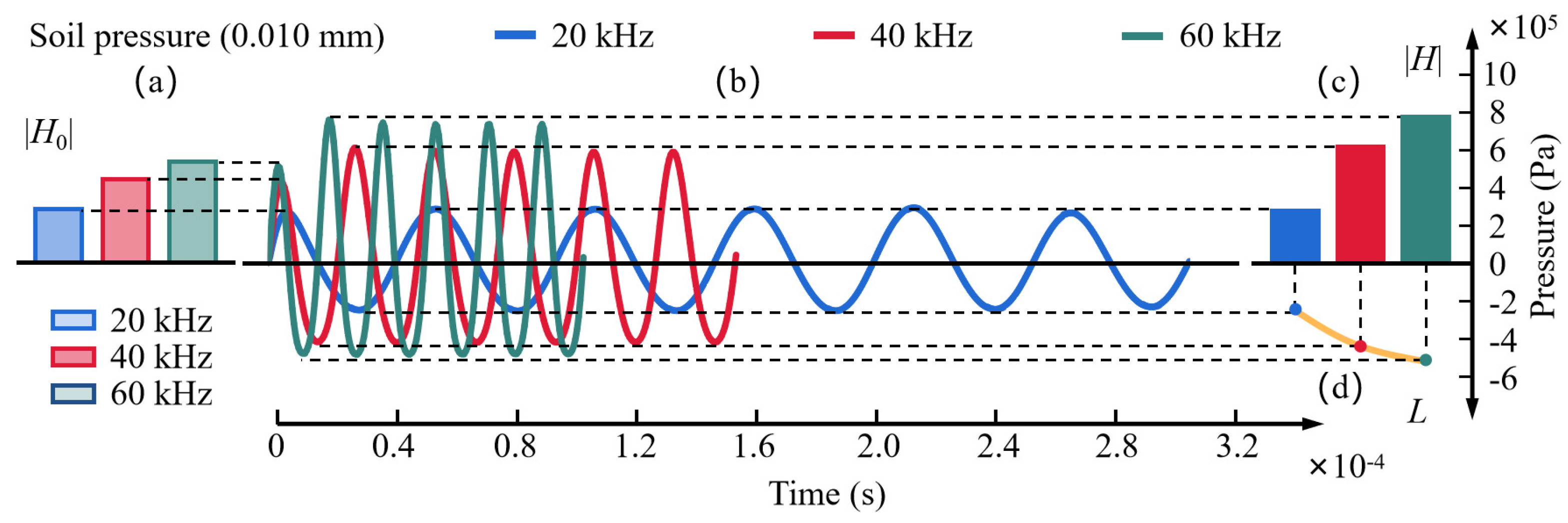
3.2. The Effect of the Excitation Frequency on the Waveform

In order to explore the influence of the excitation frequency on the peak and trough values of the ultrasonic continuous signal, we plot the change curves (Figure 6b) of soil pressure at different excitation frequencies (20 kHz, 40 kHz, and 60 kHz) when the excitation amplitude is 0.010 mm. The |H0| (Figure 6a), |H| (Figure 6c) and |L| (Figure 6d) of the curves are extracted separately for comparative analysis, and the results are as follows.

3.2.1. The Peak Value of the First Wave |H0| and the Peak Value of Other Waves |H|

Observing the pressure waveforms of the interface soil at different excitation frequencies (Figure 6b), it can be seen that |H0| increases with the increase in the excitation frequency. When the excitation frequency is 40 kHz and 60 kHz, |H0| is 158% and 191% of that at 20 kHz, respectively (Figure 6a). |H| also increases with the increase in the excitation frequency. When the excitation frequency is 40 kHz and 60 kHz, |H0| is 210% and 263% of that at 20 kHz, respectively (Figure 6c).
Both |H0| and |H| increase with increasing excitation frequency, likely because a higher frequency results in greater acceleration of the transmitting transducer compared to the soil, allowing the transmitting transducer to exert pressure on the soil for a longer duration. At this time the transmitting transducer is separated from the soil more to the right (Figure 5b A4), leading to a greater peak in interface soil pressure. The study of Yang, Wang, Zhang and Wang [39] also showed that increasing the vibration frequency increases the pressure exerted on the particles, which is consistent with the findings of this paper.

3.2.2. The Trough Value |L|

|L| increases with increasing excitation frequency. When the excitation frequency is 40 kHz and 60 kHz, |L| is 167% and 192% of that at 20 kHz, respectively (Figure 6d). This may be due to the fact that when the excitation frequency increases, the motion velocity of the transmitting transducer increases, leading to a greater separation from the soil. When the separation degree of the transmitting transducer from the interface soil is maximized, the distance of separation is larger and the value of pressure is smaller than when the excitation frequency is low, thus making |L| larger. The study of Gheibi and Hedayat [40] also shows that the transmission amplitude is dependent on the true contact area between the particles. An increase in the contact area between particles leads to an increase in the ultrasonic transmission amplitude. Similarly, when the degree of detachment between the particles increases, their contact area decreases, leading to a decrease in amplitude.

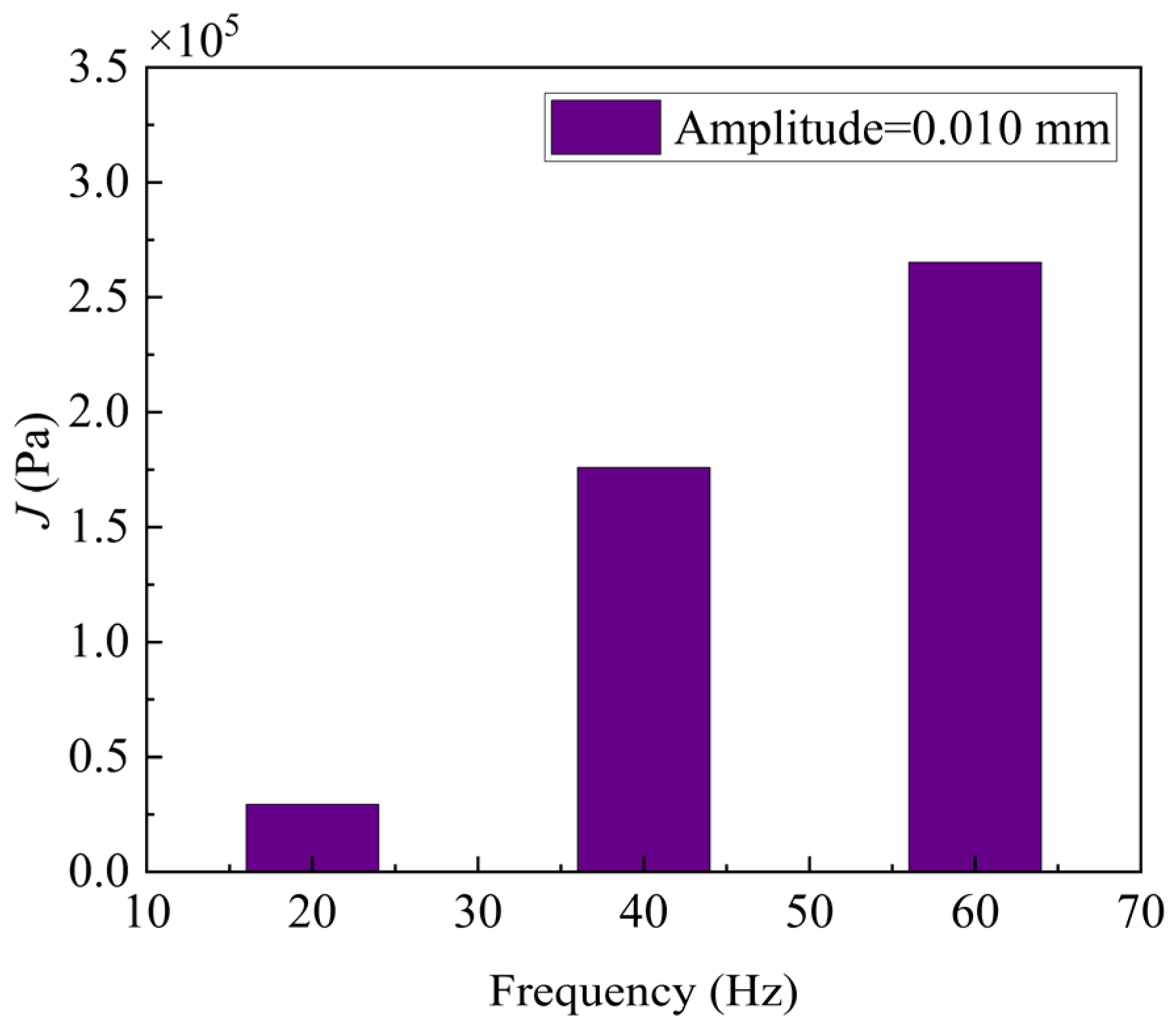
3.2.3. The Difference J between |H| and |L|

J increases with the increase in excitation frequency. When the excitation frequency is 40 kHz and 60 kHz, J is 598% and 900% of that at 20 kHz, respectively (Figure 7). This may be due to the fact that when the transmitting transducer moves positively toward the Y-axis, the squeezing degree of the soil increases, resulting in higher internal stress within the soil. The pressure change becomes more pronounced for the squeezing velocity, i.e., the pressure is more sensitive to the change in squeezing velocity. Therefore, when the interface soil pressure increases, the higher excitation frequency leads to a larger increment in interface soil pressure. When the transmitting transducer moves negatively toward the Y-axis, the extrusion degree of the soil decreases, the soil becomes loose, the soil internal stress decreases, and the sensitivity of the soil pressure to the extrusion velocity decreases. Therefore, when the excitation frequency increases, the decrease in soil pressure |L| (when the soil is squeezed to a lesser extent) is less than the increase in soil pressure |H| (when the soil is squeezed to a greater extent), resulting in an increase in J.

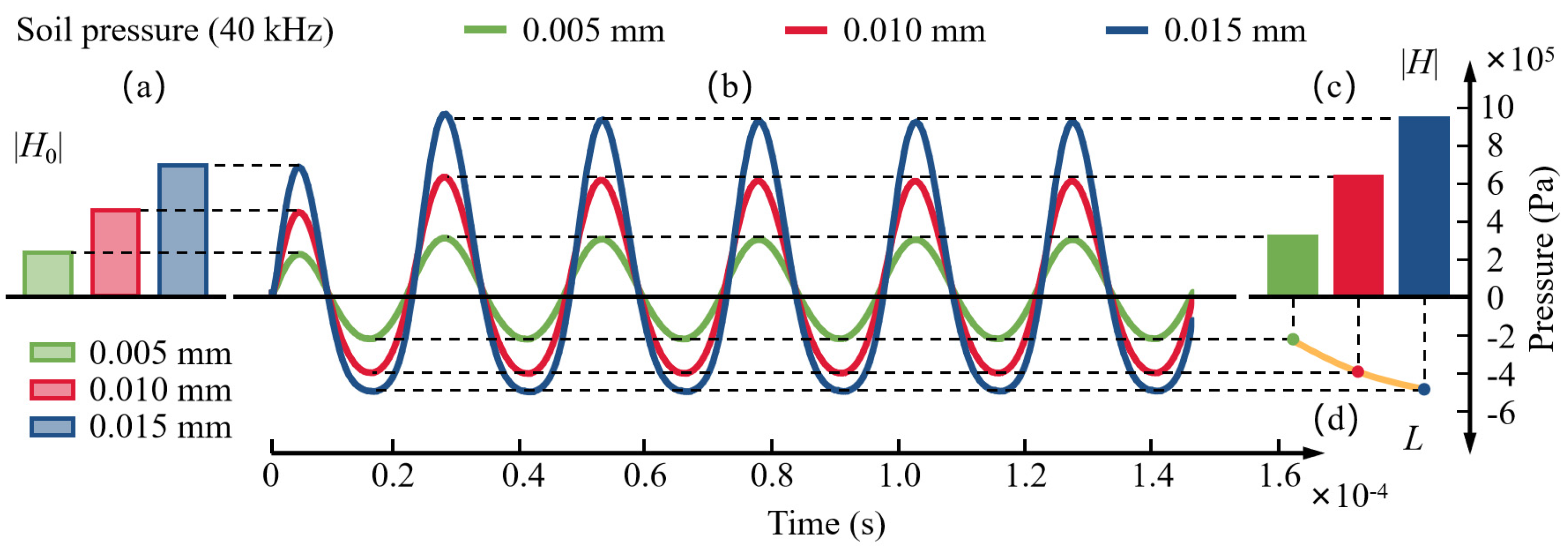
3.3. The Effect of the Excitation Amplitude on the Waveform

In order to explore the influence of the excitation amplitude on the peak and trough values of the ultrasonic continuous signal, we plot the change curves (Figure 8b) of soil pressure at different excitation amplitudes (0.005 mm, 0.010 mm, and 0.015 mm) when the excitation frequency is 40 kHz. The |H0| (Figure 8a), |H| (Figure 8c) and |L| (Figure 8d) of the curves are extracted separately for comparative analysis, and the results are as follows.

3.3.1. The Peak Value of the First Wave |H0| and the Peak Value of Other Waves |H|

Observing the interface soil pressure waveforms at different excitation frequencies (Figure 8b), it can be seen that |H0| increases with the increase in excitation amplitude. When the excitation amplitude is 0.010 mm and 0.015 mm, |H0| is 209% and 327% of that at 0.005 mm, respectively (Figure 8a). This may be due to the increased squeezing of the soil by the transmitting transducer as the excitation amplitude increases. The greater the squeeze the greater the pressure on the soil. |H| also increases with increasing excitation amplitude. When the excitation amplitude is 0.010 mm and 0.015 mm, |H| is 210% and 323% of that at 0.005 mm, respectively (Figure 8c), and the reason for the change in |H| is the same as that of |H0|. The study of Han et al. [41] agrees with the conclusion of this paper that the stress value of the measured object shows an increasing trend as the ultrasonic amplitude increases.
Calculations show that the R-value of |H0| with amplitude is 0.9998, and the R-value of |H| with amplitude is 0.9999, indicating that both |H0| and |H| have a strong positive correlation with the amplitude, and that the mechanical properties of the soil in this state are in accordance with Hooke’s law.

3.3.2. The Trough Value |L|

|L| increases with increasing excitation amplitude. When the excitation amplitude is 0.010 mm versus 0.015 mm, |L| is 174% and 214% of that at 0.005 mm, respectively (Figure 8d). This may be due to the fact that the detachment of the transmitting transducer from the interface soil during its negative movement toward the Y-axis increases with a larger excitation amplitude, leading to a reduction in soil pressure. According to the defining equation of |L|, |L| increases.

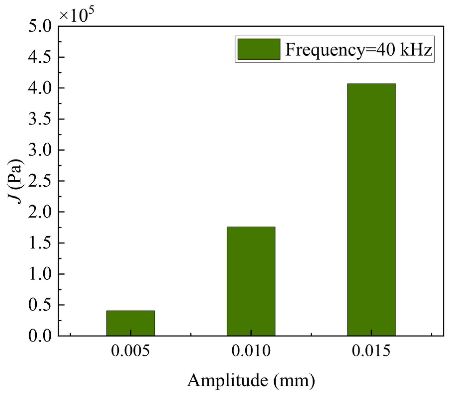
3.3.3. The Difference J between |H| and |L|

J increases with increasing excitation amplitude. When the excitation amplitude is 0.010 mm and 0.015 mm, J is 432% and 1000% of that at 0.005 mm, respectively (Figure 9). This may be due to the fact that the soil is squeezed more when the transmitting transducer is moves towards the Y-axis, which increases the internal stress of the soil, making the pressure change more significant with the change in external squeezing, i.e., the pressure is more sensitive to the change in external squeezing. Therefore, the increase in excitation amplitude leads to a larger increase in soil pressure. Yang, Wang, Zhang and Wang [39] also showed that under ultrasonic vibration, the kinetic energy and stress in the particles increase as the vibration amplitude becomes larger. When the transmitting transducer moves negatively toward the Y-axis, the soil tends to loosen, the internal stress in the soil decreases, and the sensitivity of the soil to changes in squeezing pressure decreases. Therefore, when the excitation amplitude increases, the decrease in soil pressure |L| (when the degree of soil squeezing decreases) is less than the increase in soil pressure |H| (when squeezing the soil), which results in an increase in J.
Taking the curve segment where the peaks H1, H2 and the troughs L2 are located as an example, the images of the peaks and troughs are arranged in the order of increasing excitation frequency and amplitude (Figure 10). In Figure 10, it can be seen that with the increase in the excitation frequency and amplitude, the peaks of the waveforms tend to be sharp while the troughs tend to be flat. This may be due to the fact that as the excitation frequency and amplitude increase, the wave peak values increase more compared to the trough values (i.e., the value of J increases). The larger J is, the more pronounced the phenomenon becomes. It can be observed that although the motion of the transmitting transducer is symmetrical with respect to the initial position, the effect on the soil is mainly generated by inward squeeze. Therefore, in practical application, we should determine the transmitting parameters based on the actual wave peak value to avoid the large inconsistency between the signal amplitude and the design value at the interface soil.

4. Discussion

4.1. Validation of the Reliability of the EDEM Simulation Model

To validate the simulation model used in this study, we conducted verification experiments using an ultrasonic detection platform (Figure 11). The detection platform primarily consists of a signal generator (RIGOL DG1062, RIGOL TECHNOLOGIES Co., Ltd., Beijing, China), an oscilloscope (Tektronix THS3024, Tektronix Inc., OR, USA), a universal material testing machine (RGM-4005, Reger Technologies, Inc., Shenzhen, China), a ultrasonic transmitting transducer (Beijing ZBL Science Technology Co., Ltd., Beijing, China), a ultrasonic receiving transducer (Beijing ZBL Science Technology Co., Ltd., Beijing, China), and a homemade soil ultrasonic detection device.
During the experiment, soil with a diameter of 1–2 mm was screened and dried in an oven until its mass no longer changed. The soil was filled into the homemade soil detection device, and the universal material testing machine was used to compress the soil at the top of the device using a pressure block until the set compression ratio was achieved. The clamping device was then fixed, and ultrasonic detection was performed under the pressure of the pressure plate. An ultrasonic signal was transmitted to the soil via the signal generator and ultrasonic transmitting transducer, and the signal was received and the dominant frequency of the received signal was recorded using the oscilloscope. The excitation frequency, transmission voltage, and compression ratio were set to 20 kHz, 20 Vpp, and 12%, respectively. To measure the frequency of the received signal, we measured the peaks (1st Meas.), troughs (2nd Meas.), and midpoints (3rd Meas.) of the waveforms for two adjacent cycles using the oscilloscope, as well as measuring across the two cycles (4th Meas.). The average of the results from each measurement is presented in Table 4. From the calculated results, it can be seen that the frequency error is less than 0.2%. The experimental results are consistent with the simulation results, with errors within an acceptable range, demonstrating that analyzing ultrasonic waves using the discrete element model is feasible.

4.2. The Potential of This Study in Practical Agricultural Applications

In current agricultural applications, the ultrasonic signals typically used for detection are pulsed signals. However, since the energy intensity of pulsed signals is limited and not entirely suitable for soil detection, we propose using continuous signals with stronger energy. To better serve agricultural applications, we focus on the intermediate wave bands of continuous signals, which have the strongest energy. Additionally, to provide a reference for selecting signal transmission parameters, we studied how the energy of the intermediate wave bands varies with excitation frequency and amplitude.

4.2.1. Advantages of |H|

In addition to the above studies, we also compared the difference between the ultrasonic continuous signal and the pulsed signal. Comparing the waveform of the ultrasonic continuous signal at the ultrasonic transmitting transducer–soil interface (Figure 12a) with the pulsed signal waveform (Figure 12b), it can be found that the first wave of the continuous signal is similar to the first wave of the pulsed signal waveform, and the waveform at the end of the transmission of the continuous signal is also similar to the waveform at the end of the pulsed signal. Therefore, we believe that the pulsed signal is formed by combining the first wave of the continuous signal with the partial waveform at the end of the transmission of the continuous signal, i.e., the ultrasonic pulsed signal waveform is a part of the continuous signal.
The analysis of the ultrasonic continuous propagation process signal in Section 3.1 shows that, although the pressure of the ultrasonic transmitting transducer on the soil varies in the same way in each cycle, the first wave of the signal is different from the other waves (Figure 12a), and the waveform becomes consistent from the second cycle. This indicates that the pressure change at the generation time of the first wave is not yet stable, and the waveform after the second cycle is the result of the stable interaction between the ultrasonic transmitting transducer and the interface soil. Therefore, the intermediate wave band contained in the ultrasonic continuous signal is more stable than the pulsed signal, and the use of the ultrasonic continuous signal can weaken the poor signal transmission caused by poor contact between the ultrasonic transmitting transducer and the interface soil when the signal first contacts the interface soil, making the signal more reliable.
Observing the waveform characteristics of the signal, the wave trough in the middle band of the continuous signal (Figure 12a) is consistent with that of the pulsed signal (Figure 12b), but the wave peak of the continuous signal is larger, about 140% of the pulsed signal. This indicates that the energy of continuous signals is stronger than that of pulsed signals, making them more advantageous in soil media where signal energy attenuation is severe, and thus more suitable for soil detection environments. In summary, the |H| in the continuous signal are more suitable for soil detection environments.

4.2.2. Role of Excitation Frequency and Amplitude

The experimental results in this paper indicate that when the excitation frequency is 40 kHz and 60 kHz, the peak value of the first wave |H0| is 158% and 191% of that at 20 kHz. The peak value of other waves |H| is 210% and 263% of that at 20 kHz, and the trough value |L| is 167% and 192% of that at 20 kHz, respectively. This demonstrates that the energy of the ultrasonic continuous signal increases with an increase in excitation frequency. When the excitation amplitude is 0.010 mm and 0.015 mm, the peak value of the first wave |H0| is 209% and 327% of that at 0.005 mm, and the peak value of other waves |H| is 210% and 323% of that at 0.005 mm, while the trough value |L| is 174% and 214% of that at 0.005 mm, respectively. This indicates that the energy of the ultrasonic continuous signal also increases with the increase in the excitation amplitude. Comparing the influence of excitation frequency and excitation amplitude on signal energy, it can be seen that the signal energy amplification after increasing the excitation amplitude is 1 and 2 times greater than that when the excitation frequency is increased by the same amounts. This shows that the influence of excitation amplitude on signal energy is greater than that of excitation frequency. Due to the significant attenuation in the soil detection environment, we aim to enhance the energy of the transmitting signal as much as possible to facilitate the reception and analysis of the signal. Therefore, when selecting the parameters of the transmitting signal, we should aim to increase both the excitation frequency and amplitude to boost the signal energy, prioritizing the increase in the excitation amplitude in the cases of limited available energy to achieve greater signal energy. In addition, as shown in Figure 10, the excitation frequency and excitation amplitude have different effects on the wave trough, which directly influences the waveform. Understanding the impact of these experimental factors on the waveform itself can allow for a more accurate assessment of the soil’s effect on the waveform.

5. Conclusions

In this paper, we have conducted a preliminary study on the propagation laws of ultrasonic continuous signals in soil. Specifically, we investigated the propagation process of ultrasonic continuous signals at the transducer–soil interface and the variation under different excitation frequencies and amplitudes. For example, the motion curve of the transmitting transducer lags behind the soil pressure changes, and the energy of the ultrasonic signal increases with higher excitation frequency and amplitude. Specifically, |H0| at 40 kHz and 60 kHz is 210% and 263% of that at 20 kHz, respectively. When the excitation amplitude increases from 0.005 mm to 0.015 mm, the value of |H| increases by 323%, among other findings. This provides a foundation for using continuous signals for ultrasonic soil detection.
However, the actual soil environment in the field is highly complex. As a preliminary study of ultrasonic continuous signals, this paper focuses on the propagation mechanism of the signals in soil. Therefore, the experiments were conducted under relatively ideal conditions, with the research subject being uniform and dry soil, without investigating the effects of moisture. Additionally, interference from objects such as stones and plants was not considered. This study also does not explore different soil textures and their varying physical and chemical properties. These factors could potentially impact the results and need to be investigated in future research.
In subsequent studies, we not only need to examine the effects of complex field factors on the signals but also progressively uncover the laws present in the later stages of continuous signal propagation in soil. This will involve studying the complete mechanism of signal propagation in soil to provide theoretical support for the development of ultrasonic soil property detection instruments.

Author Contributions

Z.W., conceptualization, methodology, software, investigation, and writing—review and editing. C.L., project administration, funding acquisition, conceptualization, methodology, and supervision. H.L., funding acquisition and supervision. C.W., supervision. L.W., software and data curation. H.Y., software and data curation. All authors have read and agreed to the published version of the manuscript.

Funding

This work was funded by the National Key Research and Development Program of China (Grant No. 2023YFD1500401), the Program for China Agriculture Research System of MOF and MARA (CARS-03) and the 2115 Talent Development Program of China Agricultural University (2115). Gratitude should be expressed to all the members of Conservation Tillage Research Centre.

Institutional Review Board Statement

Not applicable.

Data Availability Statement

Data are contained within this article. (The original contributions presented in this study are included in this article. Further inquiries can be directed to the corresponding author).

Conflicts of Interest

The authors declare that they have no known competing financial interests or personal relationships that could have appeared to influence the work reported in this paper.

References

  1. Chen, B.B.; Wang, C.; Wang, P.F.; Zheng, S.L.; Sun, W.M. Research on Fatigue Damage in High-Strength Steel (FV520B) Using Nonlinear Ultrasonic Testing. Shock Vib. 2020, 2020, 15. [Google Scholar] [CrossRef]
  2. Beamish, S.; Reddyhoff, T.; Hunter, A.; Dwyer-Joyce, R.S. A method to determine acoustic properties of solids and its application to measuring oil film thickness in bearing shells of unknown composition. Measurement 2022, 195, 111176. [Google Scholar] [CrossRef]
  3. Hussin, M.; Chan, T.H.T.; Fawzia, S.; Ghasemi, N. Identifying the Prestress Force in Prestressed Concrete Bridges Using Ultrasonic Technology. Int. J. Struct. Stab. Dyn. 2020, 20, 25. [Google Scholar] [CrossRef]
  4. Secanellas, S.A.; Gallego, J.C.L.; Catalán, G.A.; Navarro, R.M.; Heras, J.O.; Izquierdo, M.A.G.; Hernández, M.G.; Velayos, J.J.A. An Ultrasonic Tomography System for the Inspection of Columns in Architectural Heritage. Sensors 2022, 22, 6646. [Google Scholar] [CrossRef] [PubMed]
  5. Zielinska, M.; Rucka, M. Assessment of Wooden Beams from Historical Buildings Using Ultrasonic Transmission Tomography. Int. J. Archit. Herit. 2023, 17, 249–261. [Google Scholar] [CrossRef]
  6. Di Battista, A.; Price, A.; Malkin, R.; Drinkwater, B.W.; Kuberka, P.; Jarrold, C. The effects of high-intensity 40 kHz ultrasound on cognitive function. Appl. Acoust. 2022, 200, 109051. [Google Scholar] [CrossRef]
  7. Yan, X.L.; Dong, S.Y.; Xu, B.S.; Cao, Y. Progress and Challenges of Ultrasonic Testing for Stress in Remanufacturing Laser Cladding Coating. Materials 2018, 11, 293. [Google Scholar] [CrossRef]
  8. Li, W.; Ma, H.L.; He, R.H.; Ren, X.F.; Zhou, C.N. Prospects and application of ultrasound and magnetic fields in the fermentation of rare edible fungi. Ultrason. Sonochem. 2021, 76, 105613. [Google Scholar] [CrossRef]
  9. Danielak, M.; Przybyl, K.; Koszela, K. The Need for Machines for the Nondestructive Quality Assessment of Potatoes with the Use of Artificial Intelligence Methods and Imaging Techniques. Sensors 2023, 23, 1787. [Google Scholar] [CrossRef]
  10. Schmitz, A.; Badgujar, C.; Mansur, H.; Flippo, D.; McCornack, B.; Sharda, A. Design of a Reconfigurable Crop Scouting Vehicle for Row Crop Navigation: A Proof-of-Concept Study. Sensors 2022, 22, 6203. [Google Scholar] [CrossRef]
  11. Shimizu, H.; Sato, T. Development of strawberry pollination system using ultrasonic radiation pressure. In Proceedings of the 6th International-Federation-of-Automatic-Control (IFAC) Conference on Bio-Robotics (BIOROBOTICS), Beijing, China, 13–15 July 2018; Elsevier: Beijing, China, 2018; pp. 57–60. [Google Scholar] [CrossRef]
  12. Mizrach, A. Determination of avocado and mango fruit properties by ultrasonic technique. Ultrasonics 2000, 38, 717–722. [Google Scholar] [CrossRef]
  13. Ag, M.R.; Mawandha, H.G.; Huda, M.W.N.; Ngadisih, N. The utilization of Sentinel-1 soil moisture satellite imagery for runoff coefficient analysis. IOP Conf. Ser. Earth Environ. Sci. 2022, 1116, 012017. [Google Scholar] [CrossRef]
  14. Bryk, M.; Kolodziej, B. Pedotransfer Functions for Estimating Soil Bulk Density Using Image Analysis of Soil Structure. Sensors 2023, 23, 1852. [Google Scholar] [CrossRef]
  15. Li, J.Z.; Sun, S.L.; Sun, C.R.; Liu, C.; Tang, W.G.; Wang, H.B. Analysis of Effect of Grouser Height on Tractive Performance of Tracked Vehicle under Different Moisture Contents in Paddy Soil. Agriculture 2022, 12, 1581. [Google Scholar] [CrossRef]
  16. Starovoitova, O.A.; Starovoitov, V.I.; Manokhina, A.A.; Voronov, N.V. Methodological Approaches to Constructing 3D Models of Soil in Potato Farming. In Proceedings of the International Conference on World Technological Trends in Agribusiness (WTTA), Omsk, Russia, 4–5 July 2020; IOP Publishing Ltd.: Omsk, Russia, 2020. [Google Scholar] [CrossRef]
  17. Stolt, M.H.; O’Geen, A.T.; Beaudette, D.E.; Drohan, P.J.; Galbraith, J.M.; Lindbo, D.L.; Monger, H.C.; Needelman, B.A.; Ransom, M.D.; Rabenhorst, M.C.; et al. Changing the hierarchical placement of soil moisture regimes in Soil Taxonomy. Soil Sci. Soc. Am. J. 2021, 85, 488–500. [Google Scholar] [CrossRef]
  18. Baskota, A.; Kuo, J.; Lal, A. Gigahertz Ultrasonic Multi-Imaging of Soil Temperature, Morphology, Moisture, and Nematodes. In Proceedings of the 35th IEEE International Conference on Micro Electro Mechanical Systems Conference (IEEE MEMS), Tokyo, Japan, 9–13 January 2022; IEEE: Tokyo, Japan, 2022; pp. 519–522. [Google Scholar] [CrossRef]
  19. Zhang, J.W.; Murton, J.; Liu, S.J.; Sui, L.L.; Zhang, S. Detection of the freezing state and frozen section thickness of fine sand by ultrasonic testing. Permafr. Periglac. Process. 2021, 32, 76–91. [Google Scholar] [CrossRef]
  20. Zhang, Y.M.; Yang, G.; Chen, W.W.; Sun, L.Z. Relation between Microstructures and Macroscopic Mechanical Properties of Earthen-Site Soils. Materials 2022, 15, 23. [Google Scholar] [CrossRef]
  21. Zhao, Z.; Ma, K.; Luo, Y. Application of Ultrasonic Pulse Velocity Test in the Detection of Hard Foreign Object in Farmland Soil. In Proceedings of the 2019 IEEE 4th Advanced Information Technology, Electronic and Automation Control Conference (IAEAC), Chengdu, China, 20–22 December 2019; pp. 1311–1315. [Google Scholar] [CrossRef]
  22. Asteris, P.G.; Mokos, V.G. Concrete compressive strength using artificial neural networks. Neural Comput. Appl. 2020, 32, 11807–11826. [Google Scholar] [CrossRef]
  23. Zeng, Y.Q.; Liu, Q.H. Acoustic detection of buried objects in 3-D fluid saturated porous media: Numerical modeling. IEEE Trans. Geosci. Remote Sens. 2001, 39, 1165–1173. [Google Scholar] [CrossRef]
  24. Bakhtiari-Nejad, M.; Hajj, M.R.; Shahab, S. Dynamics of acoustic impedance matching layers in contactless ultrasonic power transfer systems. Smart Mater. Struct. 2020, 29, 035037. [Google Scholar] [CrossRef]
  25. Wu, J.F.; Zhao, S.X.; Zhang, J.W.; Wang, R.H. A continuous phase-frequency modulation technique and adaptive pump noise cancellation method of continuous-wave signal over mud telemetry channel. Digit. Signal Prog. 2021, 117, 103147. [Google Scholar] [CrossRef]
  26. Cho, S.; Jeon, K.; Kim, C.W. Vibration analysis of electric motors considering rotating rotor structure using flexible multibody dynamics-electromagnetic-structural vibration coupled analysis. J. Comput. Des. Eng. 2023, 10, 578–588. [Google Scholar] [CrossRef]
  27. Shen, H.M.; Li, X.Y.; Li, Q.; Wang, H.B. A method to model the effect of pre-existing cracks on P-wave velocity in rocks. J. Rock Mech. Geotech. Eng. 2020, 12, 493–506. [Google Scholar] [CrossRef]
  28. Yan, D.X.; Yu, J.Q.; Wang, Y.; Zhou, L.; Sun, K.; Tian, Y. A Review of the Application of Discrete Element Method in Agricultural Engineering: A Case Study of Soybean. Processes 2022, 10, 1305. [Google Scholar] [CrossRef]
  29. Zhao, H.B.; Huang, Y.X.; Liu, Z.D.; Liu, W.Z.; Zheng, Z.Q. Applications of Discrete Element Method in the Research of Agricultural Machinery: A Review. Agriculture 2021, 11, 425. [Google Scholar] [CrossRef]
  30. Xu, L.F.; Feng, T.T.; Song, Y.P.; Li, F.D.; Song, Z.H. Research on Drag Reduction Mechanism of Bionic Rib Subsoiling Shovel Based on Discrete Element Method. In Proceedings of the 3rd International Workshop on Renewable Energy and Development (IWRED), Guangzhou, China, 8–10 March 2019; IOP Publishing Ltd.: Guangzhou, China, 2019. [Google Scholar] [CrossRef]
  31. Yang, L.W.; Chen, L.S.; Zhang, J.Y.; Liu, H.J.; Sun, Z.C.; Sun, H.; Zheng, L.H. Fertilizer sowing simulation of a variable-rate fertilizer applicator based on EDEM. In Proceedings of the 6th International-Federation-of-Automatic-Control (IFAC) Conference on Bio-Robotics (BIOROBOTICS), Beijing, China, 13–15 July 2018; Elsevier: Beijing, China, 2018; pp. 418–423. [Google Scholar] [CrossRef]
  32. Zhou, W.Q.; Ni, X.; Song, K.; Wen, N.; Wang, J.W.; Fu, Q.; Na, M.J.; Tang, H.; Wang, Q. Bionic Optimization Design and Discrete Element Experimental Design of Carrot Combine Harvester Ripping Shovel. Processes 2023, 11, 1526. [Google Scholar] [CrossRef]
  33. Huang, S.H.; Lu, C.Y.; Li, H.W.; He, J.; Wang, Q.J.; Yuan, P.P.; Gao, Z.; Wang, Y.B. Transmission rules of ultrasonic at the contact interface between soil medium in farmland and ultrasonic excitation transducer. Comput. Electron. Agric. 2021, 190, 106477. [Google Scholar] [CrossRef]
  34. Ucgul, M.; Saunders, C.; Fielke, J.M. Discrete element modelling of tillage forces and soil movement of a one-third scale mouldboard plough. Biosyst. Eng. 2017, 155, 44–54. [Google Scholar] [CrossRef]
  35. Ucgul, M.; Fielke, J.M.; Saunders, C. 3D DEM tillage simulation: Validation of a hysteretic spring (plastic) contact model for a sweep tool operating in a cohesionless soil. Soil Tillage Res. 2014, 144, 220–227. [Google Scholar] [CrossRef]
  36. Sarro, W.S.; Assis, G.M.; Ferreira, G.C.S. Experimental investigation of the UPV wavelength in compacted soil. Constr. Build. Mater. 2021, 272, 121834. [Google Scholar] [CrossRef]
  37. Ferreira, C.; Rios, S.; Cristelo, N.; Viana da Fonseca, A. Evolution of the optimum ultrasonic testing frequency of alkali-activated soil–ash. Géotech. Lett. 2021, 11, 158–163. [Google Scholar] [CrossRef]
  38. Tanaka, K.; Suda, T.; Hirai, K.; Sako, K.; Fukagawa, R. Monitoring of Soil Moisture and Groundwater Level Using Ultrasonic Waves to Predict Slope Failures. Jpn. J. Appl. Phys. 2009, 48, 09KD12. [Google Scholar] [CrossRef]
  39. Yang, Z.B.; Wang, X.F.; Zhang, L.; Wang, J.Y. Research on influencing factors of rock breaking efficiency under ultrasonic vibration excitation. AIP Adv. 2023, 13, 13. [Google Scholar] [CrossRef]
  40. Gheibi, A.; Hedayat, A. Ultrasonic investigation of granular materials subjected to compression and crushing. Ultrasonics 2018, 87, 112–125. [Google Scholar] [CrossRef]
  41. Han, J.P.; Zhao, D.J.; Zhang, S.L.; Zhou, Y. Damage Evolution of Granite under Ultrasonic Vibration with Different Amplitudes. Shock Vib. 2022, 2022, 14. [Google Scholar] [CrossRef]
Figure 1. The geometric model of the experimental device, including the container and ultrasonic transducers. The dimensions of the container are as follows: length (l) = 100 mm, height (h) = 130 mm, and width (d) = 40 mm. The container body and the pressure plate are made of steel plates with a thickness (s) of 10 mm. The container is designed to hold soil and secure the ultrasonic transducers (including both the the transmitting and receiving transducers), which are utilized for simulating vibrations to generate ultrasonic signals. A total of 600,000 soil particles are allowed to free-fall into the container under the influence of gravity (g = 9.8 m/s2), using the Hertz–Mindlin model with an expanded particle size of 2 mm. The upper pressure plate is pressed down h1 along the inner wall of the container to achieve a set soil compression rate of 12%. The fixed time step is set to 1.0 × 10⁻⁷ s (2% of the Rayleigh time step), and the grid unit size is set to 2 mm (twice the minimum particle radius).
Agriculture 14 01470 g001
Figure 2. Schematic diagram of the transmitting transducer motion. The motion mode of the transmitting transducer is set to sinusoidal translation. When transmitting an ultrasonic signal, the transmitting transducer actively translates along the Y axis, while the receiving transducer remains stationary. When the signal is transmitted, the transmitting transducer starts from its original position and moves in the positive direction of the Y-axis (a). Upon reaching the maximum movement distance, the distance from the transmitting transducer to its original position is defined as the amplitude (b). It then begins to move in the negative direction of the Y-axis, and after reaching the farthest position, it reverses direction again to move in the positive direction of the Y-axis (c). When it returns to its original position, it completes a full movement cycle (d). During the transmission of ultrasonic continuous signals, the transmitting transducer does not stop moving when passing through the original position, but continues to repeat the above motion process according to the set motion frequency within the defined time (ad).
Agriculture 14 01470 g002
Figure 3. Interface soil pressure waveform at an excitation frequency of 40 kHz and an excitation amplitude of 0.010 mm. The signal is received at 0 s, and the soil pressure changes in the time period of 0–5 × 10⁻⁴ s are observed, including the 10-cycle ultrasonic signal when the transmitting transducer is moving and the soil pressure change after the transmitting transducer stops moving. Based on the characteristics of the waveform, the entire waveform is divided into four bands: “Early wave”, “Wave in the process”, “Late wave” and “Wave after the transmitting transducer stops moving”. In the subsequent analysis, only the bands in the transmission process (“First wave”, “Wave in the process”, “Late wave”) are analyzed, while the bands after the transmission stops is only labeled and not analyzed. H0–H5 represent the peak positions of the first six cycles, and L1–L5 represent the trough positions of the first five cycles. |H1|–|H5| represent the peak value of the wave corresponding to H1–H5 (calculated by Equation (3)), and |L1|–|L5| represent the trough values corresponding to L1–L5 (calculated by Equation (3)). |H0| represents the peak value of the first wave (calculated by Equation (3)), |H| represents the average peak value of other waves (calculated by Equation (4)), and |L| represents the average of the trough values (calculated by Equation (5)). In Equation (3), to distinguish between the peak value and the trough value, when referring to the peak value, |P| = |H| or |P| = |Hx| (x = 0, 1, 2, 3, 4, 5); when referring to the trough value, |P| = |L| or |P| = |Lx| (x = 0, 1, 2, 3, 4, 5).
Agriculture 14 01470 g003
Figure 4. Ultrasonic continuous signal transmitting process (40 kHz-0.010 mm). (a) The complete waveform of the ultrasonic continuous signal at the transmitting transducer–soil interface is labeled with three typical patterns of the ultrasonic transmitting process: I, II, III. I represents the waveform at the initial stage of signal transmission (b(i)), marking the inflection point of the soil pressure change (A1–G1). II is the waveform of the signal transmission process (c(i)), marking the inflection point of the soil pressure change (A2–G2). III is the waveform at the end of the signal transmission (d(i)), which marks the inflection point of the soil pressure change (A3–G3). b(ii), c(ii) and d(ii) show the color changes in soil particles near the interface at the initial stage of signal transmission, during signal transmission process, and at the end of the signal transmission, respectively. The red color of the interface soil particles indicates that the interface soil is compressed, and the soil pressure is in the positive direction of the Y-axis; the blue color of the particles indicates that the interface soil is gradually loosening, and the soil pressure changes to the negative direction of the Y-axis. The same symbol labels in the diagram represent the same meaning or stage.
Agriculture 14 01470 g004
Figure 5. The correspondence between the change in interface soil pressure and the motion of the transmitting transducer. (c) The local enlargement of (a(i)). The motion curve of the transmitting transducer lags behind the soil pressure curve. The change in soil pressure and the motion of the transmitting transducer are divided into three phases: “The beginning” (a(i)), “Cyclical changes” (a(ii)), and “The end” (a(iii)). The blue curve indicates the change in soil pressure, while the red curve indicates the motion trajectory of the transmitting transducer. A4–D4 represent the position of the transmitting transducer when the soil pressure reaches its peak and trough (a(i)), and A5–E5 represent the inflection points where the magnitude and direction of the transmitting transducer’s velocity change (c). (b) shows the changes in the magnitude and direction of the transmitting transducer’s velocity during “The beginning” and “Cyclical changes”, with the meanings of A4–D4, and A5–E5 corresponding to those in (a(i),c). (d) illustrates the motion state during “The end” and after the transmitting transducer stops moving. The length of the arrow indicates the magnitude of the velocity value (b,d). The graph only expresses the correspondence between the soil pressure curve and the motion curve of the transmitting transducer on the time axis, and the magnitude of the curve shape does not represent the actual values.
Agriculture 14 01470 g005
Figure 6. The change curves of soil pressure at different excitation frequencies (20 kHz, 40 kHz, and 60 kHz) when the excitation amplitude is 0.010 mm (b). (a) |H0|, (c) |H| and (d) |L| of the curves are extracted separately for comparative analysis, showing that the |H0|, |H| and |L| increase with the increase in excitation frequency. In (d), ‘L’ is the original value of the trough, which is negative, and it is analyzed in the text according to Equation (5) to become an absolute value |L|.
Agriculture 14 01470 g006
Figure 7. The variation in J with different excitation frequencies (20 kHz, 40 kHz, and 60 kHz) at an excitation amplitude of 0.010 mm, showing that J increases with the increase in the excitation frequency.
Agriculture 14 01470 g007
Figure 8. The change curves of soil pressure at different excitation amplitudes (0.005 mm, 0.010 mm, and 0.015 mm) when the excitation frequency is 40 kHz (b). (a) |H0|, (c) |H| and (d) |L| of the curves are extracted separately for comparative analysis, showing that |H0|, |H| and |L| increase with the increase in excitation amplitude. The R-value of |H0| with amplitude is 0.9998 and the R-value of |H| with amplitude is 0.9999, indicating that both |H0| and |H| have a strong positive correlation with the amplitude. In (d), ‘L’ is the original value of the trough, which is negative, and it is analyzed in the text according to Equation (5) to become an absolute value |L|.
Agriculture 14 01470 g008
Figure 9. The variation in J with different excitation amplitudes (0.005 mm,0.010 mm, and 0.015 mm) at an excitation frequency of 40 kHz, showing that J increases with the increase in the excitation amplitude.
Agriculture 14 01470 g009
Figure 10. As the excitation frequency and amplitude increase, the wave peak values increase more compared to the trough values (i.e., the value of J increases). The larger J is, the more pronounced the phenomenon becomes.
Agriculture 14 01470 g010
Figure 11. Ultrasonic detection platform.
Agriculture 14 01470 g011
Figure 12. Waveform comparison of ultrasonic continuous signal and pulsed signal. (a) Ultrasonic continuous signal waveform. (b) Pulsed signal waveform. The first wave of the continuous signal is similar to that of the pulsed signal waveform, and the waveform at the end of the transmission of the continuous signal is also similar to that of the pulsed signal. Therefore, we believe that the pulsed signal is formed by combining the first wave of the continuous signal with the partial waveform at the end of the transmission of the continuous signal, i.e., the ultrasonic pulsed signal waveform is a part of the continuous signal.
Agriculture 14 01470 g012
Table 1. Model material parameters.
ObjectSoilSteelPzt
Poisson’s Ratio0.300.250.32
Density (kg/m3)265078607900
Shear Modulus (Pa)1.2 × 1097.9 × 10107.5 × 1010
Note: Pzt is the piezoelectric material of the ultrasonic transducer, which represents the surface of the transmitting transducer in contact with the soil in Table 1 and Table 2.
Table 2. Contact parameters.
ObjectSoil-SoilSoil-SteelSoil-Pzt
Coefficient of Restitution0.60.50.5
Coefficient of Static Friction0.50.50.4
Coefficient of Rolling Friction0.160.050.04
Table 3. Experiment factors and levels.
FactorLevel 1Level 2Level 3
Frequency (kHz)204060
Amplitude (mm)0.0050.0100.015
Table 4. Experimental verification results.
ObjectDominant Frequency
Simulation result (kHz)Fourier analysis result
20
Experiment result (kHz)1st Meas.2nd Meas.3rd Meas.4th Meas.Average
20.1619.8420.1610.0020.04
Error (%)0.2
Disclaimer/Publisher’s Note: The statements, opinions and data contained in all publications are solely those of the individual author(s) and contributor(s) and not of MDPI and/or the editor(s). MDPI and/or the editor(s) disclaim responsibility for any injury to people or property resulting from any ideas, methods, instructions or products referred to in the content.

