A Standardized Treatment Model for Head Loss of Farmland Filters Based on Interaction Factors

Abstract

A head loss model for pressureless mesh filters used in farmland irrigation was developed by integrating the four basic test factors: irrigation flow, filter cartridge speed, self-cleaning flow, and initial sand content. The model’s coefficient of determination was found to be 98.61%. Among the basic factors, the total irrigation flow accounted for only 17.20% of the relatively small self-cleaning flow. The contribution of initial sand content was found to be the smallest, with a coefficient of only 0.0166. Furthermore, the contribution rate of the flow term was significantly higher than that of the initial sand content, with a value of 159.73%. In terms of quadratic interaction, the difference between the interaction term of flushing flow and filter cartridge speed, and the interaction term of filter cartridge speed and self-cleaning flow was 38.42%. On the other hand, the difference within this level for the interaction term between initial sand content and filter cartridge speed, as well as the interaction term between irrigation flow and self-cleaning flow, was 2.82%. Finally, through joint optimization of the response surface and model, the optimal values for the irrigation flow rate, filter cartridge speed, self-cleaning flow rate, and initial sand content were determined to be 121.687 m³·h⁻¹, 1.331 r·min⁻¹, 19.980 m³·h⁻¹, and 0.261 g·L⁻¹; the measured minimum head loss was found to be 21.671 kPa. These research findings can serve as a reference for enhancing the design of farmland filters and optimizing irrigation systems.

1. Introduction

Water scarcity poses a significant challenge to agricultural productivity in arid regions, necessitating the development of efficient irrigation systems. Among the vital components of these systems are irrigation filters—specifically mesh filters or screen filters—which facilitate the removal of debris and sediments from the water supply. The hydraulic performance of these filters directly impacts their ability to maintain a stable water flow and prevent clogging issues, ensuring the effective preservation of irrigation water by removing impurities [1,2]. In Xinjiang, where irrigation water-source impurity levels are high, filters are essential to prevent serious internal blockages caused by impurities entering the pump [3].

In recent years, there has been a growing body of research focused on studying the hydraulic performance of filters in the context of arid agricultural irrigation. These studies have explored various aspects related to the filtration process, including flow characteristics, wear patterns, head loss, and pollutant-removal capabilities. By investigating these factors, researchers aim to enhance their efficiency, further enriching the knowledge surrounding the preservation of irrigation water and the role of filtration in arid regions. Some studies conducted [4,5] utilized numerical simulations to investigate the flow and wear characteristics of a Y-type mesh filter. The findings revealed a direct linkage between inlet velocity, vorticity, and the hydraulic performance of filters used in agricultural irrigation systems in arid regions. They provide insights into the relationship between flow characteristics and filter performance, contributing to the optimization of filter design and operation. The head loss of well screens was quantitatively studied [6,7] through the coupling of Darcy and turbulent flow numerical models. Their research yielded an empirical formula for quantifying head loss, contributing to our understanding of filter performance in arid agricultural irrigation. The study showed valuable insights into the flow characteristics at sub-millimeter scales and serves as a foundation for optimizing filter design and operation. Physical model tests on micro-pressure filters were conducted [8,9], and they identified the flow rate as the primary factor affecting head loss, followed by the water separator type. Their research provides crucial insights into the impact of these factors on the hydraulic performance of filters used in arid agricultural irrigation. By highlighting the importance of the flow rate and water-separator type, this study aids in optimizing filter design and operation. Some researchers studied [10,11] the hydraulic performance and flow behavior of an automatic flushing filter with the aim of reducing filtration pressure drop and expanding the operating flow range. Their research contributes to an improved understanding of filter shell design optimization and its relationship to water filtration in agricultural irrigation systems. This study directly contributes to the preservation of irrigation water quality and the prevention of clogging issues, both of which are crucial considerations in arid farming regions. Optimal discharge times for self-cleaning filter screens in micro-irrigation systems were explored [12]. Through their experiments, they analyzed local head loss variation laws under clean and muddy water conditions, enabling a deeper understanding of the filtration process and its performance in arid agricultural irrigation. This research provides valuable insights into the factors influencing the hydraulic performance of irrigation filters and contributes to the optimization of filter operation in water-scarce environments. Some researchers studied [13,14] the hydraulic efficiency and pollutant-removal capabilities of a horizontal flow multimedia rainwater filter. Through column and batch studies, they developed corresponding isotherms for coconut fiber adsorption behavior, contributing to the understanding of the filtration process in arid agricultural irrigation systems. This research facilitates the adoption of effective mechanisms for pollutant removal and underscores the importance of hydraulic efficiency in preserving irrigation water quality. The hydraulic performance of a bottom flow screen was examined [15,16], evaluating the effect of geometric variables on capture flow and determining collection capacity and sediment removal efficiency. Their physical and numerical experiments shed light on the impact of filter geometry on hydraulic performance, specifically in capturing sediment and maintaining efficient water flow. This research serves as a valuable resource for optimizing filter design and operation in arid agricultural irrigation systems.

Although previous research has made strides in improving the hydraulic performance of filters through various optimizations, such as flow characteristics and wear patterns, there is a lack of studies that investigate the interaction between these influencing factors during filter operation, as well as the degree to which these factors impact the filter. Hence, this article focuses on a pressureless mesh filter as the subject of study and examines the effects of varying interactive factors on its hydraulic performance by considering factors such as filter flow rate, rotational speed of the cleaning cartridge, cleaning flow rate of the self-cleaning device, and initial sand addition rate. Through a systematic analysis, this study aims to provide a theoretical foundation and technical guidance for minimizing energy loss in pressureless mesh filters during operation, thereby promoting sustainable water use and supporting crop productivity in agricultural irrigation systems [17,18,19].

2. Materials and Methods

2.1. Structure of Pressure-Free Net Filter

The pressure-free filter is composed of a pontoon, and the pressure-free filter is composed of a float, a rotating motor, a dirt baffle, a filter cylinder, a main bracket, and a self-cleaning device. The overall structure and parameters (unit: mm) are shown in Figure 1. Silt-containing water for irrigation is deposited in the sedimentation tank and enters the filter from outside to inside due to suction from the water pump. The water is filtered by the filter screen, with impurities larger than the pore diameter forming accumulation. Meanwhile, water filtered by the Y-shaped filter on the component enters the filter through the spray pipe, and silt or organic impurities on the filter element are carried out by high-pressure spray holes.

2.2. Test System

2.2.1. Test Device Structure

The test machine’s entire structure primarily consists of six parts: water return device, electromagnetic flowmeter, electromagnetic pump, stirring device, filtration system, and high-precision negative pressure gauge. The equipment utilized in this test forms a comprehensive filtration circulation system. The diagram of the test system device can be found in Figure 2.

2.2.2. Test Flow and Materials

In accordance with the actual situation, a 48-mesh filter screen was utilized for the research. The prototype muddy water test was employed, with the filter flow rate, rotation speed of the self-cleaning net cylinder, self-cleaning device flow rate, and initial sand amount as the factors considered. The use of a specific filter screen allows for a consistent factor in the test setup. The prototype muddy water test was conducted to simulate real-world conditions and evaluate the performance of the pressure-free mesh filter. A four-factor, three-level division of test groups was designed based on the pressure-free filter’s operating conditions. This division allows for a comprehensive evaluation of the filter’s performance under different operating conditions. The test flow was selected according to the previous tests, indicating that the motor-driven filter cartridge speed of 4 r/min yielded the best pressure-free filter performance. Consequently, the self-cleaning filter cartridge speed was set at (1, 2.5, and 4 r·min⁻¹) to examine the impact of different rotation speeds on the filter’s efficiency.

The pipeline flow calculation was based on the micro-irrigation engineering standard: the pipeline operation scenario under the most unfavorable hydraulic conditions was adopted, and the calculation accuracy of all flow variations in emitters was not to exceed 20%. Therefore, according to the actual situation, the flow factor was determined to set the test flow, resulting in three intermediate values (120, 140, and 160 m³·h⁻¹). Considering the principle that sediment concentration should not be too high to affect the test sample and not too low to prolong the experiment, the initial sediment concentration factor was set as (0.2, 0.5, and 0.8 kg·m⁻³). This range allows for a variation in sediment concentration without compromising the representativeness of the experimental samples. Additionally, the total flow extracted by the self-cleaning device was determined by combining the test parameter combinations with the calculation of the diffusion section of the self-cleaning nozzle. Three flows (1, 5, and 20 m³·h⁻¹) were selected to evaluate the efficiency of the self-cleaning mechanism under different flow rates.

During the experiments, the filter system was equipped with a pressure gauge and a flow meter to monitor the performance of the pressure-free mesh filter. To ensure accurate readings, the pressure gauge and flow meter readings were taken three times after stabilizing.

In this study, natural bed sand from Site No. 146 of the Xinjiang Corps was utilized as the sediment material. The sediment particle grading curve of the sand is presented in Figure 3. This information provides insights into the characteristics of the sediment used in the experimental tests.

2.3. Analysis Methods

To comprehensively investigate the interactive effects among the parameters of the pressure-free net filter device, a four-factor, three-level response surface methodology (RSM) was employed. The four critical factors under consideration were filter flow rate, self-cleaning net drum rotation speed, self-cleaning device flow rate, and initial sand addition rate.

(1)

Establishment of the response surface function:

The response surface function, denoted as (I_ij), was formulated to capture the relationships between the factors and the response variable. This function encompassed constant, linear, and interaction terms.

$${\mathrm{I}}_{ij}=a_0+\sum _{j=1}^n a_j{x}_j+\sum _{i=1}^n \sum _{j=1}^n a_{ij}{x}_i{x}_j$$

(1)

where I_ij is the construct response surface function, a₀ is the constant term coefficient, a_j is the first term coefficient, and a_ij is the second term coefficient.

The author of the response equation is Nikolai Vasilievich Ermolaev. The response surface methodology was introduced by George E. P. Box and William G. Hunter in 1957. In the response surface methodology, the response surface function (I_ij) is used to capture the relationship between factors and response variables, including constant terms, linear terms, and interaction terms.

(2)

Construction matrix

A design matrix was constructed based on the chosen levels of the factors. This matrix facilitated the organization and analysis of the experimental data.

$$\left\{\begin{array}{c}{x}_0=1\hfill \\ x_1=x_1,x_2=x_2,\dots ,x_n=x_n\hfill \\ x_{n+1}=x_1^2,x_{n+2}=x_2^2,\dots ,x_{2n}=x_n^2\hfill \\ x_{2n+1}=x_1{x}_2,x_{2n+2}=x_1{x}_3,\dots ,x_{n\left(n+3\right)/2}=x_{n-1}{x}_n\hfill \end{array}\right.$$

(2)

$$\left\{\begin{array}{c}{\beta }_0=1\hfill \\ {\beta }_1=a_1,{\beta }_2=a_2,\dots ,{\beta }_n=a_n\hfill \\ {\beta }_{n+1}=a_{n+1},{\beta }_{n+2}=a_{n+2},\dots ,{\beta }_{2n}=a_{2n}\hfill \\ {\beta }_{2n+1}=a_{12},{\beta }_{2n+2}=a_{13},\dots ,{\beta }_{n\left(n+3\right)/2}=a_{\left(n-1\right)n}\hfill \end{array}\right.$$

(3)

Next, (2) and (3) are substituted into (1).

$${\tilde{\mathrm{I}}}_{ij}=\sum _{i=1}^{k-1} {\beta }_i{x}_i$$

(4)

where β_j is the construction factor.

(3)

Determine structural coefficients

To determine the construction coefficient, β_j, m groups of independent tests are conducted in this paper, with each test requiring different parameters for each variable. Using this approach, we can obtain m response values corresponding to the points.

$$\left\{\begin{array}{ccccc}{x}_0^{\left(0\right)}\hfill & x_1^{\left(0\right)}\hfill & \dots \hfill & x_{k-1}^{\left(0\right)}\hfill & y^{\left(0\right)}\hfill \\ x_0^{\left(0\right)}\hfill & x_1^{\left(0\right)}\hfill & \dots \hfill & x_{k-1}^{\left(0\right)}\hfill & y^{\left(0\right)}\hfill \\ ⋮\hfill & ⋮\hfill & \hfill & ⋮\hfill & ⋮\hfill \\ x_0^{\left(m-1\right)}\hfill & x_1^{\left(m-1\right)}\hfill & \dots \hfill & x_{k-1}^{\left(m-1\right)}\hfill & \hfill \end{array}\right.$$

(5)

Substitute the above m sample points, x(j) (j = 0, 1, …, m − 1), into Equation (4) to obtain the response surface function value as follows:

$$\left\{\begin{array}{c}{\tilde{\mathrm{I}}}_{\mathrm{j}}^{\left(0\right)}={\displaystyle \sum _{\mathrm{i}=0}^{k-1}}{\mathrm{B}}_{\mathrm{i}}{x}_{\mathrm{i}}^{\left(0\right)}\hfill \\ {\tilde{\mathrm{I}}}_{\mathrm{j}}^{\left(0\right)}={\displaystyle \sum _{\mathrm{i}=0}^{k-1}}{\mathrm{B}}_{\mathrm{i}}{x}_{\mathrm{i}}^{\left(0\right)}\hfill \\ ⋮\hfill \\ {\tilde{\mathrm{I}}}_{\mathrm{i}\mathrm{j}}^{(m-1)}={\displaystyle \sum _{\mathrm{i}=0}^{k-1}}{\mathrm{B}}_{\mathrm{i}}{x}_{\mathrm{i}}^{(m-1)}\hfill \end{array}\right.$$

(6)

The response surface function (I_ij) served as an approximation of the actual performance function, introducing an error term.

$$\left\{\begin{array}{c}{\epsilon }^{@}={\displaystyle \sum _{i=0}^{k-1}}{\beta }_i{x}_i^{\left(0\right)}-y^{\left(0\right)}\hfill \\ {\epsilon }^{@}={\displaystyle \sum _{i=0}^{k-1}}{\beta }_i{x}_i^{\left(1\right)}-y^{\left(1\right)}\hfill \\ ⋮\hfill \\ {\epsilon }^{@}={\displaystyle \sum _{i=0}^{k-1}}{\beta }_i{x}_i^{(m-1)}-y^{(m-1)}\hfill \end{array}\right.$$

(7)

To minimize and obtain the response surface closest to the test data point, the least squares method is used.

$$\mathrm{S}(\beta )=\sum _{j=0}^{m-1}({\epsilon }^{(j)}{)}^2=\sum _{j=0}^{m-1}(\sum _{i=0}^{k-1}{\beta }_i{x}_i^{(j)}-y^{(i)}{)}^2$$

(8)

The necessary condition for obtaining the minimum value of Equation (8) is as follows:

$$\frac{\partial S}{\partial \beta t}=2\sum _{\mathrm{j}=0}^{\mathrm{m}-1}[x_i^{(j)}\sum _{j=0}^{\mathrm{m}-1}(\sum _{\mathrm{i}=0}^{\mathrm{k}-1}{\beta }_i{x}_i^{(j)}-y^{(j)}{)}^2]=0$$

(9)

(4)

Combining Equations (1)–(9) yields the following:

$$\left\{\begin{array}{c}{\displaystyle \sum _{i=0}^{k-1}}{\displaystyle \sum _{j=0}^{m-1}}{\beta }_i{x}_i^{\left(j\right)}={\displaystyle \sum _{j=0}^{m-1}}{y}^{\left(j\right)}\hfill \\ {\displaystyle \sum _{i=0}^{k-1}}{\displaystyle \sum _{j=0}^{m-1}}{\beta }_i{x}_1^{\left(j\right)}{x}_i^{\left(j\right)}={\displaystyle \sum _{j=0}^{m-1}}{x}_1^{\left(j\right)}{y}^{\left(j\right)}\hfill \\ ⋮\hfill & \\ {\displaystyle \sum _{i=0}^{k-1}}{\displaystyle \sum _{j=0}^{m-1}}{\beta }_i{x}_{k-1}^{\left(j\right)}{x}_i^{\left(j\right)}={\displaystyle \sum _{j=0}^{m-1}}{x}_{k-1}^{\left(j\right)}{y}^{\left(j\right)}\hfill \end{array}\right.$$

(10)

Next, it is converted to matrix form as

$${(\mathrm{x}\beta -y)}^{T}X=0$$

(11)

The final response surface equation was obtained by combining the equations derived from the previous steps. This equation provided a mathematical representation of the relationships between the factors and the response variable, facilitating a further analysis and optimization, wherein we have the following:

$$\mathrm{X}=\left[\begin{array}{ccccc}1& x_1^{\left(0\right)}& x_2^{\left(0\right)}& \dots & x_{k-1}^{\left(0\right)}\\ 1& x_1^{\left(0\right)}& x_2^{\left(0\right)}& \dots & x_{k-1}^{\left(0\right)}\\ ⋮& ⋮& ⋮& & ⋮\\ 1& x_1^{\left(m-1\right)}& x_2^{\left(m-1\right)}& \dots & x_{k-1}^{\left(m-1\right)}\end{array}\right]\mathrm{Y}=\left[\begin{array}{c}{y}^{\left(0\right)}\\ y^{\left(0\right)}\\ ⋮\\ y^{\left(m-1\right)}\end{array}\right]\beta =\left[\begin{array}{c}{\beta }^0\\ {\beta }^0\\ ⋮\\ {\beta }^{(m-1)}\end{array}\right]$$

(12)

2.4. Standardized Processing

For the purpose of standardization processing, z-score standardization is employed as the initial step. This technique ensures uniformity in the scale of the data and mitigates biases and misunderstandings resulting from different dimensions. Additionally, z-score normalization centers the data on zero, removing any inherent bias and enhancing data comprehensibility and comparability. Simultaneously, this standardization method preserves the distribution shape and relative positioning of the original data, thereby retaining the information contained within. Furthermore, the utilization of z-score standardized data facilitates the process of data analysis and modeling, as the consistent data scale and eliminated biases enhance the accuracy and reliability of the model. Consequently, z-score normalization is employed to address the issue of data comparability in our study.

$$z=\frac{\left({\mathrm{I}}_{\mathrm{ij}}-\mu \right)}{\sigma }$$

(13)

where μ is the mean (average) of the raw data, σ is the standard deviation of the raw data, and z is the standardized value.

3. Results and Discussion

According to the test parameter combination and the Box–Behnken [20,21,22] model center principle, a four-factor, three-stage response surface test was conducted using the RSM theoretical design, as illustrated in the response surface basic factor table (

Table 1. Response surface base factor.

Administrative Levels	Flow (m3·h−1)	Speed of Self-Cleaning Device (r·min−1)	Flow of Self-Cleaning Device (m3·h−1)	Initial Sediment Concentration (g·L−1)
−1	120	1	1	0.2
0	140	2.5	10.5	0.5
1	160	4	20	0.8

).

The quantities of standardized factors for the test and the statistics of test results are presented in

Table 2. Standardized response surface experimental design and result statistics table.

Std	Run	Factor 1 Flow	Factor 2 Speed	Factor 3 Self-Cleaning Flow Rate	Factor 4 Initial Sediment Concentration	Response: Head Loss
23	1	0.000	−1.528	0.000	1.528	0.169
16	2	0.000	1.528	1.528	0.000	0.982
3	3	−1.528	1.528	0.000	0.000	0.456
17	4	−1.528	0.000	−1.528	0.000	0.500
10	5	1.528	0.000	0.000	−1.528	−1.446
27	6	0.000	0.000	0.000	0.000	−0.285
11	7	−1.528	0.000	0.000	1.528	0.500
18	8	1.528	0.000	−1.528	0.000	−1.811
9	9	−1.528	0.000	0.000	−1.528	0.445
13	10	0.000	−1.528	−1.528	0.000	0.323
1	11	−1.528	−1.528	0.000	0.000	0.860
19	12	−1.528	0.000	1.528	0.000	2.160
14	13	0.000	1.528	−1.528	0.000	−0.871
8	14	0.000	0.000	1.528	1.528	1.374
20	15	1.528	0.000	1.528	0.000	0.097
25	16	0.000	0.000	0.000	0.000	−0.285
7	17	0.000	0.000	−1.528	1.528	−0.241
4	18	1.528	1.528	0.000	0.000	−1.966
15	19	0.000	−1.528	1.528	0.000	1.662
22	20	0.000	1.528	0.000	−1.528	−0.750
5	21	0.000	0.000	−1.528	−1.528	−0.418
2	22	1.528	−1.528	0.000	0.000	−0.727
21	23	0.000	−1.528	0.000	−1.528	0.346
6	24	0.000	0.000	1.528	−1.528	1.341
24	25	0.000	1.528	0.000	1.528	−0.672
26	26	0.000	0.000	0.000	0.000	−0.285
29	27	0.000	0.000	0.000	0.000	−0.019
12	28	1.528	0.000	0.000	1.528	−1.413
28	29	0.000	0.000	0.000	0.000	−0.025

.

3.1. Head Loss Model Calculation and Variance Analysis

A multi-factor analysis of variance (ANOVA) was conducted to analyze the standardized test results. The ANOVA results are presented in

Table 3. Standardized model multivariate ANOVA table.

Divisor	The Squared Deviation	Number of Independent Coordinates	Mean Square	F-Value	p-Value
Model	27.8	14	1.99	142.86	<0.0001
Flow	12.38	1	12.38	890.68	<0.0001
Speed	2.48	1	2.48	178.26	<0.0001
Self-cleaning flow rate	8.56	1	8.56	615.39	<0.0001
Initial sediment concentration	0.0033	1	0.0033	0.2376	0.6337
Flow × speed	0.1743	1	0.1743	12.54	0.0033
Flow × self-cleaning flow	0.0154	1	0.0154	1.11	0.3108
Flow × initial sediment concentration	0.0001	1	0.0001	0.0088	0.9270
Speed × self-cleaning flow	0.066	1	0.066	4.76	0.0467
Speed × initial sediment concentration	0.0163	1	0.0163	1.16	0.2989
Self-cleaning flow × initial sediment concentration	0.0052	1	0.0052	0.3718	0.5518
Flow 2	0.3759	1	0.3759	27.06	0.0001
Speed 2	0.0054	1	0.0054	0.3872	0.5438
Self-cleaning flow 2	3.09	1	3.09	221.86	<0.0001
Initial sediment concentration 2	0.0121	1	0.0121	0.8665	0.3677
Residual	0.1947	14	0.0139
Lack of fit	0.1117	10	0.0112	0.5399	0.8044
Pure error	0.083	4	0.0208
Cor total	28	28

The number ‘2’ in the “Divisor” column represents the quadratic term.

.

The standardized model is presented in

Table 4. The standardized model.

Factor Name	Model Coefficients
Constant term	−0.1798
Flow	−1.0156
Speed	−0.4545
Self-cleaning flow rate	+0.8445
Flow × speed	−0.2088
Speed × self-cleaning flow rate	+0.1285
Flow 2	−0.2407
Self-cleaning flow rate 2	+0.6896
Coefficient of determination, R2	0.9861

The number ‘2’ in the “Divisor” column represents the quadratic term.

.

The index function is influenced by numerous factors, and their combined impact on the target is not independent. Instead, there is a common influence on the dependent variable. First, employing multi-factor variance analysis [23,24,25], the joint effect of multiple factors on dependent variables is analyzed. Quadratic interaction terms with various parameters and factors are subject to variance analysis, resulting in a table with 14 degrees of freedom.

The coefficient of determination (R²) for the model is 0.9861, indicating that the model explains a significant portion of the variance in the response variable. The p-values obtained from the ANOVA analysis were used to test the significance of each factor and their interactions. A p-value less than the significance level (α = 0.05) indicates that the factor has a statistically significant effect on the response variable.

In this study, the head loss model was analyzed in terms of the initial influencing factors: flow rate, rotation speed, self-cleaning flow rate, initial sediment concentration, their respective quadratic terms, and the interaction of the four factors. The results showed that the p-values of factors such as flow rate, rotation speed, and self-cleaning flow rate were significant, indicating their crucial role in determining head loss. However, the p-value of the initial sediment concentration factor was found to be non-significant, suggesting a limited direct influence on head loss.

The model’s goodness-of-fit was further evaluated by comparing the R² value with the adjusted R² and predicted R² values. A close agreement between these values indicates the model’s reliability and predictive capability. Additionally, the lack of fit test was performed to assess whether the model adequately represents the data. A non-significant lack of fit (p-value > 0.05) indicates that the model is suitable for predicting the response variable.

In conclusion, this study successfully applied the Box–Behnken design and response surface methodology to analyze the head loss model in terms of various influencing factors. The results provide valuable insights into the factors that significantly impact head loss and can be used to optimize system performance. Future research could explore additional factors or refine the existing model to further enhance its predictive accuracy.

3.2. Factor Contribution to Head Loss

Table 5. Contribution response of factors to indicator head loss.

Layer	Coefficient Estimate	Root Mean Square Error	95% CI Low	95% CI High
Intercept	−0.1798	1	0.0527	−0.2929
A-A flow	−1.02	1	0.034	−1.09
B-B speed	−0.4545	1	0.034	−0.5275
C-C self-cleaning flow rate	0.8445	1	0.034	0.7715
D-D initial sediment concentration	0.0166	1	0.034	−0.0564
AB flow × speed	−0.2087	1	0.059	−0.3352
AC flow × self-cleaning flow	0.062	1	0.059	−0.0645
AD flow × initial sediment concentration	−0.0055	1	0.059	−0.132
BC speed × self-cleaning flow	0.1285	1	0.059	0.002
BD speed × initial sediment concentration	0.0638	1	0.059	−0.0627
CD self-cleaning flow × initial sediment concentration	−0.036	1	0.059	−0.1625
A flow 2	−0.2407	1	0.0463	−0.34
B speed 2	0.0289	1	0.0463	−0.0704
C self-cleaning flow 2	0.6896	1	0.0463	0.5903
D initial sediment concentration 2	−0.0432	1	0.0463	−0.1425

The number ‘2’ in the “Divisor” column represents the quadratic term.

presents the calculation of the contribution of each factor to the model.

The RSM factor’s contribution to head loss reflects the ratio of each factor’s useful results to resource consumption and occupation, demonstrating the extent of its impact on index head loss.

We analyzed the factors influencing head loss, including flow rate, rotation speed, self-cleaning flow rate, initial sediment concentration, their quadratic terms, and the pairwise joint calculation contribution degree of these four influencing factors. The reference index is derived from the absolute value estimated by the system [26].

Table 5 reveals the contribution rate order for head-loss influencing factors: flow rate term, self-cleaning flow rate term, self-cleaning flow² term, rotation speed term, flow² term, speed × self-cleaning flow term, speed × initial sediment concentration term, flow × self-cleaning flow term, initial sediment concentration² term, self-cleaning flow × initial sediment concentration term, initial sediment concentration term, and flow × initial sediment concentration term. The estimation suggests that a better-fitting model corresponds to a larger value and improved explanation of the independent variable to the dependent variable.

Figure 4 presents the contribution parameter diagram of filter factors. In this diagram, Figure 4a depicts the estimated value of the model system and the VIF (Variance Inflation Factor) value of the factor, while Figure 4b illustrate the lower and upper limits of the confidence interval associated with the factor.

Analyzing the data presented in Figure 4, it can be observed that, in the basic factor group, flow and self-cleaning flow exert dominant contributions, with absolute contribution values of 1.02 and 0.8445, respectively. However, the contribution of total irrigation flow to head loss is significantly smaller compared to flow. The contribution of self-cleaning flow is 17.20% higher, whereas the contribution of initial sand content is the smallest, merely 0.0166. Moreover, the contribution of self-cleaning flow surpasses the contribution of rotational speed by 46.18%, and the contribution of rotational speed exceeds the contribution of initial sand content by 96.34%. Notably, the largest disparity between groups lies in the contribution of the flow term, which is 159.73% higher than the contribution of the initial sand content.

In the quadratic interaction term factor group, the interaction term of flow rate and rotational speed prevails with an absolute value of 0.2080. Conversely, the contribution of the interaction term between flow rate and initial sand content is the smallest, merely 0.036. This quadratic interaction term factor group can be divided into three levels based on their values. The first level consists of the interaction term between flow rate and rotational speed, as well as the interaction term between rotational speed and self-cleaning flow, exhibiting a 38.42% difference within the level. The second level includes the interaction term between initial sand content and rotational speed, as well as the interaction term between initial sand content and self-cleaning flow, with a 2.82% difference within the level. Lastly, the third level comprises the interaction term between flow rate and initial sand content, as well as the interaction term between self-cleaning flow and initial sand content, with an 87.72% difference within the level. Furthermore, the largest disparity between groups is observed in the contribution of the interaction term between flow rate and rotational speed, which is 218.25% higher than the contribution of the interaction term between flow rate and initial sand content.

In the quadratic self-interaction factor group, the contribution of the self-cleaning flow interaction dominates, with an absolute contribution value of 0.6896. Conversely, the contribution of the self-interaction term of the rotational speed is the smallest, only 0.0289. Notably, the largest disparity between the groups lies in the contribution of the self-cleaning flow self-interaction, which is 180.24% higher than the contribution of the self-interaction term of the speed term.

3.3. Response Surface Analysis

Except for the quadratic interaction term with a VIF value greater than 1, a response effect analysis was conducted on the index head loss parameter using other interaction terms.

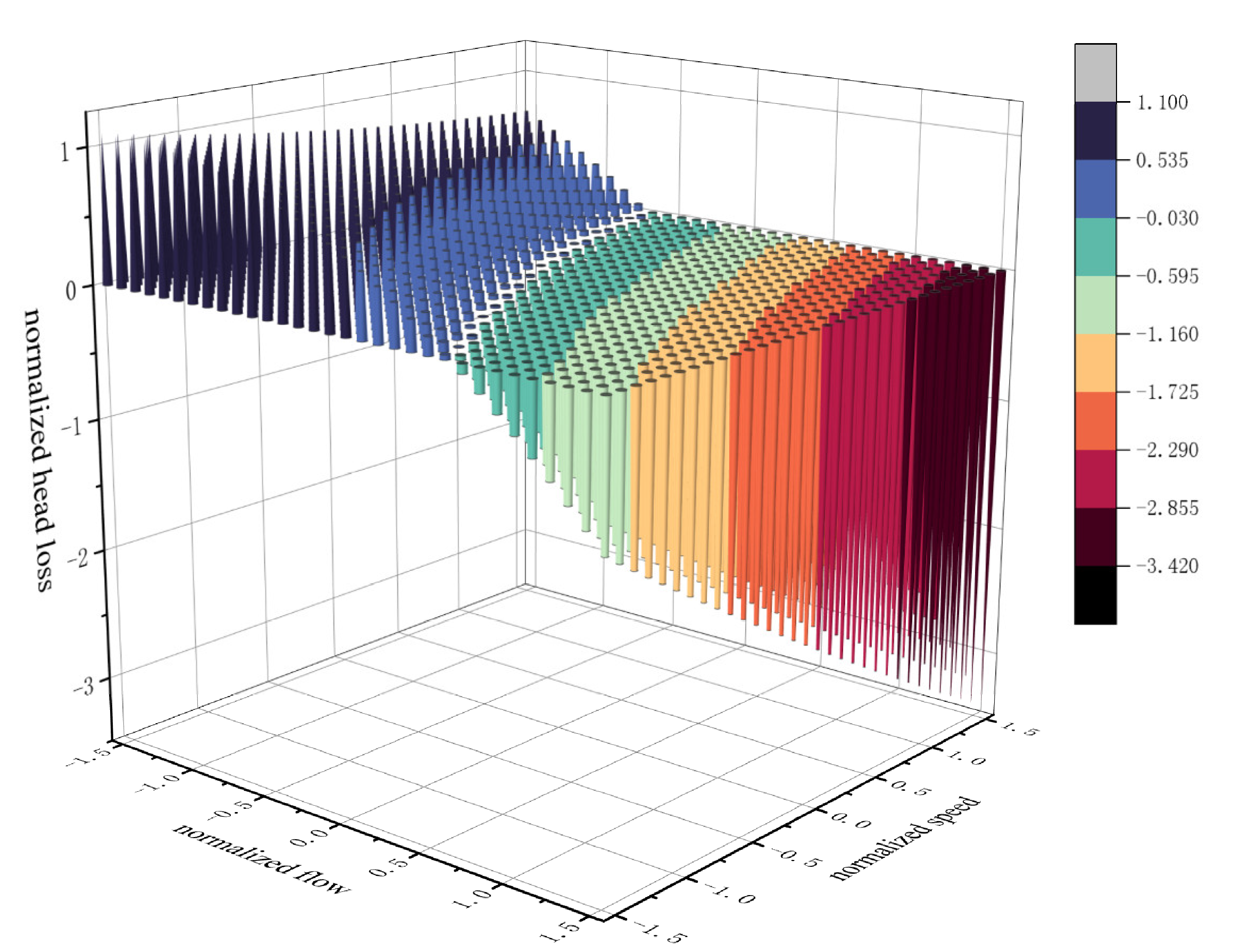
3.3.1. Interaction Term of Filter Flow Rate and Filter Cartridge Speed

(1) The response surface for the interaction factor filter flow rate and filter cartridge speed under the influence of a significant item is established in Figure 5. The response surface analysis reveals that, with a constant filter cartridge speed, the head loss increases as flow rate increases. Similarly, with a constant flow rate, the negative pressure value and head loss relative to speed increase and decrease.

(2) Up to a flow rate of 150 m³/h, the response surface’s upper part exhibits a large high-pressure region with a small curvature and broad area. Optimal curvature results in a significant decrease in the negative pressure value and a sharp increase in head loss. This indicates that an increased irrigation flow rate leads to a more turbulent flow pattern within the filter, thus increasing head loss. However, the contact surface between the filter cartridge and water flow is large, leaving little air above to create compaction effects on the water flow layer. At low rotation speeds, the filter screen clearance exerts a small force on water flow, allowing for easy passage through the filter screen device in the impurity layer. This reduces the collision times between sediment particles and the filter cartridge, resulting in a small head loss.

(3) From the response surface analysis to negative pressure in Figure 5, it is observed that this interaction item exhibits a positive interaction effect on head loss. The energy term has a minor influence on irrigation devices, with the flow term being the primary effect factor for this interaction item. The steepest curvature is small, suggesting that this interaction should be slightly reduced under irrigation-condition satisfaction.

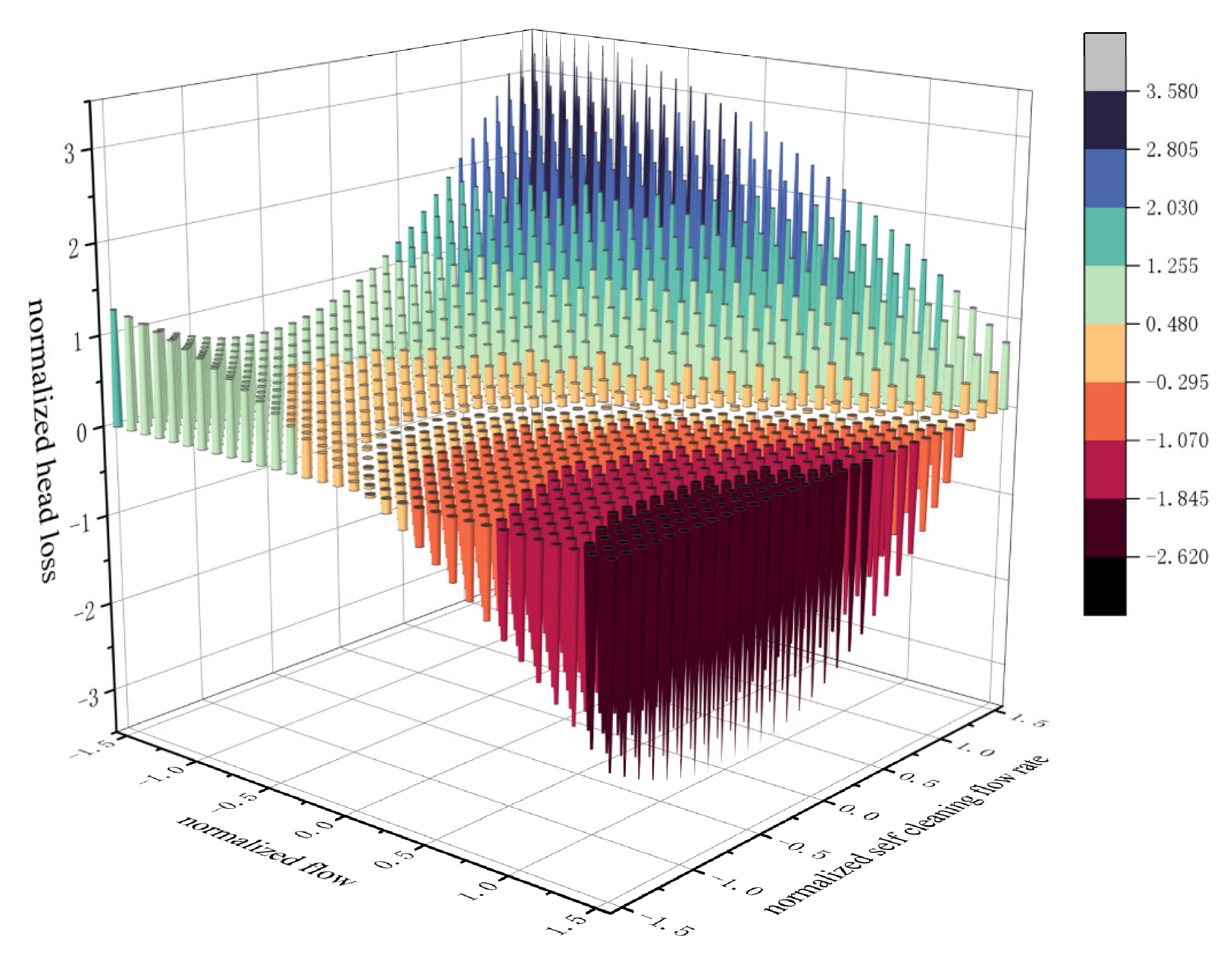
3.3.2. Filter Flow and Self-Cleaning Flow Interaction

(1) This interaction item represents the interaction of filter flow and self-cleaning flow. The response surface, as illustrated in Figure 6, demonstrates that flow rate has a direct impact on negative pressure values. When the self-cleaning device’s flow rate remains constant, increasing flow rate leads to decreased negative pressure values and increased head loss. Conversely, when flow rate is constant, increasing self-cleaning flow rate results in increased negative pressure values and decreased head loss.

(2) As illustrated in Figure 6, when the flow rate is from 130 m³/h to 160 m³/h, the curvature changes more sharply. The upper response surface exhibits a wider range of high negative pressure values, with rapid response value changes and larger curvature. The optimal depth curvature follows, followed by a region of intense change behind the violent change area. The region in front is more inclined towards a mixed state, indicating that irrigation flow and self-cleaning flow are relatively smaller under low flow rates, but more prominent under high flow rates. Consequently, head-loss changes are more pronounced.

(3) Figure 6 reveals that the flow rate positively affects head loss, while self-cleaning flow rate has a suppressing effect. In comparison to the violent change area, both self-cleaning and flow rates are higher, leading to a more mixed area and intense head-loss changes. This should be avoided. The figure demonstrates that this significant term has a negative interaction effect on head loss and plays a significant role in irrigation equipment from an energy perspective. The self-cleaning flow term is the primary influence factor, with the steepest curvature corresponding to a large effect.

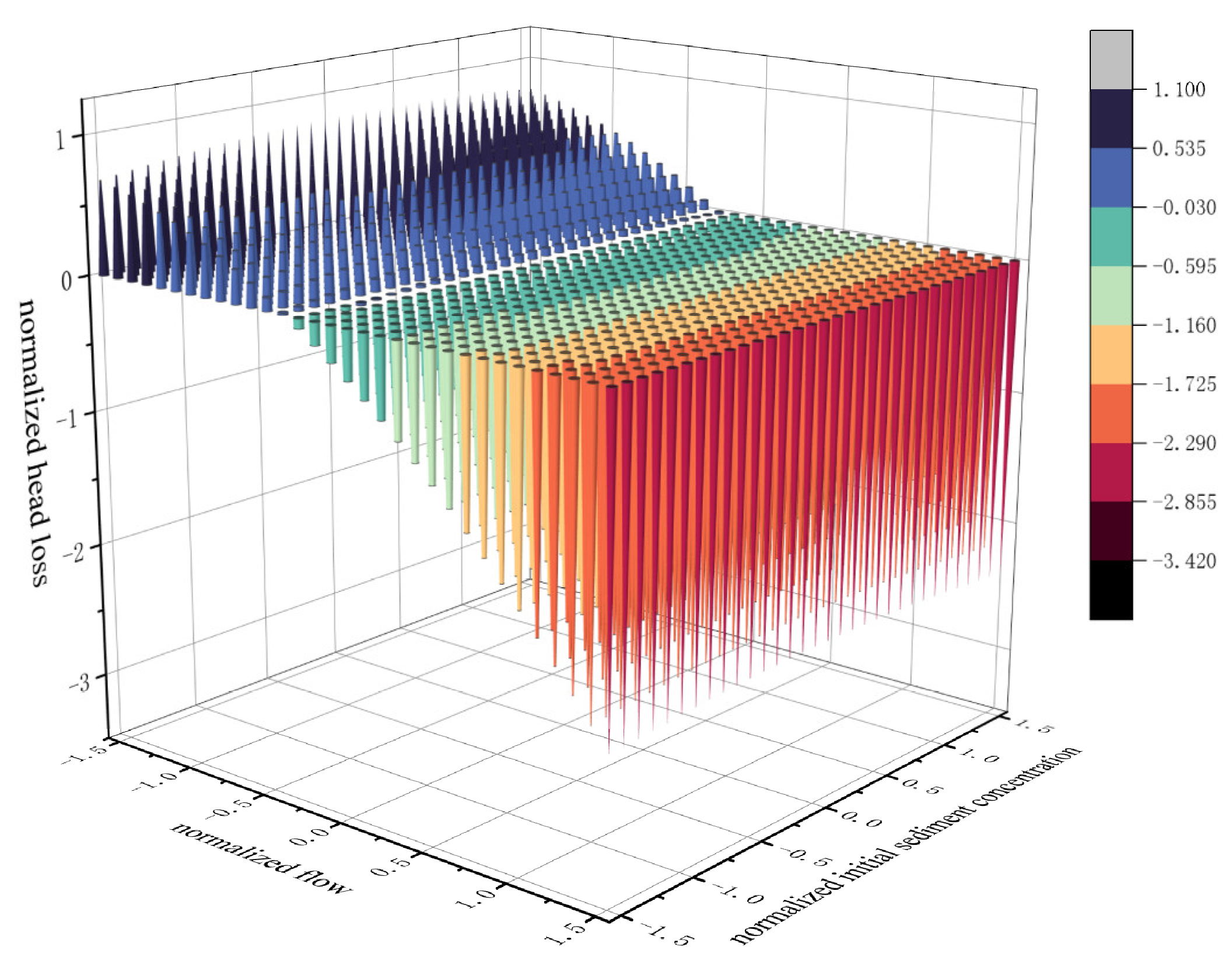
3.3.3. Filter Flow and Initial Sediment Concentration Interaction

(1) This influential term represents the interaction of filter flow and the initial sediment concentration term. The response surface, as depicted in Figure 7, demonstrates that the flow rate has a direct impact on the negative pressure value when the initial sediment concentration remains constant. An increased flow rate leads to decreased negative pressure values and an increased head loss. In contrast, when the flow rate is constant, changes in the head loss relative to initial sediment concentration are minimal.

(2) Figure 7 reveals a small interaction effect of this interaction item on head loss. Compared to the intense change area, the influence of both high initial sediment concentration and discharge is particularly pronounced. This area tends to be more marginal, and head-loss changes are more significant. However, the interaction effect of this interaction item on head loss is not particularly evident.

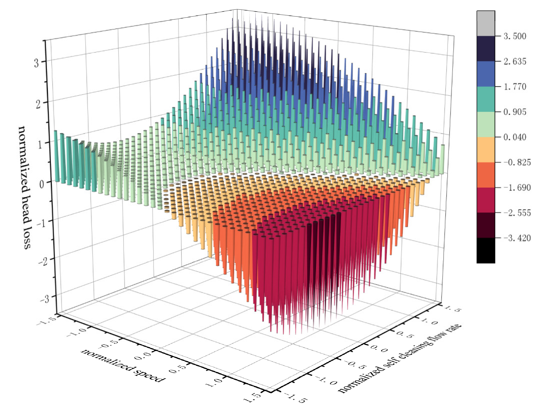
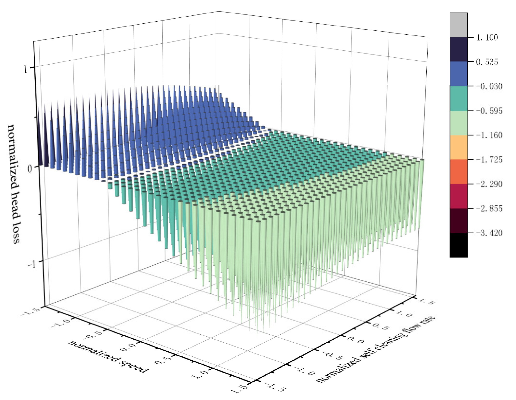
3.3.4. Interaction Term of Cartridge Speed and Self-Cleaning Flow Rate

(1) For the interaction factors of filter cartridge speed and self-cleaning flow rate, its response surface is shown in Figure 8. The response surface analysis of this interaction item to negative pressure value in Figure 7 reveals that when the self-cleaning flow rate remains constant, the negative pressure value decreases with the increase in the cartridge rotation speed term, and the head loss increases accordingly. Conversely, when the cartridge rotation speed term is constant, the negative pressure value increases with the increase in the self-cleaning flow rate, and the head loss decreases.

(2) When the cartridge rotation speed ranges from 2 r/min and the self-cleaning flow rate is approximately 15 m³/h, 20 m³/h, and 28 m³/h, the curvature variation range indicates that the response value changes more sharply compared to Figure 5 and Figure 7. However, the response value variation range is gentler compared to Figure 6. The curvature of the initial optimal path of the response surface graph changes rapidly, with a large area. As the optimal path curvature increases, it signifies a gradual decrease in negative pressure value.

This indicates that the amplitude range of head-loss changes more evenly, the mixing phenomenon is less prominent, and the annular state appears. For the initial sediment concentration and self-cleaning flow rate, the response value change is small, while for the initial sediment concentration and self-cleaning flow rate, the response value change is more intense. This suggests that the head loss decreases with the increase in self-cleaning device flow rate and increases with the increase in cartridge rotation speed. This is because the contact surface between the filter cartridge and water flow is not fully closed, and there is no complete obstruction to the water flow layer. The head loss depends on the collision times and entry probability of sediment particles with the filter cartridge.

(3) This significant term in Figure 7 has a negative interaction effect on head loss, with a large impact on irrigation equipment from an energy perspective. The self-cleaning flow term is the primary influence factor in this interaction item, with the steepest curvature. The interaction term has a negative effect on head loss.

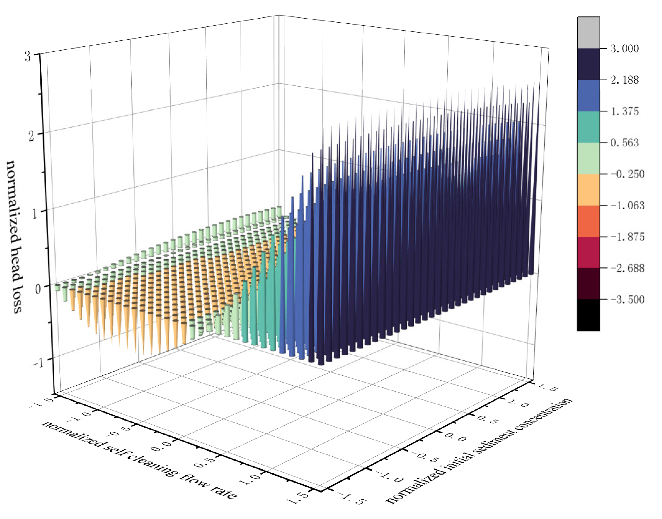
3.3.5. Interaction Term between Filter Cartridge Speed and Initial Sediment Concentration, and Interaction Term between Self-Cleaning Flow Rate and Initial Sediment Concentration

(1) A response surface was established to analyze the interactive effects of filter cartridge speed and initial sand content, as depicted in Figure 9. Additionally, another response surface was developed to examine the interactive effects of self-cleaning flow and initial sand content, as illustrated in Figure 10. According to the response surface analysis, it is observed that when the initial sediment concentration remains constant, the negative pressure value decreases with an increase in filter cartridge rotation speed, leading to an increase in head loss. Similarly, when the initial sediment is constant, the negative pressure value increases as the self-cleaning flow rate increases. However, when either the filter cartridge rotation speed or self-cleaning flow rate is held constant, the change in head loss relative to the initial sediment concentration is not significant. Figure 9 exhibits a gentle change, while Figure 10 reveals a more inclined response value influenced by the self-cleaning flow rate.

(2) Figure 9 and Figure 10 demonstrate that the corresponding interaction term has a minimal impact on head loss. In comparison to the intense change area, the curvature of the response surface tends to be higher in the edge state, indicating a more substantial change in head loss.

3.4. Interaction Correction

To account for interaction effects, a response surface analysis was employed to modify the regression equation compared to previous head loss analyses. The results are presented in

Table 6. Modify the model.

Head Loss	A	B	C	AB	BC	A2	C2
−20.28	−1.83667	−0.82167	1.526667	−0.3775	0.2325	−0.43542	1.247083
significance level	<0.0001	<0.0001	< 0.0001	0.0033	0.0467	0.0001	<0.0001
R2	0.9930

.

Table 6 presents the optimized model derived from the response surfaces depicted in Figure 5, Figure 6, Figure 7, Figure 8, Figure 9 and Figure 10. The results highlight a substantial improvement in the determination coefficient, indicating a stronger correlation between the variables.

By integrating the response surfaces in Figure 5, Figure 6, Figure 7, Figure 8, Figure 9 and Figure 10 and employing the optimized model, a total of 100 solutions were obtained by utilizing the method of determining the optimal slope of the response surface. The optimization plan is presented in Figure 11 as a data diagram. From this diagram, the best solution was identified by removing the standardization. It was found that, at a flow rate of 121.687 m³·h⁻¹, a rotation speed of 1.331 r·min⁻¹, a self-cleaning flow rate of 19.980 m³·h⁻¹, and an initial sand content of 0.261 g·L⁻¹, the minimum head loss obtained was 21.671 kPa. This result signifies the optimal combination of parameters that leads to the lowest head loss. The optimization plan outlined in Figure 11 serves as a reference for future research in this area. Researchers and practitioners can utilize this plan to guide their decision-making process when designing and operating filtration systems, with the aim of minimizing head loss and maximizing system performance. It should be noted that the methodology employed in this study, which involved combining response surfaces and an optimized model, demonstrates the effectiveness of such an approach in understanding complex relationships between multiple factors. By visualizing the data in Figure 5, Figure 6, Figure 7, Figure 8, Figure 9 and Figure 10 and applying the method of finding the optimal slope of the response surface, a comprehensive set of solutions was obtained, leading to the identification of the best possible combination of parameters.

The different combinations of lines in Figure 11 represent different optimal solutions obtained by adjusting parameters through model algorithms when applying the response surface method. These lines demonstrate the relationship between parameters and system performance, and help researchers determine the possible optimal combination of parameters.

4. Discussion

Although numerous studies have explored the factors influencing filter performance, few have comprehensively considered the interactions among multiple factors [27,28,29,30,31]. By introducing interaction terms, this study not only unveils the complex relationships among these factors but also enhances the predictive accuracy of the model. This aligns with the recent emphasis in academic journals on model complexity and predictive capability [32].

Furthermore, the findings of this study corroborate some of the latest literature, further validating the model’s reliability. Several studies have pointed out the significant impact of irrigation flow rate on filter performance, which concurs with the predominant role of irrigation flow rate observed in this study. Additionally [31,32,33], this study identifies the important influence of self-cleaning flow rate and filter cartridge speed on head loss, echoing discussions in the literature about filter self-cleaning functions and cartridge design optimization [32].

However, compared to the existing literature, this study reveals some novel findings [34,35]. For example, the interaction between irrigation flow rate and filter cartridge speed has a particularly significant effect on head loss, highlighting the need to pay closer attention to the combination of these two factors during irrigation system design. Moreover, the strongest contribution from the self-cleaning flow rate underscores the importance of self-cleaning functionality in filter design.

Lastly, this study acknowledges certain limitations compared to the existing literature. Specifically, it focuses on four primary test factors, while acknowledging that actual irrigation systems may involve other potential influencing factors. Future research could expand the model’s applicability by considering additional factors and their interactions on filter performance. Moreover, validating the model’s universal applicability and reliability across various types of filters would be a worthwhile pursuit [36].

5. Conclusions

• Integrating four key test factors, including irrigation flow, filter cartridge speed, self-cleaning flow, and initial sand content, we developed a head loss model for pressureless mesh filters used in farmland irrigation. After refining the response surface, the model showed a significant improvement with a coefficient of determination of 98.61%.
• The total irrigation flow had a 17.20% higher contribution than the self-cleaning flow rate, while the initial sand content had the smallest contribution at 0.0166. Additionally, the self-cleaning flow rate had a 46.18% higher contribution than the filter cartridge speed, and the filter cartridge speed had a 96.34% higher contribution than the initial sand content.
• The interaction term between irrigation flow and filter cartridge speed had a contribution 218.25% higher than the interaction term between irrigation flow and initial sand content. The self-cleaning flow rate’s self-interaction had the highest contribution, while the filter cartridge speed’s self-interaction had the smallest contribution.
• By optimizing the response surface and the model, the optimal parameters were determined to be an irrigation flow rate of 121.687 m³·h⁻¹, a filter cartridge speed of 1.331 r·min⁻¹, a self-cleaning flow rate of 19.980 m³·h⁻¹, and an initial sand content of 0.261 g·L⁻¹, resulting in a minimum head loss of 21.671 kPa.

References

1. Niu, W.; Wu, P.; Li, J.; Shao, H. One of frontiers in agricultural and environmental biotechnology for the arid regions: Micro-pressure drip irrigation technology theory and practices. Afr. J. Biotechnol. 2010, 9, 2891–2897. [Google Scholar]
2. Yildiz, H.; Kadayifci, A. Design and Operation Analysis of Drip Irrigation Systems Used in the Irrigation of Cherry Orchards in Isparta-Uluborlu Region, Turkey. Appl. Ecol. Environ. Res. 2018, 16, 3131–3143. [Google Scholar] [CrossRef]
3. Tian, C.; Lv, Z.; Song, Y.; Zhang, H. Increasing the cotton yield and improving the ecology in cotton fields by utilizing the properties of natural resources in Xinjiang, China. In Ecosystems Dynamics, Ecosystem-Society Interactions, and Remote Sensing Applications for Semi-Arid and Arid Land; SPIE: Bellingham, WA, USA, 2003; Volume 4890, pp. 809–819. [Google Scholar] [CrossRef]
4. Yu, L.M.; Li, J.L.; Li, N.; Wang, J.Y.; Wang, D.R. Wear Behavior and Vortex Characteristics of Y-Type Screen Filters with Various Inclination Angles and Inlet Flow Velocities: Numerical and Experimental Study. J. Irrig. Drain. Eng. 2023, 149, 04023014. [Google Scholar] [CrossRef]
5. Sanderson, S.L.; Roberts, E.; Lineburg, J.; Brooks, H. Fish mouths as engineering structures for vortical cross-step filtration. Nat. Commun. 2016, 7, 11092. [Google Scholar] [CrossRef] [PubMed]
6. Bayer-Raich, M.; Jordana, S.; Jaime, O.M.; Lynch, T.D.; McGillicuddy, K.B.; Guimera, J.; Jaime, M.J. Numerical Modeling of Head Losses in Different Types of Well Screens. Ground Water 2022, 60, 747–756. [Google Scholar] [CrossRef] [PubMed]
7. Houben, G.J.; Wachenhausen, J.; Morel, C.R.G. Effects of ageing on the hydraulics of water wells and the influence of non-Darcy flow. Hydrogeol. J. 2018, 26, 1285–1294. [Google Scholar] [CrossRef]
8. Tao, H.; Shen, P.; Li, Q.; Jiang, Y.; Yang, W.; Wei, J. Research on head loss of pre-pump micro-pressure filter under clean water conditions. Water Supply 2022, 22, 3271–3282. [Google Scholar] [CrossRef]
9. Demir, V.; Yürdem, H.; Yazgi, A.; Degirmencioglu, A. Determination of the head losses in metal body disc filters used in drip irrigation systems. Turk. J. Agric. For. 2009, 33, 219–229. [Google Scholar] [CrossRef]
10. Cano, N.D.; Camargo, A.P.; Ait-Mouheb, N.; Muniz, G.L.; Guarnizo, J.A.Y.; Pereira, D.J.S.; Frizzone, J.A. Optimisation of the filter housing dimensions of an automatic flushing strainer-type filter. Biosyst. Eng. 2022, 219, 25–37. [Google Scholar] [CrossRef]
11. Arbat, G.; Pujol, T.; Puig-Bargués, J.; Duran-Ros, M.; Barragán, J.; Montoro, L.; de Cartagena, F.R. Using Computational Fluid Dynamics to Predict Head Losses in the Auxiliary Elements of a Microirrigation Sand Filter. Trans. Asabe 2011, 54, 1367–1376. [Google Scholar] [CrossRef]
12. Liu, F.; Liu, Y.A. Uplink scheduling for LTE-advanced system. In Proceedings of the 2010 IEEE International Conference on Communication Systems, Singapore, 17–19 November 2010; pp. 316–320. [Google Scholar]
13. Samuel, M.P.; Senthilvel, S.; Tamilmani, D.; Mathew, A.C. Performance evaluation and modelling studies of gravel–coir fibre–sand multimedia stormwater filter. Environ. Technol. 2012, 33, 2057–2069. [Google Scholar] [CrossRef] [PubMed]
14. Boyer, D.G. Assessment of a sinkhole filter for removing agricultural contaminants. J. Soil Water Conserv. 2008, 63, 47–52. [Google Scholar] [CrossRef]
15. Carrión-Coronel, E.; Ortiz, P.; Nanía, L. Physical Experimentation and 2D-CFD Parametric Study of Flow through Transverse Bottom Racks. Water 2022, 14, 955. [Google Scholar] [CrossRef]
16. Blocken, B.; Gualtieri, C. Ten iterative steps for model development and evaluation applied to Computational Fluid Dynamics for Environmental Fluid Mechanics. Environ. Model. Softw. 2012, 33, 1–22. [Google Scholar] [CrossRef]
17. Shehzad, M.A.; Bashir, A.; Ul Amin, M.N.; Khosa, S.K.; Aslam, M.; Ahmad, Z. Reservoir Inflow Prediction by Employing Response Surface-Based Models Conjunction with Wavelet and Bootstrap Techniques. Math. Probl. Eng. 2021, 2021, 4086918. [Google Scholar] [CrossRef]
18. Hassan, M.M.; Yun, J.S.; Rahman, M.M.; Choo, Y.W.; Han, J.T.; Kim, D. Centrifugal Test Replicated Numerical Model Updating for 3D Strutted Deep Excavation with the Response-Surface Method. Appl. Sci. 2022, 12, 665. [Google Scholar] [CrossRef]
19. Kluz, R.; Habrat, W.; Bucior, M.; Krupa, K.; Sep, J. Multi-criteria optimization of the turning parameters of Ti-6Al-4V titanium alloy using the Response Surface Methodology. Eksploat. Niezawodn.-Maint. Reliab. 2022, 24, 668–676. [Google Scholar] [CrossRef]
20. Zalewski, M.J.; Maminski, M.L.; Parzuchowski, P.G. Synthesis of Polyhydroxyurethanes-Experimental Verification of the Box-Behnken Optimization Model. Polymers 2022, 14, 4510. [Google Scholar] [CrossRef] [PubMed]
21. Sharma, M.; Janardhan, G.; Sharma, V.K.; Kumar, V.; Joshi, R.S. Comparative prediction of surface roughness for MAFM finished aluminium/silicon carbide/aluminium trioxide/rare earth oxides (Al/SiC/Al2O3)/REOs) composites using a Levenberg–Marquardt Algorithm and a Box–Behnken Design. Proc. Inst. Mech. Eng. Part E J. Process Mech. Eng. 2021, 236, 790–804. [Google Scholar] [CrossRef]
22. Toprak, D.; Demir, Ö.; Uçar, D. Extracellular azo dye oxidation: Reduction of azo dye in batch reactors with biogenic sulfide. Phosphorus Sulfur Silicon Relat. Elem. 2022, 197, 927–933. [Google Scholar] [CrossRef]
23. Eltas, O.; Topal, M. Using Multivariate Analysis of Covariance in Genetic Parameter Estimation. Fresenius Environ. Bull. 2022, 31, 2015–2024. [Google Scholar]
24. Jamshidi, L.; Declercq, L.; Fernandez-Castilla, B.; Ferron, J.M.; Moeyaert, M.; Beretvas, S.N.; Van den Noortgate, W. Multilevel meta-analysis of multiple regression coefficients from single-case experimental studies. Behav. Res. Methods 2020, 52, 2008–2019. [Google Scholar] [CrossRef] [PubMed]
25. Wang, R.; Xu, X.Z. Least Favorable Direction Test for Multivariate Analysis of Variance in High Dimension. Stat. Sin. 2021, 31, 723–747. [Google Scholar] [CrossRef]
26. Kostousova, E.K. External Polyhedral Estimates of Reachable Sets of Discrete-Time Systems with Integral Bounds on Additive Terms. Math. Control. Relat. Fields 2021, 11, 625–641. [Google Scholar] [CrossRef]
27. Zong, Q.L.; Zheng, T.G. Numerical Simulation on Flow Field of Screen Filter for Drip Irrigation in Field. In Proceedings of the International Conference on Civil, Architectural and Hydraulic Engineering (ICCAHE 2012), Zhangjiajie, China, 10–12 August 2012. [Google Scholar]
28. Chi, Y.; Yang, P.; Ma, Z.; Wang, H.; Liu, Y.; Jiang, B.; Hu, Z. The Study on Internal Flow Characteristics of Disc Filter under Different Working Condition. Appl. Sci. 2021, 11, 7715. [Google Scholar] [CrossRef]
29. Milstein, A.; Feldlite, M. Relationships between clogging in irrigation systems and plankton community structure and distribution in wastewater reservoirs. Agric. Water Manag. 2014, 140, 79–86. [Google Scholar] [CrossRef]
30. Zhang, W.; Cai, J.; Zhai, G.; Song, L.; Lv, M. Experimental Study on the Filtration Characteristics and Sediment Distribution Influencing Factors of Sand Media Filters. Water 2023, 15, 4303. [Google Scholar] [CrossRef]
31. Yamamoto, T.; Fujiyama, H.; Miyamoto, K.; Hatanaka, J.; Wen, G.; Asae, A. Optimizing water cleaning system for microirrigation in the Tokaku Irrigation Project of Japan. In Proceedings of the 4th National Irrigation Symposium, Phoenix, AZ, USA, 14–16 November 2000. [Google Scholar]
32. Coelho, R.D.; De Almeida, A.N.; Costa, J.D.O.; De Sousa Pereira, D.J. Mobile drip irrigation (MDI): Clogging of high flow emitters caused by dragging of driplines on the ground and by solid particles in the irrigation water. Agric. Water Manag. 2022, 263, 107454. [Google Scholar] [CrossRef]
33. Graciano-Uribe, J.; Pujol, T.; Puig-Bargues, J.; Duran-Ros, M.; Arbat, G.; Ramirez de Cartagena, F. Assessment of Different Pressure Drop-Flow Rate Equations in a Pressurized Porous Media Filter for Irrigation Systems. Water 2021, 13, 2179. [Google Scholar] [CrossRef]
34. Jiao, Y.; Feng, J.; Liu, Y.; Yang, L.; Han, M. Sustainable operation mode of a sand filter in a drip irrigation system using Yellow River water in an arid area. Water Supply 2020, 20, 3636–3645. [Google Scholar] [CrossRef]
35. De Deus, F.P.; Mesquita, M.; Testezlaf, R.; De Almeida, R.C.; de Oliveira, H.F.E. Methodology for hydraulic characterisation of the sand filter backwashing processes used in micro irrigation. MethodsX 2020, 7, 100962. [Google Scholar] [CrossRef] [PubMed]
36. Song, L.; Cai, J.; Zhai, G.; Feng, J.; Fan, Y.; Han, J.; Hao, P.; Ma, N.; Miao, F. Comparative Study and Evaluation of Sediment Deposition and Migration Characteristics of New Sustainable Filter Media in Micro-Irrigation Sand Filters. Sustainability 2024, 16, 3256. [Google Scholar] [CrossRef]
Figure 1. Schematic diagram of the overall structure of the pressure free mesh filter: (1) float, (2) rotating motor, (3) dirt baffle, (4) filter cylinder, (5) main bracket, and (6) self-cleaning device. The unit of size in the figure is 1 mm.
Agriculture 14 00788 g001
Figure 2. Experimental device diagram: (1) water return device, (2) electromagnetic flowmeter, (3) electromagnetic pump, (4) stirring device, (5) filtration system, and (6) high-precision negative pressure gauge. The unit of size in the figure is 1 mm.
Agriculture 14 00788 g002
Figure 3. Sediment particle grad diagram.
Agriculture 14 00788 g003
Figure 4. Analysis of the contribution parameters and confidence intervals of filter factors.
Agriculture 14 00788 g004
Figure 5. Normalization of filter flow and cartridge speed interaction item to negative pressure value.
Agriculture 14 00788 g005
Figure 6. Normalization of filter flow and self-cleaning flow interaction to negative pressure values.
Agriculture 14 00788 g006
Figure 7. Normalization of filter flow and initial sediment interaction to negative pressure values.
Agriculture 14 00788 g007
Figure 8. Normalization of cartridge speed and self-cleaning flow interaction term to the negative pressure value.
Agriculture 14 00788 g008
Figure 9. Normalization of cartridge speed and initial sediment interaction to negative pressure value.
Agriculture 14 00788 g009
Figure 10. Normalization of self-cleaning flow and initial sediment interaction to negative pressure value.
Agriculture 14 00788 g010
Figure 11. Cartridge speed and initial sediment interaction to negative pressure value.
Agriculture 14 00788 g011