Worldwide Examination of Magnetic Responses to Heavy Metal Pollution in Agricultural Soils

Abstract

Over the last decade, a large number of studies have been conducted on heavy metals and magnetic susceptibility (${\mathsf{\chi }}_{\mathrm{l}\mathrm{f}}$) measurement in soils. Yet, a global understanding of soil contamination and magnetic responses remains elusive due to the limited scope or sampling sites of these studies. Hence, we attempted to explore a pollution proxy on a global scale. Through a meta-analysis of data from 102 published studies, our research aimed to provide a worldwide overview of heavy metal pollution and magnetic responses in agriculture soils. We mapped the geographic distribution of nine heavy metals (Cr, Cu, Zn, Pb, Ni, As, Cd, Mn, and Fe) in agricultural soils and explored their pollution sources and contributions. Since 2011, The accumulation of heavy metals has escalated, with industrial activities (31.5%) being the largest contributor, followed by agricultural inputs (27.1%), atmospheric deposition (22.66%), and natural sources (18.74%). The study reports ${\mathsf{\chi }}_{\mathrm{l}\mathrm{f}}$ ranging from 6.45 × 10⁻⁸ m³/kg to 319.23 × 10⁻⁸ m³/kg and ${\mathsf{\chi }}_{\mathrm{f}\mathrm{d}}$ from 0.59% and 12.85%, with the majority of the samples being below 6%, indicating heavy metal influence mainly from human activities. Pearson’s correlation and redundancy analysis show significant positive correlations of Pb, Zn, and Cu with ${\mathsf{\chi }}_{\mathrm{l}\mathrm{f}}$ (r = 0.51–0.53) and Mn and Fe with ${\mathsf{\chi }}_{\mathrm{f}\mathrm{d}}$ (r = 0.50–0.53), while Pb, Zn, Cu, and As metals were shown to be key factors of variation in magnetic response. The average heavy metal pollution load index of 2.03 suggests moderate global agricultural soil pollution, with higher heavy metal contamination in areas of high ${\mathsf{\chi }}_{\mathrm{l}\mathrm{f}}$. Regression analysis confirms soil is considered to be non-polluted below ${\mathsf{\chi }}_{\mathrm{l}\mathrm{f}}$ of $26\times {10}^{-8} {\mathrm{m}}^3/\mathrm{k}\mathrm{g}$ and polluted above this threshold, with all contamination factors of metals showing a linear correlation with ${\mathsf{\chi }}_{\mathrm{l}\mathrm{f}}$ (R = 0.72), indicating that a significant relationship between ${\mathsf{\chi }}_{\mathrm{l}\mathrm{f}}$ and the geochemical properties of soils continues to exist on a global scale. This study provides new insights for large-scale agricultural soil quality assessment and magnetic response.

1. Introduction

Soil contamination by heavy metals (HMs) is a globally acknowledged environmental concern [1]. Over the last three centuries, industrialization, synthetic chemical production, rapid urbanization, and intensified agriculture have heightened the exposure of soil to HMs from human activities, leading to their accumulation [2,3]. Currently, numerous countries, including the United States, Europe, Australia, China, and India (refs. [4,5,6,7,8,9]), report varying degrees of soil HM pollution. Priority pollutants typically include cadmium, chromium, arsenic, lead, copper, zinc, nickel, and other HMs, known for their toxicity, bioconcentration, and persistence [10,11]. For example, agricultural soils in northern Italy and topsoil in Mexican cities have exhibited excessive levels of Pb, Zn, Cu, and As, surpassing pollution thresholds and threatening human health [12,13]. Influenced by agricultural soil physicochemical properties, external inputs, and biological factors, there are numerous sources of HM enrichment, and the spatial pattern of HMs in soil shows a high degree of heterogeneity [14]. Therefore, identifying the sources of these challenges and analyzing their collective accumulation patterns is challenging. Globally, the primary sources of soil HMs primarily stem from natural sources (e.g., soil parent materials) and various anthropogenic sources, including metal ore mining and smelting, agricultural and horticultural practices, sewage sludge treatment, fossil fuel combustion, the metallurgical industry, electronics, chemical, and other manufacturing sectors, waste disposal, recreational shooting and fishing, and military operations and training [15]. The elucidation of the origins of geochemical elements, such as Cr, Cu, Zn, Pb, Ni, As, and Cd, which are pivotal indicators in particular parent materials, soil action, and processes, relies on their geochemical behavior within the soil environment [16]. This behavior encompasses aspects such as mobility, organic complexation, and adsorption by inorganic colloids, along with the source characteristics including mineral properties, elemental composition, and susceptibility to weathering, as well as the general environmental context of the study area [17,18]. The interpretation of these geochemical studies, however, is markedly challenging in pinpointing sources due to the interplay between anthropogenic and natural factors [19]. A detailed understanding of the geographic distribution of HM concentrations across different regions, the identification of source contributions, and the extensive heterogeneity in soil magnetism are critical for the assessment of the risk of HM contamination, but much remains to be done in this area.

In the investigation of soil contamination by HMs, researchers often employ a combination of geochemical elemental analysis and environmental magnetic techniques to determine the extent of contamination in soils and sediments [20,21,22,23,24,25,26,27,28]. The environmental magnetic method is simply the study of magnetic mineralogy in natural and man-made samples by measuring the induced magnetization and remanent magnetic response of natural and man-made samples when they are exposed to a magnetic field. This approach not only applies the measured magnetic parameters to pollution screening and monitoring but also effectively quantifies and characterizes particulate matter from industrial, traffic, and municipal sources and precisely identifies the source of pollutants while tracking their development history [29,30,31,32]. It significantly contributes to understanding various soil-related issues, such as sedimentary and diagenetic processes [33,34,35,36]. Previous research has led to the creation of national-scale topsoil magnetic databases in countries including Australia, Bosnia and Herzegovina, Bulgaria, and France, employing advanced geostatistics to explore the potential of magnetic features as indicators of specific soil chemical and physical properties [37,38,39,40,41]. Furthermore, recent studies have increasingly focused on the semi-quantitative assessment of contamination levels for pollutants like Cu, Pb, Zn, Cr, V, and Mn using magnetic parameters. For example, Hanesch et al. assessed magnetic susceptibility in extensive soil areas of eastern Austria to track HM contamination [42]. Nele Delbecque et al. examined 103 soil horizons in Ghent, Belgium, uncovering differences in anthropogenic and diagenetic contributions in soils and demonstrating that volume-specific magnetic susceptibility effectively predicts HM enrichment [19]. Similarly, research in Mexico and Poland has linked magnetic properties to HM concentrations (Fe, Pb, Cu, Zn, Ni, Cr, and V), providing empirical evidence that anthropogenic Fe/ferromagnetic minerals contribute to increased magnetic susceptibility values in topsoil, indicative of a symbiotic relationship [13,43]. Chaparro et al. investigated magnetic screening and heavy metal pollution in soils from the Marambio Station in Antarctica, offering insights into the magnetic responses to heavy metal pollution in a unique environment. Their research revealed a significant reduction in pollution as a result of national remediation efforts. These studies contribute valuable insights to our understanding of soil contamination and magnetism [26,44]. In addition to traditional analytical methods, recent advancements have introduced the use of fuzzy models in magnetic monitoring. For instance, a study by Chaparro proposed a magnetic index (IMC) that leverages fuzzy clustering, fuzzy arithmetic, and a fuzzy inference system to analyze relationships between the IMC and PLI, suggesting a promising approach for broader application in environmental matrices such as soils and sediments [45]. The application of magnetic susceptibility measurement techniques for the characterization of soils and geochemistry has consistently been a focal point of research. Despite this, the majority of research linking soil HM contamination to magnetic susceptibility has been limited to small-scale studies or those with restricted sampling sites, primarily due to constraints in large-scale soil sampling and analysis capabilities. As a result, a comprehensive understanding of this relationship on a global level remains elusive.

The magnetic parameters mentioned in this study include ${\mathsf{\chi }}_{\mathrm{l}\mathrm{f}}$ (low-frequency magnetic susceptibility) and ${\mathsf{\chi }}_{\mathrm{f}\mathrm{d}}$ (frequency-dependent susceptibility). We employed correlation analysis (CA) to investigate the relationship between magnetic parameters and HMs, discussed the commonality of HM pollution sources, and combined redundancy analysis (RDA) to elucidate the impact of different magnetic response sampling points on the accumulation of HMs in soil. This analysis enabled us to identify the key factors responsible for variations in magnetic response. In addressing soil pollution sources, source apportionment analysis frequently estimates the quantity, proportion, and nature of these sources. Researchers have employed various techniques, including PCA, APCS/MLR, UNMIX, and PMF, for source identification in HM contamination [33,34,46,47,48,49,50,51]. Prior research has employed partition-computing-based Positive Matrix Factorization (PC-PMF) to showcase its efficacy in conducting source assignment calculations on a large scale [52]. The findings underscore the considerable benefits of partitioning calculations in scenarios with spatial heterogeneity from multiple sources. This is of great value in expanding the application of receptor modeling, especially in large-scale fields. For this study, we reviewed 102 scientific papers from a database. The vast database of agricultural soils presents significant opportunities for broadening receptor modeling applications, offering fresh perspectives on the magnetic and geochemical characterization of soils.

In this study, we summarized the published statistical results with the aim of (1) exploring the geographic distribution characteristics of agricultural soil HMs, analyzing the reasons for the geographic differences, and quantifying their regional source contributions using PC-PMF; (2) characterizing the magnetic properties of soils in the globally delineated regions to understand the magnetic heterogeneity of the agricultural soil system; (3) revealing the relationship between different HM concentrations and magnetic susceptibility by Pearson’s and redundancy analysis (RDA), as well as the factors affecting the magnetic response differences; and (4) calculating the contamination factor (CF) and pollution load index (PLI) for each element, establishing the regression equations between the CF and the logarithmic magnetic susceptibility (${\mathrm{l}\mathrm{n}\mathsf{\chi }}_{\mathrm{l}\mathrm{f}}$), and analyzing the differences between the areas sampled by the high-value and low-value ${\mathsf{\chi }}_{\mathrm{l}\mathrm{f}}$, to determine the magnetic parameter as the contamination of HM proxies and reveal differences in anthropogenic, diagenetic, and soil contributions to soil neutralization.

2. Materials and Methods

2.1. Data Extraction

A thorough literature review was performed using the Web of Science and Elsevier databases, employing search terms such as ‘agricultural soil’ or ‘farmland soil’, ‘heavy metal’, and individual elements (Cr, Cu, Zn, Pb, Ni, As, Cd, Mn, or Fe) in conjunction with ‘magnetic susceptibility’. For inclusion in this meta-analysis, studies were required to satisfy specific criteria: (1) conducted within the timeframe of 2004 to 2023: this period is chosen to reflect recent heavy metal pollution trends and to ensure comparability of data from standardized environmental monitoring practices; (2) field studies examining topsoil at depths of 0–20 cm: focusing on surface soil captures the initial zone of heavy metal accumulation and dynamics due to human and environmental factors; (3) provision of detailed information on the study area’s size, latitude and longitude and the number of soil sampling sites: these details enable researchers to assess the representativeness of the study area, enhance the reproducibility of the data and contextual analysis, and facilitate comparisons in similar geographic settings; and (4) a sample size exceeding 30: a larger sample size ensures statistical reliability and the generalizability of the findings, reflecting robust data collection in the area of study (Figure 1). The geographical locations of the studies included in the meta-analysis are shown in Figure 1.

In order to explore the regional differences in the distribution of HMs in more detail, the world was divided into 12 regions based on the United Nations Statistics Division [53]. These regions are based on similar socio-economic parameters of countries belonging to the same region. This meta-analysis synthesized a total of 429 independent observations from 102 studies (

Table 1. Number of country groups and reports used for meta-analysis. The exact link for Our World in Data’s region definitions is: https://ourworldindata.org/world-region-map-definitions.

Region	Abbreviation for Region or Country	Number of Records
Australia and New Zealand	ANZ	18
Europe	EU	71
Africa	AF	26
Northern America—USA	USA	36
Rest of America	ROA1	21
Central America—Caribbean	CA	14
Middle East	ME	15
Southern America—Brazil	BR	25
Southern Asia—India	IN	37
Northern China	NC	79
Southern China	SC	70
Rest of Asia	ROA2	17
World	-	429

).

2.2. PC-PMF Model

Positive Matrix Factorization (PMF), developed by Paatero and Tapper in the early 1990s [54], is a factorization method that quantifies the contribution of source composition to a given sample F. Central to the PMF model is establishing a chemical mass balance between the concentrations of various species and their source profiles, as detailed in Equation (1). In this equation, P denotes the number of factors, F signifies the species within each source profile, and G represents the mass contribution of each factor to individual samples. Our analysis employed specific equations, in line with Environmental Protection Agency (EPA) PMF5.0 guidelines, to assign HMs to their respective sources.

$${\mathrm{X}}_{\mathrm{i}\mathrm{j}}={\sum }_{\mathrm{k}=1}^{\mathrm{p}}{\mathrm{G}}_{\mathrm{i}\mathrm{k}}{\mathrm{F}}_{\mathrm{i}\mathrm{k}}+{\mathrm{E}}_{\mathrm{i}\mathrm{j}}$$

(1)

where X_ij is the matrix of sample concentrations; G_ik is the contribution of each factor to any given sample; F_ij is the matrix of P-source chemical compositions; and E_ij is the matrix of residues for each sample. The contributions of the factors and the objective function ‘Q’, which is essential for minimizing the PMF model, are derived from these profiles and defined as follows:

$$\mathrm{Q}=\sum _{\mathrm{i}=1}^{\mathrm{n}}\sum _{\mathrm{j}=1}^{\mathrm{m}}{\left(\frac{{\mathrm{E}}_{\mathrm{i}\mathrm{j}}}{{\mathrm{U}}_{\mathrm{i}\mathrm{j}}}\right)}^2$$

(2)

where Q is the sum of the squares of the differences between the original dataset (X_ij) and the PMF output (G_ij F_ij) weighted by the measurement uncertainty (U_ij). For a comprehensive understanding of the PMF receptor model, further details can be found in Paatero et al. and Brown et al. [55].

PC-PMF is a computational method developed from the PMF model, introduced by Jin Wu et al., and it possesses substantial advantages when dealing with large-scale or geographically dispersed datasets. Previous research has utilized Partitioned Computation of Positive Matrix Factorization (PC-PMF) to demonstrate its effectiveness in extensive source allocation calculations [52]. In this model, data are divided into several partitions or subsets, each representing a different geographical area or type of data. The PMF model is then applied independently to each subset, which helps in better understanding the regional characteristics or contributions of local sources. The world was segmented into 12 countries and regions following the United Nations Statistics Division (Table 1). This segmentation facilitated the examination of HM sources in each of the 12 sub-regions and the entire region collectively. The contribution of primary sources in each zone to the overall study area was ascertained by computing each zone’s contribution and then applying a weighting based on the ratio of the number of reports in each zone to the total global document count. The weighting calculation formula is

$${\mathrm{G}}_{\mathrm{k}}={\sum }_{\mathrm{i}=1}^{\mathrm{n}}{\mathrm{G}}_{\mathrm{m}\mathrm{k}}\frac{{\mathrm{A}}_{\mathrm{m}}}{\mathrm{A}}$$

(3)

where G_k is the contribution of the kth source factor to the whole region, G_mk is the contribution of the kth source factor to the mk region, A_m is the number of reports in the m_k region, and A is the number of reports in the whole study region. This calculation method was proposed by Jin Wu [52], whose study weighted and summed the area of each region as a proportion of the entire study area, and our calculation method is slightly different in that weighting, and summing the number of documents in each region as a proportion of the total number of documents globally is a more accurate method due to the uneven distribution of sampling points in our study.

2.3. Multivariate Statistical Analysis

The Pearson correlation coefficient is a statistical method used to measure the strength and direction of the linear relationship between two quantitative variables. Typically represented by r, its value ranges from −1 to +1, with values closer to 1 or −1 indicating a stronger relationship [56]. Based on this principle, we examined the correlations of 11 variables (Cr, Cu, Zn, Pb, Ni, As, Cd, Mn, Fe, ${\mathsf{\chi }}_{\mathrm{l}\mathrm{f}}$, and ${\mathsf{\chi }}_{\mathrm{f}\mathrm{d}}$) through Pearson correlation analysis, aiming to cluster environmental elements with analogous distribution patterns and discern metals of distinct origins based on their links to potential sources [13,24,25,29,30,33,36,37,44,57].

Redundancy analysis (RDA) is a widely used multivariate technique in environmental statistics, integrating aspects of Principal Component Analysis (PCA) and Canonical Correlation Analysis (CCA). In order to understand the relationship between the mobility (response variable) of metals (classes) in soil, sediment, waste, and road dust and their total concentration and physicochemical properties, redundancy analysis (RDA) has been successfully applied in environmental research [58,59,60,61,62,63]. It effectively explores the relationships between environmental variables and elemental composition, enabling researchers to pinpoint and quantify key environmental factors. The resulting ordination diagram displays the HMs as vectors whose magnitude and angle indicate the statistical significance and magnitude of the correlation with the ordination axis or another vector [55]. In this study, since the ${\mathsf{\chi }}_{\mathrm{l}\mathrm{f}}$ data conformed to a normal distribution we employed the quartile method to categorize sampling points into four groups based on ${\mathsf{\chi }}_{\mathrm{l}\mathrm{f}}$ intensities: Q1 (0–25%), Q2 (25–50%), Q3 (50–75%), and Q4 (75–100%). See

Table 2. Table shows grouping of soil magnetic susceptibility sampling points.

$\mathbf{Group}\mathbf{of}{\mathsf{\chi }}_{\mathbf{l}\mathbf{f}}$	Q1	Q2	Q3	Q4
Range (×10−8 m3/kg)	6.45~112.39	112.39~159.18	159.18~214.21	214.21~319.23

for specific sampling point groupings. Our analysis utilized a range of heavy metal elements. We constructed a linear model with HMs (Cr, Cu, Zn, Pb, Ni, As, Cd, Mn, and Fe) as explanatory variables and the categorized ${\mathsf{\chi }}_{\mathrm{l}\mathrm{f}}$ (Q1, Q2, Q3, Q4) as response variables. This model sought to uncover the principal factors influencing magnetic response and elucidate how heavy metal elements impact these variations.

The statistical analyses, including Pearson correlation and RDA, were conducted using the R software (version 3.6.1).

2.4. Contamination Assessment and Regression Analysis

The contamination factor (CF) is an environmental metric used to assess the level of pollution in soil, sediment, or water. It quantifies how much a particular contaminant’s concentration in the environment exceeds the background or baseline concentration of that substance. It is calculated using the following equation [64]:

$$\mathrm{C}\mathrm{F}=\frac{{\mathrm{C}}_{\mathrm{h}\mathrm{e}\mathrm{a}\mathrm{v}\mathrm{y}\mathrm{m}\mathrm{e}\mathrm{t}\mathrm{a}\mathrm{l}}}{{\mathrm{C}}_{\mathrm{b}\mathrm{a}\mathrm{c}\mathrm{k}\mathrm{g}\mathrm{r}\mathrm{o}\mathrm{u}\mathrm{n}\mathrm{d}}}$$

(4)

where C_HM is the concentration of the first metal in the soil, and C_b is the background value of the soil based on the data reported from different regions as detailed in

Table A1. The table shows environmental background data for 12 regions or countries.

Region	Cr	Cu	Ni	Pb	Zn	As	Cd	Mn	Fe
ANZ	48	11	15	13	31	3	0.14	388	-
EU	22	12	14	15	48	6	0.15	-	-
AF	35	25	20	20	71	1.5	0.098	600	35,000
USA	30	14.4	13.5	18.1	58	5.2	1.6	492	19,500
ROA1	59.5	38.9	29	27	70	6.83	0.41	488	22,979
CA	125	14	58	12	52	28.4	0.102	500	39,500
ME	90	45	68	20	95	13	0.3	850	14,200
BR	20.71	5.94	7.63	19.48	45.41	0.96	0.15	173	16,048
IN	100	55	76	12.5	70	6	0.2	600	47,200
NC	53.9	20	23.4	23.6	67.7	9.2	0.074	482	27,300
SC	53.9	20	23.4	23.6	67.7	9.2	0.074	482	27,300
ROA2	59.5	38.9	29	27	70	6.83	0.41	488	22,979

.

The pollution load index (PLI) is a measure used to provide a cumulative indication of the overall level of pollution or contamination in a given area, typically soil or sediment. It is calculated by aggregating the contamination factors (CFs) of multiple pollutants. The PLI for the soil samples was determined using the CF values of specific HM, including Cd, Cr, Cu, Pb, and As, following this formula [64]:

$$\mathrm{P}\mathrm{L}\mathrm{I}=\sqrt[\mathrm{n}]{{(\mathrm{C}\mathrm{F}}_{\mathrm{H}\mathrm{M}1}\times {\mathrm{C}\mathrm{F}}_{\mathrm{H}\mathrm{M}2}\times {\mathrm{C}\mathrm{F}}_{\mathrm{H}\mathrm{M}3}\dots \times {\mathrm{C}\mathrm{F}}_{\mathrm{H}\mathrm{M}\mathrm{n}})}$$

(5)

where HM1, HM2…HMn represent specific HM contaminants; specifically, n = 5 (Pb, Cu, Zn, Cd, As). As the classification standards by Liu et al. (2016) are more detailed and comprehensive, we decided to adopt these in our research: PLI ≤ 1, non-pollution; 1 ≤ PLI ≤ 2, slight pollution; 2 ≤ PLI ≤ 3, moderate pollution; and PLI ≥ 3, heavy pollution [65].

Then, we explored the relationship between log-normal low-frequency magnetic susceptibility (${\mathrm{l}\mathrm{n}\mathsf{\chi }}_{\mathrm{l}\mathrm{f}}$) and the contamination factor (CF_HM) for these metals using a segmented linear regression model. This model incorporated a total of 6 variables: magnetic variables ${\mathrm{l}\mathrm{n}\mathsf{\chi }}_{\mathrm{l}\mathrm{f}}$, CF variables CFCd, CFCr, CFCu, CFPb, and CFAs. In this study, data analysis was conducted using Origin software (Version 2023, OriginLab Corporation, Northampton, MA, USA) and results were assessed at a 0.05 significance level. For each heavy metal, the optimal breakpoint (BPi) was determined to distinguish between the approximate regression level (${\mathrm{C}\mathrm{F}}_{\mathrm{i}}={\mathsf{\gamma }}_{\mathrm{i}}$) and the increasing regression trend ($c$), by maximizing coefficients of statistical interpretation and conducting significance testing (p < 0.05). log-normal magnetic susceptibility thresholds (${\mathrm{l}\mathrm{n}\mathsf{\chi }}_{\mathrm{l}\mathrm{f}}$, thres) were calculated to identify potentially uncontaminated samples (where ${\mathrm{l}\mathrm{n}\mathsf{\chi }}_{\mathrm{l}\mathrm{f}}$ ≤ ${\mathrm{l}\mathrm{n}\mathsf{\chi }}_{\mathrm{l}\mathrm{f}}$, thres). This involved setting the magnetic susceptibility threshold (${\mathrm{l}\mathrm{n}\mathsf{\chi }}_{\mathrm{l}\mathrm{f}}$, thres) to e^BPmin and rounding to the nearest integer, with BP_min chosen as [19]:

$${\mathrm{B}\mathrm{P}}_{\mathrm{m}\mathrm{i}\mathrm{n}}=\mathrm{m}\mathrm{i}\mathrm{n}[{\mathrm{B}\mathrm{P}}_{\mathrm{C}\mathrm{d}},{\mathrm{B}\mathrm{P}}_{\mathrm{C}\mathrm{r}},{\mathrm{B}\mathrm{P}}_{\mathrm{C}\mathrm{u}},{\mathrm{B}\mathrm{P}}_{\mathrm{P}\mathrm{b}},{\mathrm{B}\mathrm{P}}_{\mathrm{A}\mathrm{s}}]$$

(6)

3. Results

3.1. Geographical Content and Source of HMs

Table 3. Comparison of this study with other global review studies of soil heavy metals (mg/kg).

		Cr	Cu	Ni	Pb	Zn	As	Cd	Mn	Fe
2001 [66]		42	13-24	18	25	62	4.7	0.35	437	-
2011 [67]		59.5	38.9	29	27	70	6.83	0.41	488	22,979
This study	Mean	64.84	43.57	35.54	32.52	74.23	10.69	0.58	523.24	22,495.7
	Min	3.73	2.77	1.52	1.98	2.17	0.36	0.01	40.59	102
	Max	795.63	565	337.65	362.20	625.23	71.27	9.6	2459.91	75,235
	SD	86.32	136.46	47.64	64.44	100.96	10.34	0.97	221.48	16,245.52

presents the total database of global agricultural soil HM contents after removing the outliers, the arithmetic and geometric mean contents of HMs were Fe > Mn > Zn > Cr > Cu > Ni > Pb > As > Cd in descending order, and our results coincide with the global HM review studies of soil in 2001 and 2011 [66,67].

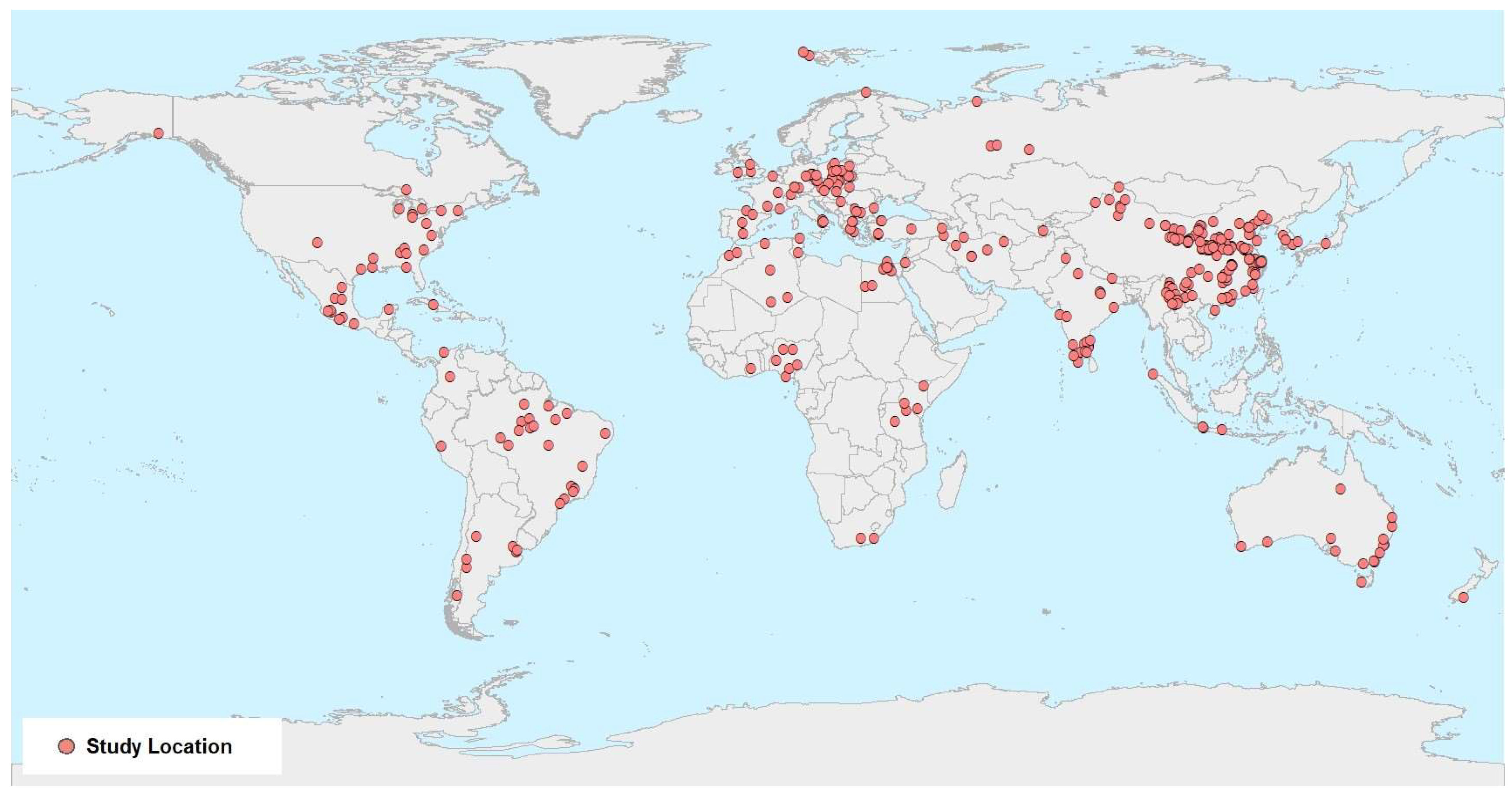
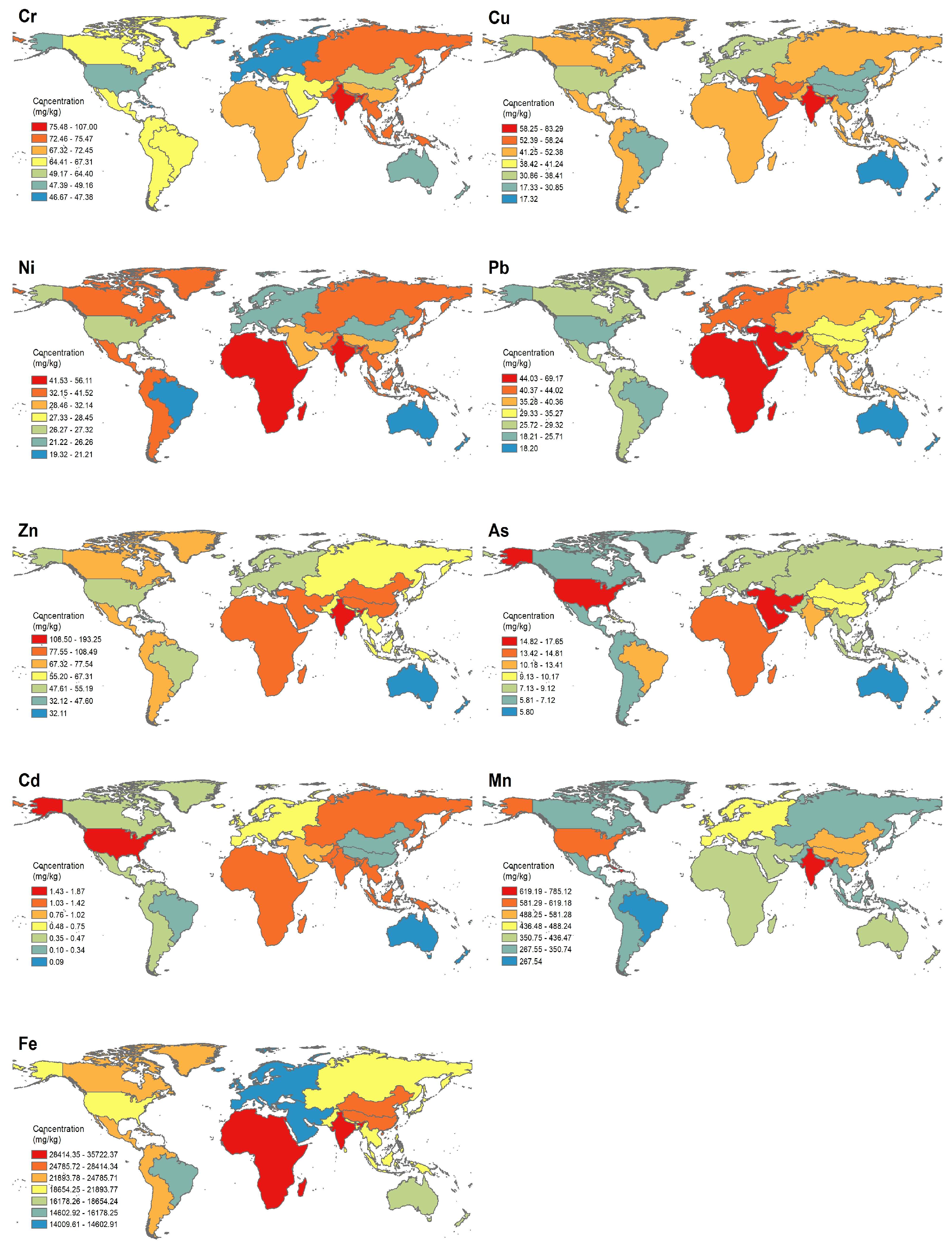
3.1.1. Geographical Distribution Characteristics of HMs

The collected data show the global geographical distribution of HMs as shown in Figure 2. It is particularly noteworthy that HM concentrations in the Indian region are generally higher compared to other countries and regions [68,69,70]. Zn demonstrates minimal variation across different areas, whereas the highest concentrations of Cr, Cu, and Zn are observed in India, corroborating the findings of Adimalla et al. [8]. Additionally, Mn and Ni are present in notably high concentrations in India. Ni and Pb exhibit little regional variation, with the most elevated levels recorded in Africa. In contrast, the United States shows the highest concentrations of Cd and As, aligning with the reports of HM pollution in other scientific literature [4]. Soil HM concentrations in the United States are notably higher compared to other industrially developed regions such as Europe. As a leading global economy, the extensive industrialization and urbanization in the United States have led to substantial industrial and traffic emissions, predominantly involving metals like Pb, Cd, Cr, and Zn [71]. India, currently an emerging economy, is undergoing a period of rapid development. However, in comparison to certain developed countries, India exhibits relative deficiencies in waste treatment and management, leading to an increased influx of HM into the soil [8,72,73]. Consequently, the concentrations of HM in Indian soils are typically elevated, particularly for Zn and Cr, as depicted in Figure 2. The prevalence of HM contamination in India may be partly attributed to inherently high local background levels, often observed in regions with naturally higher concentrations of specific HM in the earth’s crust. India’s crustal background levels are notably higher than in other areas, contributing significantly to the elevated HM concentrations in its soils. Africa, rich in mineral resources, is a key global producer of various metals and minerals. In some African countries, unregulated mining activities, compounded by inadequate local legal and regulatory frameworks, have resulted in elevated concentrations of Pb, Ni, and Cd [74].

Bowen posited that for an element mined more than ten times, its natural cycling rate should be considered a potential environmental pollutant [75]. Consequently, metals like Cd, Cr, Pb, and Zn represent significant ecological risks, as their extraction rates greatly exceed their natural cycling rates. In conclusion, the levels of these HMs vary considerably across different regions, influenced predominantly by a combination of natural background factors, such as soil physicochemical properties, and human activities, including mining, transportation, and industrial and agricultural practices. In addition to natural conditions, the economic structure, social dynamics, and environmental policies of each country and region play crucial roles in determining the types and distribution of HMs in agricultural soils, thereby influencing the accumulation of these metals.

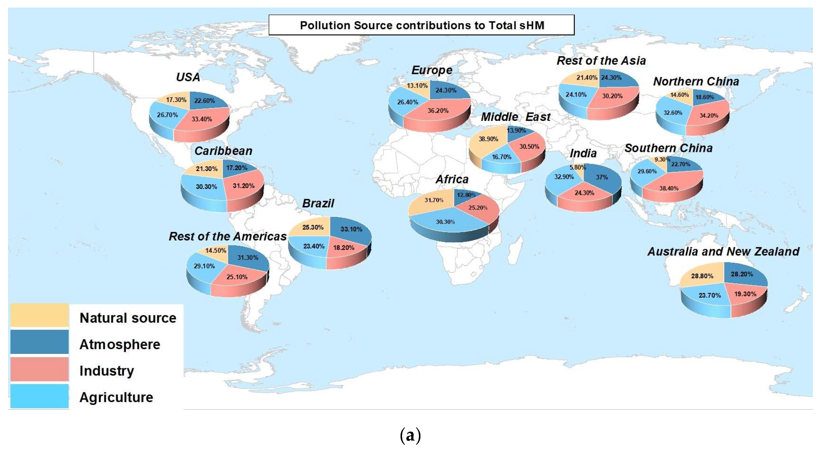
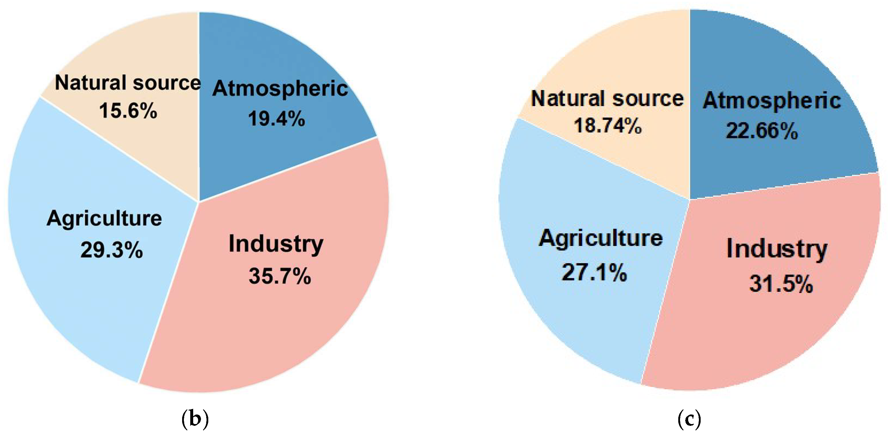
3.1.2. Quantifying the Source Contributions of HMs Using PC-PMF

The predominant sources of HMs are anthropogenic and lithogenic [76]. In order to derive quantitative insights into the contributions of various sources, essential for effective pollution control, we employed the partition-computing-based Positive Matrix Factorization (PC-PMF) model. This approach enabled us to identify the principal sources of HMs and accurately quantify their respective contributions.

The results from each of the 12 sub-datasets in the Positive Matrix Factorization (PMF) receptor model were analyzed, as depicted in Figure 3. The model’s execution and the subsequent analysis of results were guided by methodologies established in prior research [33,46,47,52,77,78]. This study identified four primary emission sources: industrial, agricultural, atmospheric deposition, and natural sources. These sources are known to account for the majority of HM emissions and are distinguishable by their respective metal signatures. Hence, they were chosen as the main contributors to HM emissions. Source identification was corroborated using a multifaceted counterfactual method (referenced in [52]), rather than relying on a single factor. To differentiate between natural and anthropogenic sources of contamination, background soil values specific to each region were employed. Table A1 elaborates on these environmental background values.

The predominant factors for uncontaminated HM emissions are natural sources, which may be further impacted by anthropogenic activities, leading to increased anthropogenic-related emissions. Building on this, our analysis of the 12 sub-datasets identified several potential human-related sources, including local non-ferrous metal industries, agricultural activities, and transportation emissions, as illustrated in Figure 4a. The results indicate the average contributions of various factors to HM emissions across the 12 regions. According to the partition-computing-based Positive Matrix Factorization (PC-PMF) model, industrial activities contribute 31.18% to global HM emissions, followed by agricultural inputs (27.56%), atmospheric deposition (23.16%), and natural sources (18.1%). These findings align with those from the PMF model, as detailed in Figure 4b,c, thereby affirming the PC-PMF model’s accuracy in source apportionment. Nevertheless, the contribution from individual sources varied markedly across different regions. Figure 3 and Figure 4 reveal that in certain regions, industrial activities significantly contribute to HM emissions, predominantly in areas of economic development or rapid growth. Notably, in Europe (36.2%), Southern China (38.4%), Northern China (34.2%), the USA (33.4%), the Caribbean (31.2%), and the Middle East (30.5%), industrial emissions play a substantial role in the contamination of soil and water bodies with HMs. The expansion of industries, particularly in sectors like heavy industry and mining, results in the release of substantial quantities of waste containing toxic HMs, including lead, mercury, cadmium, and arsenic. Agricultural activities are identified as significant contributors to soil pollution in India (32.9%), North China (32.6%), Africa (30.3%), and the Caribbean (30.3%), primarily due to chronic sewage irrigation and inappropriate fertilizer use. In these regions, agricultural irrigation often employs inadequately treated industrial and domestic wastewater, leading to the accumulation of HMs and other hazardous chemicals in the soil [48,49,79]. Furthermore, the excessive or improper application of fertilizers exacerbates soil contamination, particularly with fertilizers containing elements like cadmium, lead, and mercury. This accumulation not only diminishes soil biological activity but also presents a severe risk to crop safety and human health [59,61,80]. The formation of soil matrices, comprising the original materials and processes involved in soil development, is acknowledged as a significant source of HM contamination in soils, notably in Africa (31.7%) and Australia and New Zealand (28.8%). In these regions, soils inherently possess elevated concentrations of HMs, including lead, cadmium, and arsenic. This phenomenon is commonly linked to geological activities, such as volcanic eruptions and rock weathering. These natural processes facilitate the liberation of HMs from the soil matrix, leading to their accumulation in the topsoil [65]. Atmospheric deposition related to transportation has been identified as the principal cause of soil pollution in Brazil (33.1%), India (37%), South America (31.3%), and China (30.1%). The rapid urbanization and escalating number of motor vehicles in these regions contribute to substantial tailpipe emissions [81,82]. These emissions encompass a variety of pollutants, including nitrogen oxides and particulate matter, which, when transported atmospherically, are ultimately deposited in the soil. This process significantly elevates the concentration of hazardous substances in the soil [67]. This increase in national motor vehicle numbers and the escalating issue of tailpipe emissions necessitate targeted interventions.

3.2. Magnetic Parameters

Magnetic susceptibility is a useful proxy for estimating the concentration of ferrimagnetic minerals in soil, as outlined in previous studies. In the data we collected, ${\mathsf{\chi }}_{\mathrm{l}\mathrm{f}}$ varied from 6.45 × 10⁻⁸ m³/kg to 319.23 × 10⁻⁸ m³/kg, with an average value of 72.56 × 10⁻⁸ m³/kg (Figure 5). Meanwhile, the sample standard deviation is 119.21 × 10⁻⁸ m³/kg. The total magnetic susceptibility (${\mathsf{\chi }}_{\mathrm{l}\mathrm{f}}$), encompassing ferrimagnetic, antiferromagnetic, and paramagnetic minerals [21,25,83,84], was observed to be highest in AF, followed by the USA and IN, with ANZ, ME, and ROA1 exhibiting lower levels (Figure 5). The detection of superparamagnetic (SP) particles in soil is inferred from ${\mathsf{\chi }}_{\mathrm{f}\mathrm{d}}$ measurements. The ${\mathsf{\chi }}_{\mathrm{f}\mathrm{d}}$ varied between 0.59% and 12.85%, with an average value of 3.87% and a standard deviation of 5.32%. The highest average value, exceeding 6%, was observed in BR, followed by CA and ME (Figure 5).

Previous research indicates that soil ${\mathsf{\chi }}_{\mathrm{f}\mathrm{d}}$ exceeding 6% suggests a substantial presence of superparamagnetic particles, which are sub-ferromagnetic minerals formed through pedogenesis. A high ${\mathsf{\chi }}_{\mathrm{f}\mathrm{d}}$ generally denotes that the magnetic particles originate predominantly from natural weathering and soil formation processes, with minimal human interference. Conversely, reduced ${\mathsf{\chi }}_{\mathrm{f}\mathrm{d}}$, particularly below 6%, points to a greater influence of human activities on the magnetic particles [24]. In the studies we collected, 76.4% of the samples had ${\mathsf{\chi }}_{\mathrm{f}\mathrm{d}}$ below 6%, signifying that the magnetic particles in these soils are primarily affected by human activities. Soil formation typically produces secondary magnetic minerals, leading to simultaneous increases in ${\mathsf{\chi }}_{\mathrm{l}\mathrm{f}}$ and ${\mathsf{\chi }}_{\mathrm{f}\mathrm{d}}$. Magnetic particles resulting from human activities are often associated with HMs. Nonetheless, it has been proposed that ${\mathsf{\chi }}_{\mathrm{f}\mathrm{d}}$ may decrease in contaminated soils, while ${\mathsf{\chi }}_{\mathrm{l}\mathrm{f}}$ increases [85]. The correlation between ${\mathsf{\chi }}_{\mathrm{l}\mathrm{f}}$ and ${\mathsf{\chi }}_{\mathrm{f}\mathrm{d}}$ in the samples we collected was not substantial (as indicated in Figure 6a), aligning with previous research findings [21,26,28]. Consequently, we suggest that anthropogenic activities may modify the magnetic properties of soil in certain areas without necessarily introducing HM contamination.

3.3. Correlation between Magnetic Susceptibility and HMs

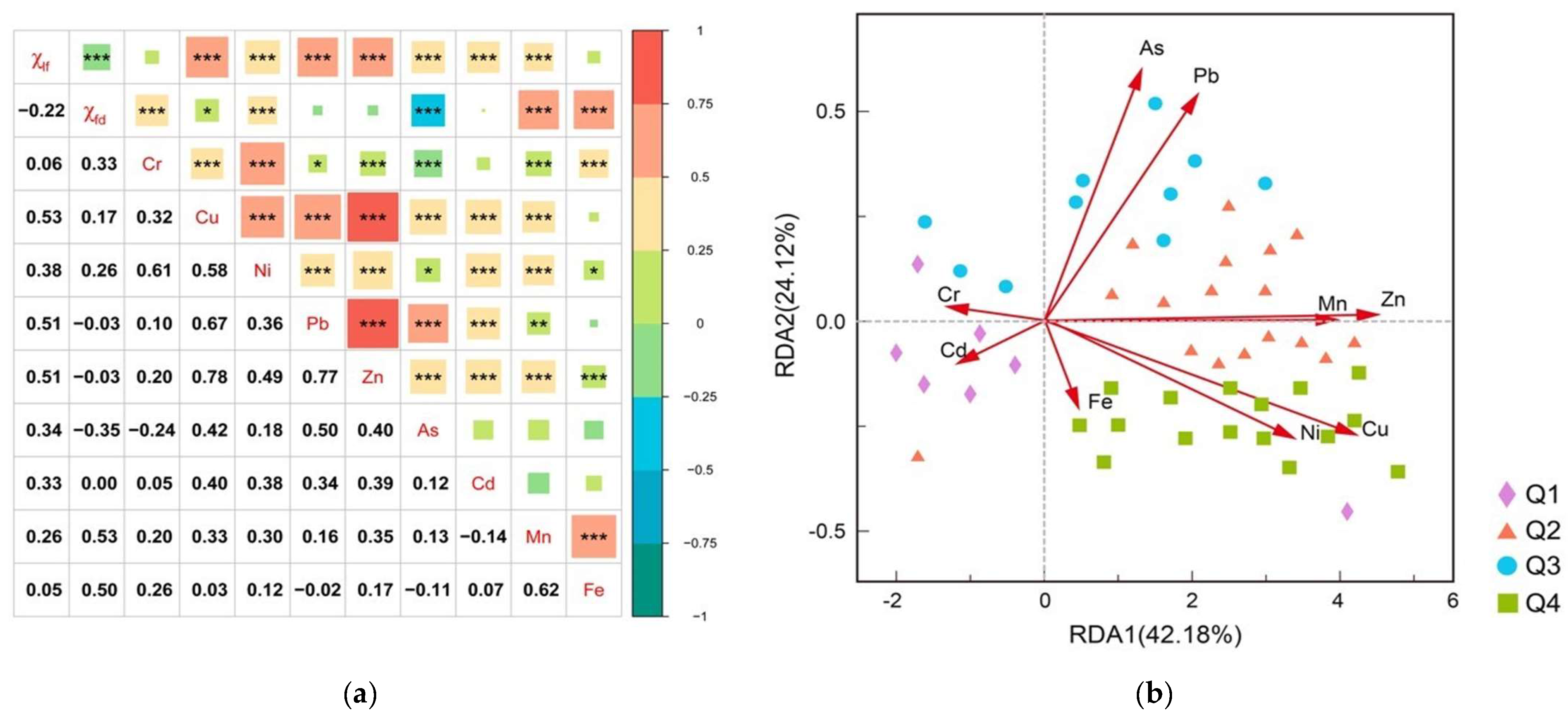
3.3.1. Pearson’s Correlation Analysis

Figure 6a shows Pearson’s correlation coefficient (PCC) between soil HMs and magnetic parameters, revealing a positive correlation across all HMs and ${\mathsf{\chi }}_{\mathrm{l}\mathrm{f}}$. Specifically, a moderate positive correlation was noted with Cu (r = 0.53, p < 0.001), Zn (r = 0.51, p < 0.001), and Pb (r = 0.51, p < 0.001). Ni, As, Cd, and Mn were weakly correlated with ${\mathsf{\chi }}_{\mathrm{l}\mathrm{f}}$ (r of 0.26–0.38, p < 0.001). It can be seen that the ${\mathsf{\chi }}_{\mathrm{l}\mathrm{f}}$ is a potentially effective indicator for the detection of HMs in soil, particularly for Cu, Zn, and Pb. HMs and magnetic minerals can be concurrently enriched in soils through similar geochemical processes, influenced by both natural and anthropogenic factors, resulting in a notable correlation between them, suggesting their coexistence in soils influenced by human activities. The study concludes that the presence of Cu, Zn, and Pb in soil is predominantly due to anthropogenic sources [52,77,78]. The ${\mathsf{\chi }}_{\mathrm{f}\mathrm{d}}$ showed a positive correlation with Fe (r = 0.50, p < 0.001) and Mn (r = 0.53, p < 0.001). The weak correlation between ${\mathsf{\chi }}_{\mathrm{f}\mathrm{d}}$ and HM concentrations implies that these elements are largely from anthropogenic origins. In contrast, a significant positive correlation between ${\mathsf{\chi }}_{\mathrm{f}\mathrm{d}}$ and HMs suggests that these elements predominantly originate from natural soil-forming processes [86,87]. Consequently, the predominant sources of the seven other HMs (Cr, Cu, Zn, Pb, Ni, As, and Cd) in soil are various anthropogenic activities, such as industrial production, motor vehicle exhaust emissions, and agricultural inputs, which generate substantial amounts of magnetic particulate pollutants. Fe and Mn are mainly sourced from natural soil-forming processes [67].

In the correlation analysis of HMs, Zn demonstrated a notably strong positive correlation with Cu (r = 0.78, p < 0.001) and Pb (r = 0.77, p < 0.001). This suggests that Cu, Zn, and Pb share similar geochemical behaviors and contamination sources, primarily linked to transportation. Additionally, there was a significant positive correlation between Cr and Ni (r = 0.61, p < 0.001), as well as between Fe (r = 0.50, p < 0.001) and Mn (r = 0.53, p < 0.001) (Figure 6a), indicating that these metal pairs may originate from similar sources. In contrast, other HMs showed weaker or no correlations, pointing to different sources of contamination. It is crucial to recognize that the interactions among HMs are intricate and influenced by a multitude of factors; therefore, Pearson’s coefficient alone may not yield a comprehensive understanding of these relationships [57].

3.3.2. Redundancy Analysis

In order to further understand the association between ${\mathsf{\chi }}_{\mathrm{l}\mathrm{f}}$ intensity and HM concentrations at different sampling points, the ${\mathsf{\chi }}_{\mathrm{l}\mathrm{f}}$ intensity as a function of indicator variables was investigated using the statistical method redundancy analysis (RDA). In this study, the main comparative analysis was used to classify the soil ${\mathsf{\chi }}_{\mathrm{l}\mathrm{f}}$ sampling sites into four groups based on the quartile method, Q1, Q2, Q3, and Q4, to investigate the indicative roles of the sampling sites with different ${\mathsf{\chi }}_{\mathrm{l}\mathrm{f}}$ intensities in the accumulation of HMs. The results of the RDA showed that the elements of Pb, Zn, Cu, and As were the key factors that contributed to the differences in the response of the different intensities of the ${\mathsf{\chi }}_{\mathrm{l}\mathrm{f}}$ (Figure 6b). The first and second axes explained 42.18% and 24.12% of the variance of the four subgroups, respectively (Figure 6b). The positive correlation between Ni and Cu at the Q4 sampling site, along with the acute angle between the Q3 sampling site and both Pb and As, suggests that Pb, As, and Cu significantly affect the magnetic response of sites Q3 and Q4. This pattern indicates that the Q3 and Q4 sites likely experience substantial industrial and mining activities. Conversely, the Q2 sampling site, being close to Zn and forming an obtuse angle with other metals, reveals that Zn notably influences the magnetic response at this location. The prevalence of Q2 sites in agricultural countries hints at severe agricultural pollution. Furthermore, the correlation matrix shows a strong association of ${\mathsf{\chi }}_{\mathrm{l}\mathrm{f}}$ with Pb, Zn, and Cu, confirming the metals present at the Q2, Q3, and Q4 sampling points are highly sensitive to the ${\mathsf{\chi }}_{\mathrm{l}\mathrm{f}}$. Similarly, the Q1 sampling site is observed to have a positive correlation with both chromium Cr and Cd and lies proximate to Fe. Considering the negligible correlation between Fe and ${\mathsf{\chi }}_{\mathrm{l}\mathrm{f}}$ as presented in Figure 6a and the fact that the majority of soil Fe(H) oxides possess weak magnetic properties (being either antiferromagnetic or paramagnetic), it is likely that the Fe observed here primarily originates from soil-forming processes rather than anthropogenic sources. In general, the ferromagnetic form accounts for a lower content in soils, typically less than 1% [66], reinforcing the pedogenetic perspective of Fe’s presence in these sampling sites. These observations suggest that the enhanced accumulation of Cr and Cd at the Q1 sampling points can be ascribed to natural soil composition rather than industrial contributions. This implies that the spatial distribution of certain heavy metals is largely influenced by the underlying geological matrix, reiterating the natural origin of Cr and Cd in the Q1 site as shown in Figure 6b.

3.4. Magnetic Susceptibility Indicates HM Contamination

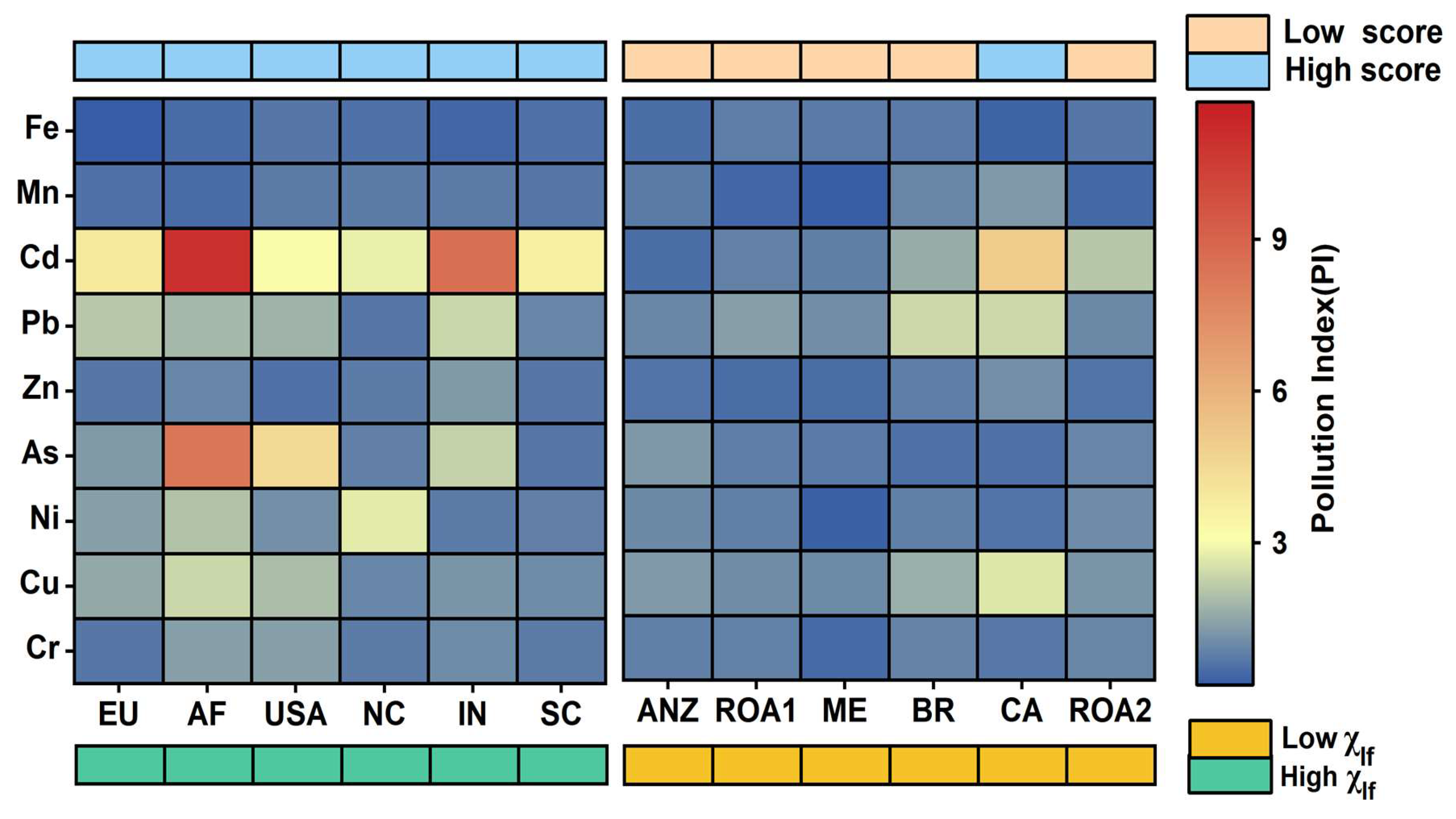
3.4.1. Evaluation of Pollution Indices of HMs

The pollution index (PI = CF) and pollution load index (PLI) regression analyses were employed to assess HM pollution across 12 regions (Figure 7). We divided the regions into two groups and noticed a significant difference in CF values between areas with high ${\mathsf{\chi }}_{\mathrm{l}\mathrm{f}}$ (Q3–Q4) and low ${\mathsf{\chi }}_{\mathrm{l}\mathrm{f}}$ (Q1–Q2). Generally, regions with high PI scores corresponded to high ${\mathsf{\chi }}_{\mathrm{l}\mathrm{f}}$ (Q3~Q4), except for CA. Regions such as the EU, AF, USA, NC, IN, CA, and SC exhibited high CF scores, ranging from 1.62 to 3.41, with an average of 2.69 (the standard deviation is 0.58), correlating with high ${\mathsf{\chi }}_{\mathrm{l}\mathrm{f}}$ and indicating substantial HM enrichment. This suggests a considerable ecological risk, primarily attributed to Cd, As, and Cu (Figure 7). Notably, three communities had CF values above 2, indicative of moderate pollution, while AF’s average CF value exceeded 3, signaling poor soil quality and severe HM risk. In contrast, ANZ, ROA1, ME, BR, and ROA2 formed low-scoring communities, with CF scores between 0.93 and 1.53 and an average of 1.24 (the standard deviation is 0.23), denoting mild pollution.

Our findings reveal moderate artificial enrichment of Cr (average CF = 1.53) and Cu (average CF = 1.98) in soil, whereas Cd (average CF = 3.61), Pb (average CF = 2.27), and As (average CF = 2.32) exhibit significantly higher enrichment. The pollution load index (PLI) for five metal elements exhibited an average value of 2.03 (the standard deviation is 0.77), which signifies a moderate degree of agricultural soil contamination on a global scale [64,65]. Among various HM contaminants, Cd demonstrates the most significant enrichment (Figure 7). This accumulation in the environment poses a considerable threat to ecosystems and adversely impacts human health. In regions with significant industrial contributions, such as the EU, IN, SC, and the USA, elevated CF values of Cd, As, Pb, and Cu were noted. The origin of these HMs can be traced to human activities like non-ferrous metal processing, mining, smelting, and agricultural inputs. It is worth mentioning that in Africa, cadmium levels are highly localized due to mining, road traffic, and agricultural additives. However, besides such human activities leading to elevated magnetic susceptibility (Q3~Q4), the pedogenesis of tropical soils in Africa is also a significant factor. For instance, in tropical regions of Africa, iron primarily exists in the form of laterites with high microbial activity, which may increase the abundance of superparamagnetic particles, consequently resulting in higher soil magnetic susceptibility values [74]. Therefore, future research should delve deeper into the specific impacts of these pedogenic processes on magnetic susceptibility, for a more accurate understanding and assessment of the relationship between magnetic response and heavy metal pollution. This will contribute to enhancing the precision of studies and specific applications in geographical regions.

3.4.2. Regression Analysis of PLI and ${\mathsf{\chi }}_{\mathrm{l}\mathrm{f}}$

Figure 8 presents the segmented linear regression model linking log-normal magnetic susceptibility with the pollution index (CF). At the threshold of ${\mathrm{l}\mathrm{n}\mathsf{\chi }}_{\mathrm{l}\mathrm{f}}$ = 3.26 or ${\mathsf{\chi }}_{\mathrm{l}\mathrm{f}}=26\times {10}^{-8}{\mathrm{m}}^3/\mathrm{k}\mathrm{g}$, the CF values for all HMs remain stable. However, above specific thresholds—3.26 ${\mathsf{\chi }}_{\mathrm{l}\mathrm{f}}>43\times {10}^{-8} {\mathrm{m}}^3/\mathrm{k}\mathrm{g} ({\mathrm{l}\mathrm{n}\mathsf{\chi }}_{\mathrm{l}\mathrm{f}}>3.78)$ for Cd, ${\mathsf{\chi }}_{\mathrm{l}\mathrm{f}}>26\times {10}^{-8}{\mathrm{m}}^3/\mathrm{k}\mathrm{g} ({\mathrm{l}\mathrm{n}\mathsf{\chi }}_{\mathrm{l}\mathrm{f}}>3.26)$ for Cr, ${\mathsf{\chi }}_{\mathrm{l}\mathrm{f}}>37\times {10}^{-8}{\mathrm{m}}^3/\mathrm{k}\mathrm{g}$ $({\mathrm{l}\mathrm{n}\mathsf{\chi }}_{\mathrm{l}\mathrm{f}}>3.61)$ for Cu, and ${\mathsf{\chi }}_{\mathrm{l}\mathrm{f}}>28\times {10}^{-8}{\mathrm{m}}^3/\mathrm{k}\mathrm{g} ({\mathrm{l}\mathrm{n}\mathsf{\chi }}_{\mathrm{l}\mathrm{f}}>3.32)$ for Pb and As—the correlation between CF and logarithmic ${\mathsf{\chi }}_{\mathrm{l}\mathrm{f}}$ becomes significant (see

Table 4. Piecewise function regression mathematical diagnostic model.

HM	$\mathbf{B}\mathbf{P}\mathbf{i}$	${\mathsf{\chi }}_{\mathbf{l}\mathbf{f}}$ Thresholds	Regression Equation	Correlation Coefficient
Cd	3.78	43	${\mathrm{CF}}_{\mathrm{Cd}}=0.63\ln ({\mathsf{\chi }}_{\mathrm{l}\mathrm{f}}$) − 0.23	0.673
Cr	3.26	26	${\mathrm{CF}}_{\mathrm{Cr}}=0.67\ln ({\mathsf{\chi }}_{\mathrm{l}\mathrm{f}}$) − 2.52	0.556
Cu	3.61	37	${\mathrm{CF}}_{\mathrm{Cu}}=1.24\ln ({\mathsf{\chi }}_{\mathrm{l}\mathrm{f}}$) − 1.31	0.571
Pb	3.32	28	${\mathrm{CF}}_{\mathrm{Pb}}=0.93\ln ({\mathsf{\chi }}_{\mathrm{l}\mathrm{f}}$) − 0.98	0.467
As	3.32	28	${\mathrm{CF}}_{\mathrm{As}}=0.57\ln ({\mathsf{\chi }}_{\mathrm{l}\mathrm{f}}$) + 1.21	0.483
PLI	3.26	-	$\mathrm{PLI}=0.81\ln ({\mathsf{\chi }}_{\mathrm{l}\mathrm{f}}$) − 0.83	0.721

and Figure 8). For ${\mathsf{\chi }}_{\mathrm{l}\mathrm{f}}=26\times {10}^{-8} {\mathrm{m}}^3/\mathrm{k}\mathrm{g} ({\mathrm{l}\mathrm{n}\mathsf{\chi }}_{\mathrm{l}\mathrm{f}}=3.26)$, HM concentrations in soil approximate natural background levels or indicate low pollution. Conversely, a threshold of ${\mathsf{\chi }}_{\mathrm{l}\mathrm{f}}=26\times {10}^{-8} {\mathrm{m}}^3/\mathrm{k}\mathrm{g}$ may distinguish soil layers with natural HM content from those artificially enriched with magnetic particles and trace metals (${\mathsf{\chi }}_{\mathrm{l}\mathrm{f}}>26\times {10}^{-8} {\mathrm{m}}^3/\mathrm{k}\mathrm{g}$). For samples exceeding this threshold, all CFs show a significant positive correlation (r = 0.489–0.673, p < 0.001, Figure 8), although deviations from the fitted confidence intervals are noted for individual HMs (Figure 8).

In fact, the magnetic diagnostic criteria for heavy metal pollution in agricultural soil are only qualitative (semi-quantitative) standards. The determination coefficients of the magnetic diagnostic model for pollution factors and the pollution load index (PLI) range from 0.467 to 0.721, indicating a certain level of error inherent in the model itself [88]. In soil magnetism studies, human interventions and land management practices like plowing, irrigation, earthworks, and construction can redistribute magnetic particles in the soil, potentially obscuring the correlation between ${\mathsf{\chi }}_{\mathrm{l}\mathrm{f}}$ and surface soil HM concentration [19]. This redistribution underlines the significant impact of anthropogenic activities and soil disturbance on the soil’s physical and chemical properties. Moreover, the extent of the correlation between ${\mathsf{\chi }}_{\mathrm{l}\mathrm{f}}$ and specific HMs provides insights into soil contamination sources. For instance, the correlation coefficient (r = 0.673) between CF_Cd and logarithmic susceptibility indicates that 67.3% of Cd variability is attributable to human factors [85]. Similarly, the variability of Cr (r = 0.556), Cu (r = 0.571), Pb (r = 0.489), and As (r = 0.527) is respectively associated with anthropogenic influences, accounting for 55.6%, 57.1%, 48.9%, and 52.7% of their variability. This link to human activities is corroborated by the pollution load index (PLI) with an r of 0.721 (Figure 8), suggesting that the PLI can explain approximately 72% of ${\mathsf{\chi }}_{\mathrm{l}\mathrm{f}}$ variation and is indicative of the total HM pollution load (r = 0.72) [58,65]. More specifically, correlating perceived ${\mathsf{\chi }}_{\mathrm{l}\mathrm{f}}$ with geochemical soil properties enables the identification of variations in anthropogenic activities and soil lithology. Elevated ${\mathsf{\chi }}_{\mathrm{l}\mathrm{f}}$ suggests a higher concentration of magnetic materials in the soil, which may indicate potential contamination sources. To accurately assess pollution, one can initially use the magnetic susceptibility measurement method, followed by measuring other magnetic parameters for evaluation [27,89]. This understanding aids in discerning the nature of human impacts, such as from non-ferrous metal smelting and traffic emissions. Although ${\mathsf{\chi }}_{\mathrm{l}\mathrm{f}}$ cannot quantify specific metal contamination, it is useful for identifying areas with relatively high HM contamination. This technique can be utilized in other urban areas to evaluate the overall environmental impact on soil communities. Furthermore, it offers a rapid and sensitive approach for assessing soil quality over extensive areas. These findings further solidify ${\mathsf{\chi }}_{\mathrm{l}\mathrm{f}}$ as a critical indicator in soil environmental research.

4. Conclusions

This study synthesized global heavy metal and magnetic susceptibility data, conducting a systematic meta-analysis to explore the geographical distribution of agricultural soil heavy metal contents and their magnetic susceptibility, along with quantitative source analysis of the heavy metals. Finally, a comprehensive analysis was conducted to explore the correlation between magnetic susceptibility and HM contamination in agricultural soils. The results are as follows:

• There are significant regional differences in the global distribution of HMs, which are relatively high in India, the USA, Africa, etc. Additionally, the PC-PMF model reveals global variations in pollution sources, with the industry being the primary contributor (31.5%). Effective soil management policies can be formulated by considering regional variations in source contributions.
• The total magnetic concentration of the agricultural soils in different regions varied significantly, and the ${\mathsf{\chi }}_{\mathrm{f}\mathrm{d}}$ ranged from 0.59% and 12.85%, with the majority of the samples being below 6%, suggesting that magnetic particles in the soils are mainly influenced by human activities.
• Pearson’s correlation analysis showed that soil magnetic susceptibility was significantly and positively correlated with specific heavy metals, such as Pb, Zn, and Cu with ${\mathsf{\chi }}_{\mathrm{l}\mathrm{f}}$ (r = 0.51–0.53) and Mn and Fe with ${\mathsf{\chi }}_{\mathrm{f}\mathrm{d}}$ (r = 0.50–0.53), and combined with the RDA analysis, it was determined that Pb, Zn, Cu, and As were the key factors influencing the differences in soil magnetic response.
• The global agricultural soil HM contamination assessment indicated a moderate level of soil contamination, with a PLI of 2.03. A significant positive correlation was observed between magnetic susceptibility (${\mathsf{\chi }}_{\mathrm{l}\mathrm{f}}$) above $26\times {10}^{-8} {\mathrm{m}}^3/\mathrm{k}\mathrm{g}$ and both heavy metal concentration and the PLI (r = 0.72), affirming ${\mathsf{\chi }}_{\mathrm{l}\mathrm{f}}$ as a robust predictor of HM contamination. These insights are crucial for developing effective soil management strategies and conducting large-scale soil quality assessments.

References

1. Solgi, E.; Esmaili-Sari, A.; Riyahi-Bakhtiari, A.; Hadipour, M. Soil Contamination of Metals in the Three Industrial Estates, Arak, Iran. Bull. Environ. Contam. Toxicol. 2012, 88, 634–638. [Google Scholar] [CrossRef] [PubMed]
2. Shi, T.; Ma, J.; Zhang, Y.; Liu, C.; Hu, Y.; Gong, Y.; Wu, X.; Ju, T.; Hou, H.; Zhao, L. Status of Lead Accumulation in Agricultural Soils across China (1979–2016). Environ. Int. 2019, 129, 35–41. [Google Scholar] [CrossRef] [PubMed]
3. Liu, P.; Hu, W.; Tian, K.; Huang, B.; Zhao, Y.; Wang, X.; Zhou, Y.; Shi, B.; Kwon, B.-O.; Choi, K.; et al. Accumulation and Ecological Risk of Heavy Metals in Soils along the Coastal Areas of the Bohai Sea and the Yellow Sea: A Comparative Study of China and South Korea. Environ. Int. 2020, 137, 105519. [Google Scholar] [CrossRef] [PubMed]
4. Han, I.; Whitworth, K.W.; Christensen, B.; Afshar, M.; An Han, H.; Rammah, A.; Oluwadairo, T.; Symanski, E. Heavy Metal Pollution of Soils and Risk Assessment in Houston, Texas Following Hurricane Harvey. Environ. Pollut. 2022, 296, 118717. [Google Scholar] [CrossRef] [PubMed]
5. Reimann, C.; De Caritat, P. New Soil Composition Data for Europe and Australia: Demonstrating Comparability, Identifying Continental-Scale Processes and Learning Lessons for Global Geochemical Mapping. Sci. Total Environ. 2012, 416, 239–252. [Google Scholar] [CrossRef] [PubMed]
6. Tao, H.; Al-Hilali, A.A.; Ahmed, A.M.; Mussa, Z.H.; Falah, M.W.; Abed, S.A.; Deo, R.; Jawad, A.H.; Abdul Maulud, K.N.; Latif, M.T.; et al. Statistical and Spatial Analysis for Soil Heavy Metals over the Murray-Darling River Basin in Australia. Chemosphere 2023, 317, 137914. [Google Scholar] [CrossRef] [PubMed]
7. Huang, Y.; Wang, L.; Wang, W.; Li, T.; He, Z.; Yang, X. Current Status of Agricultural Soil Pollution by Heavy Metals in China: A Meta-Analysis. Sci. Total Environ. 2019, 651, 3034–3042. [Google Scholar] [CrossRef] [PubMed]
8. Adimalla, N.; Qian, H.; Wang, H. Assessment of Heavy Metal (HM) Contamination in Agricultural Soil Lands in Northern Telangana, India: An Approach of Spatial Distribution and Multivariate Statistical Analysis. Environ. Monit. Assess. 2019, 191, 246. [Google Scholar] [CrossRef]
9. Zang, F.; Wang, S.; Nan, Z.; Ma, J.; Zhang, Q.; Chen, Y.; Li, Y. Accumulation, Spatio-Temporal Distribution, and Risk Assessment of Heavy Metals in the Soil-Corn System around a Polymetallic Mining Area from the Loess Plateau, Northwest China. Geoderma 2017, 305, 188–196. [Google Scholar] [CrossRef]
10. Huamain, C.; Chunrong, Z.; Cong, T.; Yongguan, Z. Heavy Metal Pollution in Soils in China: Status and Countermeasures. Ambio 1999, 28, 130–134. [Google Scholar]
11. Imseng, M.; Wiggenhauser, M.; Müller, M.; Keller, A.; Frossard, E.; Wilcke, W.; Bigalke, M. The Fate of Zn in Agricultural Soils: A Stable Isotope Approach to Anthropogenic Impact, Soil Formation, and Soil–Plant Cycling. Environ. Sci. Technol. 2019, 53, 4140–4149. [Google Scholar] [CrossRef] [PubMed]
12. Beone, G.M.; Carini, F.; Guidotti, L.; Rossi, R.; Gatti, M.; Fontanella, M.C.; Cenci, R.M. Potentially toxic elements in agricultural soils from the Lombardia region of northern Italy. J. Geochem. Explor. 2018, 190, 436–452. [Google Scholar] [CrossRef]
13. Morton-Bermea, O.; Hernandez, E.; Martinez-Pichardo, E.; Soler-Arechalde, A.M.; Santa-Cruz, R.L.; Gonzalez-Hernandez, G.; Beramendi-Orosco, L.; Urrutia-Fucugauchi, J. Mexico City Topsoils: Heavy Metals vs. Magnetic Susceptibility. Geoderma 2009, 151, 121–125. [Google Scholar] [CrossRef]
14. Yin, Y.; Wang, X.; Hu, Y.; Li, F.; Cheng, H. Soil Bacterial Community Structure in the Habitats with Different Levels of Heavy Metal Pollution at an Abandoned Polymetallic Mine. J. Hazard. Mater. 2023, 442, 130063. [Google Scholar] [CrossRef] [PubMed]
15. Alloway, B.J. Sources of heavy metals and metalloids in soils. In Heavy Metals in Soils: Trace Metals and Metalloids in Soils and Their Bioavailability; Alloway, B.J., Ed.; Springer: Berlin/Heidelberg, Germany, 1995; pp. 11–50. [Google Scholar]
16. Abel, S.; Nehls, T.; Mekiffer, B.; Mathes, M.; Thieme, J.; Wessolek, G. Pools of Sulfur in Urban Rubble Soils. J. Soils Sediments 2015, 15, 532–540. [Google Scholar] [CrossRef]
17. Hoefs, J. Geochemical Fingerprints: A Critical Appraisal. Eur. J. Mineral. 2010, 22, 3–15. [Google Scholar] [CrossRef]
18. Erosion, I. Geochemistry in soil science. In Encyclopedia of Soil Science; Springer: Berlin/Heidelberg, Germany, 2007; p. 283. ISBN 978-1-4020-3994-2. [Google Scholar]
19. Delbecque, N.; Van Ranst, E.; Dondeyne, S.; Mouazen, A.M.; Vermeir, P.; Verdoodt, A. Geochemical Fingerprinting and Magnetic Susceptibility to Unravel the Heterogeneous Composition of Urban Soils. Sci. Total Environ. 2022, 847, 157502. [Google Scholar] [CrossRef]
20. Verosub, K.L.; Roberts, A.P. Environmental Magnetism: Past, Present, and Future. J. Geophys. Res. 1995, 100, 2175–2192. [Google Scholar] [CrossRef]
21. Vodyanitskii, Y.N.; Shoba, S.A. Magnetic Susceptibility as an Indicator of Heavy Metal Contamination of Urban Soils (Review). Moscow Univ. Soil Sci. Bull. 2015, 70, 10–16. [Google Scholar] [CrossRef]
22. Vollprecht, D.; Bobe, C.; Stiegler, R.; Van De Vijver, E.; Wolfsberger, T.; Küppers, B.; Scholger, R. Relating magnetic properties of municipal solid waste constituents to iron content: Implications for enhanced landfill mining. Detritus 2019, 8, 31–46. [Google Scholar] [CrossRef]
23. Magiera, T.; Żogała, B.; Łukasik, A.; Pierwoła, J. Application of Different Geophysical Techniques to Study Technosol Developed on Metallurgical Wastes. Land Degrad. Dev. 2021, 32, 1927–1937. [Google Scholar] [CrossRef]
24. Karimi, R.; Ayoubi, S.; Jalalian, A.; Sheikh-Hosseini, A.R.; Afyuni, M. Relationships between Magnetic Susceptibility and Heavy Metals in Urban Topsoils in the Arid Region of Isfahan, Central Iran. J. Appl. Geophys. 2011, 74, 1–7. [Google Scholar] [CrossRef]
25. Ayoubi, S.; Karami, M. Pedotransfer functions for predicting heavy metals in natural soils using magnetic measures and soil properties. J. Geochem. Explor. 2019, 197, 212–219. [Google Scholar] [CrossRef]
26. Gargiulo, J.D.; Chaparro, M.A.; Marié, D.C.; Böhnel, H.N. Magnetic monitoring of anthropogenic pollution in Antarctic soils (Marambio Station) and the spatial-temporal changes over a decade. Catena 2021, 203, 105289. [Google Scholar] [CrossRef]
27. Chaparro, M.A.; Suresh, G.; Chaparro, M.A.; Ramasamy, V.; Sundarrajan, M. Magnetic assessment and pollution status of beach sediments from Kerala coast (southwestern India). Mar. Pollut. Bull. 2017, 117, 171–177. [Google Scholar] [CrossRef] [PubMed]
28. Joju, G.S.; Warrier, A.K.; Sali, A.Y.; Chaparro, M.A.; Mahesh, B.S.; K, A.; Mohan, R. An Assessment of Metal Pollution in the Surface Sediments of an East Antarctic Lake. Soil Sediment Contam. Int. J. 2024, 1–22. [Google Scholar] [CrossRef]
29. El Baghdadi, M.; Barakat, A.; Sajieddine, M.; Nadem, S. Heavy Metal Pollution and Soil Magnetic Susceptibility in Urban Soil of Beni Mellal City (Morocco). Environ. Earth Sci. 2012, 66, 141–155. [Google Scholar] [CrossRef]
30. Canbay, M.; Aydin, A.; Kurtulus, C. Magnetic Susceptibility and Heavy-Metal Contamination in Topsoils along the Izmit Gulf Coastal Area and IZAYTAS (Turkey). J. Appl. Geophys. 2010, 70, 46–57. [Google Scholar] [CrossRef]
31. Gubbins, D.; Herrero-Bervera, E. (Eds.) Encyclopedia of Geomagnetism and Paleomagnetism; Springer Science & Business Media: Berlin/Heidelberg, Germany, 2007; pp. 1–1013. ISBN 978-1-4020-3992-8. [Google Scholar]
32. Łukasik, A.; Szuszkiewicz, M.; Magiera, T. Impact of Artifacts on Topsoil Magnetic Susceptibility Enhancement in Urban Parks of the Upper Silesian Conurbation Datasets. J. Soils Sediments 2015, 15, 1836–1846. [Google Scholar] [CrossRef]
33. Wang, B.; Xia, D.; Yu, Y.; Chen, H.; Jia, J. Source Apportionment of Soil-Contamination in Baotou City (North China) Based on a Combined Magnetic and Geochemical Approach. Sci. Total Environ. 2018, 642, 95–104. [Google Scholar] [CrossRef]
34. Szuszkiewicz, M.; Łukasik, A.; Magiera, T.; Mendakiewicz, M. Combination of geo-pedo-and technogenic magnetic and geochemical signals in soil profiles–diversification and its interpretation: A new approach. Environ. Pollut. 2016, 214, 464–477. [Google Scholar] [CrossRef] [PubMed]
35. Cao, L.; Appel, E.; Hu, S.; Ma, M. An Economic Passive Sampling Method to Detect Particulate Pollutants Using Magnetic Measurements. Environ. Pollut. 2015, 205, 97–102. [Google Scholar] [CrossRef] [PubMed]
36. Prajith, A.; Rao, V.P.; Kessarkar, P.M. Magnetic Properties of Sediments in Cores from the Mandovi Estuary, Western India: Inferences on Provenance and Pollution. Mar. Pollut. Bull. 2015, 99, 338–345. [Google Scholar] [CrossRef] [PubMed]
37. Pan, H.; Lu, X.; Lei, K.; Shi, D.; Ren, C.; Yang, L.; Wang, L. Using Magnetic Susceptibility to Evaluate Pollution Status of the Sediment for a Typical Reservoir in Northwestern China. Environ. Sci. Pollut. Res. 2019, 26, 3019–3032. [Google Scholar] [CrossRef] [PubMed]
38. Hu, P.; Heslop, D.; Viscarra Rossel, R.A.; Roberts, A.P.; Zhao, X. Continental-Scale Magnetic Properties of Surficial Australian Soils. Earth-Sci. Rev. 2020, 203, 103028. [Google Scholar] [CrossRef]
39. Hannam, J.A.; Dearing, J.A. Mapping Soil Magnetic Properties in Bosnia and Herzegovina for Landmine Clearance Operations. Earth Planet. Sci. Lett. 2008, 274, 285–294. [Google Scholar] [CrossRef]
40. Johansson, C.; Norman, M.; Burman, L. Road Traffic Emission Factors for Heavy Metals. Atmos. Environ. 2009, 43, 4681–4688. [Google Scholar] [CrossRef]
41. Jordanova, N.; Jordanova, D.; Petrov, P. Soil Magnetic Properties in Bulgaria at a National Scale—Challenges and Benefits. Glob. Planet. Chang. 2016, 137, 107–122. [Google Scholar] [CrossRef]
42. Thiesson, J.; Boulonne, L.; Buvat, S.; Jolivet, C.; Ortolland, B.; Saby, N. Magnetic Properties of the French Soil Monitoring Network: First Results; European Association of Geoscientists & Engineers: Utrecht, The Netherlands, 2012; pp. 1–306. [Google Scholar]
43. Hanesch, M.; Rantitsch, G.; Hemetsberger, S.; Scholger, R. Erratum to “Lithological and Pedological Influences on the Magnetic Susceptibility of Soil: Their Consideration in Magnetic Pollution Mapping [Science of the Total Environment 382 (2007) 351–363]”. Sci. Total Environ. 2008, 396, 86–87. [Google Scholar] [CrossRef]
44. Chaparro, M.A.; Nuñez, H.; Lirio, J.M.; Gogorza, C.S.; Sinito, A.M. Magnetic screening and heavy metal pollution studies in soils from Marambio Station, Antarctica. Antarct. Sci. 2007, 19, 379–393. [Google Scholar] [CrossRef]
45. Chaparro, M.A.; Chaparro, M.A.; Molinari, D.A. A Fuzzy-Based Analysis of Air Particle Pollution Data: An Index IMC for Magnetic Biomonitoring. Atmosphere 2024, 15, 435. [Google Scholar] [CrossRef]
46. Ma, W.; Tai, L.; Qiao, Z.; Zhong, L.; Wang, Z.; Fu, K.; Chen, G. Contamination Source Apportionment and Health Risk Assessment of Heavy Metals in Soil around Municipal Solid Waste Incinerator: A Case Study in North China. Sci. Total Environ. 2018, 631–632, 348–357. [Google Scholar] [CrossRef]
47. Schaefer, K.; Einax, J.W. Source Apportionment and Geostatistics: An Outstanding Combination for Describing Metals Distribution in Soil. CLEAN Soil Air Water 2016, 44, 877–884. [Google Scholar] [CrossRef]
48. Dong, B.; Zhang, R.; Gan, Y.; Cai, L.; Freidenreich, A.; Wang, K.; Guo, T.; Wang, H. Multiple Methods for the Identification of Heavy Metal Sources in Cropland Soils from a Resource-Based Region. Sci. Total Environ. 2019, 651, 3127–3138. [Google Scholar] [CrossRef]
49. Zhou, L.; Zhao, X.; Meng, Y.; Fei, Y.; Teng, M.; Song, F.; Wu, F. Identification Priority Source of Soil Heavy Metals Pollution Based on Source-Specific Ecological and Human Health Risk Analysis in a Typical Smelting and Mining Region of South China. Ecotoxicol. Environ. Saf. 2022, 242, 113864. [Google Scholar] [CrossRef]
50. Feng, Y.-X.; Yu, X.-Z.; Zhang, H. A Modelling Study of a Buffer Zone in Abating Heavy Metal Contamination from a Gold Mine of Hainan Province in Nearby Agricultural Area. J. Environ. Manag. 2021, 287, 112299. [Google Scholar] [CrossRef]
51. Liu, P.; Hu, W.; Huang, B.; Liu, B.; Zhou, Y. Advancement in researches on effect of atmospheric deposition on heavy metals accumulation in soils and crops. Acta Pedol. Sin. 2019, 565, 1048–1059. [Google Scholar] [CrossRef]
52. Wu, J.; Li, J.; Teng, Y.; Chen, H.; Wang, Y. A Partition Computing-Based Positive Matrix Factorization (PC-PMF) Approach for the Source Apportionment of Agricultural Soil Heavy Metal Contents and Associated Health Risks. J. Hazard. Mater. 2020, 388, 121766. [Google Scholar] [CrossRef]
53. UNSD. Standard Country or Area Codes for Statistical Use (M49). 2023. Available online: https://unstats.un.org/unsd/methodology/m49/ (accessed on 14 October 2023).
54. Paatero, P.; Tapper, U. Positive Matrix Factorization: A Non-negative Factor Model with Optimal Utilization of Error Estimates of Data Values. Environmetrics 1994, 5, 111–126. [Google Scholar] [CrossRef]
55. Brown, S.G.; Eberly, S.; Paatero, P.; Norris, G.A. Methods for Estimating Uncertainty in PMF Solutions: Examples with Ambient Air and Water Quality Data and Guidance on Reporting PMF Results. Sci. Total Environ. 2015, 518–519, 626–635. [Google Scholar] [CrossRef]
56. Armstrong, R.A. Should Pearson’s correlation coefficient be avoided? Ophthalmic Physiol. Opt. 2019, 39, 316–327. [Google Scholar] [CrossRef]
57. Łukasik, A.; Magiera, T.; Lasota, J.; Błońska, E. Background Value of Magnetic Susceptibility in Forest Topsoil: Assessment on the Basis of Studies Conducted in Forest Preserves of Poland. Geoderma 2016, 264, 140–149. [Google Scholar] [CrossRef]
58. Deng, L.; Fan, Y.; Liu, K.; Zhang, Y.; Qian, X.; Li, M.; Wang, S.; Xu, X.; Gao, X.; Li, H. Exploring the primary magnetic parameters affecting chemical fractions of heavy metal (loid) s in lake sediment through an interpretable workflow. J. Hazard. Mater. 2024, 468, 133859. [Google Scholar] [CrossRef]
59. Lin, Y.; Han, P.; Huang, Y.; Yuan, G.L.; Guo, J.X.; Li, J. Source identification of potentially hazardous elements and their relationships with soil properties in agricultural soil of the Pinggu district of Beijing, China: Multivariate statistical analysis and redundancy analysis. J. Geochem. Explor. 2017, 173, 110–118. [Google Scholar] [CrossRef]
60. Gabarrón, M.; Faz, A.; Acosta, J.A. Use of Multivariable and Redundancy Analysis to Assess the Behavior of Metals and Arsenic in Urban Soil and Road Dust Affected by Metallic Mining as a Base for Risk Assessment. J. Environ. Manag. 2018, 206, 192–201. [Google Scholar] [CrossRef]
61. Sakizadeh, M.; Zhang, C. Source identification and contribution of land uses to the observed values of heavy metals in soil samples of the border between the Northern Ireland and Republic of Ireland by receptor models and redundancy analysis. Geoderma 2021, 404, 115313. [Google Scholar] [CrossRef]
62. Rahman, M.S.; Saha, N.; Kumar, S.; Khan, M.D.H.; Islam, A.R.M.T.; Khan, M.N.I. Coupling of redundancy analysis with geochemistry and mineralogy to assess the behavior of dust arsenic as a base of risk estimation in Dhaka, Bangladesh. Chemosphere 2022, 287, 132048. [Google Scholar] [CrossRef]
63. Li, X.; Yang, Y.; Yang, J.; Fan, Y.; Qian, X.; Li, H. Rapid diagnosis of heavy metal pollution in lake sediments based on environmental magnetism and machine learning. J. Hazard. Mater. 2021, 416, 126163. [Google Scholar] [CrossRef]
64. Tomlinson, D.L.; Wilson, J.G.; Harris, C.R.; Jeffrey, D.W. Problems in the Assessment of Heavy-Metal Levels in Estuaries and the Formation of a Pollution Index. Helgol. Meeresunters 1980, 33, 566–575. [Google Scholar] [CrossRef]
65. Liu, D.; Ma, J.; Sun, Y.; Li, Y. Spatial Distribution of Soil Magnetic Susceptibility and Correlation with Heavy Metal Pollution in Kaifeng City, China. Catena 2016, 139, 53–60. [Google Scholar] [CrossRef]
66. McLennan, S.M. Relationships between the Trace Element Composition of Sedimentary Rocks and Upper Continental Crust. Geochem Geophys Geosyst 2001, 2, 2000GC000109. [Google Scholar] [CrossRef]
67. Kabata-Pendias, A. Trace Elements in Soils and Plants, 4th ed.; CRC Press: Boca Raton, MA, USA, 2011; ISBN 978-1-4200-9368-1. [Google Scholar]
68. Griffith, D.A.; Chun, Y. Soil Sample Assay Uncertainty and the Geographic Distribution of Contaminants: Error Impacts on Syracuse Trace Metal Soil Loading Analysis Results. Int. J. Environ. Res. Public Health 2021, 18, 5164. [Google Scholar] [CrossRef]
69. Blundell, A.; Hannam, J.A.; Dearing, J.A.; Boyle, J.F. Detecting atmospheric pollution in surface soils using magnetic measurements: A reappraisal using an England and Wales database. Environ. Pollut. 2009, 157, 2878–2890. [Google Scholar] [CrossRef]
70. Yuan, X.; Xue, N.; Han, Z. A Meta-Analysis of Heavy Metals Pollution in Farmland and Urban Soils in China over the Past 20 Years. J. Environ. Sci. 2021, 101, 217–226. [Google Scholar] [CrossRef]
71. Dietrich, M.; O’Shea, M.J.; Gieré, R.; Krekeler, M.P.S. Road Sediment, an Underutilized Material in Environmental Science Research: A Review of Perspectives on United States Studies with International Context. J. Hazard. Mater. 2022, 432, 128604. [Google Scholar] [CrossRef]
72. Meena, N.K.; Maiti, S.; Shrivastava, A. Discrimination between Anthropogenic (Pollution) and Lithogenic Magnetic Fraction in Urban Soils (Delhi, India) Using Environmental Magnetism. J. Appl. Geophys. 2011, 73, 121–129. [Google Scholar] [CrossRef]
73. Ahemad, M. Remediation of Metalliferous Soils through the Heavy Metal Resistant Plant Growth Promoting Bacteria: Paradigms and Prospects. Arab. J. Chem. 2019, 12, 1365–1377. [Google Scholar] [CrossRef]
74. Jiang, B.; Adebayo, A.; Jia, J.; Xing, Y.; Deng, S.; Guo, L.; Liang, Y.; Zhang, D. Impacts of Heavy Metals and Soil Properties at a Nigerian E-Waste Site on Soil Microbial Community. J. Hazard. Mater. 2019, 362, 187–195. [Google Scholar] [CrossRef]
75. Bowen, H.J.M. Environmental Chemistry of the Elements; CABI: Wallingford, UK, 1979; 333p, ISBN 978-0-12-120450-1. [Google Scholar]
76. Sun, Z.; Xie, X.; Wang, P.; Hu, Y.; Cheng, H. Heavy Metal Pollution Caused by Small-Scale Metal Ore Mining Activities: A Case Study from a Polymetallic Mine in South China. Sci. Total Environ. 2018, 639, 217–227. [Google Scholar] [CrossRef]
77. Rafique, N.; Tariq, S.R. Distribution and Source Apportionment Studies of Heavy Metals in Soil of Cotton/Wheat Fields. Environ. Monit. Assess. 2016, 188, 309. [Google Scholar] [CrossRef]
78. Yuanan, H.; He, K.; Sun, Z.; Chen, G.; Cheng, H. Quantitative Source Apportionment of Heavy Metal(Loid)s in the Agricultural Soils of an Industrializing Region and Associated Model Uncertainty. J. Hazard. Mater. 2020, 391, 122244. [Google Scholar] [CrossRef]
79. Hu, W.; Wang, H.; Dong, L.; Huang, B.; Borggaard, O.K.; Bruun Hansen, H.C.; He, Y.; Holm, P.E. Source Identification of Heavy Metals in Peri-Urban Agricultural Soils of Southeast China: An Integrated Approach. Environ. Pollut. 2018, 237, 650–661. [Google Scholar] [CrossRef]
80. Ali, M.H.; Mustafa, A.-R.A.; El-Sheikh, A.A. Geochemistry and Spatial Distribution of Selected Heavy Metals in Surface Soil of Sohag, Egypt: A Multivariate Statistical and GIS Approach. Environ. Earth Sci. 2016, 75, 1257. [Google Scholar] [CrossRef]
81. Wang, X. Heavy Metals in Urban Soils of Xuzhou, China: Spatial Distribution and Correlation to Specific Magnetic Susceptibility. IJG 2013, 4, 309–316. [Google Scholar] [CrossRef]
82. Declercq, Y.; Samson, R.; Castanheiro, A.; Spassov, S.; Tack, F.M.G.; Van De Vijver, E.; De Smedt, P. Evaluating the Potential of Topsoil Magnetic Pollution Mapping across Different Land Use Classes. Sci. Total Environ. 2019, 685, 345–356. [Google Scholar] [CrossRef]
83. Dearing, J.A.; Hay, K.L.; Baban, S.M.J.; Huddleston, A.S.; Wellington, E.M.H.; Loveland, P.J. Magnetic Susceptibility of Soil: An Evaluation of Conflicting Theories Using a National Data Set. Geophys. J. Int. 1996, 127, 728–734. [Google Scholar] [CrossRef]
84. Hu, X.-F.; Su, Y.; Ye, R.; Li, X.-Q.; Zhang, G.-L. Magnetic Properties of the Urban Soils in Shanghai and Their Environmental Implications. CATENA 2007, 70, 428–436. [Google Scholar] [CrossRef]
85. Chaparro, M.A.E.; Ramírez-Ramírez, M.; Miranda-Avilés, R.; Puy-Alquiza, M.J.; Böhnel, H.N.; Zanor, G.A. Magnetic Parameters as Proxies for Anthropogenic Pollution in Water Reservoir Sediments from Mexico: An Interdisciplinary Approach. Sci. Total Environ. 2020, 700, 134343. [Google Scholar] [CrossRef]
86. Zawadzki, J.; Szuszkiewicz, M.; Fabijańczyk, P.; Magiera, T. Geostatistical Discrimination between Different Sources of Soil Pollutants Using a Magneto-Geochemical Data Set. Chemosphere 2016, 164, 668–676. [Google Scholar] [CrossRef]
87. Yang, D.; Wang, M.; Lu, H.; Ding, Z.; Liu, J.; Yan, C. Magnetic Properties and Correlation with Heavy Metals in Mangrove Sediments, the Case Study on the Coast of Fujian, China. Mar. Pollut. Bull. 2019, 146, 865–873. [Google Scholar] [CrossRef]
88. Wang, S.; Liu, J.; Li, J.; Xu, G.; Qiu, J.; Chen, B. Environmental Magnetic Parameter Characteristics as Indicators of Heavy Metal Pollution in the Surface Sediments off the Zhoushan Islands in the East China Sea. Mar. Pollut. Bull. 2020, 150, 110642. [Google Scholar] [CrossRef]
89. Fabijanczyk, P.; Zawadzki, J.; Magiera, T.; Szuszkiewicz, M. A Methodology of Integration of Magnetometric and Geochemical Soil Contamination Measurements. Geoderma 2016, 277, 51–60. [Google Scholar] [CrossRef]
Figure 1. Geographical location of the studies included in the meta-analysis.
Agriculture 14 00702 g001
Figure 2. Geographical distribution of heavy metals in agricultural soils by region of globe.
Agriculture 14 00702 g002
Figure 3. Average contribution of each source to each heavy metal concentration.
Agriculture 14 00702 g003
Figure 4. Map showing distribution of average sources of soil heavy metal pollution by region or country (a), (b) factors for global heavy metal emissions calculated by PMF model and (c) average source contributions for PC-PMF factors.
Agriculture 14 00702 g004aAgriculture 14 00702 g004b
Figure 5. Descriptive statistical representation of magnetic parameters for different regions. The box depicts the range of quartiles from 25% to 75%, the horizontal line in the box represents the median, the maximum and minimum values are represented by the top and bottom horizontal lines, and the mean is represented by a hollow square.
Agriculture 14 00702 g005
Figure 6. Pearson correlation analysis of 9 heavy metals and 2 magnetic parameters ( χ l f and χ f d ) showed that the significant correlation (p < 0.05) was represented by *, the significant correlation (p < 0.01) was represented by **, and the significant correlation (p < 0.001) was represented by ***. (a,b) Relationship between magnetic susceptibility sampling points based on quartile classification and heavy metal concentration.
Agriculture 14 00702 g006
Figure 7. Average Pollution Index (PI) heat maps for each metal in 12 regions. PI ≤ 2 shows blue, while PI > 2 shows yellow or red.
Agriculture 14 00702 g007
Figure 8. Regression analysis of natural logarithm of magnetic susceptibility (ln ( χ l f )) for Cd, Cr, Cu, Pb, and As contamination factor (CF) and pollution load index (PLI). For χ l f < 26 × 10 8   m 3 / k g or ln ( χ l f ) < 3.26, CF remains approximately constant with the increase in χ l f . BPi = the best break point for metal i (where i = Cd, Cr, Cu, Pb, or As). r = correlation coefficient. The correlation was significant only when r was reported (p < 0.05). The red line typically denotes a regression line, and the blue circles represent individual data points.
Agriculture 14 00702 g008