Article

Spatio-Temporal Evolution of Olive Tree Water Status Using Land Surface Temperature and Vegetation Indices Derived from Landsat 5 and 8 Satellite Imagery in Southern Peru

by
Javier Alvaro Quille-Mamani
1,
German Huayna
1,
Edwin Pino-Vargas
1,*,
Samuel Chucuya-Mamani
1,
Bertha Vera-Barrios
2,
Lia Ramos-Fernandez
3,
Jorge Espinoza-Molina
4 and
Fredy Cabrera-Olivera
5
1
Department of Civil Engineering, Jorge Basadre Grohmann National University, Tacna 23000, Peru
2
Faculty of Mining Engineering, National University of Moquegua, Moquegua 180101, Peru
3
Departament of Water Resources, Universidad Nacional Agraria La Molina, Lima 15024, Peru
4
Department of Architecture, Jorge Basadre National University, Tacna 2300, Peru
5
Department of Geological Engineering-Geotechnics, Jorge Basadre National University, Tacna 2300, Peru
*
Author to whom correspondence should be addressed.
Agriculture 2024, 14(5), 662; https://doi.org/10.3390/agriculture14050662
Submission received: 16 March 2024 / Revised: 19 April 2024 / Accepted: 23 April 2024 / Published: 25 April 2024
(This article belongs to the Section Digital Agriculture)

Abstract

:
Land surface temperature (LST) and its relationship with vegetation indices (VIs) have proven to be effective for monitoring water stress in large-scale crops. Therefore, the objective of this study is to find an appropriate VI to analyse the spatio-temporal evolution of olive water stress using LST images and VIs derived from Landsat 5 and 8 satellites in the semi-arid region of southern Peru. For this purpose, VIs (Normalised Difference Vegetation Index (NDVI), Enhanced Vegetation Index 2 (EVI2) and Soil Adjusted Vegetation Index (SAVI)) and LST were calculated. The information was processed in Google Earth Engine (GEE) for the period 1985 to 2024, with an interval of every five years for the summer season. The triangle method was applied based on the LST-VIs scatterplot analysis, a tool that establishes wet and dry boundary conditions for the Temperature Vegetation Dryness Index (TVDI). The results indicated a better appreciation of olive orchard water stress over time, with an average of 39% drought (TVDINDVI and TVDISAVI), 24% severe drought (TVDINDVI) and 25% (TVDISAVI) of the total area, compared to TVDIEVI2, which showed 37% drought and 16% severe drought. It is concluded that TVDINDVI and TVDISAVI provide a better visualisation of the water stress map of the olive crop and offer a range of options to address current and future problems in water resource management in the olive sector in semi-arid areas of southern Peru.

1. Introduction

The increase in the temperature of the earth’s surface in recent decades worldwide has caused a global energy imbalance of our planet with alterations in the hydrological cycle, causing droughts, forest fires and climate change [1,2,3]. At the level of agriculture, it is reflected in the water stress of tree crops [4].
The cultivation of olive trees (Olea europaea L.) is widespread in Southern Europe, North Africa and the Iberian Peninsula. Ninety-eight percent of olive cultivation is found in the countries of Spain, Italy, Greece, Turkey, Morocco, Syria and Egypt [5]. Extensive olive groves have been cultivated under rainfed conditions, specifically in the Mediterranean region, producing low yields due to low rainfall. The rest are found in South America, Argentina, Chile, Peru, Uruguay and Brazil [6]. The region of Tacna, located in southern Peru, has a water shortage, so it is important to carry out different types of studies for the water management of crops. The predominant tree crop is the olive tree [7]. The timing, duration and intensity of water restrictions significantly affect the growth and production of olive trees, affecting the process of fruit development [6,8].
Tree water status monitoring can benefit from the use of satellite imagery to provide thermal data for water requirement detection [3,9]. Traditional methods for assessing water stress require measurements with hand-held instruments, using infrared thermometers, which are costly and time-consuming and cannot provide a complete analysis at the field or orchard level [9,10,11]. Over the last two decades, several drought indices have been developed in fields such as meteorology, hydrology, agriculture, remote sensing and water resource management [2,12,13,14]. These include the Palmer Drought Severity Index (PDSI) [15], the Standardised Precipitation Index (SPI) [15,16], and the Standardised Precipitation Evapotranspiration Index (SPEI) [15,16,17], calculated from meteorological data from ground stations. In addition, the Temperature Vegetation Dryness Index (TVDI) [12,18] is based on an empirical parameterisation of the spacing between land surface temperature (LST) and Vegetation Indices (VIs) such as the Normalised Difference Vegetation Index (NDVI) [19], the Enhanced Vegetation Index (EVI2) [20] and the Soil Adjusted Vegetation Index (SAVI) [21], affected by water stress due to the relationship between canopy temperature, soil moisture and transpiration. In addition, NDVI, EVI2 and SAVI are highly dependent on seasonal variation [22]. TVDI does not rely on auxiliary atmospheric or surface data or any spatial model of the land surface [18,23]. It relies solely on information from optical and thermal sensors, such as the Moderate Resolution Imaging Spectroradiometer (MODIS) and the Advanced Very High Resolution Radiometer (AVHRR), with moderate resolutions and frequent repetition intervals, and Landsat TM/ETM+, which has a moderately high resolution [1,10,18,23,24,25]. For the thermal sensor, the LST estimation requires specific adjustments for each observation date, as it is not only influenced by soil moisture but also by atmospheric factors such as air temperature, relative humidity and wind speed, as pointed out in a recent study by [26,27,28]. Therefore, TVDI has been applied in various ecosystems around the world, including tropical [18,22] and semi-arid monsoon regions [23,25,29,30]. In these studies, LST was found to have a negative relationship with VIs, and this relationship can change depending on the surface environment (excess vegetation, bare soil and water bodies).
In this study, NDVI, EVI2, SAVI and LST were calculated using Landsat images, specifically during the summers between 1985 and 2024 in the Caplina aquifer of southern Peru. The objective was to analyse the spatio-temporal evolution of water stress in olive orchards during the fruiting stage in order to generate a water stress risk map and improve hydro-agricultural management in the semi-arid zone of Peru.

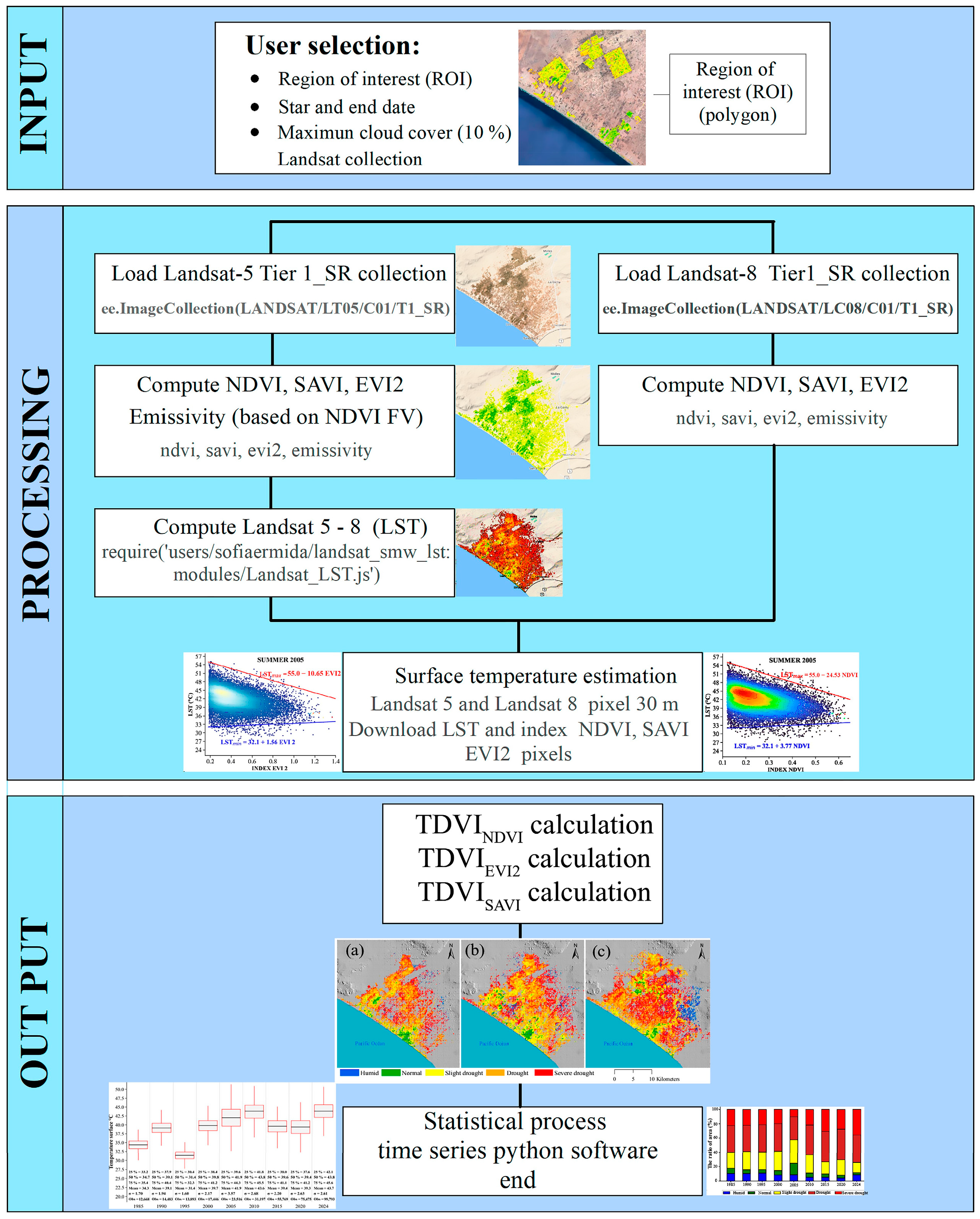
2. Materials and Methods
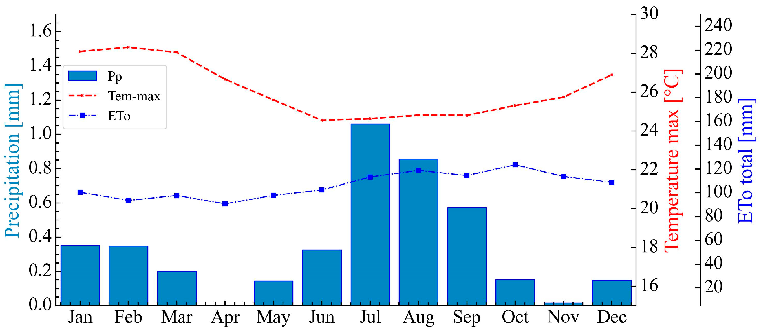
2.1. Study Area

The study area comprises the entire irrigation of the Caplina aquifer (Figure 1), located in the province and region of Tacna in southern Peru at the head of the Atacama Desert. It has a temperate-warm, desert climate with mean annual maximum and minimum temperatures (1950–2024 period) of 23.6 °C and 12.7 °C (Figure 2). Annual rainfall is scarce and even non-existent, characteristic of the driest desert in the world [8,31,32,33]; the water deficit does not allow agricultural demands to be met, so groundwater is used almost entirely. Moreover, the predominant crop is the olive tree, which faces extreme stress conditions, with planting frames of 5 × 5, 7 × 7 and 10 × 10 m, mostly under drip irrigation [7].

2.2. Landsat Satellite Data Acquisition and Image Preprocessing

The processing of Landsat 5 and 8 satellite images was carried out using the Google Earth Engine (GEE) platform, following certain specifications, such as selecting images with a percentage of cloud cover lower than 10% during the summer months (December, January, February and March) (Table 1). Vegetation indices (NDVI, SAVI and EVI2) and emissivity (based on NDVI-fv) were generated to obtain the LST as indicated by [28]. To define the region of interest (ROI) of the olive plots in the Caplina aquifer, NDVI was used, as detailed in Section 2.3, which allowed the generation of mask layers for the study years (1985–2024). Then, the triangulation method was applied between the LST and the vegetation indices, which allowed for the establishment of thresholds for wet and dry conditions (Section 2.5). Finally, obtaining these thresholds enabled an analysis of vegetation cover and the classification of the TVDI-VIs (Figure 3).

2.3. The Region of Interest (ROI) as a Function of Olive Crop Vigour Status

NDVI is an important indicator of crop vigour, so it was used to determine the regions of interest (ROI) according to the vigour characteristic of the olive tree. Research by [7] identified olive crop vigour ranges for arid areas as 0.1 to 0.21 (withered), 0.21 to 0.25 (severe), 0.25 to 0.37 (moderate), 0.37 to 0.42 (light) and 0.42 to 1.0 (healthy).

2.4. Vegetation Indices with Red (R) and Near-Infrared (NIR) Bands

The NIR and R spectral bands show the best performance of crop conditions. NDVI [19], defined by the wavelength of the R-band (0.630 to 0.680 µm) and the NIR (0.845 to 0.885 µm), which represents the photosynthetic activity of the leaf structure, is widely used (Equation (1)). EVI2 [20], like NDVI, is a unitless continuous variable and ranges from −1 to 1 (Equation (2)). However, they have limitations related to the brightness of the soil background. In contrast, SAVI [21] is considerably less susceptible to background variations caused by soil colouration or moisture present on the soil surface compared to other vegetation indices (Equation (3)).
N D V I = ( N I R R ) / ( N I R + R )
E V I 2 = 2.5 × ( N I R R ) / ( N I R + 2.4 × R + 1 )
S A V I = N I R R / ( N I R + R + L ) × ( 1 + L )
where NIR and R are the reflectances in the near-infrared (NIR) and red bands. L is the soil adjustment factor with a value of 0.5.

2.5. Land Surface Temperature from Landsat 5 and 8

LST estimates from high-resolution Landsat satellite imagery generated by [28] are available in the GEE public repository at the following link: (https://code.earthengine.google.com/?accept_repo=users/sofiaermida/landsat_smw_lst, accessed on 22 September 2023). This repository contains the Statistical Mono-Window (SMW) algorithm developed by the Climate Monitoring Satellite Application Facility (CM-SAF). In addition to the algorithms available in the GEE catalogue, atmospheric data from the National Center for Environmental Prediction (NCEP) and National Center for Atmospheric Research (NCAR) reanalyses, and emissivity data from the Advanced Spaceborne Thermal Emission and Reflection Radiometer Global Emissivity Database (ASTER GEDv3) set developed by the National Aeronautics and Space Administration (NASA, Washington, DC, USA) were used. These data were corrected using NDVI to account for vegetation dynamics. In addition to being validated by 12 in situ stations distributed across the United States and European countries, they indicate an overall accuracy of 0.5 K, −0.1 K and 0.2 K and an overall RMSE of 2.0 K, 2.1 K and 2.1 K for Landsat 5, 7 and 8.

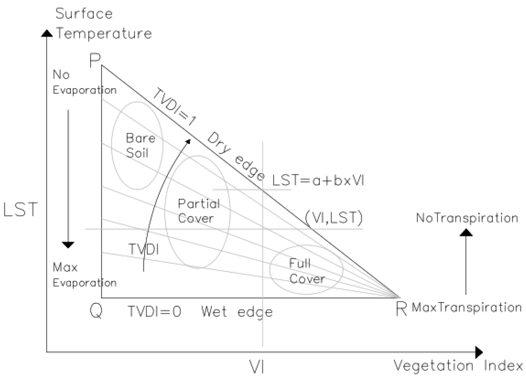
2.6. Temperature Vegetation Dryness Index (TVDI)

LST, which is sensitive to surface soil moisture in bare soil or sparsely vegetated conditions, varies depending on the vegetation (chlorophyll), which is reflected in the VIs. The scatter diagrams of LST and VIs are usually triangular [15] or trapezoidal [34] in shape (Figure 4). In the case of the triangle, the lower edge represents the maximum evaporation from the soil, while the upper edge indicates no evaporation at all. The negative slope at the dry edge reflects how the maximum LST decreases with increasing VIs. As NDVI increases, maximum LST decreases and TVDI increases from zero to one, signalling a change from extreme wet to extreme dry conditions. Equation (4) is as follows:
T V D I = ( L S T L S T m i n ) / ( L S T m a x L S T m i n )
where LST represents the land surface temperature, and LSTmin and LSTmax are the minimum and maximum land surface temperatures of pixels with the same VI in a specified region. These temperatures are used as a reference to define the “wet” and “dry” limits. LSTmin and LSTmax are calculated from groups of points located at the lower and upper ends of the scatter diagrams, and their Equations are (5) and (6).
L S T m i n = ( a 1 + b 1 × V I )
L S T m a x = ( a 2 + b 2 × V I )
where a1, b1, a2 and b2 are the linear fit coefficients of the wet edge and dry edge function.

3. Results

3.1. Estimation of the Region of Interest (ROI) as a Function of Olive Crop Vigour Status

Figure 5 shows the bar charts classifying the important characteristics of olive crop vigour (wilted, severe, moderate, mild and healthy), showing the area of interest in hectares, respectively. From 1985 to 2000, no significant changes are observed, with an average of 5633.75 ha. From 2005 (9427.2 ha) to 2024 (35,559.7 ha), a significant progressive increase is seen (Table 2). Furthermore, the characteristic with the highest average area from 1985 to 2024 is wilting with 48%, followed by moderate with 27%, severe with 14%, and finally mild and healthy with 5% and 6%, respectively.

3.2. Temporal Land Surface Temperature Variability

Figure 6 shows the LST (°C) of the agricultural area classified according to olive vigour in the reference period (1985–2024). The variability in the boxplots represents the summer season, with means and standard deviations in the warm years of 2005 (41.9 ± 3.57), 2010 (43.6 ± 2.68) and 2024 (43.7 ± 2.61); the year with the lowest temperature was 1995 (31.4 ± 1.60).

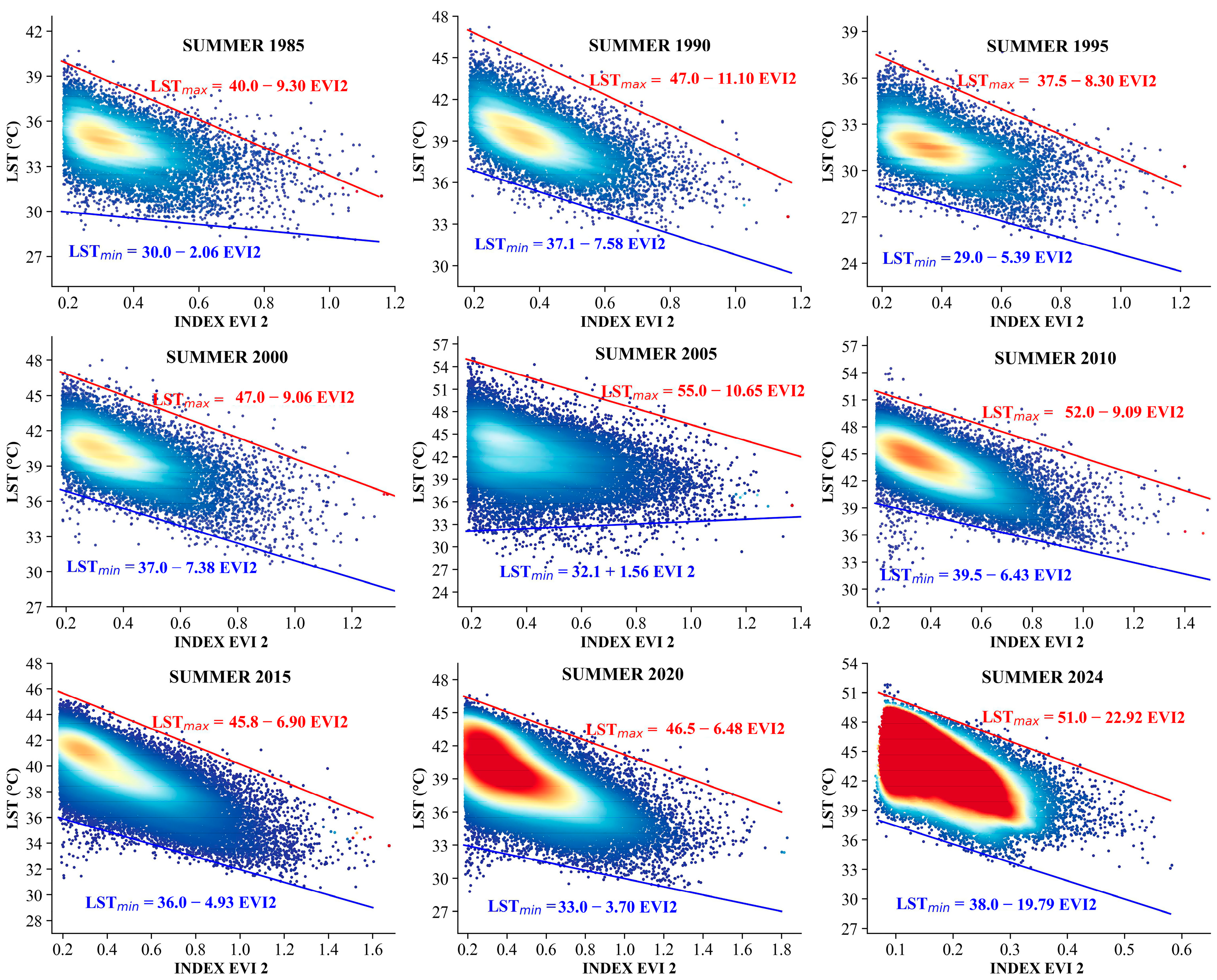
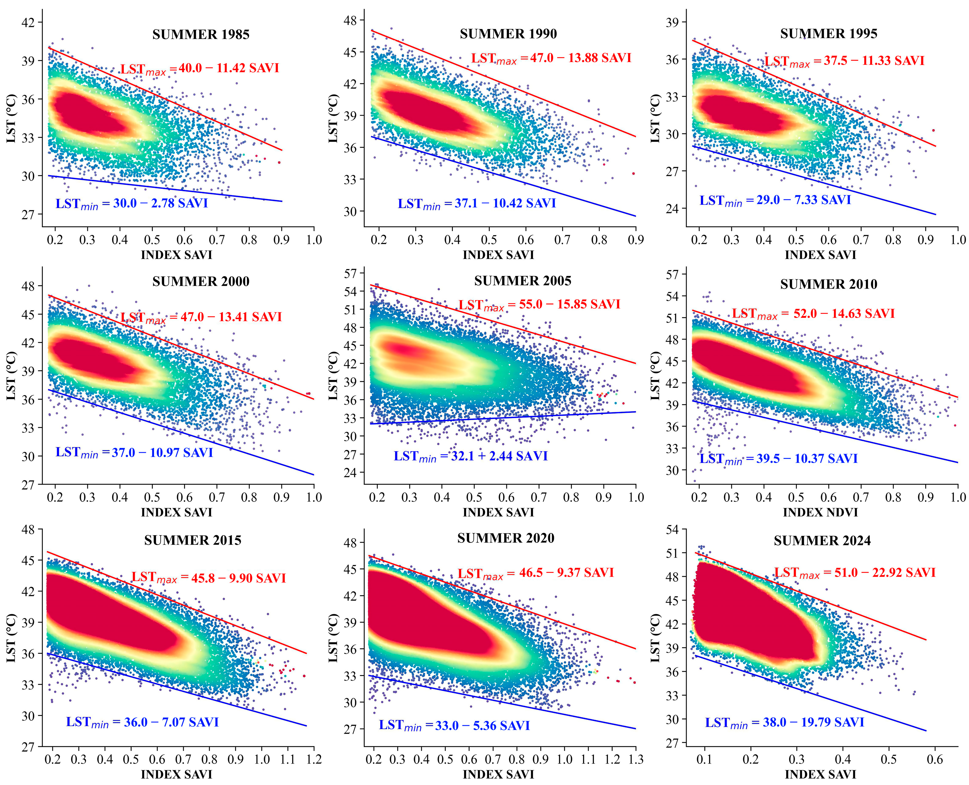
3.3. Calculation of LST-NDVI, EVI2 and SAVI Trapezoidal Thermo Space

The concentration of pixels in the thermal trapezoidal space of LST (NDVI, EVI2 and SAVI) is shown in Figure 7, Figure 8 and Figure 9, preserving the values of the constants a1 (wet edge) and a2 (dry edge) for the three cases of LST (NDVI, EVI2 and SAVI). A negative slope is observed in all plots except 2005, which has a positive slope at the dry edge. However, the constants b1 and b2 referred to in the VIs are different for each case. In addition, a higher presence of the concentration of bare soil, partial cover and full cover pixels is observed in all three cases in the years 2020 and 2024, except in the LST-SAVI, which shows this for the years 2010, 2015, 2020 and 2024.

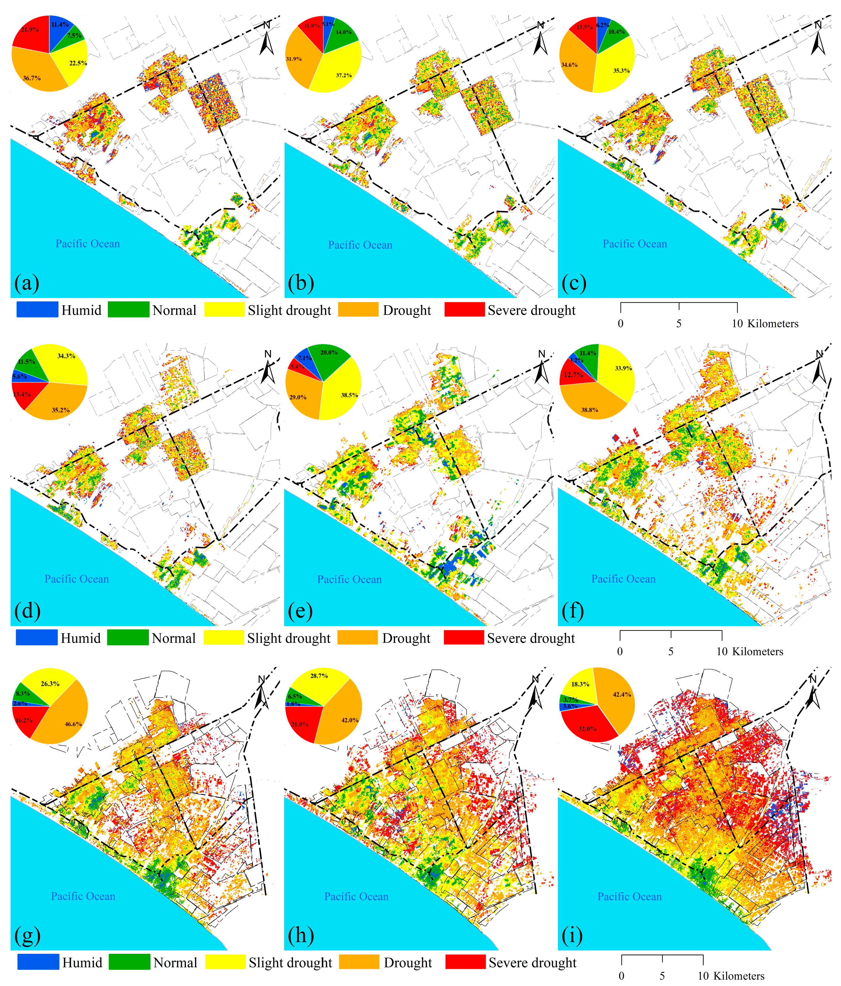
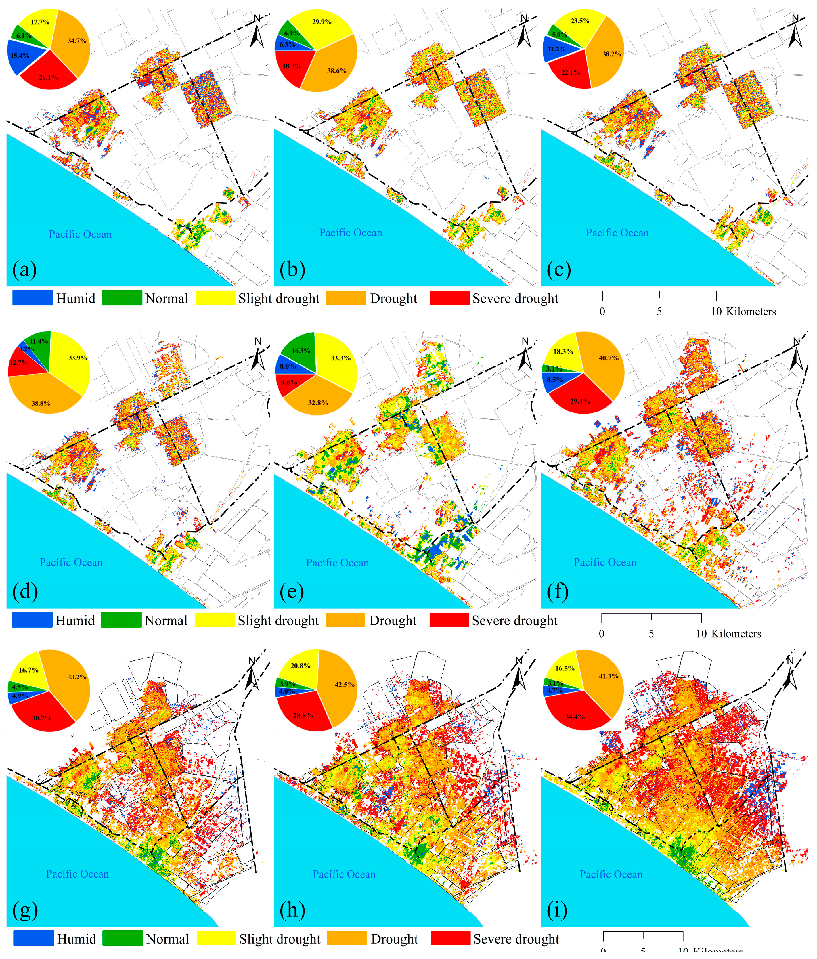
3.4. Spatio-Temporal Evolution of the TVDI with Respect to VI in the Caplina Aquifer

The spatio-temporal evolution of TVDINDVI, TVDIEVI2 and TVDISAVI, according to drought classification, is shown (Figure 10, Figure 11 and Figure 12). In addition, the increase of agricultural olive fields from 1985 to 2024 is observed. The TVDINDVI in 2024 presents higher percentages in drought with 37% (13,102.4 ha), which represents a significant increase compared to previous years. In contrast, severe drought presented a percentage higher than 40% in the years 2010, 2015 and 2020, while in 2024 it obtained 38% (13,552.1 ha). However, slight drought decreased from 33% (3071.0 ha) to 15% (5211.0 ha) from 2005 to 2024. Similarly, the classification for normal decreased from 2005 onwards, with 16% (1501.4 ha) in 2005 and 3% (1118.7 ha) by 2024. Finally, humid classification remained between 4 and 8% (Table 3).
The TVDIEVI2 (Figure 11) presented as severe drought for 2024 with a percentage higher than previous years of 32% (11,362.9 ha); for drought, on the other hand, it showed 42% (15,093.9 ha). However, slight drought and normal showed 18% (6512 ha) and 4% (1304.5 ha), respectively, showing a decrease compared to previous years. Finally, humid classification presented as 4% (1285.8 ha), higher by 1 and 2% compared to 2010, 2015 and 2020 (Table 4).
Figure 12 of the TVDISAVI shows the ranking for 2024 with the highest percentage of 34.4% (12,234.2 ha) for severe drought compared to previous years. However, for drought, it was 41% (14,692.4 ha), lower by 2% than 2015 and 2020. In addition, slight drought, normal and humid classifications, with 16% (5854.8 ha), 3% (1106.7 ha) and 5% (1671.6 ha), respectively, have slightly lower percentages than previous years (Table 5).

4. Discussion

4.1. Analysis of NDVI Classification for Olive Tree Vigour

NDVI is an excellent indicator of vigour and water stress in the crop. Its vigour classification was carried out in a previous study by [7], in plantations from 3 to 60 years old, using different VIs (NDVI, DVI, SAVI, GNDVI, EVI2 and MSAVI), obtained through spectral ranges that classify vigour as wilted, severe, moderate, mild and healthy. This study was considered highly relevant because it was conducted in an area within our study area. However, NDVI classification can be influenced by cover and soil type, similar to LST for detecting water stress. On the other hand, the study by [10] recommends the use of thermal sensors for the detection of water stress in olive trees. As for the NDVI vigour classification in the Caplina aquifer, it presented a problem with more than 50% (withered) of the total olive tree area (Table 2). This may be due to the fact that the NDVI values were extracted in the summer months, in addition to being a semi-arid area with a high presence of salinity in the soils.

4.2. Analysis of the LST-VIs Feature Space

The characteristics of the LST-VI data in the study area and the determination of the dry and wet edge with respect to NDVI, EVI2 and SAVI are presented in Figure 7, Figure 8 and Figure 9. The VIs, specifically made up of infrared bands (red and near infrared), have a higher representation of the canopy cover [4,35]. It can be concluded that the pixel concentration spaces form a trapezoid due to the negative slopes of the VIs, except for the year 2005, for which they present a positive slope at the wet edge, whose trend would represent a triangle. According to [34], the relationship of LST-VIs can be triangular or trapezoidal. Likewise, [9,35] state that if the slope is positive at the wet edge, it reflects that the minimum LST increases as the VIs decrease.

4.3. Analysis of Spatial and Temporal Variation Trend in TVDI

TVDI was mainly affected by increased land use and climatic factors. The results of TVDINDVI, TVDISAVI and TVDIEVI2 show significant differences in each year, but do show a difference in the classification trend in the period from 1985 to 2024. The mean and standard deviation of the percentage of area were obtained for severe drought (24 ± 7.4%), drought (39 ± 3.2%), mild drought (23 ± 5.25%), normal (7 ± 3.7%) and wet (7 ± 2.5%) for TVDINDVI. Similar percentages were obtained for TVDISAVI, except for TVDIEVI2, which showed severe drought (16 ± 7.64%), drought (37 ± 5.5%), mild drought (23 ± 5.2%), normal (10 ± 4.7%) and wet (5 ± 2.9%). It is stated that TVDINDVI and TVDISAVI are very similar. According to [12], it mentions that TVDISAVI and TVDINDVI are better indicators specifically in semi-arid areas, where high salinity is found in soils. In addition, it was not possible to compare with SPI or to apply another hydrological method due to minimal rainfall (Figure 2), being in a semi-arid area. However, from 2005 onwards there was an excessive increase in land use for agriculture [31,32], increasing cultivated areas and water needs, leading to the need to drill new wells and causing overexploitation and marine intrusion problems in the Caplina aquifer [32,33]. In areas with drought, which were predominant in all years of the study, there was also a tendency to severe drought. These conditions are due to being a semi-arid zone with minimal or no rainfall, in addition to the overexploitation of aquifers [33]. In sandy areas, it is necessary to optimise the irrigation system with highly efficient and water-saving agricultural methods [12,15]. Drought affects the state of vegetation, the water cycle and human life [23].

Climatological and Phenological Factor

The range of the study months represents the summer season, the months with the highest temperatures during which the water requirement is critical. Also, because of the irrigation interval, most of the fields from 1995 to 2005 were irrigated by gravity irrigation [7]. However, from 2005 to 2024 the use of drip irrigation will have increased exponentially [32]. The study years show the same trend of drought, except in 2005 when there was a decrease in severe drought and drought, obtaining a higher percentage in moderate drought (Table 3, Table 4 and Table 5). This is attributed to the presence of the El Niño-Southern Oscillation (ENSO) phenomenon, which manifested itself in the Central Pacific (CP) in 2005, resulting in the absence of drought on the southern coast of Peru [36,37,38]. Studies on drought prediction, globally and in Peru, tend to focus more on the Peruvian coastal regions [38]. On the other hand, olive cultivation is in the fruiting phenological stage, a period in which its water needs are critical, requiring constant irrigation to achieve better yield and fruit quality [5,10,11].

4.4. Limitations and Future Research

In this study, we verified the capability of TVDI with respect to three different VIs in drought monitoring in the main crop of southern Peru and obtained good results. However, TVDI still presents some uncertainties. Therefore, TVDI needs to be validated with moisture sensors and stomatal conductance measurements to assess the effects of water stress on stomatal closure and thermal energy dissipation pathways. The advancement of remote sensing technology with thermal and hyperspectral sensors coupled to unmanned aerial vehicles (UAVs) with high spectral resolution has advantages in orchard or plot level monitoring and drought application that traditional remote sensing does not possess. Imagery can be obtained at any time necessary for crop monitoring [15,18]. In future research, a modified TVDI should be developed that integrates a triangular feature space with temperature data from the thermal sensor and hyperspectral imagery captured by UAVs.

5. Conclusions

In this study, a freely available remote sensing tool, the GEE platform, was used to obtain LST and VIs (NDVI, EVI2 and SAVI) from Landsat 5 and 8 and estimate the water status of olive cultivation in arid areas, specifically during the summer season from 1985 to 2024. Consequently, TVDI can be an effective parameter to detect changes in land use and water stress. Both TVDI and VI showed variations in vegetation density and surface temperature between 2005 and 2024. However, TVDINDVI and TVDISAVI are more sensitive for detecting water stress than TVDIEVI2, especially in the interaction of trapezoidal pixels. On the other hand, the presence of TVDI anomalies in 2005 is consistent with ENSO, with a greater presence of moderate drought zones compared to later years (2010, 2015, 2020 and 2024), which showed a greater increase in the drought zone. It is suggested for future research to obtain information from infrared sensors that allow for a more precise identification of water stress in different seasons of the year, as well as the use of UAVs. This study will be reflected in water stress maps of olive cultivation in the Caplina aquifer to provide options to address current and future problems in the management of water resources in the olive sector in the semi-arid areas of southern Peru.

Author Contributions

Conceptualization, J.A.Q.-M., E.P.-V., G.H. and L.R.-F.; methodology, J.A.Q.-M., E.P.-V., S.C.-M. and G.H.; software, J.A.Q.-M. and G.H.; validation, E.P.-V., L.R.-F., B.V.-B., J.E.-M. and F.C.-O.; formal analysis, J.A.Q.-M., G.H., E.P.-V., S.C.-M., B.V.-B., J.E.-M., L.R.-F and F.C.-O.; investigation, J.A.Q.-M., G.H., E.P.-V., S.C.-M., B.V.-B., L.R.-F and F.C.-O.; resources, E.P.-V.; data curation, E.P.-V.; writing—original draft preparation, J.A.Q.-M., E.P.-V. and G.H.; writing—review and editing, E.P.-V., S.C.-M., B.V.-B., L.R.-F, J.E.-M. and F.C.-O.; supervision, E.P.-V.; project administration, E.P.-V.; funding acquisition, E.P.-V. and F.C.-O. All authors have read and agreed to the published version of the manuscript.

Funding

This research is funded by canon, over canon and mining royalties from the Jorge Basadre Grohmann National University, Vice-rector for Research, project “Use of remote sensors to improve irrigation management in olive trees (Olea europaea L.), and confront climate change in arid zones”. Rectoral Resolution No. 11174-2023-UNJBG.

Institutional Review Board Statement

Not applicable.

Data Availability Statement

Data are contained within the article.

Conflicts of Interest

The authors declare no conflicts of interest.

References

  1. Adeyeri, O.E.; Folorunsho, A.H.; Ayegbusi, K.I.; Bobde, V.; Adeliyi, T.E.; Ndehedehe, C.E.; Akinsanola, A.A. Land Surface Dynamics and Meteorological Forcings Modulate Land Surface Temperature Characteristics. Sustain. Cities Soc. 2024, 101, 105072. [Google Scholar] [CrossRef]
  2. Dimyati, M.; Aginta, F.; Damayanti, A. The Effect of Vegetation Index on the Land Surface Temperature in South Badung Regency, Bali Province the Effect of Vegetation Index on the Land Surface Temperature in South Badung Regency, Bali Province. IOP Conf. Ser. Earth Environ. Sci. 2024, 1291, 012024. [Google Scholar] [CrossRef]
  3. Przeździecki, K.; Zawadzki, J. Assessing Moisture Content and Its Mitigating Effect in an Urban Area Using the Land Surface Temperature–Vegetation Index Triangle Method. Forests 2023, 14, 578. [Google Scholar] [CrossRef]
  4. Mohanasundaram, S.; Baghel, T.; Thakur, V.; Udmale, P.; Shrestha, S. Reconstructing NDVI and Land Surface Temperature for Cloud Cover Pixels of Landsat-8 Images for Assessing Vegetation Health Index in the Northeast Region of Thailand; Springer International Publishing: Berlin/Heidelberg, Germany, 2023; Volume 195, ISBN 0123456789. [Google Scholar]
  5. Torres, M.; Pierantozzi, P.; Searles, P.; Cecilia Rousseaux, M.; García-Inza, G.; Miserere, A.; Bodoira, R.; Contreras, C.; Maestri, D. Olive Cultivation in the Southern Hemisphere: Flowering, Water Requirements and Oil Quality Responses to New Crop Environments. Front. Plant Sci. 2017, 8, 294457. [Google Scholar] [CrossRef] [PubMed]
  6. Gómez-del-Campo, M.; Pérez-Expósito, M.Á.; Hammami, S.B.M.; Centeno, A.; Rapoport, H.F. Effect of Varied Summer Deficit Irrigation on Components of Olive Fruit Growth and Development. Agric. Water Manag. 2014, 137, 84–91. [Google Scholar] [CrossRef]
  7. Pino-Vargas, E.; Huayna, G. Spatial and Temporal Evolution of Olive Cultivation Due to Pest Attack, Using Remote Sensing and Satellite Image Processing. Sci. Agropecu. 2022, 13, 149–157. [Google Scholar] [CrossRef]
  8. Machaca-Pillaca, R.; Pino-Vargas, E.; Ramos-Férnandez, L.; Quille-Mamani, J.; Torres-Rua, A. Estimación de La Evapotranspiración Con Fines de Riego En Tiempo Real de Un Olivar a Partir de Imágenes de Un Drone En Zonas Áridas, Caso La Yarada, Tacna, Perú. Idesia 2022, 40, 55–65. [Google Scholar] [CrossRef]
  9. Zare, M.; Drastig, K.; Zude-Sasse, M. Tree Water Status in Apple Orchards Measured by Means of Land Surface Temperature and Vegetation Index (LST-NDVI) Trapezoidal Space Derived from Landsat 8 Satellite Images. Sustainability 2020, 12, 70. [Google Scholar] [CrossRef]
  10. Sepulcre-Cantó, G.; Zarco-Tejada, P.J.; Jiménez-Muñoz, J.C.; Sobrino, J.A.; De Miguel, E.; Villalobos, F.J. Detection of Water Stress in an Olive Orchard with Thermal Remote Sensing Imagery. Agric. For. Meteorol. 2006, 136, 31–44. [Google Scholar] [CrossRef]
  11. Kefi, M.; Pham, T.D.; Kashiwagi, K.; Yoshino, K. Identification of Irrigated Olive Growing Farms Using Remote Sensing Techniques. Euro-Mediterr. J. Environ. Integr. 2016, 1, 3. [Google Scholar] [CrossRef]
  12. Du, L.; Song, N.; Liu, K.; Hou, J.; Hu, Y.; Zhu, Y.; Wang, X.; Wang, L.; Guo, Y. Comparison of Two Simulation Methods of the Temperature Vegetation Dryness Index (TVDI) for Drought Monitoring in Semi-Arid Regions of China. Remote Sens. 2017, 9, 177. [Google Scholar] [CrossRef]
  13. Babaeian, E.; Sadeghi, M.; Franz, T.E.; Jones, S.; Tuller, M. Mapping Soil Moisture with the OPtical TRApezoid Model (OPTRAM) Based on Long-Term MODIS Observations. Remote Sens. Environ. 2018, 211, 425–440. [Google Scholar] [CrossRef]
  14. Amani, M.; Salehi, B.; Mahdavi, S.; Masjedi, A.; Dehnavi, S. Temperature-Vegetation-Soil Moisture Dryness Index (TVMDI). Remote Sens. Environ. 2017, 197, 1–14. [Google Scholar] [CrossRef]
  15. Liu, Y.; Ni, Z.; Zhao, Y.; Zhou, G.; Luo, Y.; Li, S.; Wang, D.; Zhang, S. Spatial-Temporal Evolution and Driving Forces of Drying Trends on the Qinghai-Tibet Plateau Based on Geomorphological Division. Int. J. Environ. Res. Public Health 2022, 19, 7909. [Google Scholar] [CrossRef] [PubMed]
  16. Tirivarombo, S.; Osupile, D.; Eliasson, P. Drought Monitoring and Analysis: Standardised Precipitation Evapotranspiration Index (SPEI) and Standardised Precipitation Index (SPI). Phys. Chem. Earth 2018, 106, 1–10. [Google Scholar] [CrossRef]
  17. Beguería, S.; Vicente-Serrano, S.M.; Angulo-Martínez, M. A Multiscalar Global Drought Dataset: The SPEI Base: A New Gridded Product for the Analysis of Drought Variability and Impacts. Bull. Am. Meteorol. Soc. 2010, 91, 1351–1356. [Google Scholar] [CrossRef]
  18. Dai, R.; Chen, S.; Cao, Y.; Zhang, Y.; Xu, X. A Modified Temperature Vegetation Dryness Index (MTVDI) for Agricultural Drought Assessment Based on MODIS Data: A Case Study in Northeast China. Remote Sens. 2023, 15, 1915. [Google Scholar] [CrossRef]
  19. Huang, S.; Tang, L.; Hupy, J.P.; Wang, Y.; Shao, G. A Commentary Review on the Use of Normalized Difference Vegetation Index (NDVI) in the Era of Popular Remote Sensing. J. For. Res. 2021, 32, 1–6. [Google Scholar] [CrossRef]
  20. Mondal, P. Quantifying Surface Gradients with a 2-Band Enhanced Vegetation Index (EVI2). Ecol. Indic. 2011, 11, 918–924. [Google Scholar] [CrossRef]
  21. Huete, A.R. A Soil-Adjusted Vegetation Index (SAVI). Remote Sens. Environ. 1988, 25, 295–309. [Google Scholar] [CrossRef]
  22. Guha, S.; Govil, H. An Assessment on the Relationship between Land Surface Temperature and Normalized Difference Vegetation Index. Environ. Dev. Sustain. 2021, 23, 1944–1963. [Google Scholar] [CrossRef]
  23. Chen, J.; Wang, C.; Jiang, H.; Mao, L.; Yu, Z. Estimating Soil Moisture Using Temperature-Vegetation Dryness Index (TVDI) in the Huang-Huai-Hai (HHH) Plain. Int. J. Remote Sens. 2011, 32, 1165–1177. [Google Scholar] [CrossRef]
  24. Zhen, Z.; Chen, S.; Yin, T.; Gastellu-Etchegorry, J.P. Globally Quantitative Analysis of the Impact of Atmosphere and Spectral Response Function on 2-Band Enhanced Vegetation Index (EVI2) over Sentinel-2 and Landsat-8. ISPRS J. Photogramm. Remote Sens. 2023, 205, 206–226. [Google Scholar] [CrossRef]
  25. Rahimzadeh-Bajgiran, P.; Omasa, K.; Shimizu, Y. Comparative Evaluation of the Vegetation Dryness Index (VDI), the Temperature Vegetation Dryness Index (TVDI) and the Improved TVDI (ITVDI) for Water Stress Detection in Semi-Arid Regions of Iran. ISPRS J. Photogramm. Remote Sens. 2012, 68, 1–12. [Google Scholar] [CrossRef]
  26. Singh, P.; Verma, P.; Chaudhuri, A.S.; Singh, V.K.; Rai, P.K. Evaluating the Relationship between Urban Heat Island and Temporal Change in Land Use, NDVI and NDBI: A Case Study of Bhopal City, India. Int. J. Environ. Sci. Technol. 2023, 21, 3061–3072. [Google Scholar] [CrossRef]
  27. Değermenci, A.S. Estimation of Land Surface Temperature from Landsat-8 OLI: Comparative Analysis of Two Periods for Duzce in Turkey. Int. J. Environ. Sci. Technol. 2024, 21, 6389–6404. [Google Scholar] [CrossRef]
  28. Ermida, S.L.; Soares, P.; Mantas, V.; Göttsche, F.M.; Trigo, I.F. Google Earth Engine Open-Source Code for Land Surface Temperature Estimation from the Landsat Series. Remote Sens. 2020, 12, 1471. [Google Scholar] [CrossRef]
  29. Quintana-Molina, J.R.; Sánchez-Cohen, I.; Jiménez-Jiménez, S.I.; de Marcial-Pablo, M.J.; Trejo-Calzada, R.; Quintana-Molina, E. Calibration of Volumetric Soil Moisture Using Landsat-8 and Sentinel-2 Satellite Imagery by Google Earth Engine. Rev. Teledetec. 2023, 2023, 21–38. [Google Scholar] [CrossRef]
  30. Olmos-Trujillo, E.; González-Trinidad, J.; Júnez-Ferreira, H.; Pacheco-Guerrero, A.; Bautista-Capetillo, C.; Avila-Sandoval, C.; Galván-Tejada, E. Spatio-Temporal Response of Vegetation Indices to Rainfall and Temperature in a Semiarid Region. Sustainability 2020, 12, 1939. [Google Scholar] [CrossRef]
  31. Edwin Pino, V.; Eduardo Chávarri, V. Evidence of Climate Change in the Hyper-Arid Region of the Southern Coast of Peru, Head of the Atacama Desert. Tecnol. Ciencias Agua 2022, 13, 333–375. [Google Scholar] [CrossRef]
  32. Pino-Vargas, E.; Espinoza-Molina, J.; Chávarri-Velarde, E.; Quille-Mamani, J.; Ingol-Blanco, E. Impacts of Groundwater Management Policies in the Caplina Aquifer, Atacama Desert. Water 2023, 15, 2610. [Google Scholar] [CrossRef]
  33. Pino, E.; Ramos, L.; Avalos, O.; Tacora, P.; Chávarri, E.; Angulo, O.; Ascensios, D.; Mejía, J. Factors Affecting Depletion and Pollution by Marine Intrusion in the La Yarada’s Coastal Aquifer, Tacna, Peru. Tecnol. Ciencias Agua 2019, 10, 177–213. [Google Scholar] [CrossRef]
  34. Pandey, R.; Goswami, S.; Sarup, J.; Matin, S. The Thermal–Optical Trapezoid Model-Based Soil Moisture Estimation Using Landsat-8 Data. Model. Earth Syst. Environ. 2021, 7, 1029–1037. [Google Scholar] [CrossRef]
  35. Guha, S.; Govil, H. Land Surface Temperature and Normalized Difference Vegetation Index Relationship: A Seasonal Study on a Tropical City. SN Appl. Sci. 2020, 2, 1661. [Google Scholar] [CrossRef]
  36. Imfeld, N.; Barreto Schuler, C.; Correa Marrou, K.M.; Jacques-Coper, M.; Sedlmeier, K.; Gubler, S.; Huerta, A.; Brönnimann, S. Summertime Precipitation Deficits in the Southern Peruvian Highlands since 1964. Int. J. Climatol. 2019, 39, 4497–4513. [Google Scholar] [CrossRef]
  37. Mortensen, E.; Wu, S.; Notaro, M.; Vavrus, S.; Montgomery, R.; De Piérola, J.; Sánchez, C.; Block, P. Regression-Based Season-Ahead Drought Prediction for Southern Peru Conditioned on Large-Scale Climate Variables. Hydrol. Earth Syst. Sci. 2018, 22, 287–303. [Google Scholar] [CrossRef]
  38. Potter, E.R.; Fyffe, C.L.; Orr, A.; Quincey, D.J.; Ross, A.N.; Rangecroft, S.; Medina, K.; Burns, H.; Llacza, A.; Jacome, G.; et al. A Future of Extreme Precipitation and Droughts in the Peruvian Andes. NPJ Clim. Atmos. Sci. 2023, 6, 96. [Google Scholar] [CrossRef]
Figure 1. (a) Digital elevation model of southern Peru with the red square showing the study area. (b) Location map of the Caplina aquifer, located in the southern region of Peru. (c) Landsat 8 visible image (red, green and blue) of the agricultural irrigation zone of the Caplina aquifer in 2024. Subfigures (ac), show the purple and white lines marking the border with Chile.
Agriculture 14 00662 g001
Figure 2. Changes in annual precipitation, average annual temperature and average annual potential evapotranspiration from 1985 to 2024.
Agriculture 14 00662 g002
Figure 3. Working diagram of the processing of Landsat 5 and 8 satellite images in the Google Earth Engine platform for the period 1985–2024. Subfigures (ac), show the Temperature Vegetation Dryness Indices TVDINDVI, TVDISAVI and TVDIEVI2 for 2024.
Agriculture 14 00662 g003
Figure 4. The LST–VI triangle space and the definition of the TVDI (adapted from [18]).
Agriculture 14 00662 g004
Figure 5. Temporal variation in cumulative areas (1985 to 2024) of normalised vegetation index (NDVI) classes of olive crop vigour status.
Agriculture 14 00662 g005
Figure 6. Land surface temperature (LST) variability in summer season boxplots from 1985 to 2024.
Agriculture 14 00662 g006
Figure 7. Pixel distributions for the combination of shallow irrigated and rainfed agricultural areas within LST-NDVI; the red line represents the dry edge and the blue line the wet edge.
Agriculture 14 00662 g007
Figure 8. Pixel distributions for the combination of shallow irrigated and rainfed agricultural areas within LST-EVI2; the red line represents the dry edge and the blue line the wet edge.
Agriculture 14 00662 g008
Figure 9. Pixel distributions for the combination of shallow irrigated and rainfed agricultural areas within LST-SAVI; the red line represents the dry edge and the blue line the wet edge.
Agriculture 14 00662 g009
Figure 10. Spatial and temporal variation in thematic maps of the water stress index ( T V D I N D V I ) (ai), in the period 1985 to 2020 every 5 years, and in 2024.
Agriculture 14 00662 g010
Figure 11. Spatial and temporal variation in thematic maps of the water stress index ( T V D I E V I 2 ) (ai), in the period 1985 to 2020 every 5 years, and in 2024.
Agriculture 14 00662 g011
Figure 12. Spatial and temporal variation in thematic maps of the water stress index ( T V D I S A V I ) (ai), in the period 1985 to 2020 every 5 years, and in 2024.
Agriculture 14 00662 g012
Table 1. Downloaded scenes, Landsat Collections, (https://developers.google.com/earth-engine/datasets/catalog/landsat accessed on 20 September 2023) and time period.
DataYearProduct IdentifierSensing Time (hh:mm:ss)Cloud Cover %Patch/Row
Landsat 51985LANDSAT/LT05/C01/T1_SR/LT05_002072_1985032814:12:01302/72
1985LANDSAT/LT05/C01/T1_SR/LT05_002073_1985032814:12:25802/73
Landsat 51990LANDSAT/LT05/C01/T1_SR/LT05_002072_1989120414:05:25202/72
1990LANDSAT/LT05/C01/T1_SR/LT05_002073_1990012114:04:21502/73
Landsat 51995LANDSAT/LT05/C01/T1_SR/LT05_002073_1995032413:51:52102/73
Landsat 52000LANDSAT/LT05/C01/T1_SR/LT05_002073_2000032114:16:05102/73
Landsat 52005LANDSAT/LT05/C01/T1_SR/LT05_002072_2005031914:28:38202/72
2005LANDSAT/LT05/C01/T1_SR/LT05_002073_2005031914:29:02002/73
Landsat 52010LANDSAT/LT05/C01/T1_SR/LT05_002073_2010021314:32:56902/73
Landsat 82015LANDSAT/LC08/C01/T1_SR/LC08_002073_2015031514:41:380.5502/73
Landsat 82020LANDSAT/LC08/C01/T1_SR/LC08_002072_2020032814:41:225.9802/72
2020LANDSAT/LC08/C01/T1_SR/LC08_002073_2020022514:42:016.4302/73
Landsat 82024LANDSAT/LC08/C02/T1_TOA/LC08_002073_2024020414:42:080.0502/73
Table 2. Normalised difference vegetation index (NDVI) classification area for each category of olive crop vigour stage.
VegetationDensityNDVI198519901995200020052010201520202024
ha%ha%ha%ha%ha%ha%ha%ha%ha%
Withered0.1–0.212644.1542389.8432431.4463212.1484278.0455743.44610,798.74913,859.74718,231.451
Severe0.21–0.25770.816966.918854.4161011.0151389.6151771.0142417.7113394.3124638.413
Moderate0.25–0.371196.4241761.0321555.6291867.2282659.1283459.9285410.6246841.2238776.625
Slight0.37–0.42167.93238.94256.65305.45486.35694.761450.371841.161968.56
Healthy0.42–1156.43159.73227.84361.75614.27702.262127.9103659.8121944.85
Total4935.51005516.31005325.81006757.41009427.210012,371.210022,205.210029,596.210035,559.7100
Table 3. Area by category of the water stress index TVDINDVI.
Vegetation DensityTVDINDVI198519901995200020052010201520202024
ha%ha%ha%ha%ha%ha%ha%ha%ha%
Humid0–0.2498.210558.710553.910535.48781.18596.051081.951112.942575.57
Normal0.2–0.4364.87308.16283.55448.571501.416737.761000.551207.941118.73
Slight drought0.4–0.61093.8221374.8251309.2251748.8263071.0333092.9253710.4176326.6215211.015
Drought0.6–0.81854.9382064.8372043.7382611.4393112.1335220.4429610.04312602.84313,552.138
Severe drought0.8–11123.8231210.0221135.3211413.321961.6102724.1226802.4318346.02813,102.437
Total4935.51005516.31005325.81006757.41009427.210012,371.210022,205.210029,596.210035,559.7100
Table 4. Area by category of the water stress index TVDIEVI2.
Vegetation DensityTVDIEVI2198519901995200020052010201520202024
ha%ha%ha%ha%ha%ha%ha%ha%ha%
Humid0–0.2562.111284.05332.66379.06670.87399.93579.93525.821285.84
Normal0.2–0.4371.78770.414555.010779.3121882.2201415.9111833.181913.071304.54
Slight drought0.4–0.61111.7232054.1371879.4352317.4343630.3394189.2345851.4268505.7296512.718
Drought0.6–0.81811.4371758.3321840.4352378.2352732.5294801.73910,352.84712,439.94215,093.942
Severe drought0.8–11078.722649.612718.514903.413511.551564.5133588.0166211.82111,362.932
Total4935.51005516.31005325.81006757.41009427.210012371.210022,205.210029,596.210035,559.7100
Table 5. Area by category of the water stress index TVDISAVI.
Vegetation DensityTVDISAVI198519901995200020052010201520202024
ha%ha%ha%ha%ha%ha%ha%ha%ha%
Humid0–0.2744.015349.86592.611758.011757.781045.491084.551188.641671.65
Normal0.2–0.4300.46382.57264.55286.243136.116385.33998.751159.541106.73
Slight drought0.4–0.6879.6181649.4301252.7241383.5211543.8332261.5183707.1176148.8215854.816
Drought0.6–0.81720.7352127.5392036.4382606.5393087.6335039.0419605.94312,569.24314,692.441
Severe drought0.8–11290.8261007.1181179.5221723.226902.1103640.0296808.9318530.02912,234.234
Total4935.51005516.31005325.81006757.41009427.210012,371.210022,205.210029,596.210035,559.7100
Disclaimer/Publisher’s Note: The statements, opinions and data contained in all publications are solely those of the individual author(s) and contributor(s) and not of MDPI and/or the editor(s). MDPI and/or the editor(s) disclaim responsibility for any injury to people or property resulting from any ideas, methods, instructions or products referred to in the content.

