3D Reconstruction of Wheat Plants by Integrating Point Cloud Data and Virtual Design Optimization

Abstract

The morphology and structure of wheat plants are intricate, containing numerous tillers, rich details, and significant cross-obscuration. Methods of effectively reconstructing three-dimensional (3D) models of wheat plants that reflects the varietal architectural differences using measured data is challenging in plant phenomics and functional–structural plant models. This paper proposes a 3D reconstruction technique for wheat plants that integrates point cloud data and virtual design optimization. The approach extracted single stem number, growth position, length, and inclination angle from the point cloud data of a wheat plant. It then built an initial 3D mesh model of the plant by integrating a wheat 3D phytomer template database with variety resolution. Diverse 3D wheat plant models were subsequently virtually designed by iteratively modifying the leaf azimuth, based on the initial model. Using the 3D point cloud of the plant as the overall constraint and setting the minimum Chamfer distance between the point cloud and the mesh model as the optimization objective, we obtained the optimal 3D model as the reconstruction result of the plant through continuous iterative calculation. The method was validated using 27 winter wheat plants, with nine varieties and three replicates each. The R² values between the measured data and the reconstructed plants were 0.80, 0.73, 0.90, and 0.69 for plant height, crown width, plant leaf area, and coverage, respectively. Additionally, the Normalized Root Mean Squared Errors (NRMSEs) were 0.10, 0.12, 0.08, and 0.17, respectively. The Mean Absolute Percentage Errors (MAPEs) used to investigate the vertical spatial distribution between the reconstructed 3D models and the point clouds of the plants ranged from 4.95% to 17.90%. These results demonstrate that the reconstructed 3D model exhibits satisfactory consistency with the measured data, including plant phenotype and vertical spatial distribution, and accurately reflects the characteristics of plant architecture and spatial distribution for the utilized wheat cultivars. This method provides technical support for research on wheat plant phenotyping and functional–structural analysis.

1. Introduction

Variety characteristics are reflected by the three-dimensional (3D) spatial morphology and structure of plants, as well as environmental and cultivation management practices. Traditional research methods assess the morphological features using leaf length, leaf area, canopy height, and leaf area index to characterize crop structure. However, it is challenging for these indices to depict the 3D spatial variances in plants. Additionally, they fail to meet the substantial requirement for high-resolution physiological and ecological mechanism analysis in crop science [1]. Consequently, it is crucial to investigate 3D plant modelling, which has evolved as a significant component of plant phenomics [2] and functional–structural plant modelling (FSPM) [3,4].

Three-dimensional plant model construction comprises two stages: 3D plant modelling [5] and 3D reconstruction [6]. Three-dimensional plant modelling is primarily employed to construct 3D plant models, using modelling software or customized 3D modelling techniques. The aim is to construct 3D models that reflect the topological characteristics of the varieties for visualization and computation, or to create 3D plant models with a realistic appearance for rendering and other applications using interactive methods. Typical software and methods include L-Studio [7], GroIMP [8], Helios [9], and XFrog. Plant modelling in 3D spans various scales, from cell to tissue, organ, individual, and population. Researchers have conducted multi-scale modelling around leaf growth, covering growth mechanisms at the cell scale to growth simulations at the leaf scale [10,11]. At the individual scale, growth models were integrated for the construction of a 4D model of maize plants [12]. Researchers have proposed constructing 3D models of maize populations by simulating their spatial distribution through statistical distribution models [13]. However, differences between 3D plant modeling methods and actual plants hinder their application in variety-centered crop science research.

Three-dimensional plant reconstruction [6,14] is necessary to obtain real-world data regarding the morphology and structure of plants through measured data, such as images or LiDAR. Computer graphics-related methods are then employed to construct a highly accurate and consistent 3D model of the target plant. Three-dimensional plant reconstruction holds significant value for crop science research, as it allows for the realistic reconstruction of plants on computers. This technology can be utilized to extract morphological and structural phenotypes of plants [15], as well as to analyze the light energy utilization efficiency of crops from various plant architectures [16]. However, the process of 3D plant reconstruction requires advanced technical methods. For instance, the creation of a 3D plant model utilizing 3D point cloud data entails a series of steps, including point cloud denoising, organ segmentation, feature extraction, mesh reconstruction, and mesh fusion [17].

Obtaining 3D point clouds of plants is the most commonly used technique for phenotype extraction and 3D reconstruction of plants, utilizing methods such as multi-view reconstruction, depth cameras [18], and LiDAR [19]. Point clouds are unstructured and cannot be used to directly extract phenotypic traits with semantic information, nor can they be directly used for visual calculation and analysis, such as light distribution estimation. However, the reconstructed mesh model is semantic, including phenotype traits, and can also be used for FSPM. It is worth noting that related studies tend to focus on plants with simple morphology and structures, such as maize and sorghum, or on specific organs such as plant leaves. For instance, one approach to achieving the 3D reconstruction of a maize plant involves slicing and clustering the leaf point cloud [20]. However, this method results in a flat leaf, losing the concave and convex leaf surface as well as the edge folding features. An alternate 3D reconstruction technique, which utilizes the Self-Organized Map algorithm [21], results in a better reconstruction of the internal mesh of the leaf, but displays an obvious deficiency at leaf edges. Through the implementation of template matching and mesh deformation techniques, the 3D reconstruction of maize leaves can be achieved [22]. A cloud-based and open-source software for analyzing plant 3D phenotypes has been developed, utilizing a voxel-oriented fast space-carving reconstruction method to reconstruct a 3D model of maize. However, the accuracy of the reconstruction results is not high [23]. Researchers have reconstructed soybean and sugar beet leaves by extracting leaf contours and distortion features from leaf point clouds, before combining them with a fitting method [24]. Despite its insensitivity to noise and point cloud deletion, this method still struggles to capture intricate details such as concavity and convexity within the folds of the leaf and its margins.

The intricate morphology of wheat, characterized by numerous tillers, surface details, and cross-obscuration, poses significant obstacles to 3D model construction. For organ-scale reconstruction of wheat leaves, Kempthorne et al. employed a smooth spline surface method [25], which is appropriate only for high-quality point clouds that are complete and dense. Zheng et al. proposed a vein-driven mesh deformation technique, which allows for the production of 3D wheat leaf models by using the leaf point cloud skeleton as a driving factor [26]. At the plant level, Chang et al. constructed 3D models of wheat individuals by assembling 3D phytomers to create single stems, which can then be assembled into individual plants [27]. For another study, Duan et al. captured photographs every 2 days to gather image data during the initial stages of growth for various wheat architectures, the Structure-from-Motion (SfM) technique was employed to perform 3D reconstruction, and point cloud segmentation and leaf vein curve fitting were utilized to extract wheat plant organ phenotypic traits [28]. The morphology and structure of rice plants are much akin to that of wheat. Wu et al. have proposed to construct 3D models of rice plants through profile contouring and deep learning, resulting in satisfactory 3D reconstruction outcomes [29]. However, this method still requires rice plants to have dispersed tillers. At the population level, Liu et al. employed vehicle-mounted LiDAR technology to obtain 3D point cloud data for a wheat population, and the wheat green leaf area index (GLAI) was calculated by constructing a 3D model of the population [30]. Barillot et al. constructed a FSPM by integrating wheat structure, light distribution, and carbon and nitrogen models, and then analyzed the performance of wheat populations with different plant architectures and densities [31].

Currently, rice and wheat plant 3D reconstruction methods primarily address the early stage of plants when the structure is not so complex, or for plants with fewer tillers, leaving a gap for universal applicability with high robustness for the entire growth stage of wheat. The agronomist requires methods to extract phenotypic traits from unstructured point clouds in a high-throughput manner. Therefore, this paper concentrates on the requirements of 3D reconstruction and phenotyping with regard to wheat plant point clouds, and presents a 3D reconstruction technique for wheat plants using virtual design. This is intended to offer technical support for investigating 3D plant architecture and visual computing analysis of wheat.

2. Materials and Methods

2.1. Experimental Design

The winter wheat experiment was conducted at the Beijing Academy of Agricultural and Forestry Sciences Experimental Field (39°56′ N, 116°16′ E). Nine varieties with plant architecture differences were selected (

Table 1. Winter wheat varieties.

Number	Variety Name	Abbreviation	Plant Height (cm)	Plant Architecture
1	ZhengMai 618	ZM618	70	loose
2	XingMai 23	XM23	73.7	compact
3	LinYou 8159	LY8159	93.3	compact
4	JiMai 17	JM17	79.7	semi-compact
5	XiNong 979	XN979	74.7	semi-compact
6	JiMai 106	JM106	59	loose
7	HuaCheng 3366	HC3366	80.3	compact
8	XiNong 529	XN529	82.3	compact
9	ZhongXinMai 09	ZXM09	75.7	semi-compact

). One variety was planted in each plot of 2.25 m × 1.5 m on 4 October 2020, with row spacing and plant spacing of 0.3 m and 0.05 m, respectively. Compound fertilizer (N-P₂O₅-K₂O:12-18-15; Stanley Fertiliser Co., Ltd., Dezhou, China) was applied to the field before sowing. Water was applied once during the overwintering period and once during the jointing, grain filling, and maturity periods.

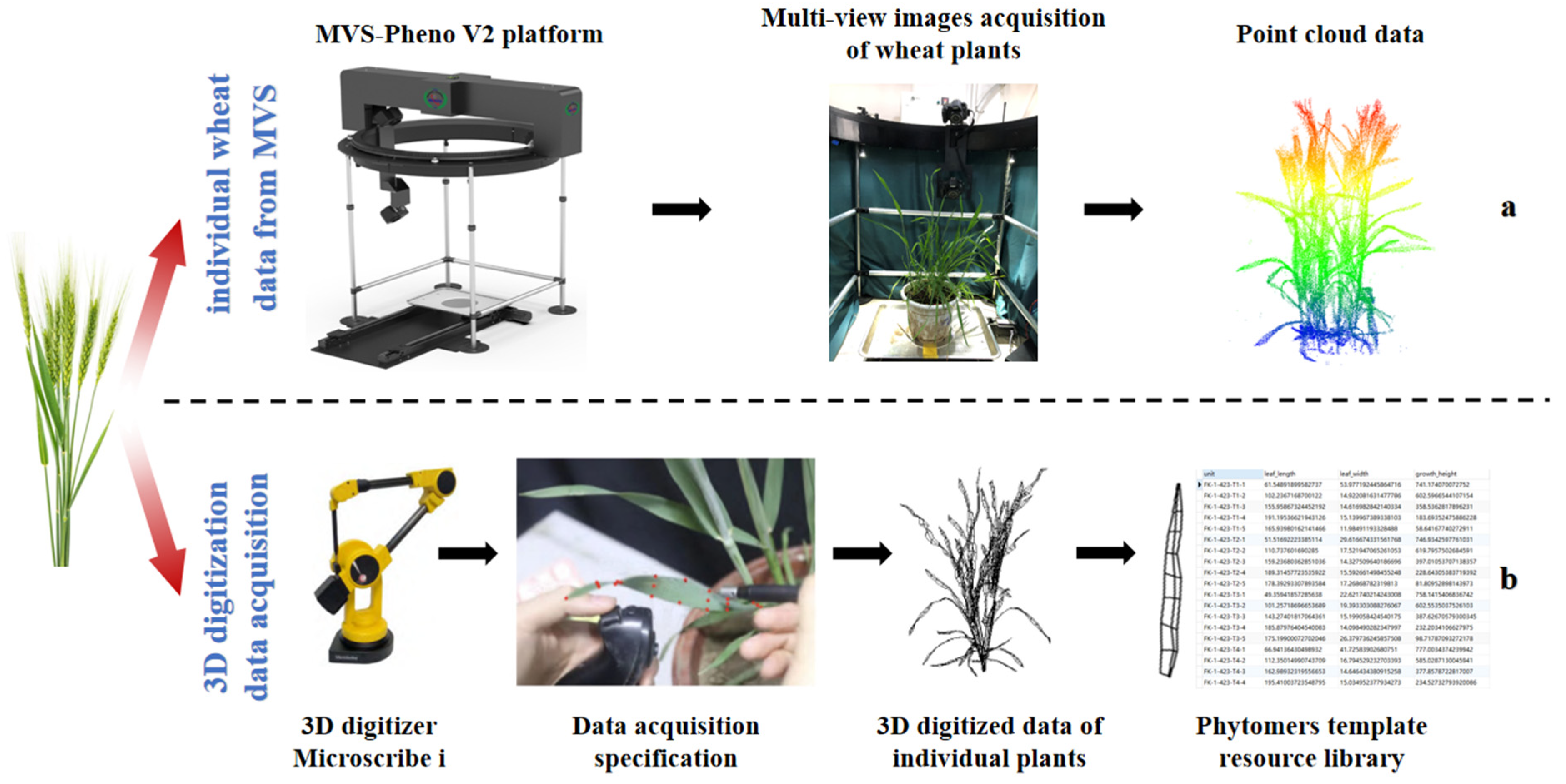
2.2. Data Acquisition

At the heading stage of wheat growth, three representative plants from each variety were carefully chosen as repeats to ensure that the sample plants had intact leaf surfaces. These plants were transplanted into pots and moved indoors. Initially, the multi-view imaging platform for plants MVS-Pheno V2 [32] was used to obtain multi-view images of each plant to obtain point cloud data of the plant as a whole. Subsequently, a 3D digitizer was used to obtain the 3D digitized data of plant organs [26] (Figure 1).

2.2.1. Acquisition of Multi-View Image Data for Plants

The MVS-Pheno V2 [32] phenotyping platform consists of two Canon cameras (Canon EOS 400D from Canon, Tokyo, Japan; the image resolution is 3888 × 2592), brackets for the cameras, and a distributed data acquisition controller, with one camera in each bracket, and a total of two brackets around the plant. The platform is capable of acquiring plant images from 64 different angles within 1 min, and can avoid 3D reconstruction errors caused by light changes or plant shaking during the process of photographing the same plant. The overlap rate of images taken from two adjacent angles is more than 75%, which ensures the quality of the 3D reconstructed point cloud.

2.2.2. Acquisition of 3D Digital Data for Plant Sub-Organs

The process of acquiring 3D digitized data for plants and sub-organs was carried out using a digitizer that can effectively acquire data within a range of 1.27 m with an accuracy of 0.178 mm, thus satisfying the requirements for acquiring 3D data of wheat plants. The data acquisition took place indoors in a windless environment, following a data acquisition standard [26]. Before acquiring data, the position was calibrated using a calibration block, and the plants were placed within the digitizer’s reachable distance. Three-dimensional phytomers [27] were employed as the basic acquisition unit, and the data acquisition of the entire plant was finalized by acquiring individual stems one by one. To ensure that all plant organs were under the same coordinate system, it was crucial not to move the plant during data acquisition. To avoid data errors resulting from variations in leaf location during data acquisition, the acquired data for each wheat stem were visualized and checked using supporting software (Rhino 6.0). Any loss or errors were then promptly corrected by reacquiring the data to validate their accuracy. During the process of acquiring 3D digitized data for plants, the individual stems were acquired in a specific order from outer to inner sections.

2.3. Data Processing

The multi-view image data of wheat plants captured by MVS-Pheno V2 [32] and the accompanying software can be utilized to reconstruct the dense 3D point cloud of each wheat plant. The acquired point clouds were simplified using space sampling with the sampling distance set to 0.5. Subsequently, the automatic identification of pots was used to remove the pots and obtain 3D point clouds of wheat plants. After applying statistical filtering to remove noise, a clean point cloud of the plant was obtained. To ensure computational efficiency, the uniformly down-sampled point cloud was used as input and constraints for the subsequent reconstruction.

The deep learning-based point cloud segmentation method [33] for wheat organs allows for the estimation of plant height, number of single stems, length of single stem, inclination and azimuth of single stems, and number of leaves on each single stem from the point cloud of wheat plants as driving parameters in reconstruction. These traits are then used as the driving parameters for reconstruction. However, the segmentation method is insufficient in its ability to extract organ-scale phenotypes due to the complex morphology and structure of wheat and internal occlusion issues. Furthermore, it is unable to extract all relevant morphological parameters required for 3D reconstruction, such as leaf length, leaf width, leaf azimuth, and inclination angle. Considering this, a virtual design-based 3D reconstruction approach is proposed to cater to the needs of 3D phenotyping and reconstruction of wheat plants.

In accordance with the standard for acquiring 3D digitized data for wheat [26], we conducted data standardization and extracted morphological parameters at varying scales. Specifically, we extracted plant height, stem length, single-stem azimuth, and inclination at the individual plant scale using the 3D digitized data. Additionally, we extracted leaf growing height, length, width, azimuth, and inclination at the phytomer scale. The given morphological and structural parameters of every 3D phytomer and digitized templates were amalgamated to form a database of wheat 3D phytomer templates [34]. This database served as the foundational data for all future reconstruction endeavors (Figure 1).

2.4. Initial Single-Stem 3D Model Construction

A wheat single-stem (main stem or tillers) model was created initially, with reference to the maize 3D modelling method that is based on the t-distribution function [13]. The number of phytomers on a single stem is represented as n. Samples of leaf length, maximum leaf width, leaf inclination angle, and leaf growth height are taken from the pre-modelled variety of wheat to model t-distribution probability density functions with n − 1 degrees of freedom, denoted as f(t):

$$f\left(t\right)=\frac{\Gamma \left(\frac{n}{2}\right)}{\sqrt{\left(n-1\right)\pi }\Gamma \left(\frac{n-1}{2}\right)}{\left(1+\frac{t^2}{n-1}\right)}^{-\frac{n}{2}},-\infty <t<\infty$$

Using leaf length as an example, a probability density distribution function was modelled within a 95% confidence interval from leaf length samples of several phytomers. Based on this distribution function, a random number of leaf lengths for each phytomer within the initial wheat model was generated.

Randomly generating the morphological and structural parameters of each phytomer on every single stem under corresponding t-distribution constraints guaranteed that modelling depicted some of the plant architecture characteristics unique to the existing wheat variety. The similarity metric function of a particular wheat variety was produced based on the sequence of leaves, leaf length, and inclination, and is used for matching with the optimal phytomer template in the database [13]:

$$E_i=a_c||c_i-c||+a_n\frac{||j_i-j||}{2.0}+a_{\phi }\frac{||{\phi }_i-\phi ||}{45.0}+a_l\frac{||l_i-l||}{100.0}$$

$$a_c+a_n+a_{\phi }+a_l=1$$

where c represents the variety name and One-Hot Encoding was used to deal with it, j denotes the leaf sequence, φ represents the leaf inclination angle, and l refers to the leaf length. For the i-th phytomer template, c_i, j_i, φ_i, and l_i represent the corresponding variety name, leaf sequence, leaf inclination angle, and leaf length, respectively. The denominators were determined through practical analysis. Additionally, a_c, a_n, a_φ, and a_l denote the coefficients of the parameters, respectively. The 3D phytomer that minimizes E_i was chosen as the template from the wheat phytomer 3D template database.

The phytomer template was then assembled based on the generated leaf inclination angle φ_i and growing height h_i to create the initial wheat single-stem model. Specifically, the given method involves rotating a phytomer template based on its azimuth and then translating it to its growth height. The azimuth and growth height parameters were generated using the t-distribution function. By transforming several selected phytomer templates, a single stem can be assembled.

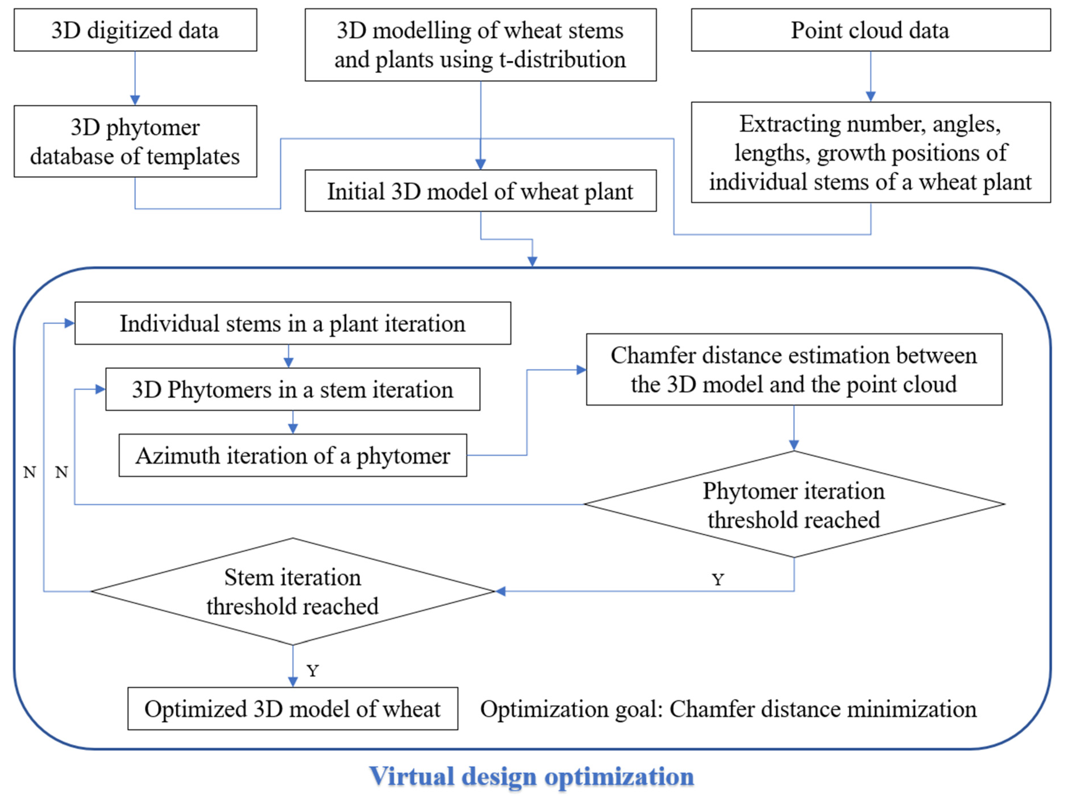
2.5. 3D Reconstruction of Wheat Plants by Virtual Design Optimization

The idea behind the virtual design-based 3D reconstruction approach for wheat plants is that numerous 3D models of wheat plants can be virtually created using the 3D phytomer templates in conjunction with the plant parametric modelling technique. These virtually constructed 3D plant models are then compared to the reconstructed input plant point cloud to identify the most comparable plant as the reconstruction outcome (Figure 2). Specifically, the initial 3D plant model was constructed by utilizing 3D digitized data to construct a 3D phytomer template database. The plant point cloud data was used to determine the constrain variables of each stem. The t-distribution method was then applied to combine the extracted data for the creation of the model. Based on this, the Chamfer distance (CD) was calculated between the designed 3D plant model and the initial point cloud. This was achieved by iterating the azimuth of single stems and 3D phytomers on the plant one by one. And finally, the reconstruction results were obtained for the target plant. Though time-consuming, the algorithm demonstrates good robustness and the process does not require manual interaction, leveraging the advantages of automatic computer calculation.

2.5.1. Initial Growth Position Extraction of Single Stems

The initial growth position of each stem on the plant determines the plant’s compactness and the distribution status of the stems, which significantly affects the accuracy of 3D wheat plant reconstruction. To ensure accuracy, growth position and distribution information of each stem at the base of the plant were extracted from the plant point cloud.

The point cloud of the plant was cut at a 10 cm height along the Z-axis from the root. These plant base point sets were clustered with a clustering algorithm. The smaller clusters were then removed as noise and then projected onto the XY-plane for the calculation of single-stem distribution density. To cluster the point cloud of the plant base, the KD-tree algorithm [35] was specifically used (Figure 3). During clustering, KD-tree may be deployed to partition point cloud data into similar feature subsets, which in turn facilitates clustering. The central point of each subset was calculated and projected onto the 2D plane, recorded as $p_k, 1\le k\le m$, which determined the growth point of each single stem within the plant (Figure 3). Based on the distribution of these m 2D plane points, n points were generated as the initial growth points of each single stem, where n is the number of single stems in the current plant.

2.5.2. Virtual Design and 3D Reconstruction of Wheat Plants

The parametric modelling method for plants, known as virtual plant design [11], creates 3D plant models with distinct morphology and structures by modifying the plants’ structural parameters and features on computers. For instance, the plant’s height can be altered by adjusting the internode’s length in combination with 3D scaling. Furthermore, the angle of the leaf blade can be modified by changing the azimuth of the blade along with 3D rotation. Finally, mesh deformation is utilized to modify the position of the characteristic points of the leaf veins to achieve a 3D leaf shape.

For the virtual modelling of wheat plants, the point cloud was used to determine the number of single stems, as well as their respective angles, lengths, and the number of leaves on each stem. Furthermore, the 3D phytomer template includes the inclination angle of the leaves as a varietal attribute. Thus, it is essential to ascertain the azimuth angle of the leaves on the phytomer, as adjusting it significantly affects the plant’s 3D spatial arrangement. Therefore, this paper focuses on the virtual design by iteratively adjusting the leaf azimuth angle to obtain single stems and individual plants. The reconstruction result is determined by calculating the similarity with the input plant point cloud, and selecting the 3D model that best matches the plant point cloud among all the virtually designed plants.

In the digital design process of wheat plant, the amount of single stems (n) is initially obtained through point cloud extraction. The 3D model of n single stems is then created via the single-stem 3D modelling process mentioned earlier. The single stems are subsequently translated and rotated according to each respective growth point and inclination angle extracted via point cloud, leading to the generation of the 3D model of the plant.

After obtaining the initial 3D model of the wheat plant, we conducted iterations of 3D phytomer azimuths to realize the virtual design. The outer single stem and its 3D phytomers are more deterministic in terms of space occupation, so we followed a clockwise iteration order with the outer single stem taking precedence. Additionally, we iterated the phytomers from top to bottom on the single stems (Figure 4).

The process of adjusting azimuths of 3D phytomers through a virtual design approach is explained as follows. The initial wheat mesh W model is viewed as a collection of individual single-stem models, denoted as W = {T₁, T₂, …, T_n}. The wheat single stems are positioned in an order that follows the aforementioned rule as the set W is traversed. Consider the initial wheat single-stem mesh model T as a set that comprises 3D phytomers u_i; that is, T = {u₁, u₂, …, u_m}. Traverse the T set in a top-to-bottom sequence, and then rotate each phytomer u_i counterclockwise around the vector v of the single stem in which it is located, in which the vector v is the single-stem vector.

Any unit vector a that is not parallel to v is chosen. Then, another unit vector b that is not parallel to v and a is obtained by taking the cross product of a and v. Use a, b, and v as the basis vectors for the new coordinate system and create the rotation matrix R. The unit vectors a, b, and v are the column vectors of R. Multiply the rotation matrix R by the matrix R_Z to obtain the final rotation matrix R_v which is rotated by θ counterclockwise around the vector v.

$$R=\left[\begin{array}{ccc}a\left[0\right]& v\left[0\right]& b\left[0\right]\\ a\left[1\right]& v\left[1\right]& b\left[1\right]\\ a\left[2\right]& v\left[2\right]& b\left[2\right]\end{array}\right]$$

$$R_Z=\left[\begin{array}{ccc}1& 0& 0\\ 0& \cos \theta & -\sin \theta \\ 0& \sin \theta & \cos \theta \end{array}\right]$$

$$R_v=R\times R_Z$$

The angle of rotation, θ, went from 0° to 360° in increments of 10°, and thus the number of iterations for each phytomer was 36 (refer to Figure 5). After each treatment, the 3D phytomers were returned to their corresponding place in set T, arranged in order, and then made into a temporary, single-stem set T^t. T^t then replaced the original single-stem set T in the current treatment to produce a temporary single-stem wheat set W^t = {T₁^t, T₂^t,…, T^t, …, T_n}.

In this study, the CD was utilized to measure the similarity between the point clouds P and the temporary individual plant mesh model W_t. In 3D space, the CD is defined as:

$$d_{CD}\left(P,W_t\right)=\frac{1}{P}{\displaystyle \sum }_{xϵP}\underset{yϵw}{\min }||x-y|{|}_2^2+\frac{1}{W_t}{\displaystyle \sum }_{yϵw}\underset{xϵP}{\min }||y-x|{|}_2^2$$

After each iteration, the current 3D model of the plant is compared to the input point cloud data using the CD, and the leaf azimuths of the 3D phytomers in each individual stem are recorded. Once all iterations of the current single stem have been completed, the optimized azimuth for this iteration is identified from the azimuth data of each 3D phytomer corresponding to the smallest CD. Additionally, the final position of the current phytomers u_i is determined by the azimuth φ corresponding to the rotation around v. The 3D reconstruction of the plant is accomplished by iterating through the initial set W until every single stem is iterated. The pseudo-code for this process is provided in Algorithm 1.

Algorithm 1. Virtual design to adjust the angle of Phytomers

Procedure: VIRTUALDESIGN(P,W)   1: for all tillerings Ti in W do   2:    for all units ui in T do   3:    for sita in range (0,360,10) do   4:      Set qj ← R(ui, sita)   5:      Set Tt ← ul, u2, …, gj, …, um   6:      Set W ← T1, T2, …, Tt, …,Tn   7:      Set N ← Hausdorff(P,W)   8:    end for   9:     Set fi ← 10*(index(argmin(N)) + 1)  10:     Set ui ← R(ui, fi)  11:   end for  12: Determine T such that T = ul, u2, …, un  13: end for  14: Determine W such that W = Tl, T2, …,Tn  15: return W

2.6. Evaluating Running Efficiency

As the running time is important for practical use, we also evaluated the efficiency of the method. The present methodology cannot be achieved in real time as it necessitates carrying out an extensive number of iterative computations to determine the CD between the mesh and the input point cloud. The evaluation was conducted by utilizing an Intel (R) Core (TM) i7-10700 CPU @2.90GHz computer with 16GB RAM.

2.7. Validation Methods

The accuracy of the proposed 3D reconstruction method for wheat plants is assessed by computing the Hausdorff distance between the input wheat plant point cloud data P and the reconstructed 3D mesh model W. This measure describes the degree of similarity between two point sets. The Hausdorff distance is defined as the maximum distance between any point in point cloud P and its nearest point in another point cloud, which is considered to be the set of vertices in mesh W. This distance is bi-directional and is defined by two sets of sets—P and W. The one-directional Hausdorff distance between these two sets of points is calculated.

$$h\left(P,W\right)=\underset{p\in P}{\max } \underset{w\in W}{\min }||p-w||$$

$$h\left(W,P\right)=\underset{w\in W}{\max } \underset{p\in P}{\min }||w-p||$$

The degree of similarity between two point sets is measured by the bi-directional Hausdorff distance, which takes the maximum of the one-directional Hausdorff distances. The higher the degree of matching, the smaller the bi-directional Hausdorff distance.

$$\mathrm{Hausdorff}\left(W,P\right)=\underset{ }{\max }\left\{h\left(P,W\right),h\left(W,P\right)\right\}$$

Furthermore, using the 3D digitized data collected in-site for each plant, we calculated 4 phenotypic traits: the plant height, crown width, total leaf area, and plant cover of each wheat plant. These four phenotypic indicators were then employed to verify the accuracy of the mesh model reconstructed from the wheat point cloud input. Plant height was measured as the difference between the Z-axis distance from the lowest to the highest point in the dataset. Crown width was measured as the straight-line distance between the two farthest points after the data were projected onto the XY plane. Plant leaf area was computed as the sum of all triangular facets of the mesh model, and plant coverage was obtained by dividing the plant area projected onto the XY plane by an area of a square with sides length of 1.0 m. The R², root mean squared error (RMSE), and Normalized Root Mean Squared Errors (NRMSE) were computed.

$$\overline{x}=\frac{1}{n}{\displaystyle \sum }_{i=1}^n{x}_i$$

$$R^2=1-\frac{{{\displaystyle \sum }}_i{\left(x_i-{\widehat{x}}_i\right)}^2}{{{\displaystyle \sum }}_i{\left(x_i-\overline{x}\right)}^2}$$

$$\mathrm{RMSE}=\sqrt{\frac{1}{n}{\displaystyle \sum }_{i=1}^n{\left({\widehat{x}}_i-x_i\right)}^2}$$

$$\mathrm{NRMSE}=\frac{1}{\overline{x}}\sqrt{\frac{1}{n}{\displaystyle \sum }_{i=1}^n{\left({\widehat{x}}_i-x_i\right)}^2}\times 100\%$$

where $x_i$ represents the phenotypic parameter extracted from the $i$-th generative model, and ${\widehat{x}}_i$ represents the phenotypic parameter extracted from the point cloud. The number of samples is n, while RMSE and NRMSE indicate the error between each phenotypic parameter calculated in the model and those of the actual plants.

To evaluate the consistency between the reconstructed 3D model and the input plant point cloud in 3D space, the reconstructed mesh model was converted into another point cloud and uniformly down-sampled. The two point clouds were divided into five layers each based on plant height. The percentage of point density in each layer was then compared. The Mean Absolute Percentage Error (MAPE) was computed for every dataset group.

$$\mathrm{MAPE}=\frac{1}{n}{\displaystyle \sum }_{i=1}^n{\left({\widehat{y}}_i-y_i\right)}^2\times 100\%$$

3. Results

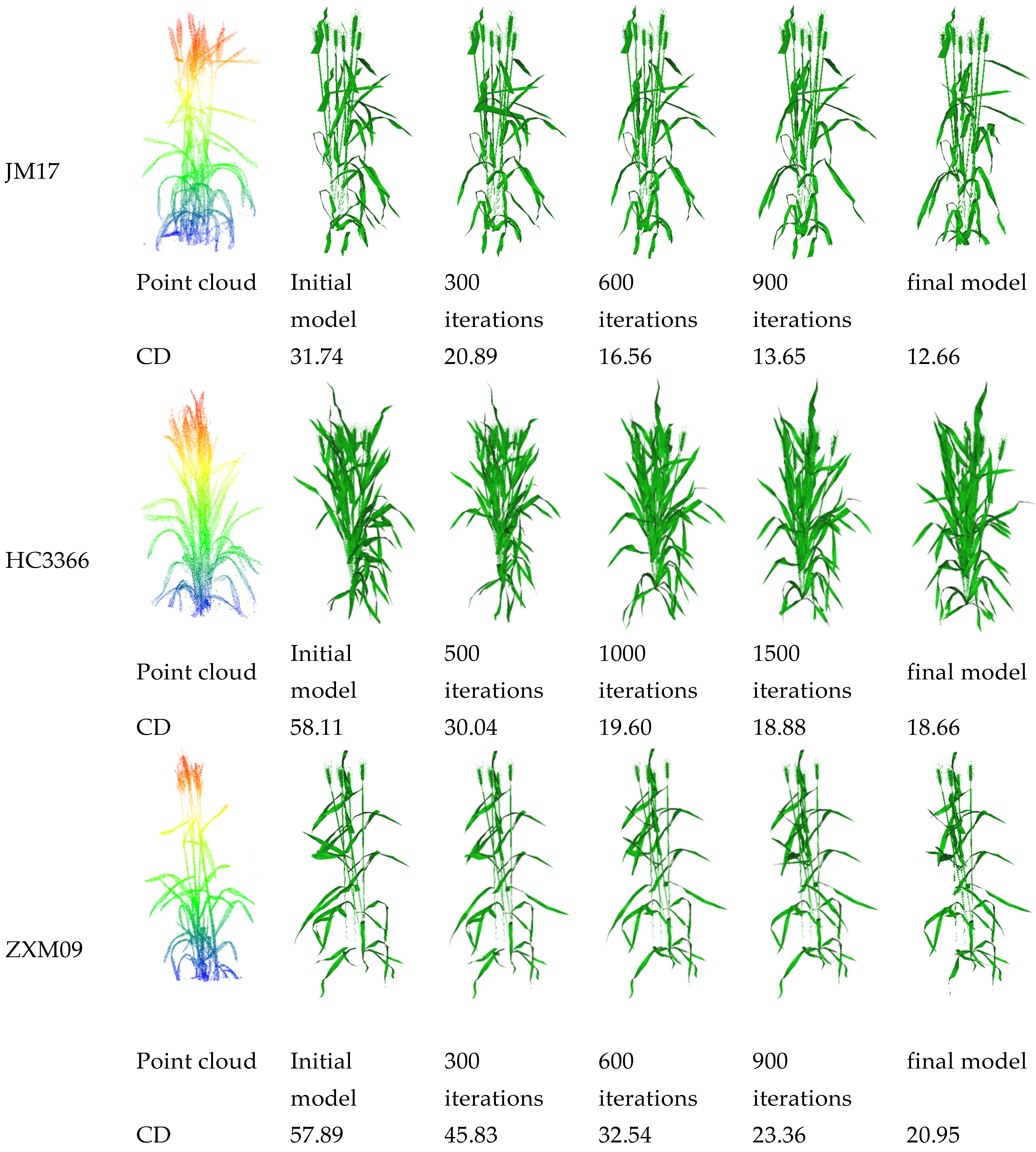
3.1. Visualization Results of 3D Reconstructed Plants

The described approach was utilized to reconstruct 3D models of the flowing stage plants among the nine wheat cultivars acquired. The visualizations of the reconstructions for each variety can be observed in Figure 6. Based on the visualization results, the method is mostly effective in presenting the 3D morphology of plant varieties in relation to plant architecture, such as the plants’ compactness and the height-wise distribution of leaves. Despite the method not producing an exact match to the original input point cloud, it still exhibits significant differences.

Three individual plants of each wheat variety were reconstructed utilizing the 3D modeling method mentioned earlier using the collected plant point cloud data. The 3D models of wheat populations for nine different varieties were further generated, taking into account the settings for the population row spacing and the rotation of each plant at random angles. Each population consisted of a total of nine plants, arranged in three rows by three plants. The plant spacing was 0.05 m and the row spacing was 0.3 m. From the population visualization results shown in Figure 7, it can be observed that the 3D models constructed for different wheat varieties exhibit distinguishable variations in plant and canopy architecture. Such models can be utilized for further 3D visualization purposes like canopy light distribution and plant architecture analysis.

3.2. Verification Results

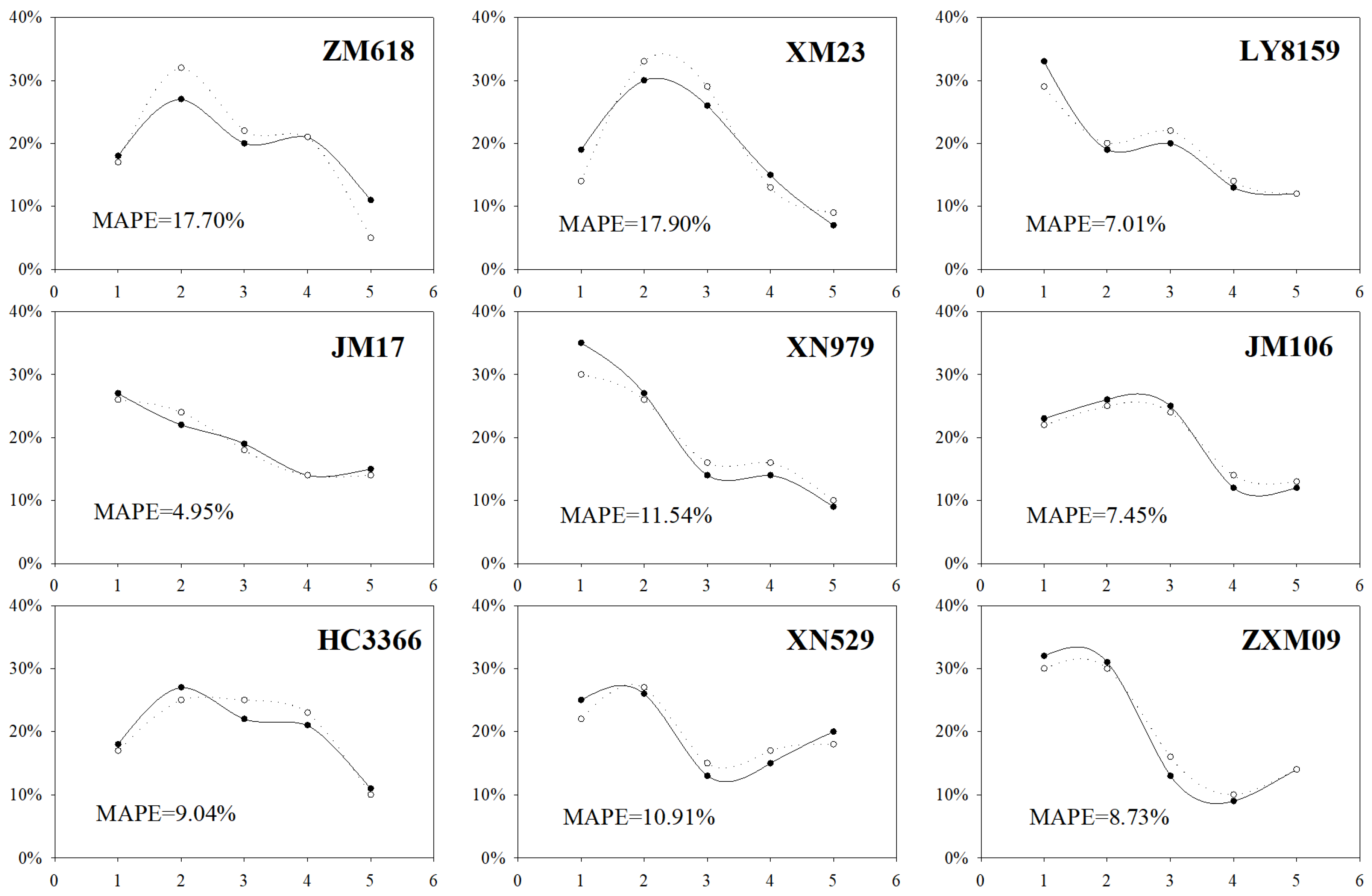
3.2.1. Comparative Validation of Plant Phenotypes

As each input point cloud for each plant had corresponding initial 3D digitized data, we were able to extract information such as plant height, crown width, plant leaf area, and coverage using these data. We then used the 3D reconstruction results to extract the corresponding plant phenotypic parameters for comparative validation, as shown in Figure 8. The reconstruction results of the 27 plants were used to calculate the R², RMSE, and NRMSE for four plant phenotypic parameters. SPSS and PP-plots were used to test for normality. The data were found to conform to a normal distribution. The R² values were 0.80, 0.73, 0.90, and 0.69 for plant height, crown width, plant leaf area, and plant coverage, respectively. The RMSE values were 4.56 cm, 3.85 cm, 295.44 cm², and 5.77% for plant height, crown width, plant leaf area, and plant coverage, respectively. The NRMSE values were 0.10, 0.12, 0.08, and 0.17 for the same parameters. The most successful reconstructions were achieved for plant leaf area, primarily due to the use of the 3D template of the targeted variety’s phytomers, with only small variations in leaf area among the different 3D phytomers. The following most effective result was the plant height. In reality, the method’s iteration led to minimal changes in the plant’s leaf area and height, mostly due to the primary rotation of the leaves on the 3D phytomers. Even though leaf rotation, obtained through the iteration of the phytomers, had a larger impact on crown width and plant coverage, the discrepancies between plants were more significant. As a result, the R² and NRMSE were lower for leaf rotation compared to plant height and leaf area. Despite this, the numerical outcomes of all four plant parameters were satisfactory, signifying that the reconstruction results were in good concordance with the measured data.

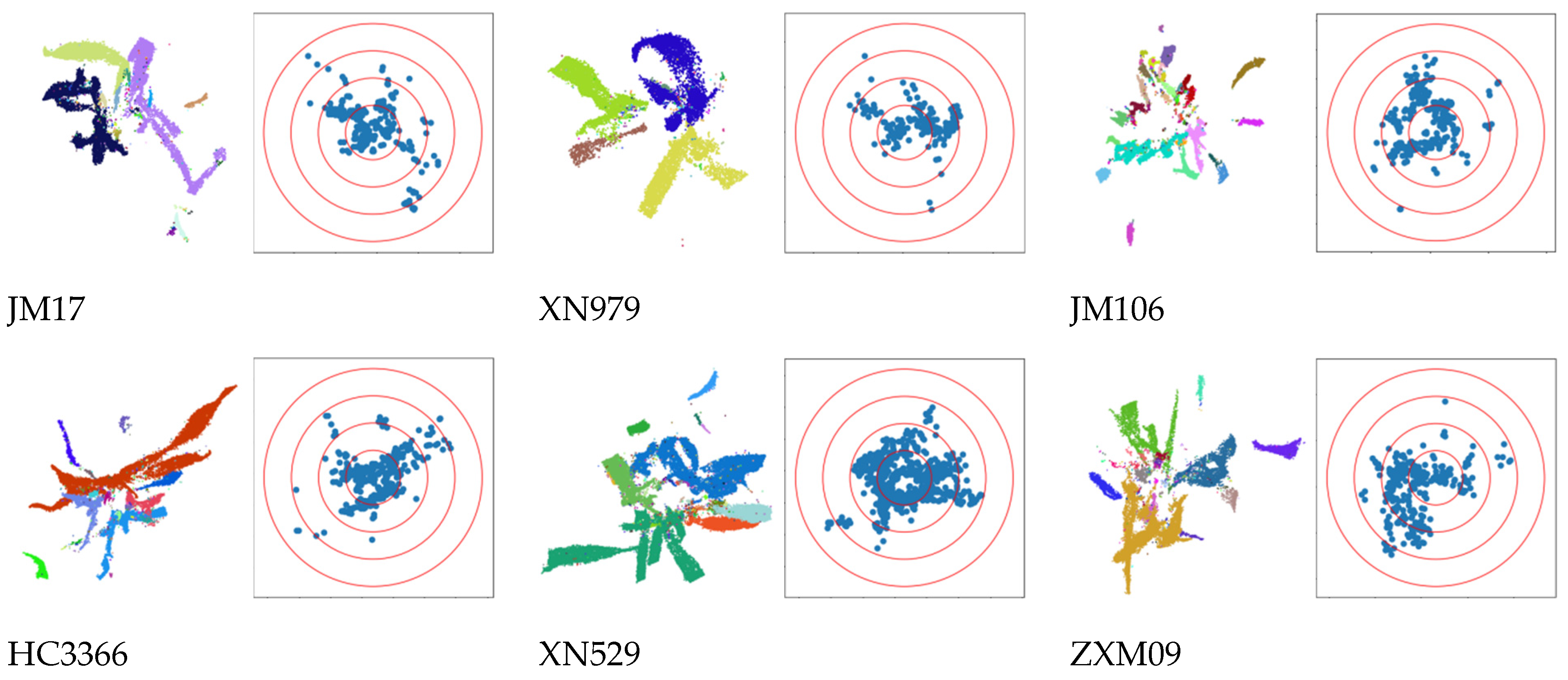
3.2.2. Comparison of Spatial Distribution of Reconstruction Results

To assess the correlation between the reconstructed 3D plant model and the input point cloud in 3D spatial distribution, the wheat point cloud and corresponding plant model were uniformly down-sampled and sliced into five layers based on the plant height from low to high. The MAPE was computed to compare the point density proportion across each layer, and the results are displayed in Figure 9. The MAPEs for the JM17 and JM106 varieties were relatively low at 4.59% and 7.01%, respectively, indicating that the model reconstruction accuracy was higher for these two varieties. The MAPEs for ZM618 and XM23 were higher at 17.70% and 17.90% than other varieties, respectively, whereas the other varieties’ MAPEs were within the range of 4.95% to 11.54%. The reconstructed 3D models of all varieties of wheat plants displayed consistent curve trends regarding vertical spatial distribution with the input point cloud. The MAPE values were small, indicating that the method can be relied upon to reconstruct 3D models of plants that accurately reflect varietal plant architecture and spatial distribution. This capability satisfies the needs of functional–structural analysis of wheat varieties.

3.2.3. Hausdorff Distance between Plant Point Cloud and Reconstructed 3D Models

The Hausdorff distance is a tool utilized for determining the maximum distance between two sets, predominantly employed to evaluate the similarity between the reconstructed model and the 3D point cloud. As the Hausdorff distance becomes smaller, the point clouds become more alike, and the reconstruction accuracy increases correspondingly. The data shown in Figure 10 illustrate that the Hausdorff distances for 27 plants of the nine different varieties measured were between 20.16 and 39.41 cm. Due to the non-1:1 reconstruction, the Hausdorff distances are larger than those of accurate reconstructions. When examining the distribution of point clouds in vertical space alongside the aforementioned information, it becomes clear that while the general spatial distribution aligns with the input point cloud, the maximum distance reflected by the Hausdorff distance highlights significant discrepancies in certain aspects of the reconstruction. The approach uses CD to attain the minimum average distance of the reconstruction outcome as a whole, which is unavoidably compromised in the specific points, and this is a significant starting point for advancing the method’s precision.

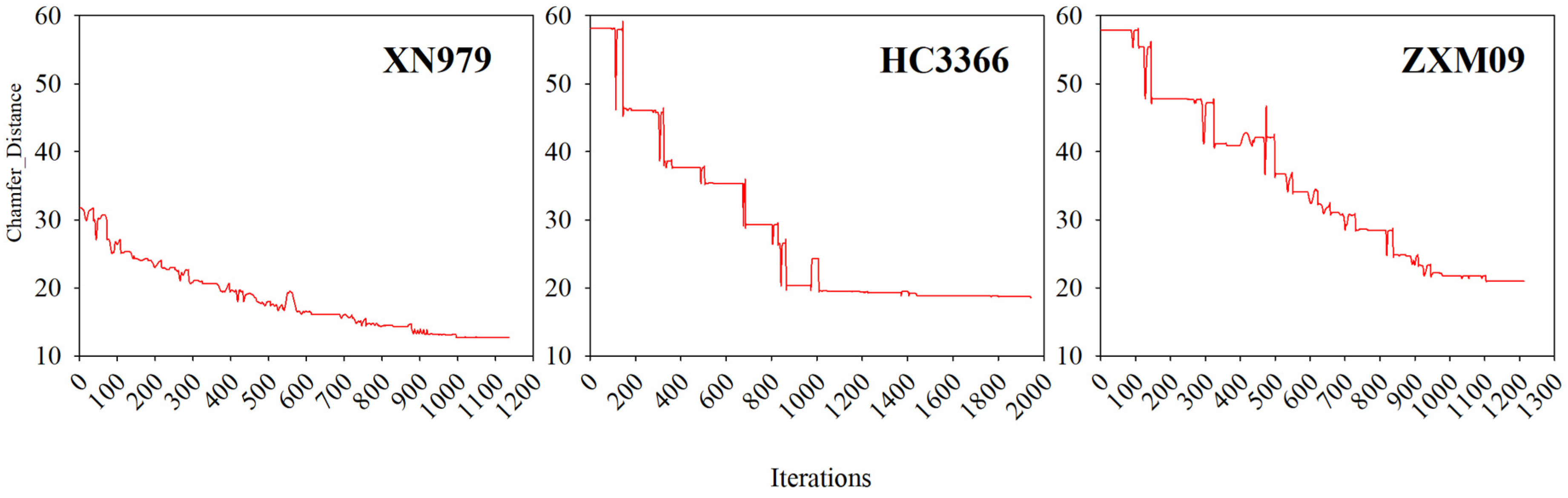
3.3. Iteration Process

For a more intuitive optimization process of the virtual design method, the CD variation during the iteration and the visualization of the intermediate plant results were shown using three wheat cultivars: JM17, HC3366, and ZMX09, which differ significantly in plant architecture. The azimuth step for each iteration was set at 10°. Figure 11 illustrates the trends in CD variation between the virtually designed 3D model of the wheat plant and the corresponding input point cloud during the iteration. The overall decreasing trend for each variety confirms that the 3D model gets closer to the plant point cloud as the 3D plant model continuously adjusts, demonstrating the effectiveness of the method. The rate of decline was greater at the start of the iteration, with a more gradual decrease towards the end before ultimately stabilizing. Similar trends have been observed in other varieties. Additionally, the variation curves frequently exhibit horizontal alterations, mainly caused by the slight rotation angle of individual 3D phytomers during processing, resulting in minor fluctuations in CD.

Figure 12 illustrates the gradual process of obtaining the final wheat model from the initial 3D model by iterations for the three wheat plant varieties and their corresponding CD variations. The number of iterations per phytomer is 36, and thus the number of iterations for each variety depends on the total number of 3D phytomers, which varies. The visualization results indicate that the initial constructed 3D models are already consistent with the input point cloud to some extent. This is due to constraint information, including the number, length, and inclination of each single stem and their initial growth position extracted from the point cloud. Additionally, 3D phytomer templates of the current varieties were employed. During the following iterations, the 3D model of the plant was approaching the original point cloud data of the plant, with particular improvement in the spatial distribution of certain organs. This further demonstrates the efficacy of the approach.

3.4. Running Efficiency

Table 2. Method efficiency.

Variety	Number of Points after Uniform Down-Sampling	Number of Single-Stems	Number of Phytomers	Time Cost Using 5° Iteration Step (s)	Time Cost Using 10° Iteration Step (s)	Time Cost Using 20° Iteration Step (s)
XN979	3556	7	31	1003.27	498.34	239.33
HC3366	4045	11	54	2191.31	1088.02	598.15
ZXM09	3603	7	32	1123.59	553.24	270.12

presents the quantity of point cloud data for each plant, using uniform voxel down-sampling parameters. Additionally, it provides information on the individual single-stems, the number of 3D phytomers, the number of iterations performed at varying angles, and the time cost of the reconstruction process for the three plant varieties mentioned. The results reveal that the running time of the technique and azimuth iteration step share a negative correlation. Moreover, as the number of points in the point cloud and phytomers increases, the execution time of the technique also increases in a multiplicative manner. The running time was mainly influenced by the number of phytomers in a single stem, so there seems to be no correlation between the number of single stems and the density of phytomers on a single stem varied between species. Hence, the quantity of points present in the input plant point cloud, the number of 3D phytomers, and the length of the iteration step collectively impact the execution time of the technique.

4. Discussion

Wheat is among the world’s three primary grain crops, and wheat plant architecture plays a significant role in wheat breeding, cultivation research, and production. Currently, the methods for observing wheat plant architecture mainly rely on manual measurement and counting, which fails to accurately depict the 3D spatial morphology and structure distinctions amongst various varieties and cultivation techniques. Consequently, such approaches cannot fulfil the requirement for high-throughput phenotyping of vast quantities of breeding materials [36]. Wheat crops possess numerous and closely spaced tillers that bring about substantial overlaps between organs, rendering it arduous to apply standardized 3D reconstruction techniques commonly employed in crop analysis. This poses challenges in solving the problem of 3D reconstruction and phenotyping of wheat plants. LiDAR or multi-view 3D reconstruction techniques [32] can be applied to gather 3D point cloud data on the exterior of the wheat plant. However, the resulting point cloud is severely limited due to organ occlusion, elongated leaves and stems, and subtle color differences between organs. This presents a significant challenge to robustly and accurately segmenting single stems and organs from the complex point cloud. For this reason, researchers have mainly undertaken 3D reconstruction of wheat organs [25], or early plants with simpler structures [28], or used 3D modelling methods to simulate plants [26,27]. Achieving 3D reconstruction of wheat plants with different growth stages and varietal plant architectures using 3D point clouds has consistently presented a challenging issue within the study of wheat plant architecture.

To address the issue of 3D reconstruction and phenotype extraction when utilizing wheat point cloud data, this study proposes a virtual design-based 3D reconstruction approach for wheat plants. The virtual design method utilizes a 3D phytomer template database with variety differences to provide morphological and structural data support. The input and constraint information are derived from the 3D point cloud. By utilizing the massive computational optimization searching capabilities, thousands of 3D wheat plant models are iteratively designed and the most similar model to the plant point cloud is identified as the reconstruction result. Though not a precise 1:1 reconstruction, the reconstructed model effectively represents the 3D spatial distribution characteristics and phenotypic traits of the target plant, such as plant height, crown width, leaf area, and coverage, from an individual plant perspective. Additionally, it depicts 3D spatial differences in plant architectures of different varieties. This method aims to improve consistency between the reconstruction models and the input point cloud in 3D space. However, the accuracy for the simplest plant height is not the highest. The main reason is that the determination of plant height is determined by the very few organs at the top of the whole plant. The method addresses the gap in 3D reconstruction methods for multi-tillering crop plants using point cloud data. Combined with the 3D phytomer [27] template reconstructed from high-quality point cloud [25] data, this method can be applied to the 3D reconstruction of wheat plants throughout their lifecycle and offers practical technical support for phenotype extraction of the wheat morphology and structure. Additionally, based on the reconstructed wheat mesh model, this method can be combined with canopy light distribution calculation approaches for functional–structural analysis. For instance, it can be used to analyze the radiation utilization efficiency of different wheat varieties and plant architectures [31].

Under the premise of having a varietal-resolution organ 3D template database, the virtual design-based 3D reconstruction method for plants is highly scalable and especially suitable for 3D reconstruction studies of plants with complex structures and incomplete point clouds. However, this method can only provide a 3D model that bears a close resemblance to the target plant with regard to the plant’s overall shape and spatial distribution. Achieving a 1:1 3D reconstruction is challenging, particularly when there are inadequate varietal organ templates available. In future work, we will incorporate and extract more morphological and structural knowledge into the 3D framework of wheat plants as constraints, which will narrow down the range of iterations in the virtual design and enhance the algorithm’s efficiency while ensuring the accuracy of reconstruction. Additionally, we will utilize this method in combination with the 3D plant phenotyping platform [32] to execute 3D reconstruction and phenotype extraction and analysis for numerous wheat varieties.

References

1. Bucksch, A.; Atta-Boateng, A.; Azihou, A.F.; Battogtokh, D.; Baumgartner, A.; Binder, B.M.; Braybrook, S.A.; Chang, C.; Coneva, V.; DeWitt, T.J.; et al. Morphological Plant Modeling: Unleashing Geometric and Topological Potential within the Plant Sciences. Front. Plant Sci. 2017, 8, 900. [Google Scholar] [CrossRef]
2. Yang, W.; Feng, H.; Zhang, X.; Zhang, J.; Doonan, J.H.; Batchelor, W.D.; Xiong, L.; Yan, J. Crop Phenomics and High-Throughput Phenotyping: Past Decades, Current Challenges, and Future Perspectives. Mol. Plant 2020, 13, 187–214. [Google Scholar] [CrossRef]
3. Henke, M.; Kurth, W.; Buck-Sorlin, G.H. FSPM-P: Towards a general functional-structural plant model for robust and comprehensive model development. Front. Comput. Sci. 2016, 10, 1103–1117. [Google Scholar] [CrossRef]
4. Louarn, G.; Song, Y. Two decades of functional–structural plant modelling: Now addressing fundamental questions in systems biology and predictive ecology. Ann. Bot. 2020, 126, 501–509. [Google Scholar] [CrossRef] [PubMed]
5. Okura, F. 3D modeling and reconstruction of plants and trees: A cross-cutting review across computer graphics, vision, and plant phenotyping. Breed. Sci. 2022, 72, 31–47. [Google Scholar] [CrossRef] [PubMed]
6. Gibbs, J.A.; Pound, M.; French, A.P.; Wells, D.M.; Murchie, E.; Pridmore, T. Approaches to three-dimensional reconstruction of plant shoot topology and geometry. Funct. Plant Biol. 2017, 44, 62–75. [Google Scholar] [CrossRef] [PubMed]
7. Karwowski, R.; Prusinkiewicz, P. The L-system-based plant-modeling environment L-studio 4.0. In Proceedings of the 4th International Workshop on Functional-Structural Plant Models, 2004, UMR AMAP, Montpellier, France, 7–11 June 2004; 2004. [Google Scholar]
8. Hemmerling, R.; Evers, J.B.; Smoleňová, K.; Buck-Sorlin, G.; Kurth, W. Extension of the GroIMP modelling platform to allow easy specification of differential equations describing biological processes within plant models. Comput. Electron. Agric. 2013, 92, 1–8. [Google Scholar] [CrossRef]
9. Winiwarter, L.; Pena, A.M.E.; Weiser, H.; Anders, K.; Sanchez, J.M.; Searle, M.; Höfle, B. Virtual laser scanning with HELIOS plus plus: A novel take on ray tracing-based simulation of topographic full-waveform 3D laser scanning. Remote Sens. Environ. 2022, 269, 112772. [Google Scholar] [CrossRef]
10. Kierzkowski, D.; Runions, A.; Vuolo, F.; Strauss, S.; Lymbouridou, R.; Routier-Kierzkowska, A.-L.; Wilson-Sánchez, D.; Jenke, H.; Galinha, C.; Mosca, G.; et al. A Growth-Based Framework for Leaf Shape Development and Diversity. Cell 2019, 177, 1405–1418.e17. [Google Scholar] [CrossRef] [PubMed]
11. Runions, A.; Tsiantis, M.; Prusinkiewicz, P. A common developmental program can produce diverse leaf shapes. New Phytol. 2017, 216, 401–418. [Google Scholar] [CrossRef] [PubMed]
12. Qian, B.; Huang, W.; Xie, D.; Ye, H.; Guo, A.; Pan, Y.; Jin, Y.; Xie, Q.; Jiao, Q.; Zhang, B.; et al. Coupled maize model: A 4D maize growth model based on growing degree days. Comput. Electron. Agric. 2023, 212, 108124. [Google Scholar] [CrossRef]
13. Wen, W.L.; Zhao, C.J.; Guo, X.Y.; Wang, Y.J.; Du, J.J.; Yu, Z.T. Construction method of three-dimensional model of maize colony based on t-distribution function. Trans. Chin. Soc. Agric. Eng. 2018, 34, 192–200. [Google Scholar]
14. Han, X.F.; Laga, H.; Bennamoun, M. Image-Based 3D Object Reconstruction: State-of-the-Art and Trends in the Deep Learning Era. IEEE Trans. Pattern Anal. Mach. Intell. 2021, 43, 1578–1604. [Google Scholar] [CrossRef] [PubMed]
15. Harandi, N.; Vandenberghe, B.; Vankerschaver, J.; Depuydt, S.; Van Messem, A. How to make sense of 3D representations for plant phenotyping: A compendium of processing and analysis techniques. Plant Methods 2023, 19, 60. [Google Scholar] [CrossRef]
16. Slattery, R.A.; Ort, D.R. Perspectives on improving light distribution and light use efficiency in crop canopies. Plant Physiol. 2021, 185, 34–48. [Google Scholar] [CrossRef] [PubMed]
17. Yin, K.; Huang, H.; Long, P.; Gaissinski, A.; Gong, M.; Sharf, A. Full 3D Plant Reconstruction via Intrusive Acquisition. Comput. Graph. Forum 2016, 35, 272–284. [Google Scholar] [CrossRef]
18. Zhu, T.; Ma, X.; Guan, H.; Wu, X.; Wang, F.; Yang, C.; Jiang, Q. A method for detecting tomato canopies’ phenotypic traits based on improved skeleton extraction algorithm. Comput. Electron. Agric. 2023, 214, 108285. [Google Scholar] [CrossRef]
19. Jin, S.; Sun, X.; Wu, F.; Su, Y.; Li, Y.; Song, S.; Xu, K.; Ma, Q.; Baret, F.; Jiang, D.; et al. Lidar sheds new light on plant phenomics for plant breeding and management: Recent advances and future prospects. ISPRS J. Photogramm. Remote Sens. 2021, 171, 202–223. [Google Scholar] [CrossRef]
20. Chaivivatrakul, S.; Tang, L.; Dailey, M.N.; Nakarmi, A.D. Automatic morphological trait characterization for corn plants via 3D holographic reconstruction. Comput. Electron. Agric. 2014, 109, 109–123. [Google Scholar] [CrossRef]
21. Zermas, D.; Morellas, V.; Mulla, D.; Papanikolopoulos, N. 3D model processing for high throughput phenotype extraction—The case of corn. Comput. Electron. Agric. 2019, 172, 105047. [Google Scholar] [CrossRef]
22. Sampaio, G.S.; Silva, L.A.; Marengoni, M. 3D Reconstruction of Non-Rigid Plants and Sensor Data Fusion for Agriculture Phenotyping. Sensors 2021, 21, 4115. [Google Scholar] [CrossRef] [PubMed]
23. Artzet, S.; Chen, T.W.; Chopard, J.; Brichet, N.; Mielewczik, M.; Cohen-Boulakia, S.; Cabrera-Bosquet, L.; Tardieu, F.; Fournier, C.; Pradal, C. Phenomenal: An automatic open source library for 3D shoot architecture reconstruction and analysis for image-based plant phenotyping. bioRxiv 2019, 805739. [Google Scholar] [CrossRef]
24. Ando, R.; Ozasa, Y.; Guo, W. Robust Surface Reconstruction of Plant Leaves from 3D Point Clouds. Plant Phenomics 2021, 2021, 3184185. [Google Scholar] [CrossRef] [PubMed]
25. Kempthorne, D.M.; Turner, I.W.; Belward, J.A.; McCue, S.W.; Barry, M.; Young, J.; Dorr, G.J.; Hanan, J.; Zabkiewicz, J.A. Surface reconstruction of wheat leaf morphology from three-dimensional scanned data. Funct. Plant Biol. 2015, 42, 444–451. [Google Scholar] [CrossRef] [PubMed]
26. Zheng, C.; Wen, W.; Lu, X.; Chang, W.; Chen, B.; Wu, Q.; Xiang, Z.; Guo, X.; Zhao, C. Three-Dimensional Wheat Modelling Based on Leaf Morphological Features and Mesh Deformation. Agronomy 2022, 12, 414. [Google Scholar] [CrossRef]
27. Chang, W.; Wen, W.; Zheng, C.; Lu, X.; Chen, B.; Li, R.; Guo, X. Geometric Wheat Modeling and Quantitative Plant Architecture Analysis Using Three-Dimensional Phytomers. Plants 2023, 12, 445. [Google Scholar] [CrossRef]
28. Duan, T.; Chapman, S.; Holland, E.; Rebetzke, G.; Guo, Y.; Zheng, B. Dynamic quantification of canopy structure to characterize early plant vigour in wheat genotypes. J. Exp. Bot. 2016, 67, 4523–4534. [Google Scholar] [CrossRef]
29. Wu, D.; Yu, L.; Ye, J.; Zhai, R.; Duan, L.; Liu, L.; Wu, N.; Geng, Z.; Fu, J.; Huang, C.; et al. Panicle-3D: A low-cost 3D-modeling method for rice panicles based on deep learning, shape from silhouette, and supervoxel clustering. Crop J. 2022, 10, 1386–1398. [Google Scholar] [CrossRef]
30. Liu, S.; Baret, F.; Abichou, M.; Boudon, F.; Thomas, S.; Zhao, K.; Fournier, C.; Andrieu, B.; Irfan, K.; Hemmerlé, M.; et al. Estimating wheat green area index from ground-based LiDAR measurement using a 3D canopy structure model. Agric. For. Meteorol. 2017, 247, 12–20. [Google Scholar] [CrossRef]
31. Barillot, R.; Chambon, C.; Fournier, C.; Combes, D.; Pradal, C.; Andrieu, B. Investigation of complex canopies with a functional–structural plant model as exemplified by leaf inclination effect on the functioning of pure and mixed stands of wheat during grain filling. Ann. Bot. 2019, 123, 727–742. [Google Scholar] [CrossRef]
32. Wu, S.; Wen, W.; Gou, W.; Lu, X.; Zhang, W.; Zheng, C.; Xiang, Z.; Chen, L.; Guo, X. A miniaturized phenotyping platform for individual plants using multi-view stereo 3D reconstruction. Front. Plant Sci. 2022, 13, 897746. [Google Scholar] [CrossRef] [PubMed]
33. Pengliang, X.; Sheng, W.; Shiqing, G.; Weiliang, W.; Chuanyu, W.; Xianju, L.; Xiaofen, G.; Wenrui, L.; Linsheng, H.; Dong, L.; et al. ICFMNet: An Automated Segmentation and 3D Phenotypic Analysis Pipeline for Plant, Spike, and Flag Leaf type of Wheat. Comput. Electron. Agric. 2024; under review. [Google Scholar]
34. Wen, W.; Wang, Y.; Wu, S.; Liu, K.; Gu, S.; Guo, X. 3D phytomer-based geometric modelling method for plants—The case of maize. AoB Plants 2021, 13, plab055. [Google Scholar] [CrossRef]
35. Yuan, X.; Liu, B.; Ma, Y. Anisotropic neighborhood searching for point cloud with sharp feature. Meas. Control 2020, 53, 1943–1953. [Google Scholar] [CrossRef]
36. Gao, J.; Hu, X.; Gao, C.; Chen, G.; Feng, H.; Jia, Z.; Zhao, P.; Yu, H.; Li, H.; Geng, Z.; et al. Deciphering genetic basis of developmental and agronomic traits by integrating high-throughput optical phenotyping and genome-wide association studies in wheat. Plant Biotechnol. J. 2023, 21, 1966–1977. [Google Scholar] [CrossRef] [PubMed]
Figure 1. Data acquisition process. (a) Point cloud data acquisition. (b) Three-dimensional digitized data acquisition.
Agriculture 14 00391 g001
Figure 2. Wheat single stem and individual plant modeling process.
Agriculture 14 00391 g002
Figure 3. Visualization results of initial growth position clustering of wheat plants using KD-tree (left) with the distribution of the centroids of each subset after projection on a 2D plane (right).
Agriculture 14 00391 g003aAgriculture 14 00391 g003b
Figure 4. Adjustment of the order of single stems on plants and of phytomers on single stems during the virtual design process. (a) Individual single-stem growth points on the plant extracted based on the basal point cloud projection. (b) Schematic diagram of the single-stem iteration sequence. (c) Schematic diagram of the 3D phytomer iteration sequence. The yellow dots in (a) and the green dots in (b) both indicate the growth position of each single stem, and the arrows point to the order of the iterations.
Agriculture 14 00391 g004
Figure 5. Front view (top) and top view (bottom) of rotating a phytomer interactively counter-clockwise by 72° around the single-stem vector.
Agriculture 14 00391 g005
Figure 6. Visualization of 3D reconstruction outcomes for various wheat plant architectures. The input point cloud data appear on the left-hand side for each type, while the reconstructed 3D mesh model appears on the right.
Agriculture 14 00391 g006aAgriculture 14 00391 g006b
Figure 7. Three-dimensional models of a 3 × 3 population of nine wheat varieties with 0.3 m row spacing and 0.05 m plant spacing.
Agriculture 14 00391 g007aAgriculture 14 00391 g007b
Figure 8. Comparison of the plant height, crown width, plant leaf area, and plant coverage estimated using the reconstructed model with the measured 3D digitized data.
Agriculture 14 00391 g008
Figure 9. Trend of the point density ratio (y-axis) between the down-sampled point cloud and the points in the down-sampled mesh model after dividing the points into five layers (x-axis) according to the plant height from low to high. The response point cloud P and response grid model w are depicted by solid and dashed lines respectively. The MAPE between the two point density curves are also given for each variety.
Agriculture 14 00391 g009
Figure 10. Hausdorff distance between the reconstructed 3D plant model and the corresponding plant point cloud.
Agriculture 14 00391 g010
Figure 11. Curve of CD variation during iteration of wheat plants of three varieties. The iterations of each cultivar are different, so the times of iteration in the X-axis are not the same.
Agriculture 14 00391 g011
Figure 12. Visualization of the iterative process of three varieties of wheat plants.
Agriculture 14 00391 g012