Enhancing Subsurface Soil Moisture Forecasting: A Long Short-Term Memory Network Model Using Weather Data

Abstract

Subsurface soil moisture is a primary determinant for root development and nutrient transportation in the soil and affects the tractability of agricultural vehicles. A statistical forecasting model, Vector AutoRegression (VAR), and a Long Short-Term Memory network (LSTM) were developed to forecast the subsurface soil moisture at a 20 cm depth using 9 years of historical weather data and subsurface soil moisture data from Fort Wayne, Indiana, USA. A time series analysis showed that the weather data and soil moisture have a stationary seasonal tendency and demonstrated that soil moisture can be forecasted from weather data. The VAR model estimates volumetric soil moisture of one-day ahead with an R², MAE (m³m⁻³), MSE (m⁶m⁻⁶), and RMSE (m³m⁻³) of 0.698, 0.0561, 0.0046, and 0.0382 for 2021 corn cropping season, whereas the LSTM model using inputs of previous seven days yielded R², MAE (m³m⁻³), MSE (m⁶m⁻⁶), and RMSE (m³m⁻³) of 0.998, 0.00237, 0.00002, and 0.00382, respectively as tested for cropping season of 2020 and 0.973, 0.00368, 0.00003 and 0.00577 as tested for the cropping season of 2021. The LSTM model presents a viable data-driven alternative to traditional statistical models for forecasting subsurface soil moisture.

1. Introduction

The subsurface soil layer (depths of 15–30 cm) plays a crucial role in crop root growth and nutrient absorption, making it a vital zone for optimal plant development [1]. Additionally, this depth serves as a primary tillage depth for many field crops. However, it is susceptible to compaction and the formation of a compaction layer due to factors such as wetness and surface soil traffic, which can alter the soil’s physical properties and hinder water flow to deeper layers [2].

Soil moisture (SM) or soil water content is a crucial hydrological variable that profoundly impacts water availability for crops and the interaction between land surface and atmospheric processes [3]. Its influence extends to various aspects encompassing both engineering applications and plant life [4]. Soil water plays a pivotal role in regulating plant growth, nutrient flow, and microbial processes within the soil while also significantly affecting the tractability of agricultural machinery [5,6,7]. Since the moisture content of the soil directly affects its trafficability [8] and extent of compaction [6,7], there is a need to predict soil moisture status throughout the cropping season to improve logistics considering timeliness—especially during planting. Precise soil moisture measurement and predictive modeling also provide important insights into anticipated processes, such as infiltration and runoff generation following precipitation events, and inform optimal agricultural water management [9].

There are several physics-based models for estimating soil moisture. Saxton et al. (1974) developed the Soil-Plant-Atmosphere-Water (SPAW) model [10]. The USDAHL model by the U.S. Department of Agriculture Hydrograph Laboratory [11] and the Sacramento Soil Moisture Accounting (SAC-SMA) Model [12] used by the National Weather Service River Forecast System (NWSRFS) are some examples of soil moisture estimation models. Recently, some advanced models are also introduced as Soil Water Infiltration and Movement (SWIM3) of the Agricultural Production Systems Simulator (APSIM) developed by the Agricultural Production Systems Research Unit in Australia [13] and the Integrated Farming System Model (IFSM [14]), developed by the United States Department of Agriculture, Soil Temperature and Moisture model (STM2 [9]) developed by the Agricultural Research Service (USDA ARS), etc. Ascertaining the necessary physical parameters can be a challenge during the implementation of these models [9].

Machine learning approaches to estimating and forecasting soil moisture are becoming popular as agriculture and climatology adopt artificial intelligence tools and techniques. Several research projects regarding soil moisture forecasting have also been undertaken using Artificial Neural Networks (ANN) [15,16], Extreme Learning Machine (ELM) [17], multivariate relevance vector machine [18], and random forest [19]. Sequential analysis of historic soil moisture data is also being used to forecast soil moisture. Recurrent Neural Networks (RNN), Long-Short Term Memory (LSTM) networks, and Gated Recurrent Unit (GRU) models are popular for predicting soil moisture from the historic regional soil moisture record. Prakash et al. (2018) compared several machine learning techniques, including multiple linear regression, support vector machines, and RNNs, and found multiple linear regression superior in forecasting surface soil moisture one, two, and seven days into the future. They also found that RNNs are effective in sequential follow-ups for forecasting soil moisture [20].

Statistical models, such as Autoregressive Integrated Moving Average (ARIMA), seasonal autoregressive integrated moving average (SARIMA), Vector Autoregression (VAR), and advanced RNNs like LSTM networks are also used for regional soil moisture forecasting depending on time series data. Wang et al. (2023) studied ARIMA and Back Propagation neural network model and found that a combination of the two gives superior forecasting accuracy than individual models [21]. Singh et al. (2020) used LSTM for regional soil moisture forecasting based on previous history for 5–25 cm soil depth [22]. A hybrid CNN–GRU model, a combination of CNN (Convolutional Neural Network) and GRU, was developed by Yu et al. (2021) to predict soil moisture in the corn root zone. They also used the historic soil moisture data for regional soil moisture forecasting [23]. Jiang et al. (2022) developed an LSTM model and PCA (Principal Component Analysis) model to forecast surface soil moisture from historical soil moisture data and weather variables on a regional basis and found LSTM to perform better with an absolute percentage error of 0.27%. Machine learning techniques can be a replacement for physical forecasting models [24]. These models were univariate and used historic soil moisture to forecast. The Soil and Water Assessment Tool (SWAT) model predicts root zone soil moisture based on past soil moisture data, rainfall, evapotranspiration, percolation, bypass flow, and return flow [25]. While this model is multivariate, it was and still is primarily used for soil moisture estimation rather than forecasting [25].

Subsurface soil moisture is governed by a combination of topography, soil physical properties, and weather conditions. While topography and soil physical properties remain constant for a specific location, weather factors, such as precipitation, solar radiation, atmosphere temperature, wind velocity, and relative humidity, vary over time. As surface soil moisture is influenced by weather conditions, it, in turn, impacts the subsurface soil moisture dynamics [26]. Therefore, understanding the interplay between weather parameters and subsurface soil moisture is crucial for accurate predictions. Several recent studies have demonstrated the potential of using machine learning models for subsurface soil moisture forecasting, often incorporating weather variables as key variables. Carranza et al. (2021) achieved a high level of precision (R² = 0.7) in forecasting root zone soil water content using a Random Forest model [27]. Basak et al. (2023) introduced innovative approaches, Naive Accumulative Representation (NAR) and Additive Exponential Accumulative Representation (AEAR), in models forecasting soil moisture across different soil depths. They compared these approaches with LSTM models for short-term soil moisture predictions, using rainfall and soil moisture as primary inputs [28]. A et al. [29] and Santos et al. [30] also developed machine learning models for subsurface soil moisture forecasts, and they used rainfall and historical soil moisture data as inputs. While these studies primarily utilized rainfall as a weather variable, they collectively underscore the potential of developing robust subsurface soil moisture models leveraging a wider array of weather-related variables, such as temperature, humidity, and more.

In contemporary agricultural and environmental research, statistical models and the integration of machine learning methodologies have become increasingly prevalent, particularly for forecasting applications. Hou et al. (2023) developed VAR models to forecast evapotranspiration [31]. Abdallah et al. (2020) used VAR for short-term weather forecasts and achieved 96.7% precision [32]. Bahari et al. (2023) studied artificial intelligence techniques for sea level forecasts. They mentioned that the Relevance Vector Machine (RVM) is an efficient standalone algorithm for sea level forecasting. CNN, RNN, and LSTM were compared, and LSTM models were most efficient in pattern-following forecasts [33]. Hybrid models are also used in forecasting gridded time series data (for example, spatial-temporal forecast), and these combined models perform better than individual ML and DL algorithms in grid forecasting [33]. Wai et al. (2022) reviewed several types of series forecasting deep learning models, including RNN, LSTM, CNN, GRU, and Temporal Convolutional Network (TCN). In their use cases, LSTM was effective in following long patterns [34]. Ng et al. (2023) showed that blending deep learning with physics-based models increased accuracy. They found that deep learning models are subject to data availability and characteristics of available data. In forecasting image-based data, they recommended to study attention-based LSTM models [35]. Fan et al. (2020) found that LSTM models for 1 day runoff forecasting were more accurate than ANN [36]. Although these studies are not specific to soil moisture, they provide evidence that LSTM models are effective in pattern following with non-gridded series data.

Given the interdependence between surface and subsurface soil moisture, influenced by dynamic weather conditions, the goal of this study was to explore their relationship and forecasting potential. Weather factors such as rainfall, relative humidity, wind speed, air temperature, and solar radiation are key focus areas in this investigation. Moreover, recognizing subsurface soil moisture’s pivotal role in field trafficability, especially in the context of root zone soil compaction and farm management, the objectives were: i. to establish the forecastability of subsurface soil moisture (volumetric water content) depending on weather conditions and ii. to build a VAR and an LSTM model for subsurface soil moisture forecasting and compare their prediction accuracy.

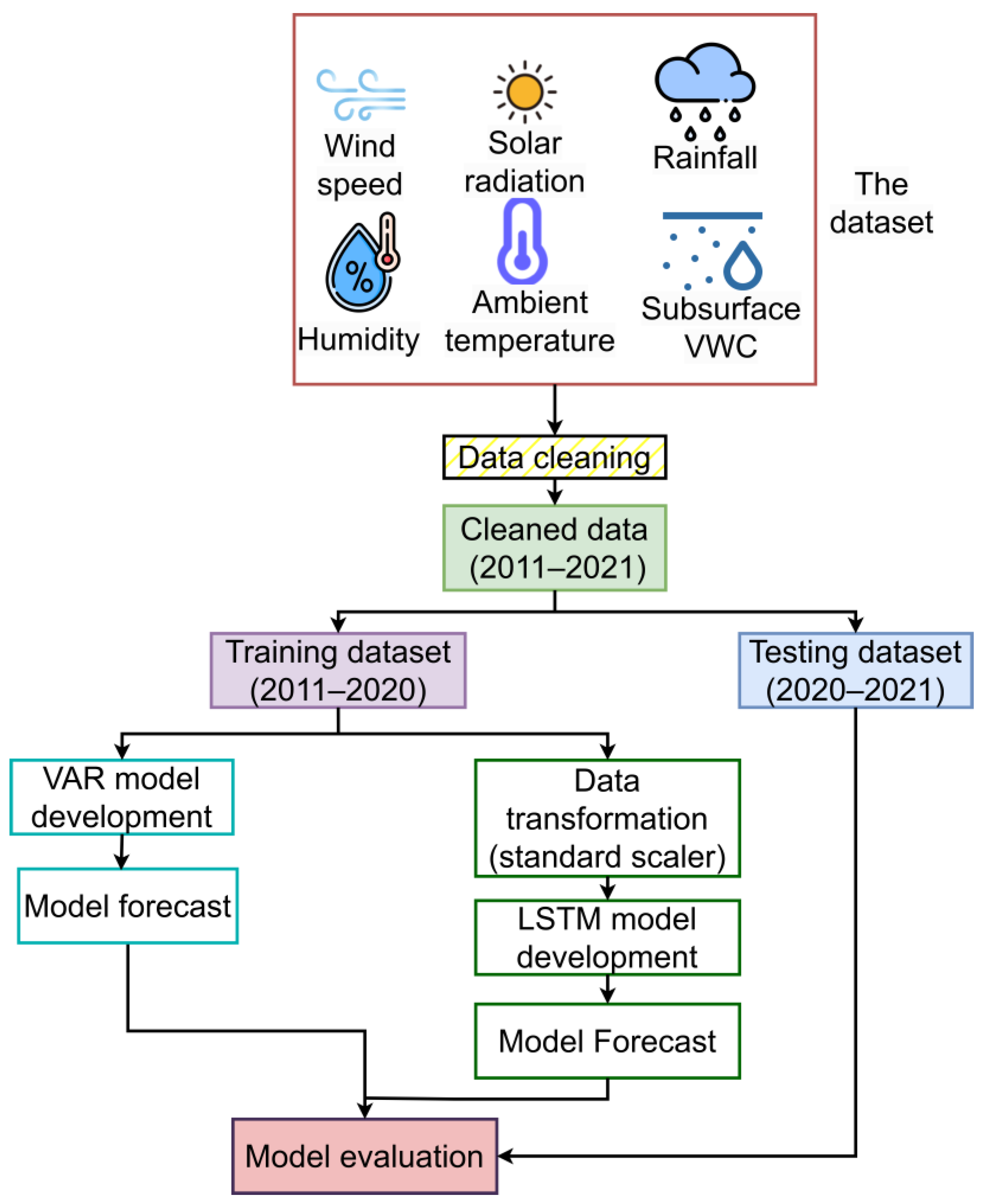
2. Materials and Methods

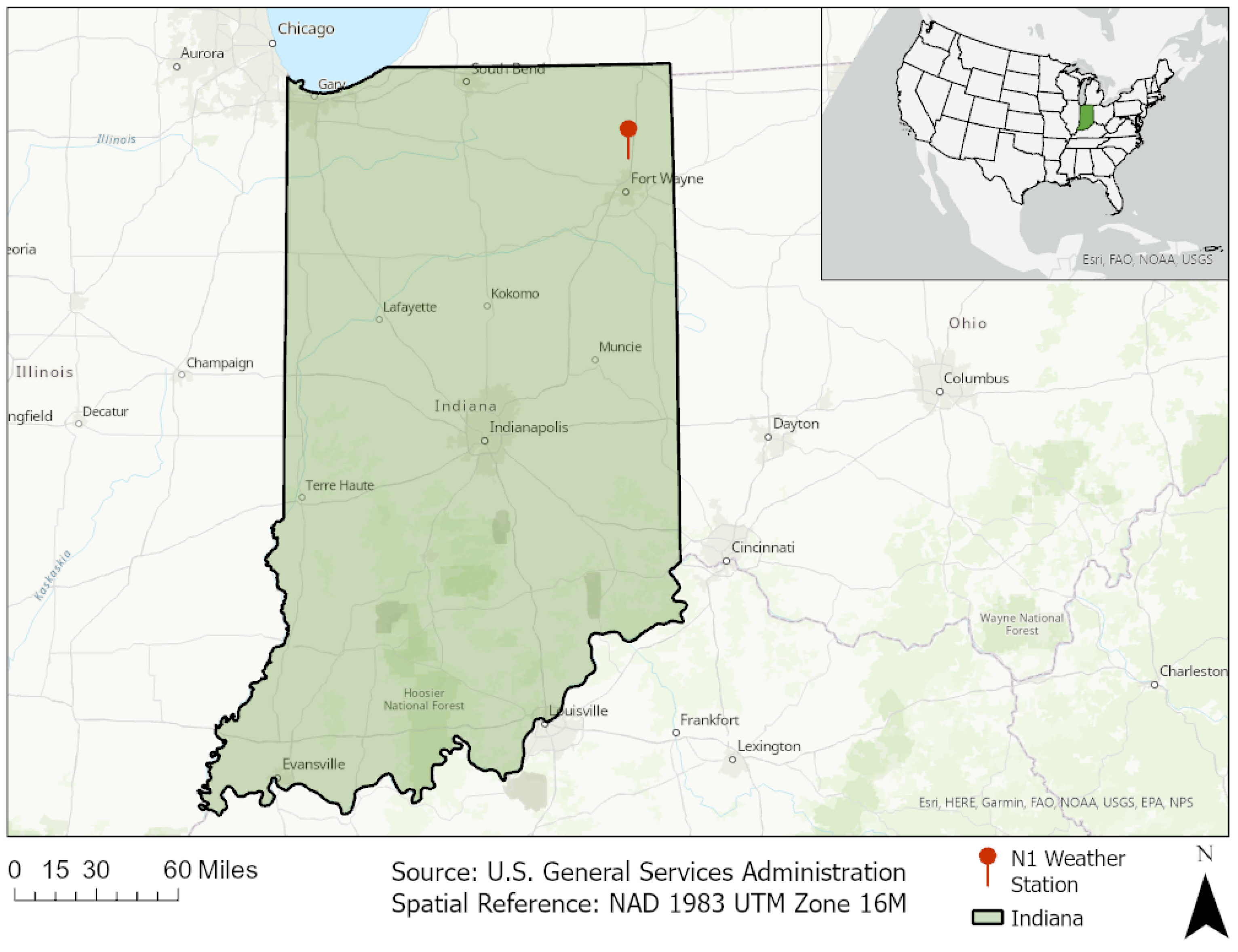
2.1. Study Area and Data Used

The dataset utilized in this research originates from a weather station located in Fort Wayne, Indiana, USA. The data span from 22 September 2011 to 9 September 2021, comprising a total of 87,362 samples. The selected data elements for this study include key meteorological variables such as ambient temperature (°C), relative humidity (%), solar radiation (Wm⁻²), wind speed (ms⁻¹), total rainfall (mm), and the volumetric water content (VWC) (m³m⁻³) of subsurface soil at a depth of 30 cm. The dataset was obtained from the Indiana Geological and Water Survey, Indiana University [37].

The dataset consists of daily records (daily average of hourly measurements) providing comprehensive insights into the temporal variation of these variables. There is a gap in the soil moisture time series data, specifically from 23 March 2015, 11:10 a.m., to 21 April 2015, 1:10 p.m., where the information is missing.

Figure 1 illustrates the geographical position of the study area, while

Table 1. Site description.

Specifications	Description
Latitude	41.2476079°
Longitude	−85.1182531°
Altitude	266.65 m
Soil parent	Glacial till
Vegetation	Conservation/Prairie
Landscape	End moraine
Slope	2–6%
Soil texture	Clay loam
Soil profile makeup	0–17.78 cm: silt loam
	Bulk density(g/cm3): 1.30–1.65
	Average sand, silt, clay (%): 22, 52, 26
	17.78–63.5 cm: clay
	Bulk density(g/cm3): 1.45–1.70
	Average sand, silt, clay (%): 22, 36, 42
	63.5–73.66 cm: clay loam
	Bulk density(g/cm3): 1.60–1.80
	Average sand, silt, clay (%): 24, 40, 36

presents a succinct overview of the soil conditions at the site, providing valuable context for this research.

The data were cleaned for model development after conducting time series forecastability and interdependency analysis by removing the missing data points (rows containing cells with no data or ‘NaN’) from the dataset.

2.2. Time Series Analysis

To develop forecasting models for a time series variable based on other time series variables, it is necessary to test their forecastability and examine the relationship between the dependent variable and the independent input variables (predictors). Subsurface soil water content was the dependent variable, which was subjected to forecasting depending on input variables, i.e., rainfall, air/ambient temperature, wind speed, relative humidity, and solar radiation. Due to the time series analysis result, the soil water content of the previous days was also considered as an input variable.

Some statistical tests were carried out to analyze the time series of variables to validate that the series is autocorrelated, stationary, cointegrated to soil moisture series, and interdependent.

Table 2. Statistical tests for time series analysis.

Subject to Test	Name of the Test	Python Library Tool Used
Autocorrelation	Durbin-Watson test [38,39]	statmodels-stattools
Stationarity	Augmented Dickey-Fuller test (ADF) [40]	statmodels-stattools
Cointegration Test	Johansen’s cointegration test [41]	statmodels-stattools
Interdependency of variables	Granger causality test [42,43]	statmodels-stattools
Seasonality test	Seasonal decompose (additive) [44]	statmodels-tsa-seasonal_decompose

shows the tests used for this purpose.

To be a pattern-following time series, variables need to be autocorrelated. The Durbin–Watson test shows whether the variables were autocorrelated or not [45]. Also, an additive seasonal decompose of soil moisture time series was conducted to check whether the trend of subsurface soil moisture increased or decreased throughout the recorded time and the seasonal pattern of soil moisture to support the forecastability of soil moisture. Both inputs and dependent variables need to be stationary to be forecasted, i.e., they do not depend on the observation time within the series [46,47]. Johansen’s cointegration test was conducted to evaluate the cointegration of the variables. This test refers to the relation between two or more time series variables. Another test for the interdependency of input variables and the target variable was determined by the Granger causality test. Seasonal decomposition was conducted to check if the moisture content data have any trend or seasonal changing pattern. It also gives insight into stationarity.

2.3. Model Development for Subsurface Soil Moisture Forecasting

Based on the results of the time series analysis, it was discerned that strong autocorrelation and cointegration exist within the subsurface soil moisture data. Consequently, a decision was made to employ two distinct algorithms: a statistical model, VAR [48], and a machine learning model, the LSTM network. VAR is recognized for its aptitude in managing cointegrated time series data, rendering it an appropriate choice for this particular context. Conversely, LSTM networks are distinguished for their proficiency in capturing intricate temporal patterns, thus enabling the effective utilization of multiple time series inputs for enhanced predictive capabilities. The steps of developing the models are briefly described in Figure 2. The dataset of historical weather and VWC was cleaned, the missing data rows were deleted, and the dataset was split into two parts: training and testing. The models were developed using the training dataset, and their forecasting performance was evaluated using the testing dataset.

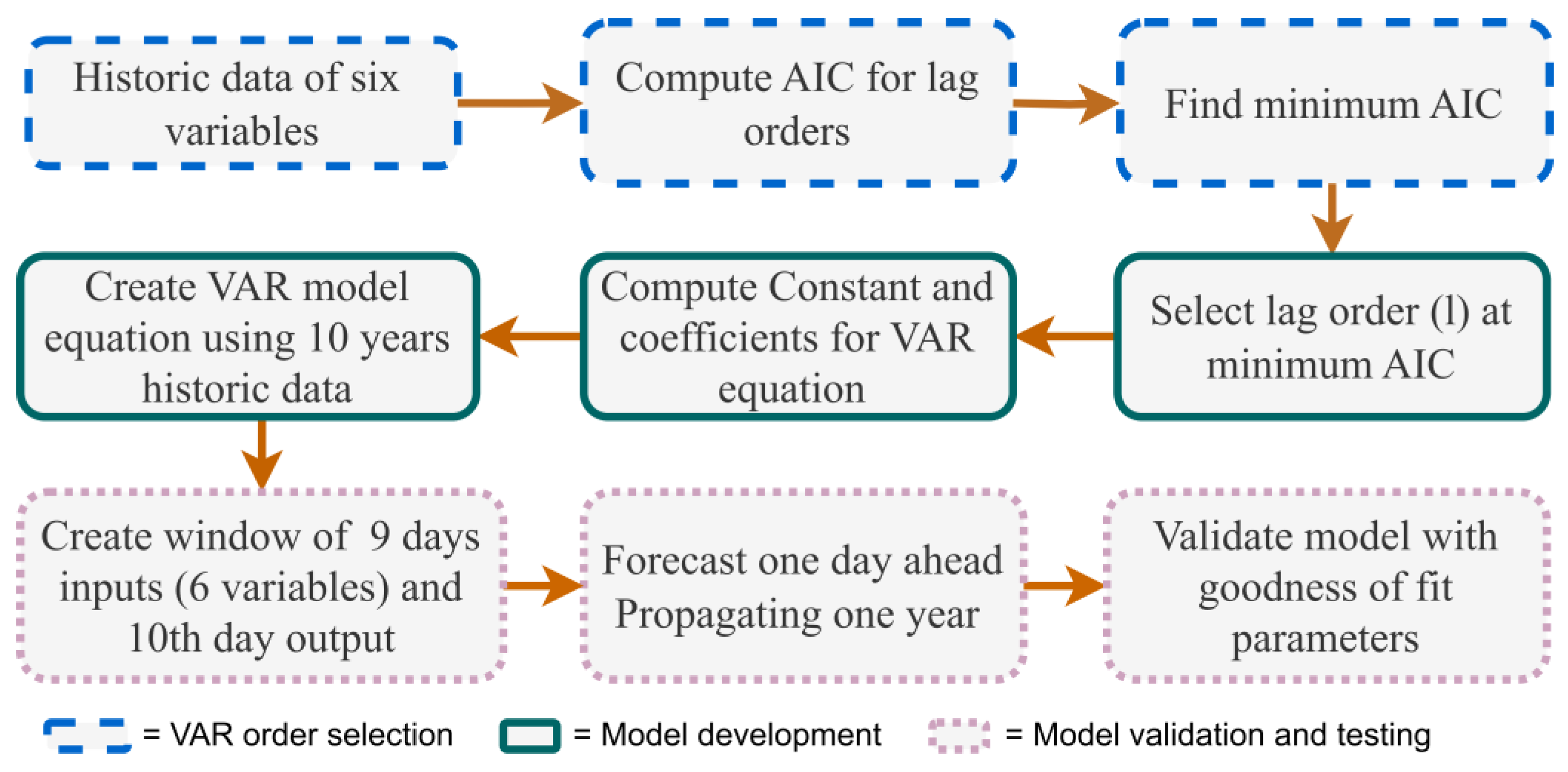
2.4. Development of a VAR Model

The VAR model requires the temporal input and output data to be stationary and autocorrelated. The method of testing stationarity, autocorrelation, and forecastability was described and demonstrated in the previous section, and depending on the statistical test results, a multivariate time series forecasting model was attempted to develop using the VAR [48] algorithm. Three steps were followed to develop a VAR model to forecast the subsurface soil moisture. The determination of the order of VAR using AIC (Akaike Information Criteria) [49], Running the VAR algorithm with selected order to train the VAR model with 10 years of historical weather and subsurface soil moisture data and validation of the model by forecasting one day throughout the next one year. The model was developed using the ‘Statmodels’ tool in Python language. Figure 3 briefly describes the development stages of the VAR model.

2.4.1. Selection of Lag Order

The selection of the lag order or length for the VAR model was conducted by assessing the AIC (Akaike Information Criteria) value [49,50,51,52]. The computed AIC values are provided in

Table 3. Selection of order of Vector Auto Regression (* represents the minimum).

Lag Order	AIC
0	7.956
1	−0.7902
2	−1.114
3	−1.202
4	−1.238
5	−1.269
6	−1.297
7	−1.31
8	−1.31
9	−1.314 *
10	−1.314
11	−1.306
12	−1.3
13	−1.293
14	−1.283

.

As the AIC value shows a minimum at the 9th lag, so 9 was selected as the order of VAR.

2.4.2. Construction of Model Equation

The VAR model was built using the selected lag order 9. The equation (Equation (1)) developed for the VAR model using 9 as lag is as follows [53]:

$${\mathrm{Y}}_{\mathrm{t}}={\mathrm{A}}_0+{\sum }_{\mathrm{l}=1}^9{\sum }_{\mathrm{v}=1}^6{\mathrm{A}}_{\mathrm{v},\mathrm{l}}{\mathrm{Y}}_{\mathrm{t}-\mathrm{l}}+{\mathrm{e}}_{\mathrm{t}}$$

(1)

where ${\mathrm{Y}}_{\mathrm{t}}$ = output vector at time t (here subsurface moisture content), ${\mathrm{A}}_0$ = a constant value (vector intercept), ${\mathrm{A}}_{\mathrm{v},\mathrm{l}}$ = coefficient matrix for each variable and lag combination, ${\mathrm{Y}}_{\left(\mathrm{t}-\mathrm{l}\right)}$ = vector of exogenous variables, ${\mathrm{e}}_{\mathrm{t}}$ = residual vector at time t.

2.4.3. VAR Model Evaluation

The VAR model was trained with historical weather data and subsurface soil water data from 2011 to 2020. The model accuracy was tested using the following year’s forecasts of corn cropping season data (March–September 2021). The evaluation was performed by measuring the mean squared error (MSE) [54], mean absolute error (MAE), and root mean squared error (RMSE) [55]. The goodness-of-fit parameter (R²) was also calculated. The Durbin–Watson test for the residuals was conducted to check if there was any autocorrelation among the residuals.

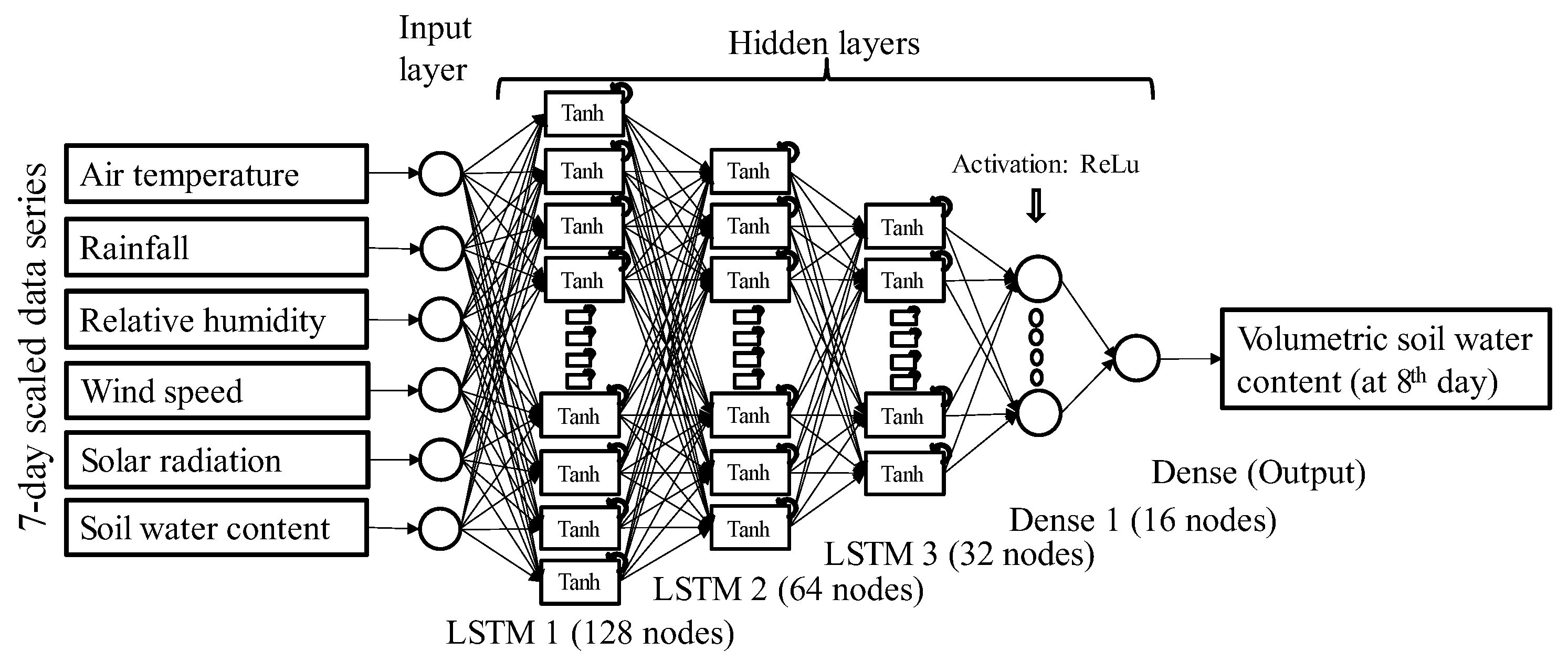
2.5. Development of an LSTM Model

A simple LSTM network model was also developed for the purpose of forecasting subsurface soil moisture. This model leverages input variables, including rainfall, air temperature, relative humidity, solar radiation, wind speed, and the historical soil water content data from the preceding n days. The normalized (min–max scaled) training dataset encompasses a daily record spanning nine years (22 September 2011 to 10 September 2019) and tested with the following two years (11 September 2019 to 9 September 2021) daily basis data.

2.5.1. Architecture of the LSTM Model

The LSTM network model was implemented using the Python programming language within the Jupiter Notebook environment of the Anaconda Navigator Software (Anaconda3, developer: Continuum Analytics). This model was designed to accommodate six input variables, resulting in an input layer with six neurons. The output layer was configured with a single neuron, as the sole objective was to forecast subsurface soil water content. The model architecture incorporated five hidden layers and employed the ‘Adam’ optimizer [56] to estimate the error or loss for training and optimization purposes, which were set by trial and error according to the model’s best fit. A succinct overview of the model’s structure is presented in

Table 4. Structure of the LSTM network model.

Layer (Type)	Nodes	Parameter	Activation Function
LSTM [1]	128	69,120	Tanh
LSTM [2]	64	49,408	Tanh
LSTM [3]	32	12,416	Tanh
Dense	16	528	ReLU *
Dense (output)	1	33	Linear

* ReLU: Rectified Linear Unit.

.

In this model, three LSTM layers and two dense layers were used. LSTM layers forward the trend of data and the LSTM cell value to the next layer, and the dense layer forwards the dense output of the dense layer to the next layer [57]. The three LSTM layers used a tanh activation function that scales the output of those layers between −1 and 1, where ReLU makes the output maximized and passes only the positive values to the next layer [58,59,60]. The output layer was given a linear activation so that it may pass the dense output as it was generated. The architecture of the developed LSTM model is shown in Figure 4.

2.5.2. Training the LSTM Model

The model was trained to attain minimal training and validation losses, with their estimation being refined through a systematic trial-and-error approach. The Mean Absolute Error (MAE) served as the loss function and was optimized to minimize deviations. Additionally, trial-and-error was conducted to estimate the optimal number of hidden layers, aiming to identify the configuration that yielded the lowest loss values.

The constructed LSTM network model was trained using 2883 inputs from a ground truth dataset of subsurface soil water content and weather variables, where 20% of the series data was used for validation. The training and validation set was split into blocks containing n rows of data as a single input and the following one of soil water content as output. The sliding window algorithm was used to make the batch input for training the model so that the model should be able to forecast the soil moisture of the (n + 1)th day as an output of feeding the previous n days’ input data. The model was optimized by minimizing validation errors. The model training and validation phase were programmed to iterate over 90 epochs, aiming to identify the most appropriate parameter combination that resulted in minimal training and validation errors while achieving optimal accuracy.

2.5.3. Overfitting and Underfitting Test of LSTM Model

The LSTM model involves a trial-and-error process to determine optimal hyperparameters and the number of hidden layers, which can lead to overfitting or underfitting issues. Underfitting occurs when the model inadequately fits the training data, resulting in poor performance during validation; this is typically indicated by a much lower validation R² value compared to the training R². Conversely, achieving high R² values in both training and validation does not guarantee a well-fitted model, as there could be overfitting, wherein the model excessively memorizes the training data. In these instances, the model lacks the ability to generalize. Overfitting can arise due to model complexity, including unnecessary hidden layers. To combat overfitting and underfitting in the developed LSTM model, an early stopping callback function was utilized during LSTM training to halt the process at the optimal epoch. Furthermore, in assessing overfitting and underfitting, two parameters were measured: Cost Delta (the difference between training and validation MAE) and the Overfitting Ratio (OR) [61]:

OR = (Validation R²/Training R²)

(2)

The model was optimized to obtain a minimum cost delta, ensuring minimal training and validation loss. An Overfitting Ratio (OR) close to 1 indicates balanced model performance—achieving a level of equilibrium between the model’s fitting to the training data and its generalization to unseen data [62].

2.5.4. Testing the LSTM Model

The model’s performance was evaluated by comparing its anticipated subsurface soil moisture values with actual data from a separate validation dataset that had not been employed during the training and validation phases. The testing was performed using two years of data, including the cropping season of corn (1 March 2020 to 25 October 2020 and 2 March 2021 to 9 September 2021).

The model’s performance was assessed by employing statistical error measures that quantify the disparities between anticipated and actual values. Statistical goodness-of-fit measures and error parameters such as the coefficient of determination (R²) [63], Mean Squared Error (MSE) [54], Root Mean Squared Error (RMSE) [55], and Overall Performance Index (OI) [64] were determined to evaluate the forecasting accuracy. A residual analysis of the normality of residual distribution and assumption of ‘zero’ mean of error was tested to evaluate the suitability of the constructed model.

3. Results and Discussions

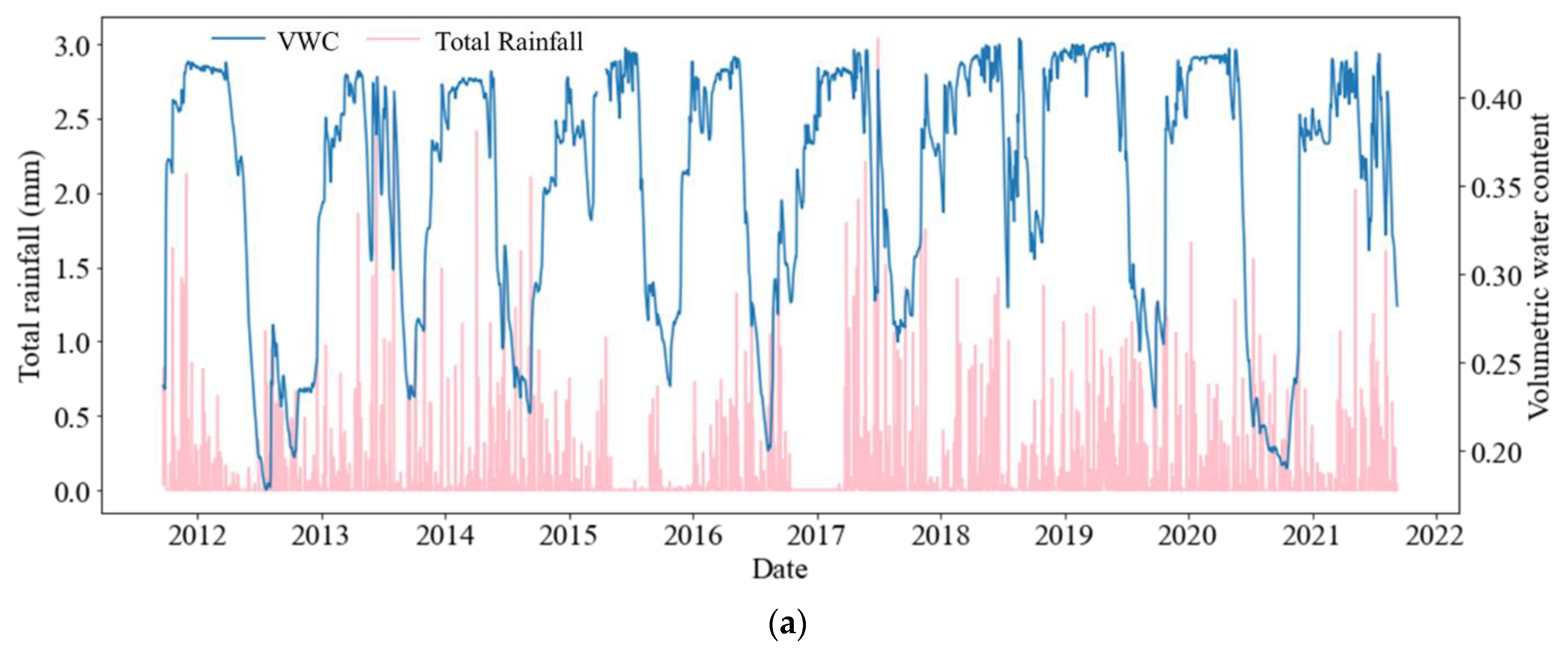
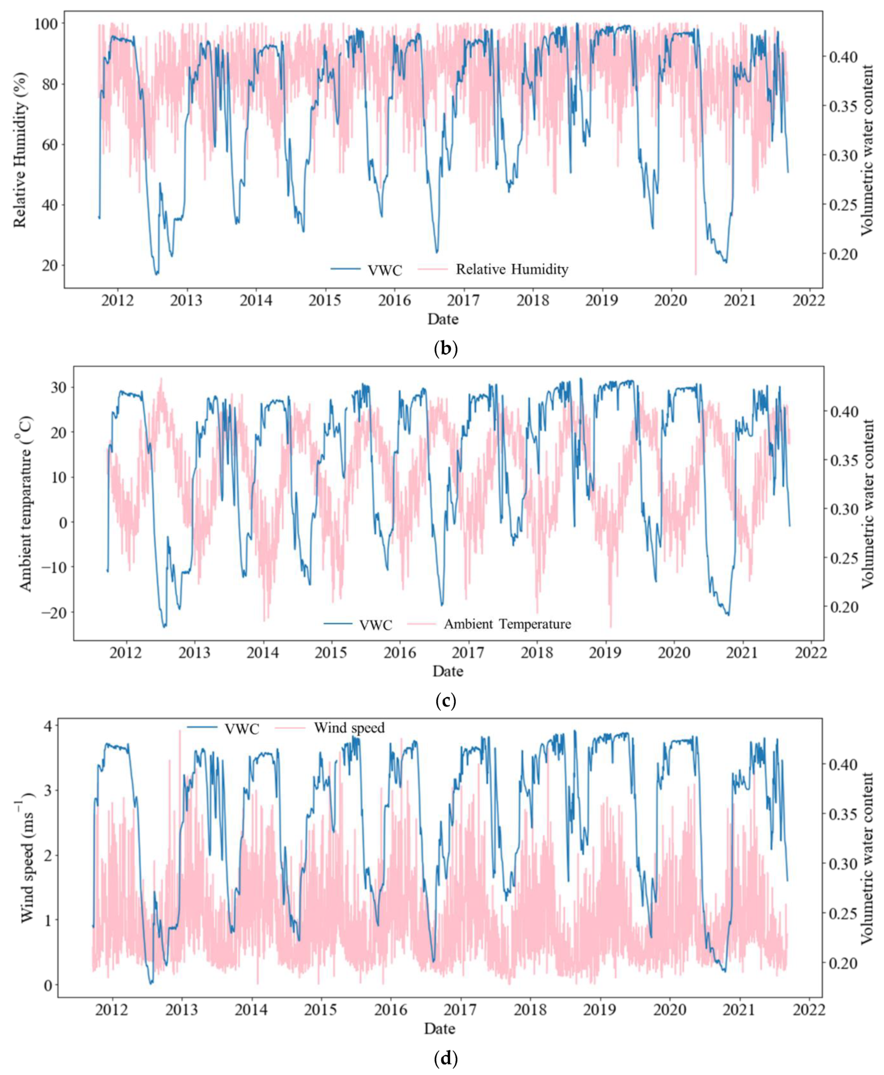
3.1. Subsurface Soil Water Content in Response to Weather Variables

Figure 5 illustrates the relationship between VWC and the weather variables over time. These variables consistently exhibit discernible patterns that demonstrate a temporal correlation with subsurface soil moisture. These weather variables have individual effects on the rate of change in soil moisture based on physics; they also are interrelated due to seasonal patterns (i.e., their time series cross-correlation [65]). Rainfall has an obvious positive effect on subsurface soil water content. The soil water content directly increases with additional rainfall. In the case of relative humidity, it shows a slightly different scenario. Following the peak values of relative humidity, the change in soil moisture is noticed a few days later. When ambient temperature increases, soil moisture decreases (evapotranspiration) with a lag of a few days. Wind effect on soil moisture also depends on temperature and solar radiation. They are positively correlated, yet the graph shows a positive relation between wind speed and subsurface soil moisture. Solar radiation has a direct opposite relationship with soil moisture, albeit delayed, as seen in the figure. So, the variables are not instantaneously correlated, but soil moisture is related to the history of those variables. As expected, there is a seasonal pattern (cycle) in the time series of weather variables.

3.2. Time Series Analysis of the Variables

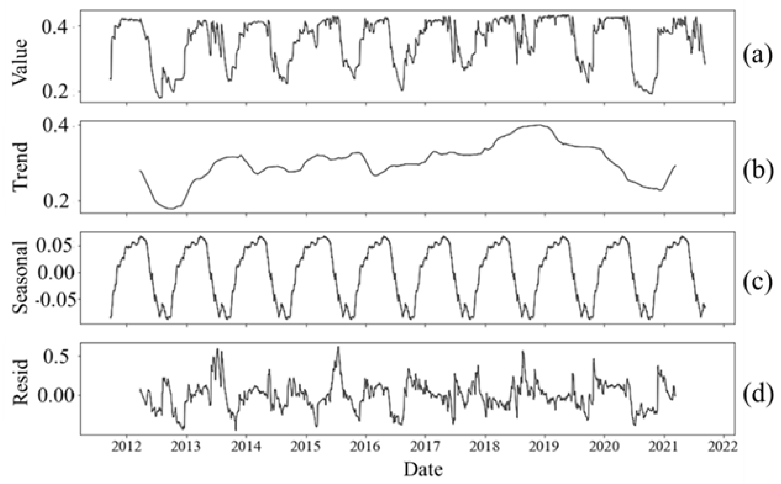
3.2.1. Analysis of Historical Subsurface Soil Moisture Data

The subsurface soil moisture data from 2011 to 2021 shows an average moisture content of 35.3%. Figure 6 depicts the distribution of subsurface soil moisture in months of a year. In the months of December to May, the subsurface soil moisture is higher than the average. It decreases from April to September due to warmer temperatures, lower rainfall, and moisture uptake due to vegetation during this part of the year. The soil moisture increases from October to April because of precipitation and low temperatures.

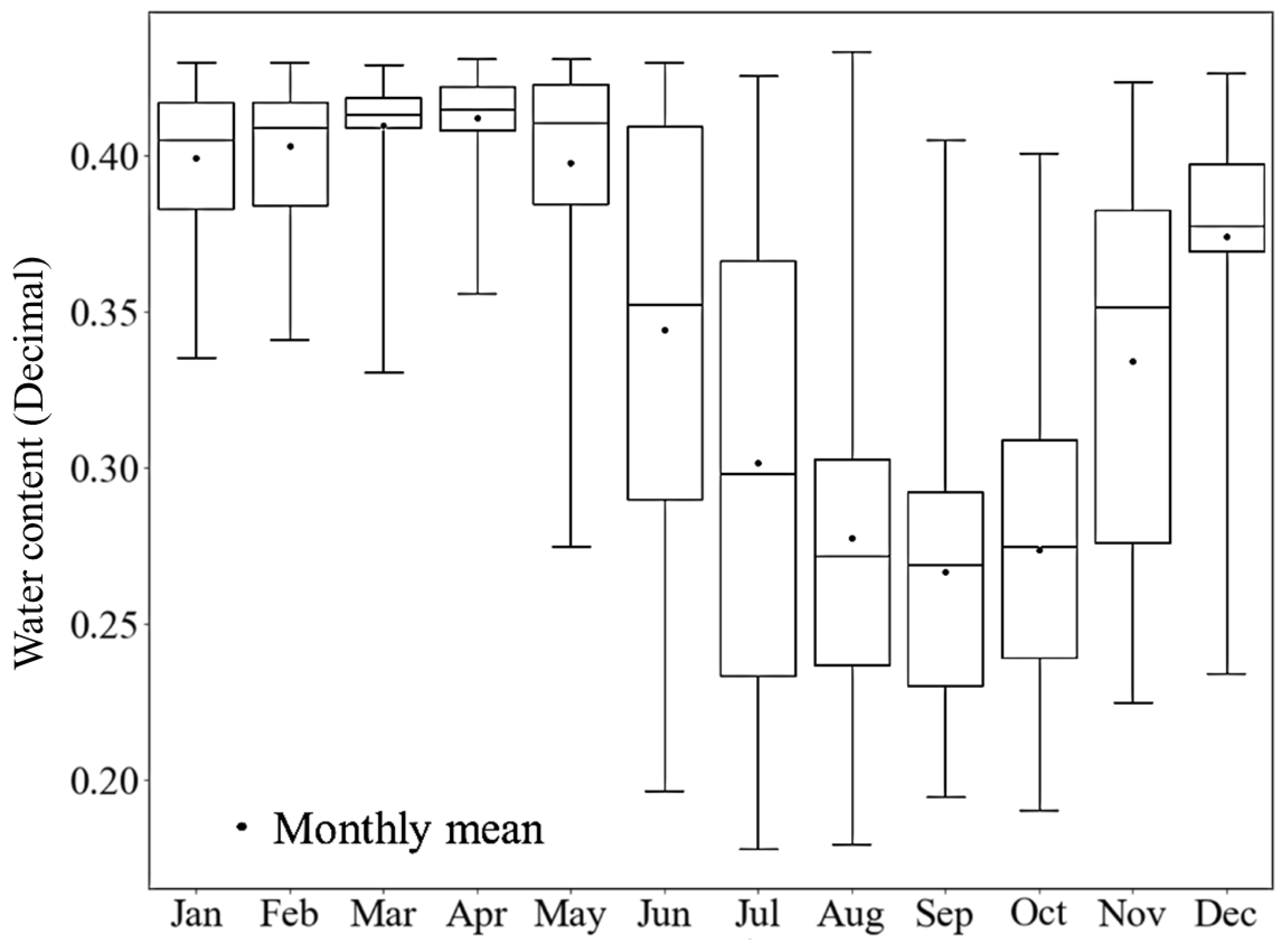
3.2.2. Seasonality of Moisture Content

The seasonal decomposition illustrated in Figure 7 demonstrates that there is a consistency among yearly cycles in the subsurface soil moisture level (seasonality, Figure 7b). This result verifies the result shown in Figure 5 that there are seasonal patterns in subsurface soil water content. Since there is no trend throughout the recorded time (across seasons), the data are stationary (Figure 7c).

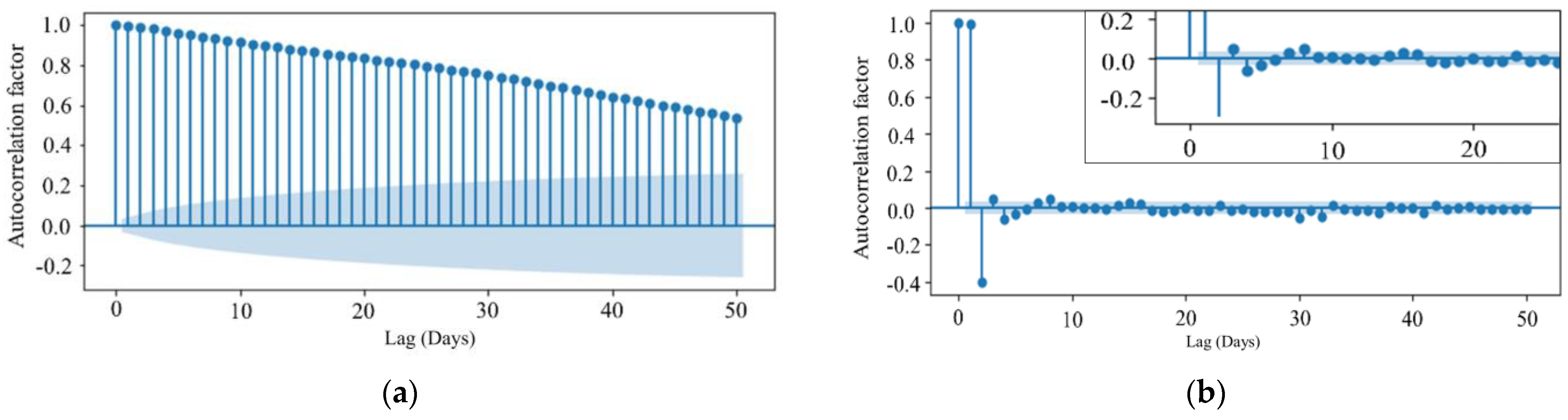
3.2.3. Autocorrelation Test of Variables

Figure 8 shows the autocorrelation in subsurface soil moisture data. Figure 8a shows that as the autocorrelation factor decreases rapidly, the dataset comprises non-random and stationary data. Also, it depicts that the soil moisture of previous days ((n − l)th days) is positively correlated to the present value (nth day). The partial autocorrelation plot (Figure 8b) shows the significance of correlations of lags with the first lag [66]. Here, the partial autocorrelation factor is significant for the 1st and second lag (near 1), and correlation remains significant (outside the shaded area of confidence) through the 6th lag (days) (Figure 8b). It shows a pattern where the subsequent lags exhibit a positive-negative-positive sequence in the partial autocorrelation. This pattern implies a cyclical or oscillatory behavior in the relationship between the variable and its past values, possibly indicating a recurring pattern or seasonality in the soil moisture data, which validates Figure 7.

The Durbin–Watson test gives an interpretation of existing autocorrelation inside the time series variables. This test also establishes a series as an autocorrelated time series.

Table 5. Durbin –Watson test for autocorrelation.

Variables	Durbin Watson Statistics
Total rainfall (mm)	1.545
Air temperature (°C)	0.057
Relative humidity (%)	0.012
Wind speed (ms−1)	0.319
Solar radiation (Wm−2)	0.179
Subsurface water content (m3m−3)	0.0003

shows the Durbin–Watson test for detecting autocorrelation.

The Durbin–Watson statistics near 2 indicate no autocorrelation. The possible values of Durbin–Watson statistics range from 0 to 4. Statistics test results of less than 2 indicate positive correlation, and greater than 2 indicate negative autocorrelation [39,67]. The test result shown in Table 5 shows that variables are positively correlated.

3.2.4. Stationarity Test

The Augmented Dicky–Fuller (ADF) test is statistical evidence of stationarity. The ADF test result for all considered variables (inputs and target) is shown in

Table 6. Augmented Dickey–Fuller test result for stationarity checks on soil volumetric water content.

Variables	ADF Statistics	p-Value	Critical Values
			1%	5%	10%
Total Rainfall (mm)	−24.382	2.00 × 10−6	−3.432	−2.862	−2.567
Air temperature (°C)	−3.251	1.72 × 10−2	−3.432	−2.862	−2.567
Relative humidity (%)	−5.339	5.00 × 10−6	−3.432	−2.862	−2.567
Wind Speed (ms−1)	−4.479	2.14 × 10−4	−3.432	−2.862	−2.567
Solar radiation (Wm−2)	−3.678	4.44 × 10−3	−3.432	−2.862	−2.567
Water content (m3m−3)	−4.384	3.17 × 10−4	−3.432	−2.862	−2.567

.

ADF statistics for all the variables are negative. The more negative the ADF statistics, the more the variables are likely to be stationary. ADF statistics value less than the critical value for a certain confidence interval (1%, 5%, or 10%) refers to a stationary pattern of data [40]. Here, the ADF statistics value for all the variables except the air temperature is less than the critical value at a 1% confidence interval. The air temperature shows ADF statistics less than the critical value at a 5% confidence interval. Still, all the variables are significantly stationary. The p-values displayed in the table also prove the time series of each variable as stationary. The p-values are less than 0.01 for all the variables and less than 0.05 for air temperature.

3.2.5. Cointegration Test

Johansen’s cointegration test gives the scenario if three or more time series are related to each other. The test result aimed to determine the statistical relationship between subsurface soil water content and the input weather variables is presented in

Table 7. Summary of Johansen’s cointegration test (cointegration with water content).

Variables	Test Stat	Critical Value at 95% Confidence Level
Total Rainfall (mm)	1104	83.9
Air temperature (°C)	607	60.0
Relative humidity (%)	266	40.1
Wind Speed (ms−1)	120	24.2
Solar radiation (Wm−2)	33	12.3

.

Johansen’s cointegration test shows that the test statistics for the input variables are larger than the critical value at a 95% confidence level. So, it is an indicator for the variables to be cointegrated with soil water content [42,68].

3.2.6. Forecastability Test

The Granger causality test shown in

Table 8. Result of Granger causality test (p-values).

Variables	Total Rainfall (mm)	Air Temperature (°C)	Relative Humidity (%)	Wind Speed (ms−1)	Solar Radiation (Wm−2)	Water Content
Total Rainfall (mm)	1.0	<0.0001	<0.0001	<0.0001	<0.0001	0.0002
Air temperature (°C)	<0.0001	1.0	<0.0001	<0.0001	<0.0001	<0.0001
Relative humidity (%)	<0.0001	<0.0001	1.0	<0.0001	0.0108	0.0004
Wind Speed (ms−1)	<0.0001	<0.0001	<0.0001	1.0	<0.0001	<0.0001
Solar radiation (Wm−2)	<0.0001	<0.0001	<0.0001	<0.0001	1.0000	<0.0001
Water content (m3m−3)	<0.0001	<0.0001	<0.0001	<0.0001	<0.0001	1.0000

demonstrates that all the input variables may be useful in forecasting subsurface soil water content. It verifies the forecastability of time series in water content with weather inputs. The p-values below 0.01 indicate that the time series of water content is significantly dependent on the time series of weather inputs (data concerning moisture content depends on the past data concerning weather time series) [69].

The statistical tests and analysis show that the subsurface soil moisture can be defined by the weather conditions, and it can be forecasted from historical weather data and previous data on subsurface soil moisture content.

3.3. Model Development and Evaluation of Subsurface VWC Forecast

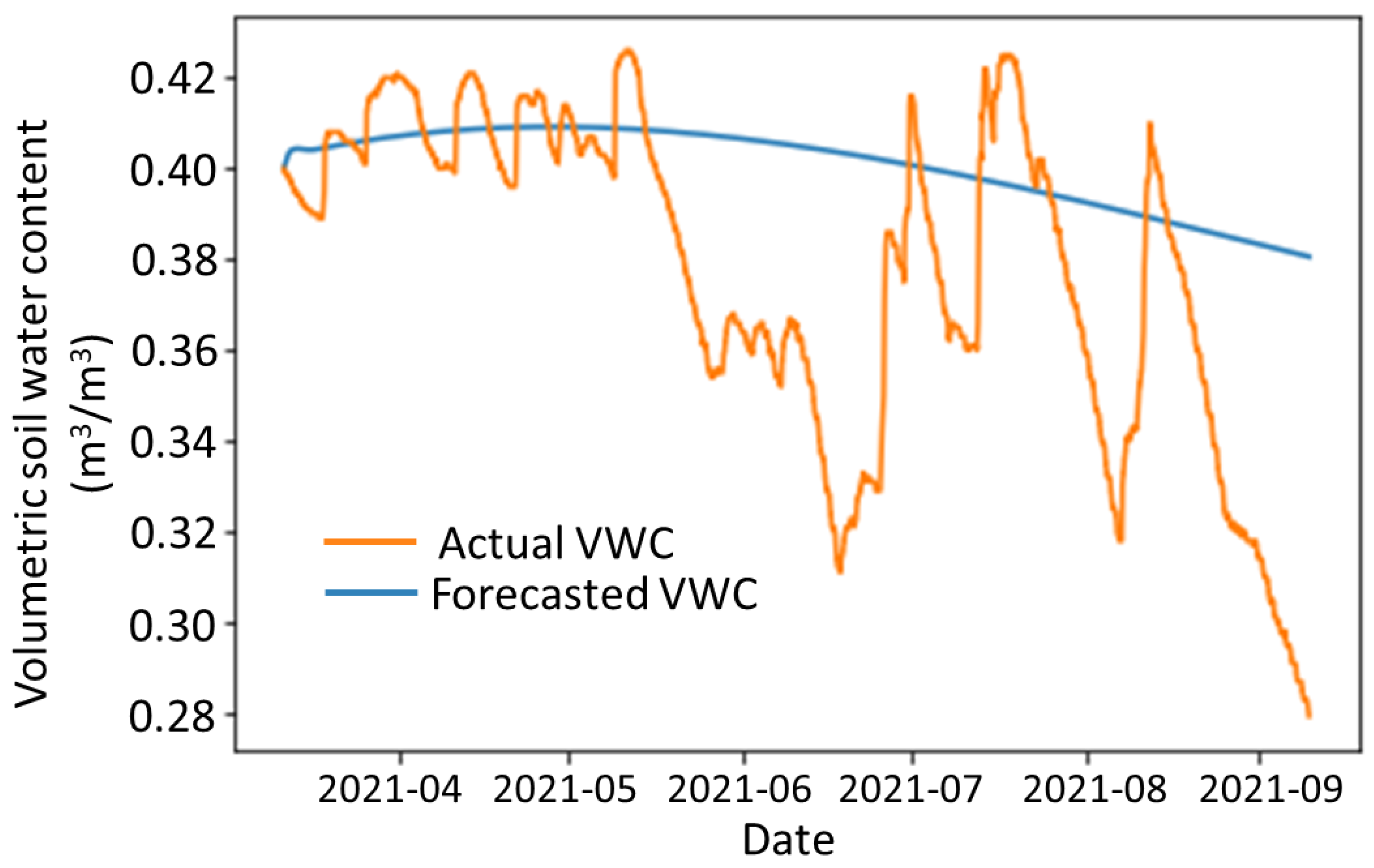
3.3.1. Statistical Model: Vector Autoregression (VAR)

The VAR model (Equation (1)) constant and coefficients (A₀ and A_n) for all the input variables are shown in

Table 9. Constant and coefficients for Vector Autoregression model equation.

Constant, A0 = 0.002924
Coefficients (An)
Lag Order	Rainfall (A1) (mm)	Air Temperature (A2) (°C)	Relative Humidity (A3) (%)	Wind Speed (A4) (ms−1)	Solar Radiation (A5) (Wm−2)	Water Content (A6) (m3m−3)
L1	8.100 × 10−3	1.200 × 10−4	1.700 × 10−5	−2.900 × 10−4	−1.000 × 10−5	1.295 × 100
L2	−2.340 × 10−3	−1.000 × 10−5	1.900 × 10−5	3.900 × 10−4	2.100 × 10−6	−3.150 × 10−1
L3	2.600 × 10−4	−3.100 × 10−5	−2.100 × 10−5	−8.900 × 10−5	−1.700 × 10−6	3.920 × 10−2
L4	6.200 × 10−4	2.800 × 10−5	1.300 × 10−5	2.800 × 10−4	0.000	−1.690 × 10−2
L5	−2.100 × 10−4	−7.900 × 10−5	8.800 × 10−6	5.400 × 10−4	−1.300 × 10−6	−1.100 × 10−3
L6	−1.400 × 10−4	−1.900 × 10−6	−3.500 × 10−5	−2.700 × 10−4	−1.100 × 10−6	−2.130 × 10−2
L7	2.700 × 10−4	−1.500 × 10−5	1.900 × 10−5	−2.000 × 10−4	0.000	1.600 × 10−2
L8	−4.300 × 10−4	3.600 × 10−5	−1.500 × 10−5	1.100 × 10−4	1.200 × 10−6	3.000 × 10−3
L9	−5.400 × 10−4	−7.800 × 10−5	1.200 × 10−5	−1.300 × 10−5	1.900 × 10−6	−1.120 × 10−2

.

Following Table 9, to forecast the subsurface water content at time t from weather and water content inputs, Equation (3) can be formed.

$${(\mathrm{V}\mathrm{W}\mathrm{C})}_{\mathrm{t}}={\mathrm{A}}_0+{\sum }_{\mathrm{l}=1}^9\left({\mathrm{A}}_{1,\mathrm{l}}\right){\left(\mathrm{RF}\right)}_{\mathrm{t}-\mathrm{l}}+({\mathrm{A}}_{2,\mathrm{l}}\left){\left(\mathrm{AT}\right)}_{\mathrm{t}-\mathrm{l}}+({\mathrm{A}}_{3,\mathrm{l}}\right){\left(\mathrm{RH}\right)}_{\mathrm{t}-\mathrm{l}}+({\mathrm{A}}_{4,\mathrm{l}}){\left(\mathrm{WS}\right)}_{\mathrm{t}-\mathrm{l}}+({\mathrm{A}}_{5,\mathrm{l}}\left)\right({\mathrm{SR})}_{\mathrm{t}-\mathrm{l}}+({\mathrm{A}}_{6,\mathrm{l}}\left)\right({\mathrm{V}\mathrm{W}\mathrm{C})}_{\mathrm{t}-\mathrm{l}}$$

(3)

where VWC = volumetric subsurface water content (m³m⁻³), Rf = rainfall (mm), AT = air temperature (°C), RH = relative humidity (%), WS = wind speed (ms⁻¹), SR = solar radiation (Wm⁻²), l = lag number (1–9).

3.3.2. Evaluation of the VAR Model

The VAR model was evaluated by forecasting the subsurface moisture content of the following one-year (2020–2021) corn cropping season. Figure 9 shows the forecasted and recorded values of subsurface soil water content from 15 March 2021 to 9 September 2021. The model evaluation parameters are shown in

Table 10. Vector Autoregression Model performance of soil volumetric water content (m³m⁻³) evaluation.

Parameters	Values
MAE (m3m−3)	0.0561
MSE (m3m−3)2	0.0046
RMSE (m3m−3)	0.03821
R2	0.698
Durbin-Watson statistics	2.00

.

Despite error values (MAE, MSE, and RMSE) being small numerically and 69.8% of the variation being explained, VAR does not capture day-to-day variations (Figure 9). A t-test shows that the forecasted values of soil moisture were significantly different from the actual (p < 0.05).

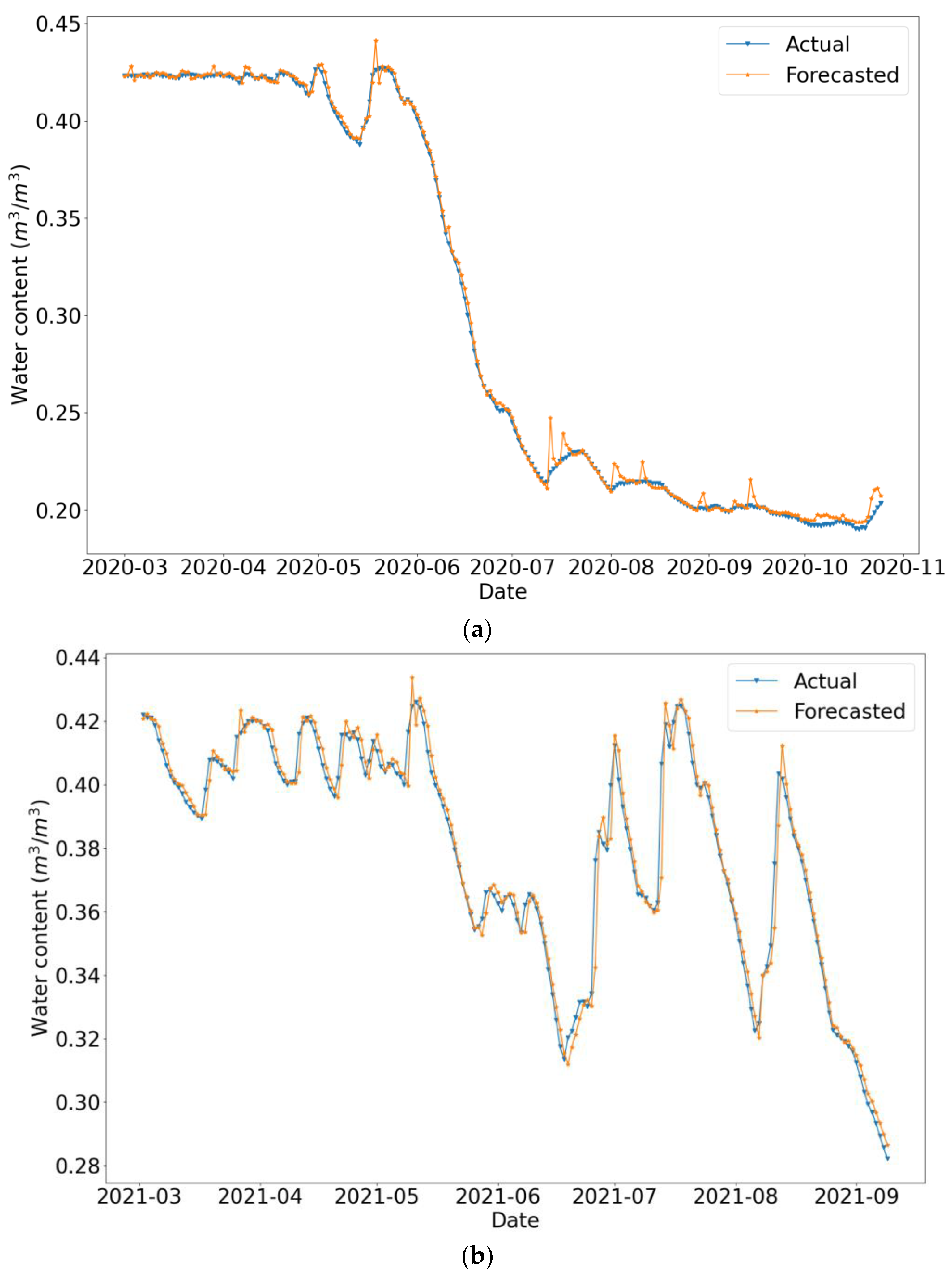
3.3.3. The LSTM Network Model

The LSTM model was trained using the training dataset with an n = 7 days sliding window, and the eighth-day soil moisture was forecasted. The model was iterated for a total of 90 epochs, and the highest accuracy while simultaneously minimizing training and validation errors was achieved during the 51st iteration. The iteration process ended once the training loss reached a minimum of 3.12%, and the validation loss matched at 1.29%. The model’s statistical metrics from the 51st epoch are detailed in

Table 11. Statistics of the developed Artificial Neural Network model for soil volumetric water content (m³m⁻³, after 51st Epoch).

Parameters	Training	Validation
Mean absolute error (m3m−3)	0.0093	0.0098
Mean absolute percentage error (MAPE)	3.12%	1.29%
Mean squared error (m3m−3)2	0.00031	0.00041
R squared	0.995	0.981
Cost delta (m3m−3)	0.0005 (5.37% of training MAE)
Overfitting ratio (OR) [61]	0.93

.

Figure 10 portrays the loss minimization process for the entire model over the course of 51 epochs. The graph illustrates the declining trend of both training and validation losses, measured in terms of Mean Absolute Error (MAE), with each successive epoch. From Table 11, the high accuracy of the model at the 51st epoch is evidence of no underfitting. The cost delta, representing a 5.37% difference between validation and training errors, indicates a minimal divergence, thus suggesting the absence of overfitting. Typically, overfitting would lead to poor validation results. In this scenario, the validation R² (0.981) closely approximates the training R² (0.995), with an OR of 0.93, which indicates the model is balanced. The OR value exceeding unity is evidence of overfitting [62]. In Figure 10, it is shown that the training and validation loss moves downward in the 51st epoch, and their difference also decreases at that point, and the fluctuation is lower. However, as the graph shows a little noise in the training and validation loss curve in the last six epochs, there can be a chance of being slightly overfitted [70], which was tested later in the model evaluation section.

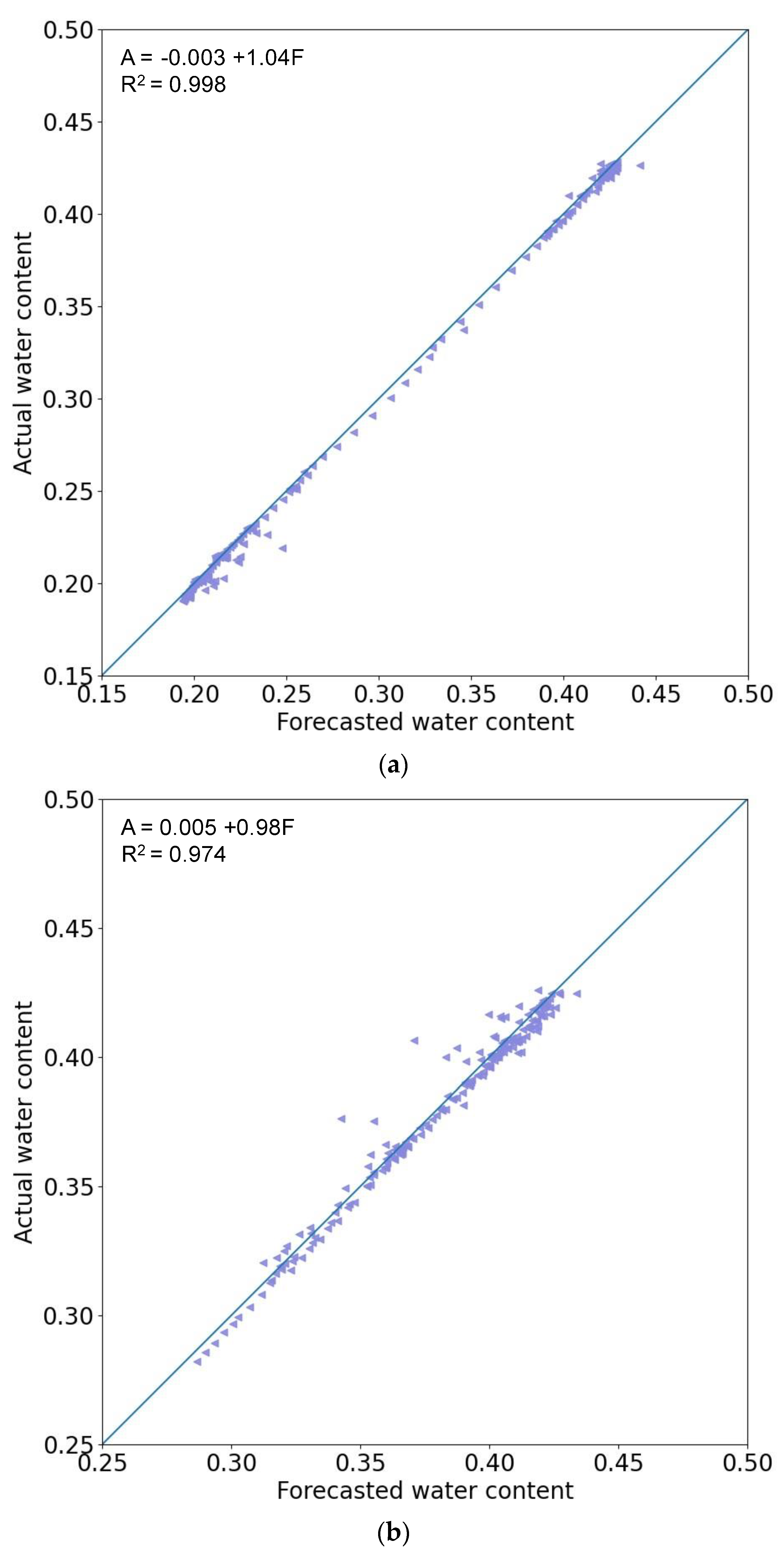
3.3.4. Evaluation of the LSTM Network Model

Figure 11 shows the forecasting accuracy of the LSTM network model for the corn-growing seasons of 2020 (Figure 11a) and 2021 (Figure 11b). The forecasts sometimes overshoot VWC; curves of actual VWC are smoother than forecasts, but overall, the difference between actual and forecasted moisture content was small (MAPE = 0.91%, p > 0.05 for the 2020 crop season and MAPE = 0.97%, p > 0.05 for the 2021 crop season).

Figure 12 shows the model fit for the testing series. In both cases, the intercept is not different from 0.0 (p < 0.001), and the slope is not different from 1.0 (p < 0.001). The goodness of model fit is also described in values in

Table 12. Goodness-of-fit for LSTM network model to soil moisture content (m³m⁻³).

Parameters	Test for Corn Cropping Season 2020	Test for Corn Cropping Season 2021
R2	0.998	0.973
Mean absolute error (MAE) (m3m−3)	0.00237	0.00368
Mean squared error (MSE) (m3m−3)2	0.000015	0.000033
Root mean squared error (RMSE) (m3m−3)	0.00382	0.00577
Overall performance index (OI)	0.992	0.966

.

Figure 12 shows that the LSTM forecasts of soil moisture average slightly lower than the actual value. The model fit is R² = 0.998 and R² = 0.973 (Table 12) for the cropping seasons of 2020 and 2021, respectively. The combination of low MSE and RMSE, along with a high R-squared (R²) value, indicates that this model can be an effective alternative to traditional empirical equations for soil moisture forecasting [71]. The acceptable threshold for RMSE value is 10% [72], where the model forecasted soil moisture with RMSE of 0.3% and 0.5% for two consecutive years. The overall performance index of the model also shows a satisfactory result with OI = 0.992 and 0.966. As the model test result shows a good performance in terms of goodness-of-fit parameters, it can be said that the overfitting issue is negligible.

Figure 13 shows the residual distribution of the forecasted series. The distribution curve shows a little skew in the error distribution. Also, the maximum density of errors gathers near zero, with the mean of error being −0.001 and −0.0006 for the cropping seasons of 2020 and 2021, respectively, which are close to zero. So, it can be said that the model satisfies the ‘zero’ mean of error assumption to be a good forecasting model [73].

The forecasted VWC by the LSTM model was no different than actual values (p > 0.05), whereas the VAR model forecasted values differ significantly (p < 0.05). The LSTM model forecasted subsurface soil moisture more accurately than the VAR model in terms of goodness-of-fit and forecasting error parameters. A similar study by Han et al. (2021) discusses that the LSTM model outperforms the multilayer perceptron network model with an R² value of 0.80 to 0.98. That study was conducted only using soil water content of different soil depths [74]. A comparison between the seasonal autoregressive integrated moving average (SARIMA) and the LSTM model to forecast soil moisture profiles was conducted by Kumar and Rao (2023). They also found the LSTM model superior in terms of accuracy (R² = 0.99). These models were also univariate models [75].

The LSTM model in this study has a high R² value similar to the aforementioned studies. Moreover, the inclusion of atmospheric variables alongside subsurface VWC is essential due to the high correlation in the time series analysis and forecastability tests. The LSTM model’s capacity for pattern-following further enhances accuracy and reliability in forecasting. Given the dependencies and pattern-following characteristics, it is posited that a multiple-variable LSTM model serves as a superior alternative to statistical models such as SARIMA and VAR.

4. Conclusions

Subsurface soil moisture forecasting plays a pivotal role in enhancing farming management, particularly concerning issues of soil compaction and vehicle trafficability in fields. Weather variables were significantly correlated and cointegrated with subsurface soil moisture, establishing a direct time series dependency. Furthermore, the time series analysis found a dependency of subsurface soil moisture value on its previous values, hence establishing the feasibility of forecasting soil water content from historical soil water and weather variables. Considering the dependency of subsurface soil moisture on weather variables, two multivariate time series forecast models (VAR and LSTM) were developed and evaluated by error and goodness-of-fit parameters. Both the VAR model and LSTM network model were statistically fitted models for forecasting soil water. However, the LSTM model has superior accuracy and trend tracking compared to the statistical model. The VAR model fits for forecasting subsurface soil moisture considering 9 days of past input data with MAE = 0.0561 m³m⁻³; MSE = 0.0046 (m³m⁻³)²; RMSE = 0.0382 m³m⁻³ and R² = 0.6982 propagating for 1 year. The LSTM model was propagated considering 7 days of past input data for a cropping season of corn for the years 2020 and 2021 where R², MAE (m³m⁻³), MSE ((m³m⁻³)²) and RMSE (m³m⁻³) were found to be 0.998, 0.00237, 0.000015 and 0.00382 for 2020 and 0.973, 0.00368, 0.000033 and 0.00577 for 2021. The LSTM model was found to be a good alternative to physical and statistical models in terms of both accuracy and pattern following. Nonetheless, it is imperative to acknowledge certain limitations inherent in these models. They are tailored to forecast only one day ahead, and the study was primarily focused on data from a single weather station. Additionally, the challenge of missing data within the continuous time series data stream poses potential hurdles, resulting in erroneous model outputs. As such, future research should focus on extending the forecasting timeline, incorporating richer data, and creating models that accommodate spatial variations alongside temporal inputs from multiple locations.

References

1. Moebius-Clune, B.N.; Moebius-Clune, D.J.; Schindelbeck, R.R.; Kurtz, K.S.M.; van Es, H.M.; Ristow, A.J. Comprehensive Assessment of Soil Health: The Cornell Framework Manual, 3rd ed.; Cornell University: Ithaca, NY, USA, 2016; ISBN 978-0-9676507-6-0. [Google Scholar]
2. Bertolino, A.V.F.A.; Fernandes, N.F.; Miranda, J.P.L.; Souza, A.P.; Lopes, M.R.S.; Palmieri, F. Effects of Plough Pan Development on Surface Hydrology and on Soil Physical Properties in Southeastern Brazilian Plateau. J. Hydrol. 2010, 393, 94–104. [Google Scholar] [CrossRef]
3. Brubaker, K.L.; Entekhabi, D. Analysis of Feedback Mechanisms in Land-Atmosphere Interaction. Water Resour. Res. 1996, 32, 1343–1357. [Google Scholar] [CrossRef]
4. Vlce, J.; King, D. Detection of Subsurface Soil Moisture by Thermal Sensing: Results of Laboratory, Close-Range, and Aerial Studies. Photogramm. Eng. Remote Sens. 1983, 49, 1593–1597. [Google Scholar]
5. Babeir, A.S.; Colvin, T.S.; Marley, S.J. Predicting Field Tractability with a Simulation Model. Trans. ASAE 1986, 29, 1520–1525. [Google Scholar] [CrossRef]
6. Dickey, E.; Peterson, T.; Eisenhauer, D.E.; Jasa, P. Soil Compaction I Where, How Bad, a Problem. In Biological Systems Engineering: Papers and Publications; University of Nebraska at Lincoln: Lincoln, NE, USA, 1985. [Google Scholar]
7. Soane, B.D.; van Ouwerkerk, C. Implications of Soil Compaction in Crop Production for the Quality of the Environment. Soil Tillage Res. 1995, 35, 5–22. [Google Scholar] [CrossRef]
8. Ren, L.; D’Hose, T.; Ruysschaert, G.; De Pue, J.; Meftah, R.; Cnudde, V.; Cornelis, W.M. Effects of Soil Wetness and Tyre Pressure on Soil Physical Quality and Maize Growth by a Slurry Spreader System. Soil Tillage Res. 2019, 195, 104344. [Google Scholar] [CrossRef]
9. Gill, M.K.; Asefa, T.; Kemblowski, M.W.; McKee, M. Soil Moisture Prediction Using Support Vector Machines1. JAWRA J. Am. Water Resour. Assoc. 2006, 42, 1033–1046. [Google Scholar] [CrossRef]
10. Saxton, K.E.; Johnson, H.P.; Shaw, R.H. Modeling Evapotranspiration and Soil Moisture. Trans. ASAE 1974, 17, 673–0677. [Google Scholar] [CrossRef]
11. Holtan, N.H. USDAHL-74 Revised Model of Watershed Hydrology: A United States Contribution to the International Hydrological Decade; Agricultural Research Service, U.S. Department of Agriculture: Washington, DC, USA, 1975.
12. Peck, E.L. Catchment Modeling and Initial Parameter Estimation for the National Weather Service River Forecast System; Office of Hydrology, National Weather Service: Silver Spring, MD, USA, 1976.
13. Huth, N.I.; Bristow, K.L.; Verburg, K. SWIM3: Model Use, Calibration, and Validation. Trans. ASABE 2012, 55, 1303–1313. [Google Scholar] [CrossRef]
14. Rotz, C.A.; Corson, M.S.; Chianese, D.S.; Hafner, S.D.; Bonifacio, H.F.; Coiner, U. The Integrated Farm System Model; Pasture Systems and Watershed Management Research Unit, Agricultural Research Service, United States Department of Agriculture: Washington, DC, USA, 2020; p. 253.
15. Elshorbagy, A.; Parasuraman, K. On the Relevance of Using Artificial Neural Networks for Estimating Soil Moisture Content. J. Hydrol. 2008, 362, 1–18. [Google Scholar] [CrossRef]
16. Kornelsen, K.C.; Coulibaly, P. Root-Zone Soil Moisture Estimation Using Data-Driven Methods. Water Resour. Res. 2014, 50, 2946–2962. [Google Scholar] [CrossRef]
17. Liu, Y.; Mei, L.; Ki, S.O. Prediction of Soil Moisture Based on Extreme Learning Machine for an Apple Orchard. In Proceedings of the 2014 IEEE 3rd International Conference on Cloud Computing and Intelligence Systems, Shenzhen, China, 27–29 November 2014; pp. 400–404. [Google Scholar]
18. Zaman, B.; McKee, M. Spatio-temporal prediction of root zone soil moisture using multivariate relevance vector machines. Open J. Mod. Hydrol. 2014, 4, 80–90. [Google Scholar] [CrossRef]
19. Matei, O.; Rusu, T.; Petrovan, A.; Mihuţ, G. A Data Mining System for Real Time Soil Moisture Prediction. Procedia Eng. 2017, 181, 837–844. [Google Scholar] [CrossRef]
20. Prakash, S.; Sharma, A.; Sahu, S.S. Soil Moisture Prediction Using Machine Learning. In Proceedings of the 2018 Second International Conference on Inventive Communication and Computational Technologies (ICICCT), Coimbatore, India, 20–21 April 2018; pp. 1–6. [Google Scholar]
21. Wang, G.; Han, Y.; Chang, J. Research on Soil Moisture Content Combination Prediction Model Based on ARIMA and BP Neural Networks. Adv. Control. Appl. 2023, e139. [Google Scholar] [CrossRef]
22. Singh, S.; Kaur, S.; Kumar, P. Forecasting Soil Moisture Based on Evaluation of Time Series Analysis. In Proceedings of the Advances in Power and Control Engineering; Singh, S.N., Pandey, R.K., Panigrahi, B.K., Kothari, D.P., Eds.; Springer: Singapore, 2020; pp. 145–156. [Google Scholar]
23. Yu, J.; Zhang, X.; Xu, L.; Dong, J.; Zhangzhong, L. A Hybrid CNN-GRU Model for Predicting Soil Moisture in Maize Root Zone. Agric. Water Manag. 2021, 245, 106649. [Google Scholar] [CrossRef]
24. Jiang, S.; Chen, G.; Chen, D.; Chen, T. Application and Evaluation of an Improved LSTM Model in the Soil Moisture Prediction of Southeast Chinese Tobacco-Producing Areas. J. Indian Soc. Remote Sens. 2022, 51, 1843–1853. [Google Scholar] [CrossRef]
25. Choudhary, R.; Athira, P. Effect of Root Zone Soil Moisture on the SWAT Model Simulation of Surface and Subsurface Hydrological Fluxes. Environ. Earth Sci. 2021, 80, 620. [Google Scholar] [CrossRef]
26. Xu, Z.; Man, X.; Duan, L.; Cai, T. Improved Subsurface Soil Moisture Prediction from Surface Soil Moisture through the Integration of the (de)Coupling Effect. J. Hydrol. 2022, 608, 127634. [Google Scholar] [CrossRef]
27. Carranza, C.; Nolet, C.; Pezij, M.; van der Ploeg, M. Root Zone Soil Moisture Estimation with Random Forest. J. Hydrol. 2021, 593, 125840. [Google Scholar] [CrossRef]
28. Basak, A.; Schmidt, K.M.; Mengshoel, O.J. From Data to Interpretable Models: Machine Learning for Soil Moisture Forecasting. Int. J. Data Sci. Anal. 2023, 15, 9–32. [Google Scholar] [CrossRef]
29. A, Y.; Jiang, X.; Wang, Y.; Wang, L.; Zhang, Z.; Duan, L.; Fang, Q. Study on Spatio-Temporal Simulation and Prediction of Regional Deep Soil Moisture Using Machine Learning. J. Contam. Hydrol. 2023, 258, 104235. [Google Scholar] [CrossRef]
30. Santos, L.B.L.; Freitas, C.P.; Bacelar, L.; Soares, J.A.J.P.; Diniz, M.M.; Lima, G.R.T.; Stephany, S. A Neural Network-Based Hydrological Model for Very High-Resolution Forecasting Using Weather Radar Data. Eng 2023, 4, 1787–1796. [Google Scholar] [CrossRef]
31. Hou, P.S.; Fadzil, L.M.; Manickam, S.; Al-Shareeda, M.A. Vector Autoregression Model-Based Forecasting of Reference Evapotranspiration in Malaysia. Sustainability 2023, 15, 3675. [Google Scholar] [CrossRef]
32. Abdallah, W.; Abdallah, N.; Marion, J.-M.; Oueidat, M.; Chauvet, P. A Vector Autoregressive Methodology for Short-Term Weather Forecasting: Tests for Lebanon. SN Appl. Sci. 2020, 2, 1555. [Google Scholar] [CrossRef]
33. Bahari, N.A.A.B.S.; Ahmed, A.N.; Chong, K.L.; Lai, V.; Huang, Y.F.; Koo, C.H.; Ng, J.L.; El-Shafie, A. Predicting Sea Level Rise Using Artificial Intelligence: A Review. Arch. Comput. Methods Eng. 2023, 30, 4045–4062. [Google Scholar] [CrossRef]
34. Wai, K.P.; Chia, M.Y.; Koo, C.H.; Huang, Y.F.; Chong, W.C. Applications of Deep Learning in Water Quality Management: A State-of-the-Art Review. J. Hydrol. 2022, 613, 128332. [Google Scholar] [CrossRef]
35. Ng, K.W.; Huang, Y.F.; Koo, C.H.; Chong, K.L.; El-Shafie, A.; Najah Ahmed, A. A Review of Hybrid Deep Learning Applications for Streamflow Forecasting. J. Hydrol. 2023, 625, 130141. [Google Scholar] [CrossRef]
36. Fan, H.; Jiang, M.; Xu, L.; Zhu, H.; Cheng, J.; Jiang, J. Comparison of Long Short Term Memory Networks and the Hydrological Model in Runoff Simulation. Water 2020, 12, 175. [Google Scholar] [CrossRef]
37. Indiana Geological and Water Survey Springs and IWBN API Docs. Available online: https://igws.indiana.edu/water/api_doc#/IWBN/get_iwbn_observations_daily (accessed on 7 May 2023).
38. Durbin, J.; Watson, G.S. TESTING FOR SERIAL CORRELATION IN LEAST SQUARES REGRESSION. II. Biometrika 1951, 38, 159–178. [Google Scholar] [CrossRef] [PubMed]
39. Durbin, J.; Watson, G.S. TESTING FOR SERIAL CORRELATION IN LEAST SQUARES REGRESSION. I. Biometrika 1950, 37, 409–428. [Google Scholar] [CrossRef] [PubMed]
40. Mushtaq, R. Augmented Dickey Fuller Test; Social Science Research Network: Rochester, NY, USA, 2011. [Google Scholar]
41. Johansen, S. Estimation and Hypothesis Testing of Cointegration Vectors in Gaussian Vector Autoregressive Models. Econometrica 1991, 59, 1551–1580. [Google Scholar] [CrossRef]
42. Granger, C.W.J. Causality, Cointegration, and Control. J. Econ. Dyn. Control 1988, 12, 551–559. [Google Scholar] [CrossRef]
43. TjØstheim, D. Granger-Causality in Multiple Time Series. J. Econom. 1981, 17, 157–176. [Google Scholar] [CrossRef]
44. Miller, M. The Basics: Time Series and Seasonal Decomposition. Available online: https://towardsdatascience.com/the-basics-time-series-and-seasonal-decomposition-b39fef4aa976 (accessed on 8 March 2022).
45. Ali, M.M. Durbin–Watson and Generalized Durbin–Watson Tests for Autocorrelations and Randomness. J. Bus. Econ. Stat. 1987, 5, 195–203. [Google Scholar] [CrossRef]
46. Montgomery, D.C.; Jennings, C.L.; Kulahci, M. Introduction to Time Series Analysis and Forecasting; John Wiley & Sons: Hoboken, NJ, USA, 2015; ISBN 978-1-118-74515-1. [Google Scholar]
47. Witt, A.; Kurths, J.; Pikovsky, A. Testing Stationarity in Time Series. Phys. Rev. E 1998, 58, 1800–1810. [Google Scholar] [CrossRef]
48. Stock, J.H.; Watson, M.W. Vector Autoregressions. J. Econ. Perspect. 2001, 15, 101–115. [Google Scholar] [CrossRef]
49. Akaike, H. Fitting Autoregressive Models for Prediction. Ann. Inst. Stat. Math. 1969, 21, 243–247. [Google Scholar] [CrossRef]
50. Akaike, H. A New Look at the Statistical Model Identification. IEEE Trans. Autom. Control 1974, 19, 716–723. [Google Scholar] [CrossRef]
51. Chao, J.C.; Phillips, P.C.B. Model Selection in Partially Nonstationary Vector Autoregressive Processes with Reduced Rank Structure. J. Econom. 1999, 91, 227–271. [Google Scholar] [CrossRef]
52. Gredenhoff, M.; Karlsson, S. Lag-Length Selection in VAR-Models Using Equal and Unequal Lag-Length Procedures. Comput. Stat. 1999, 14, 171–187. [Google Scholar] [CrossRef]
53. Holtz-Eakin, D.; Newey, W.; Rosen, H.S. Estimating Vector Autoregressions with Panel Data. Econometrica 1988, 56, 1371–1395. [Google Scholar] [CrossRef]
54. Wallach, D.; Goffinet, B. Mean Squared Error of Prediction as a Criterion for Evaluating and Comparing System Models. Ecol. Model. 1989, 44, 299–306. [Google Scholar] [CrossRef]
55. Hodson, T.O. Root Mean Square Error (RMSE) or Mean Absolute Error (MAE): When to Use Them or Not. Geosci. Model Dev. Discuss. 2022, 15, 1–10. [Google Scholar] [CrossRef]
56. Kingma, D.P.; Ba, J. Adam: A Method for Stochastic Optimization. arXiv 2017, arXiv:1412.6980. [Google Scholar] [CrossRef]
57. Géron, A. Hands-On Machine Learning with Scikit-Learn, Keras, and TensorFlow: Concepts, Tools, and Techniques to Build Intelligent Systems; O’Reilly Media, Inc.: Sebastopol, CA, USA, 2019; ISBN 978-1-4920-3259-5. [Google Scholar]
58. Karlik, B.; Olgac, A.V. Performance Analysis of Various Activation Functions in Generalized MLP Architectures o. IJAE 2010, 1, 111–122. [Google Scholar]
59. Baheti, P. 12 Types of Neural Networks Activation Functions: How to Choose? Available online: https://www.v7labs.com/blog/neural-networks-activation-functions (accessed on 20 February 2022).
60. Sharma, S.; Sharma, S.; Athaiya, A. ACTIVATION FUNCTIONS IN NEURAL NETWORKS. IJEAST 2017, 4, 310–316. [Google Scholar] [CrossRef]
61. Fiorentini, N.; Pellegrini, D.; Losa, M. Overfitting Prevention in Accident Prediction Models: Bayesian Regularization of Artificial Neural Networks. Transp. Res. Rec. 2023, 2677, 1455–1470. [Google Scholar] [CrossRef]
62. Chakraborty, A.; Mukherjee, D.; Mitra, S. Development of Pedestrian Crash Prediction Model for a Developing Country Using Artificial Neural Network. Int. J. Inj. Control Saf. Promot. 2019, 26, 283–293. [Google Scholar] [CrossRef]
63. Miles, J. R Squared, Adjusted R Squared. In Wiley StatsRef: Statistics Reference Online; John Wiley & Sons, Ltd.: Hoboken, NJ, USA, 2014; ISBN 978-1-118-44511-2. [Google Scholar]
64. Salaeh, N.; Ditthakit, P.; Pinthong, S.; Hasan, M.A.; Islam, S.; Mohammadi, B.; Linh, N.T.T. Long-Short Term Memory Technique for Monthly Rainfall Prediction in Thale Sap Songkhla River Basin, Thailand. Symmetry 2022, 14, 1599. [Google Scholar] [CrossRef]
65. Vassoler, R.T.; Zebende, G.F. DCCA Cross-Correlation Coefficient Apply in Time Series of Air Temperature and Air Relative Humidity. Phys. A Stat. Mech. Its Appl. 2012, 391, 2438–2443. [Google Scholar] [CrossRef]
66. Flores, J.H.F.; Engel, P.M.; Pinto, R.C. Autocorrelation and Partial Autocorrelation Functions to Improve Neural Networks Models on Univariate Time Series Forecasting. In Proceedings of the 2012 International Joint Conference on Neural Networks (IJCNN), Brisbane, QLD, Australia, 10–15 June 2012; pp. 1–8. [Google Scholar]
67. Inder, B. An Approximation to the Null Distribution of the Durbin-Watson Statistic in Models Containing Lagged Dependent Variables. Econom. Theory 1986, 2, 413–428. [Google Scholar] [CrossRef]
68. Franses, P.H. A Multivariate Approach to Modeling Univariate Seasonal Time Series. J. Econom. 1994, 63, 133–151. [Google Scholar] [CrossRef]
69. Osińska, M. On the Interpretation of Causality in Granger’s Sense. O Interpret. Przyczynowości W Sensie Grangera 2011, 11, 129–140. [Google Scholar] [CrossRef]
70. Santosa, S.; Santosa, Y.P.; Goro, G.L.; Wahjoedi; Mahbub, J. Computational of Concrete Slump Model Based on H2O Deep Learning Framework and Bagging to Reduce Effects of Noise and Overfitting. JOIV Int. J. Inform. Vis. 2023, 7, 370–376. [Google Scholar] [CrossRef]
71. Behroozi-Khazaei, N.; Nasirahmadi, A. A Neural Network Based Model to Analyze Rice Parboiling Process with Small Dataset. J. Food Sci. Technol. 2017, 54, 2562–2569. [Google Scholar] [CrossRef] [PubMed]
72. O’Callaghan, J.R.; Menzies, D.J.; Bailey, P.H. Digital Simulation of Agricultural Drier Performance. J. Agric. Eng. Res. 1971, 16, 223–244. [Google Scholar] [CrossRef]
73. Berry, W.D. Understanding Regression Assumptions; Quantitative Application in the Social Sciences; SAGE: Newcastle upon Tyne, UK, 1993; ISBN 978-0-8039-4263-9. [Google Scholar]
74. Han, H.; Choi, C.; Kim, J.; Morrison, R.R.; Jung, J.; Kim, H.S. Multiple-Depth Soil Moisture Estimates Using Artificial Neural Network and Long Short-Term Memory Models. Water 2021, 13, 2584. [Google Scholar] [CrossRef]
75. Kumar, M.T.; Rao, M.C. Studies on Predicting Soil Moisture Levels at Andhra Loyola College, India, Using SARIMA and LSTM Models. Environ. Monit. Assess. 2023, 195, 1426. [Google Scholar] [CrossRef]
Figure 1. Site of data collection (coordinates: 41.2476079°, −85.1182531°; Inset: Map of the United States).
Agriculture 14 00333 g001
Figure 2. Flow diagram of VWC forecast model development and evaluation.
Agriculture 14 00333 g002
Figure 3. Flow diagram of VAR model development.
Agriculture 14 00333 g003
Figure 4. Architecture of the developed LSTM model.
Agriculture 14 00333 g004
Figure 5. Dynamic relationship of subsurface soil water content and (a) daily total rainfall, (b) relative humidity, (c) ambient temperature, (d) wind speed, and (e) solar radiation vs. date.
Agriculture 14 00333 g005aAgriculture 14 00333 g005bAgriculture 14 00333 g005c
Figure 6. Subsurface VWC over a 10-year span by month (2011–2021).
Agriculture 14 00333 g006
Figure 7. Seasonal decomposition of subsurface VWC (m3m−3) time series: (a) actual values of VWC, (b) trend, (c) seasonality, (d) residuals.
Agriculture 14 00333 g007
Figure 8. (a) Autocorrelation in subsurface soil moisture time series. (b) Partial autocorrelation in subsurface soil moisture time series (inset: significant autocorrelated lags).
Agriculture 14 00333 g008
Figure 9. Actual and Vector Autoregression forecasted subsurface soil water content.
Agriculture 14 00333 g009
Figure 10. Training and validation loss minimization in the LSTM network model.
Agriculture 14 00333 g010
Figure 11. Actual and LSTM model forecasted soil moisture for 2020 (a) and 2021 (b) corn seasons.
Agriculture 14 00333 g011
Figure 12. LSTM model fit for soil volumetric water content (m3m−3) for the corn cropping seasons of 2020 (a) and 2021 (b).
Agriculture 14 00333 g012
Figure 13. Residual distribution of LSTM forecasted soil moisture for (a) 2020 and (b) 2021 corn cropping seasons.
Agriculture 14 00333 g013aAgriculture 14 00333 g013b